Abstract
Numerical simulations are crucial for fast and accurate estimations of the flow characteristics in many engineering applications such as atmospheric boundary layers around buildings, external aerodynamics around vehicles, and pollutant dispersion. In the simulation of flow over urban-like obstacles, it is crucial to accurately resolve the flow characteristics with reasonable computational cost. Therefore, Large Eddy Simulations on non-uniform grids are usually employed. However, an undesirable accumulation of energy at grid-refinement interfaces was observed in previous studies using non-uniform grids. This phenomenon induced oscillations in the spanwise velocity component, mainly on fine-to-coarse grid interfaces. In this study, the two challenging test cases of flow over urban-like cubes and flow over a 3-D circular cylinder were simulated using three different scale-resolving turbulence models. Simulations were performed on uniform coarse and fine grids on one hand, and a non-uniform grid on the other, to assess the effect of mesh density and mesh interfaces on the models’ performance. Overall, the proposed One-Equation Scale-Adaptive Simulation (One-Equation SAS) showed the least deviation from the experimental results in both tested cases and on all grid sizes and types when compared to the Shear Stress Transport-Improved Delayed Detached Eddy Simulation (IDDES) and the Algebraic Wall-Modeled Large Eddy Simulation (WMLES).
1. Introduction
Accurate predictions of flow fields are essential in designing complex engineering configurations. Computational fluid dynamics is a powerful and time-saving tool to visualize and estimate the properties of internal flows and external aerodynamics. One important external flow scenario that is gaining remarkable interest is wind flow around buildings. Wind generates loads on the building envelop and plays an important role in the transport of contaminants. Therefore, for efficient building design and maintaining desired air quality, accuracy in predicting flow characteristics is crucial.
Simplified cases of flow around buildings consisting of three-dimensional flow around cubes with in-line or staggered configurations have been extensively covered in the literature [1,2,3,4,5,6,7,8,9,10]. More complex geometries were also used to simulate real building outer profiles [11,12,13,14,15]. Recently, Lateb et al. [16] conducted a review of the dispersion of pollutants in urban environments, and emphasized the importance of improving the accuracy of numerical results. The refinement of turbulence models is an essential approach to enhance the reliability of CFD simulations, as pointed out by Stathopoulos [17]. Historically, Reynolds Averaged Navier-Stokes (RANS) k-ε models were widely employed in simulating pollutant transport, as they require low computational cost and enjoy good numerical stability. Nevertheless, few studies [2] have noted that the isotropic turbulent viscosity assumption renders RANS k-ε models unable to accurately predict wind-flow characteristics. An alternative technique to RANS is the Large Eddy Simulation (LES), which is based on resolving the large turbulent structures down to the grid size. Studies [1,13,18,19,20,21,22] aiming to perform a comparison between LES and RANS for modeling dispersion around buildings showed that the discrepancies in the predicted mean velocity are not significant. However, RANS models overpredict the concentration values near the buildings when compared to experimental data. Tominaga and Stathopoulos [23] attributed the higher accuracy in LES models to their ability to reproduce the unsteady fluctuations in concentration around the buildings.
In order to accurately predict flows in the boundary layer, LES requires high grid resolution, making it computationally more expensive than RANS. Tominaga and Stathopoulos [23] recommended the use of LES as a research tool, implying that the high computational cost makes it impractical in some applications. Other alternative modeling techniques aiming to reduce the computational cost of urban flow simulations have also been investigated in the literature. Longo et al. [24] proposed modifications to RANS formulation that takes into account the anisotropic nature of turbulence while maintaining low computational requirements.
Non-uniform grids are often used to reduce the computational cost of LESs. In the simulation of atmospheric boundary layer around buildings, grid refinement is usually applied at the building boundary to capture the large velocity gradients in this region, as pointed out by Goodfriend et al. [10]. Nevertheless, previous studies on grid-refinement interfaces revealed a strong dependence of turbulent stresses on the choice of the filter applied on the grid interfaces [10,25,26]. Additionally, significant errors could be generated at the grid-refinement interfaces due to wave reflections or refractions that occur when a discontinuity caused by an abrupt change in grid size is encountered [10].
The main objective of this work is to assess the ability of the considered three models in accurately predicting flow characteristics when subject to various grid densities and refinements. The first test case consists of simulating the flow around cubic-shaped obstacles that mimic the atmospheric boundary layer around buildings. Various grid refinements and densities were carefully selected to resemble real-world engineering practices. Preliminary results on this test case can be found in [27]. In the second simulation, the effect of local mesh refinement was further investigated for the flow in the wake region behind a circular cylinder. All results were validated by comparison to experimental data.
Although all of the assessed models yield resolved flow structures, the underlying physics differ substantially from one model to another. The IDDES model is based on a hybrid RANS-LES concept that makes it possible to model near-wall flows using RANS and large detached regions using LES. They are known for their ability to describe complex flow structures at affordable computational cost. The WMLES model is based on a mixing length concept in the inner part of the boundary layer, similar to many algebraic models, and reverts to LES mode in the outer layer and away from the wall. The one-equation SAS model operates in Scale Resolving Simulations (SRS) mode, and thus, can resolve turbulent scales in flows associated with global instabilities. The SRS concept was introduced by Menter et al., who used the (k-ε)1Eq one-equation model [28], which was itself originally derived from the k-ε closure [29]. Following this methodology, Elkhoury [30,31,32] developed several versions of these models, all of which included a second derivative of velocity and thus, operate in SRS mode.
2. Turbulence Models
The three considered turbulence models are the Algebraic WMLES model, the IDDES model and the one-equation SAS model. The basic formulation of these models is presented below; however, readers are referred to the original articles where details of the derivations can be found.
2.1. Algebraic WMLES Turbulence Model
This turbulence model was originally proposed by Shur et al. [33] and is based on a combination of a modified Smagorinsky model and the mixing length model. Here, the eddy viscosity is calculated using a hybrid length scale
where is the Smagorinsky constant with a magnitude set to 0.2. is the wall distance and is a modified grid scale that accounts for grid anisotropies adjacent to solid surfaces and is defined by
where is a constant with a value of 0.15 and stands for the maximum edge length for a hexahedral cell, while is the grid spacing in the wall-normal direction.
2.2. SST-Improved Delayed Detached Eddy Turbulence Model
This model builds on the original SST-k-ω closure by modifying the destruction term in the k-equation while the ω-Equation remains unmodified. The model may be summarized as
The eddy viscosity is defined by
The length scales that are used to switch between the RANS and LES are
and the grid scale is defined by
The damping and switching function are given by
The complete formulation of this model is rather complex, and further details may be found the literature [34].
2.3. The One-Equation SAS Turbulence Model
This model, which is based on the transformation of the k-ε closure, is wall-distance free with a lagging dissipation/diffusion term. The Low Reynolds Number (LRN) SAS form of the transport equation for can be written in the SAS form as
where
and is the destruction to production ratio and .
A condition should also be imposed on , i.e., when the model is expected to operate in homogeneous shear flows. The main difference between the SAS formulation of the present model and the URANS formulation reported earlier by Elkhoury [35] resides in the handling of the destruction terms. The invariant of this length-scale that has been used by Elkhoury [35] was based on the URANS formulation, calculated using strain rate gradients, i.e., . While this invariant length-scale works well for large-scale structures, the present SAS formulation is better at resolving small-scale turbulent structures, and is defined by
Similarly, the destruction term that involves scale invariants in the original model [35] is replaced by in the present SAS formulation. In order to avoid computational difficulties due to high-order derivatives, the diffusion/destruction term is limited to , i.e.,
where
The term given by Equation (13) is remarkably similar to the length-scale, L, obtained by Rotta [36], and Menter and Egorov [34], when neglecting convection and diffusion terms in the equation and eliminating the turbulence kinetic energy with the help of the transport equation for . In the original version [34], was referred to by , but was removed here to eliminate any misinterpretations, since occurrences of negative values are allowed in the model. In almost all flows, and the original formulation is retained. Only in cases where the denominator goes to zero, the smoothly switches to .
The eddy viscosity is computed from
The damping functions , in the production term, and are
The One-Equation SAS model constants are , , , , , and C2 follows from the logarithmic law as . The A1 constant in the original model was set to 17.5, while it is slightly tweaked to better fit the logarithmic overlap given the present SAS formulation.
3. Numerical Approach
The computations throughout this work were performed using the commercial software ANSYS® Academic Research Mechanical, Release 17.2 [37]. The User Defined Scalars (UDS) capabilities of the software were used to implement the One-Equation SAS model. All models were solved using the pressure-based solver along with the coupled formulation that accelerates convergence substantially compared to the segregated explicit one. The pressure-based solver belongs to a class of methods referred to as the projection method [38]. In this method, the constraint of mass conservation of the velocity field is realized by solving a pressure correction equation. This equation is derived from the continuity and momentum equations so that the velocity field, corrected by the pressure, satisfies the continuity.
Flow gradients were handled using the Green-Gauss node-based method. In the flow separation regions, it is crucial to minimize the numerical dissipation; therefore, the second order bounded central difference scheme, which is widely used in the literature for LES [39,40,41,42,43,44,45], was utilized to discretize the momentum equation. The standard interpolation scheme was used in calculating the cell-face pressures. A second order time-accurate formulation was used in transient computations. In addition, the convective terms of turbulence models with transport equations were handled using second order upwind-based discretization scheme with minimum under-relaxation factors of 0.8.
4. Results
In all considered test cases, the flow was fully-turbulent. The present model was previously validated for the flow over basic and moderately complex configurations [35,46]. In all test cases, a minimum convergence criterion of 1 × 10⁻³ of scaled residuals of all flow variables was achieved. Furthermore, all computations were performed on the IBM HPC nextScale M5 with 112 cores of Intel(R)-Xeon(R)-CPU-E5-2667-v3-@-3.20 GHz running with double precision at 4 Teraflops.
Flow Past an Array of Cubes: The flow characterization in urban regions is crucial to mitigating the pollution dispersion and load due to wind on adjacent buildings. The most common test case that to mimic the flow around buildings consists of a flow around three-dimensional cubes. Meinders [47] and Meinders et al. [48] experimentally investigated the flow around a rectangular array of 250 cubes in an aligned configuration. The cubes were placed in a channel with a configuration consisting of 25 rows of 10 cubes each, separated by a distance equal to 3 times the side length of the cube. Flow measurements were carried out using laser Doppler anemometer. In the present work, an array of 25 equally-spaced cubes was tested. The computational domain and locations of comparison between numerical and experimental results are shown in Figure 1. The mean velocity was calculated based on the average mass flow rate and normal cross-sectional area through which the flow enters the domain. Based on this bulk velocity, Ub = 3.86 m/s, and the cube side length of H = 15 mm, the resulting Reynolds number was 3855. A no-slip boundary condition was imposed on all cube sides and on the top and bottom sides of the fluid domain. Additionally, Meinders et al. [48] ensured that a fully-developed periodic state was achieved at the locations where their experimental data were recorded. Therefore, the periodic boundary condition was used at the walls of the domain in both spanwise and streamwise directions to mimic experimental conditions.
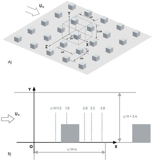
Figure 1.
(A) Schematic of the 3D computational domain for the flow past an array of cubes, (B) 2-D view of an XY plane with locations at which comparisons between numerical and experimental results were performed.
Two mesh sizes consisting of 55 × 45 × 55, and 150 × 180 × 150 nodes were used to discretize the computational domain. A total of three different meshes were utilized; the first had the lowest and nearly uniform grid density, i.e., 55 × 45 × 55, as shown in Figure 2a; the other two, as depicted in Figure 2b,c, were constructed with the larger mesh size, i.e., 150 × 180 × 150. The first had an almost uniform grid spacing throughout the domain, while the other had mesh refinements near the surface of the cube. The grid size and turbulence models used in the computations were carefully chosen after doing a thorough literature review on similar simulations. Table 1 shows details of the grid size used in this work and selected similar simulations from the literature. It is worth noting that for all three different grids used in this work, the Y+ and growth rate values, shown in Table 2, agree with the recommendations of the Young-Person’s guide to DES grids [49]. It is common practice to use relatively coarse grid sizes in the simulation of atmospheric boundary layers in the urban environment [10]. Therefore, the coarse mesh used herein will assess the ability of the model to accurately predict flow features on low-density grids. Nevertheless, using a denser mesh improves the model’s ability to resolve flow structures by reducing the effect of subgrid modeling. Moreover, the third mesh, that included grid-refinement interfaces both parallel and normal to the flow direction, served to assess the magnitude of the errors generated due to propagations of stresses across grid refinement interfaces.

Figure 2.
2D view of the three different meshes used in the simulations: (a) uniform coarse-mesh, (b) uniform fine mesh and (c) non-uniform clustered mesh.

Table 1.
Models and grid sizes for the simulation of flow past an array of cubes.

Table 2.
Values of y+, Δ+ and growth rate for all models and grids used for the flow past an array of cubes.
The flow initialization was done with a constant and uniform velocity, Ub, in the streamwise direction. However, in order to ensure that the initial conditions did not affect the obtained solution, the first 500 Tb of flow time were disregarded, and a total period of 200 Tb was averaged to ensure statistical convergence of flow variables. It is worth noting that Tb is the turnover time expressed as Tb = H/Ub, where H is the cube height, and the time step used in the calculations was set as ∆t = Tb/32. To prove that the solution is time-independent, the time step was further reduced to half of its original value for the simulation on the regular mesh using WMLES. The average velocities remained unchanged with the smaller time step, proving that the selection of the original time step was adequate. Figure 3 depicts the variation the streamwise velocity at vertical lines located in the XY plane (Z = 0) at various x-locations (Figure 1B) for all three tested turbulence models compared to the experimental data my Meinders et al. The plot was done on the three meshes discussed earlier; the unclustrered low- and high-density meshes are shown in Figure 3a, and a comparison between the clustered and unclustered meshes is shown in Figure 3b. All three turbulence models accurately predict the velocity variation when used on the unclustered high-density mesh. However, the One-Equation SAS model had the most accurate predictions of the coarse, low-density mesh. The advantage of using the One-Equation SAS model can be clearly inferred from Figure 3b; it is the only model that succeeds in reproducing the experimental velocity profiles on the clustered mesh with a 0.4% deviation from experimental data at x/H = 2.8, followed by the WMLES having a total error of 3.2%. Consequently, its superiority in generating accurate results on both uniform and non-uniform meshes is demonstrated. In Figure 4, the streamwise velocity profiles on horizontal lines (parallel to the z-axis) for the same meshes and models as in Figure 3, but on a plane parallel to the XZ plane at Y = 0.5 H, were plotted. The One-Equation SAS model predicts the most accurate results on the low-density mesh with a total deviation from experimental data of 1.62% at x/H = 2.8, followed by the IDDES, having an error of 3.6%, while the WMLES deviates by 6.53%. On the other hand, the WMLES model generates better predictions on the clustered mesh, with the highest deviations from experimental data at x/H = 3.8. On the other hand, the IDDES model performs poorly near the wall (0.0 < z/H < 0.6) on the clustered mesh and in the region where 1.0 < z/H < 2.0 on the unclustered uniform mesh. Figure 5 depicts the variation of the spanwise velocity on same plane and lines and for similar models and conditions as Figure 4. Of all the considered meshes, the IDDES and WMLES models produce the least accurate results. Additionally, predictions of the IDDES model on the clustered mesh show large deviations from the experimental data. On the other hand, the One-Equation SAS model shows the lowest deviation from experimental data on all three grids tested. Additionally, it is worth noting that the One-Equation SAS model succeeded in predicting the streamwise velocity with better accuracy (Figure 3 and Figure 4).

Figure 3.
Effect of (a) mesh density, and (b) mesh clustering on the average streamwise velocity in the XY plane cutting through the center of the cube at z/H = 0. Each successive x/H profile starting from the one at x/H =1.2 is offset by one unit from the previous profile.


Figure 4.
Effect of (a) mesh density, and (b) mesh clustering on the average streamwise velocity in the XZ plane cutting through the center of the cube at y/H = 0.5. Each successive x/H profile starting from the one at x/H = 1.2 is offset by one unit from the previous profile.
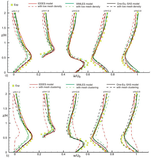
Figure 5.
Effect of (a) mesh density, and (b) mesh clustering on the average sapnwise velocity in the XZ plane cutting through the center of the cube at y/H = 0.5. Each successive x/H profile starting from the one at x/H = 1.2 is offset by one unit from the previous profile.
After assessing the models’ ability to predict streamwise and spanwise velocity profiles at various locations in the flow, plots of the normalized Reynolds stress, , were generated. The variation of streamwise Reynolds stress in the x-y plane with vertical location y/H, at various x-locations, is shown in Figure 6. The observed peaks in Reynolds stress at the rooftop of the cube (y = H) are due to the near-wall shear layers separating from the surface of the building. These peaks are well-predicted by all models on both the coarse and fine grids. However, the One-Equation SAS model mostly deviates from experimental data in the region extending between 2 consecutive cubes, above the rooftop of the cube (1.0 < y/H < 2.5). By examining Figure 6b, it is evident that the One-Equation SAS model is the most accurate at reproducing the Reynolds stress on the clustered mesh. Moreover, the IDDES model underpredicts the Reynolds stress in the near-wall region (0 < y/H < 1.0). Similarly, all models predict with reasonable accuracy the streamside Reynolds stress on a XZ plane at Y = 0.5 H for computations on both coarse and fine grids, as shown in Figure 7. Additionally, the IDDEs again underpredicts the stresses generated in the near-wall region.
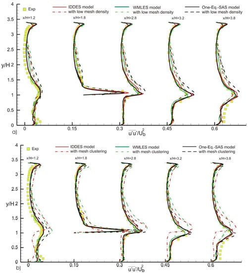
Figure 6.
Effect of (a) mesh density, and (b) mesh clustering on the streamwise normalized Reynolds stress in the XY plane cutting through the center of the cube at z/H = 0.
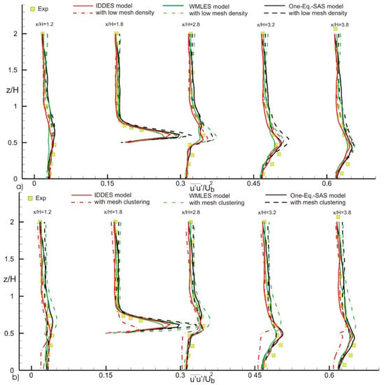
Figure 7.
Effect of (a) mesh density, and (b) mesh clustering on the streamwise normalized Reynolds stress in the XZ plane cutting through the center of the cube at y/H = 0.5.
When considering the spanwise normalized Reynolds normal stress, , on the XY plane described earlier and shown in Figure 1B, it can be concluded that the predictions generated by all models on both low- and high-density meshes are accurate for x/H = 1.8 and x/H = 2.8. However, large deviations are observed in the region where 0.0 < y/H < 1.0 for x/H = 1.2, 3.2 and 3.8 (see Figure 8a). The One-Equation SAS model performs slightly better in these regions of high deviations. The WMLES and IDDES models are not able to accurately model subgrid stress, and therefore, cannot accurately resolve Reynolds stress levels. When using grid refinement interfaces (Figure 8b), the deviations becomes more prominent for the WMLEs and IDDES models, while the One-Equation SAS model is relatively unaffected by the mesh clustering. These discrepancies were previously reported by Goodfriend et al. [10], and were attributed to the wave reflections that occur at grid refinement interfaces. Spanwise normalized Reynold stresses were also plotted on XZ plane at y = 0.5 H, as shown in Figure 9. In the near wall regions, both the WMLES and IDDES models predict low levels of Reynolds stress on the coarse mesh. Additionally, the effect of grid refinement shown in Figure 9b is detrimental for the IDDES and WMLES models, while its impact on the One-Equation SAS model is insignificant.
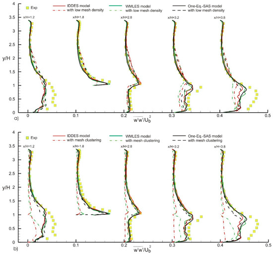
Figure 8.
Effect of (a) mesh density, and (b) mesh clustering on the spanwise normalized Reynolds stress in the XY plane cutting through the center of the cube at z/H = 0.

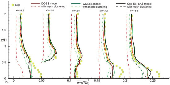
Figure 9.
Effect of (a) mesh density, and (b) mesh clustering on the spanwise normalized Reynolds stress in the XZ plane cutting through the center of the cube at y/H = 0.5.
The effect of grid density and clustering can be further explored by considering the Contours of spanwise normalized Reynolds normal stress, , on the x-y plane at the centerline of the cubes, as shown in Figure 10. A comparison of the concentration of , as predicted by the three models on the coarse grid, reveals discrepancies. Both the WMLES and the IDDES predict low levels of in circulatory regions upstream and downstream of the cube, as depicted in the first column of Figure 10. The One-Equation SAS model predicts the highest Reynolds normal stress concentration levels on the coarse grid in these regions, thereby exhibiting more accurate sub-grid modeling. All three models predict very similar distribution of on the regular mesh. This similarity in predicting the Reynolds normal stress levels is reflected by comparison of the solid lines in Figure 8. The last column of Figure 10 shows the effect of clustered mesh as predicted by the three models. Discontinuities in clustered regions, as predicted by the WMLES and IDDES models, are obvious, especially in the crossflow direction upstream and downstream of the cube. The One-Equation SAS model, however, does not show signs of discontinuity, as the model formulation is free of grid-scale.
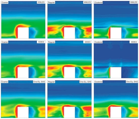
Figure 10.
Contours of normalized Reynolds stress in the XY plane cutting through the center of the cube at z/H = 0 for all three tested turbulence models on the uniform coarse and regular meshes and the non-uniform clustered mesh.
Flow Past a Circular Cylinder: This test case involves massive flow separation behind a circular cylinder. The objective here is to assess the extent to which the considered models are able to reproduce the flow features downstream the cylinder when subject to mesh refinements applied only in the wake region. A coarse mesh, consisting of 1.4762 × 10⁶ nodes, was used to assess the ability of the subgrid modeling. Two levels of grid adaptation were then applied adjacent to the cylinder in the wake region, resulting in a final mesh density of 4.8764 × 10⁶ nodes. Figure 11 depicts the original and the refined mesh. Grid adaptation was used to investigate the response of the models to local refinements, i.e., when resolving flow structures is of interest in local regions, which could arise in urban city layout. In the present case, refinements that encompass the cylinder, i.e., the separated shear layers, yielded similar results to those of the literature [52], and thus, are not included herein as they do not fall within the previously-set objectives.

Figure 11.
Mesh in the x-y plane that passes through the center of the cylinder, (a) coarse mesh, and (b) clustered mesh.
Numerical simulations are compared with the experimental measurements of Cantwell and Coles [53] at a Reynolds number of 140,000. The spanwise extension of the domain was 4 × D, which is considered acceptable for resolving turbulent flow structures. A periodic boundary condition was imposed in the spanwise direction, while the velocity inlet and pressure outlet boundary conditions were implemented at the inlet and the outlet of the domain. No unsteadiness was introduced at the inlet, as the global instabilities were sufficiently large to trigger unsteadiness in flow structures. Boundaries in the transverse direction were treated with symmetry conditions. A velocity magnitude of 2.045 m/s and a turbulent viscosity of 2 × 10⁻⁴ m2/s were set at the inlet. A zero-gauge pressure was set at the outlet boundary condition, while the turbulent viscosity value was extrapolated from the interior domain. A CFL of 0.7 was used with default relaxation and under-relaxation factors for all flow variables. For all models, the bounded central differencing scheme was selected as it involves acceptable numerical dissipation that is small enough not to affect the evolution of small-scale turbulent structures. A time step of 5 × 10⁻⁴ s was set for all models, which was several fold less than that of the experimental shedding period computed from the Strouhal number St of 0.179, and smaller by an order of magnitude when compared to simulations found in the literature using scale resolving models [52,54].
According to Cantwell and Coles [53], a small separation bubble formed behind the cylinder, the mean length of which was slightly more than half the diameter of the cylinder downstream the stagnation point. To assess the accuracy of the considered models in reproducing the separation bubble, their predicted centerline mean streamwise velocity profiles versus axial distance downstream of the cylinder were compared against experimental data in Figure 12. All three models fail to reproduce the extent of the separation bubble and the recovery velocity profile on the original coarse mesh. It is worth noting that a y+ < 0.092 was attained with all three models. It is clear that with this mesh coarseness, none of the models was able to predict subgrid scales. Similarly, Travin et al. [55] numerically assessed the impact of the grid size on the predictions of the roll-up shear vortices that occur right after boundary layer transition around a cylinder. Unfortunately, their grid sizes were not fine enough, leading to an under-resolved flow transition. The IDDES and the One-Equation SAS models slightly underpredict the extent of the recirculation bubble, while the WMLES model predicts an acceptable length of the separation bubble, albeit with a fast recovery that overpredicts the centerline mean velocity ratio. Refinement of the mesh in the wake region shows improvement in velocity profiles, as predicted by the IDDES and the One-Equation SAS models. The WMLES model shows no improvements; on the contrary, the model predicts a faster recovery. In both mesh scenarios, the WMLES model performs poorly in comparison to the other two models. This could be related to the simple nature of the model, which is based on a Smogarinsky, rendering it incapable of accounting for the near-wall turbulence at this mesh density. It is worth noting that the flow structure downstream of the cylinder is very much affected by its boundary layer development. Therefore, irrespective of the refinement in the wake region, the WMLES model fails to predict the wake velocity profile. On the contrary, the other two models performed better, as they rely on transport equation(s) to model turbulent mechanism.
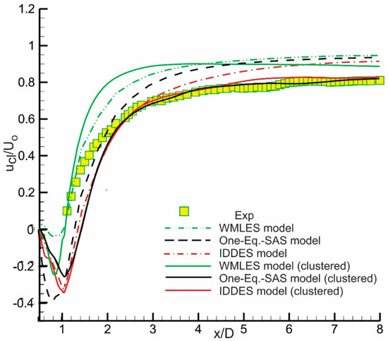
Figure 12.
Centerline mean streamwise velocity distribution showing the effect of coarse and clustered mesh on the predicted profile for the One-Equation SAS, WMLES, and IDDES models.
The profiles of normalized Reynolds normal stress in the horizontal (), and vertical (), directions at the centerline in the wake region are shown in Figure 13 and Figure 14, respectively. The One-Equation SAS model acceptably predicts the peak level of the streamwise Reynolds stress on the original coarse mesh. The IDDES model closely follows the One-Equation SAS model, while the WMLES returns very poor predictions. All models fail to predict the Reynolds normal stress distribution downstream of the recovery region x/d > 2. The results do not show major improvements with mesh refinements in the wake region. For the vertical normalized Reynolds normal stress distribution, the One-Equation SAS model returns the best predictions, followed by the IDDES and the WMLES models, respectively. Improvements here, due to mesh refinements, are more noticeable where all peaks shift towards the experimental one. The WMLES marks a substantial improvement on the refined mesh; however, it returns poor predictions compared to the other two models.
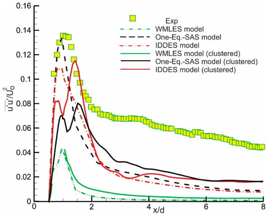
Figure 13.
Normalized Reynolds stress distribution on the centerline behind the cylinder in the wake region showing effect of mesh density for all three models.
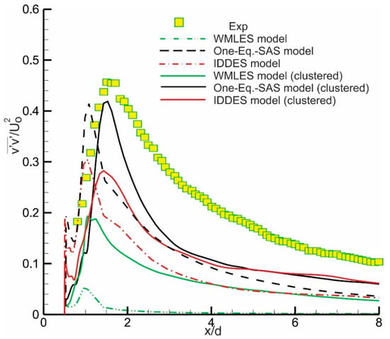
Figure 14.
Normalized Reynolds stress distribution on the centerline behind the cylinder in the wake region showing effect of mesh density for all three models.
A comparison of turbulent flow structures downstream of the cylinder using Q = 1.0 1/s2 colored by eddy viscosity ratio is shown in Figure 15. The effect of low mesh resolution on the resolved scales and viscosity ratio is clearly visible in the upper part of Figure 15. By comparing the turbulent flow structures of the considered models, it becomes evident that with a decrease in mesh resolution, small scales disappear and large scales emerge, accompanied by higher levels of eddy turbulent viscosity ratios. Mesh-refined flow scales are depicted in the bottom part of Figure 15. Despite the mesh refinement, the WMLES does not seem to be able to resolve as many scales as the IDDES and the One-Equation SAS models; this could be due to the near-wall eddy viscosity modeling that was mentioned earlier. As expected, all models dissipate lower levels of eddy viscosity behind the cylinder with smaller scales on the refined mesh. It is important to note that while the eddy viscosity is proportional to the grid scale in both of the IDDES and WMLES models, the One-Equation SAS model adjusts the eddy viscosity levels based on the Von Karman length scale, and subsequently, the flow structures in the wake region.
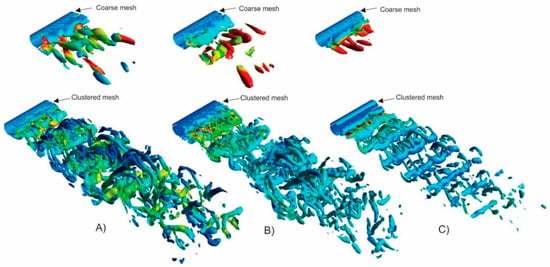
Figure 15.
Effect of low mesh resolution on turbulent flow structures. Iso-surface of Q = S2 − Ω2 = 1, colored by eddy viscosity ratio. (A) One-Equation SAS model, (B) IDDES model, (C) WMLES model.
5. Conclusions
Three turbulence models that belong to the closure family, i.e., algebraic, one-equation and two-equation models, were examined over two globally unstable test cases that involved massive flow separation. Unlike the WMLES and the IDDES, which depend on the grid scale, the proposed One-Equation SAS model relies on the Von-Kármán length scale.
Simulations of the flow over an array of cubic, urban-like obstacles were performed on coarse, fine and clustered meshes. The results showed that the One-Equation SAS model accurately predicts flow structures, regardless of the grid size. Additionally, the performance of the One-Equation SAS model on the clustered grids was superior to both IDDES and WMLES. However, the performance of all these models might vary with an increase in Re/Reτ. The most accurate predictions of the velocity and normalized and Reynolds stress profiles on coarse or non-uniform clustered grids were achieved by the One-Equation SAS model, followed by the WMLES model. It is worth noting that the IDDES model required the lowest number of iterations per time-step to reach convergence. This could be attributed to the elevated levels of dissipation compared to the other two models, a point that merits further investigation in future work.
For the circular cylinder test case, grid refinement in the wake region did not improve the performance of the WMLES model. However, improvements were noticed in the velocity profiles downstream of the separation bubble, as predicted by the One-Equation SAS and IDDES models. Similar behavior was noticed with normalized Reynolds stress profiles, where only the One-Equation SAS and IDDES models performed better on the refined mesh. These models can be better used on coarse meshes, and both seem to be less susceptible to mesh resolution and uninformed refinements.
While it was possible to use WMLES to model bluff bodies such as the array of cubes, flows that are boundary layer-dependent (i.e., they evolve based on the separated shear layer) cannot be modeled by a simple Smogarinsky-like model, irrespective of the utilized time step. The IDDES was able to model the circular cylinder test case; however, it poorly performed on the array of cubes test case when run on coarse and clustered meshes, and returned acceptable performance on the regular mesh. In general, the One-Equation SAS model, which does not depend on the mesh scale, had the best performance for both test cases.
Author Contributions
Conceptualization, M.E.; methodology, M.E.; software, M.E.; validation, A.E., and M.E.; formal analysis, A.E.; investigation, A.E.; resources, M.E.; data curation, M.E. and A.E.; writing—original draft preparation, M.E. and A.E.; writing—review and editing, M.E. and A.E.; visualization, M.E. and A.E.; supervision, M.E.; project administration, M.E.; funding acquisition, M.E.
Funding
This research received no external funding.
Conflicts of Interest
The authors declare no conflicts of interest.
References
- Tominaga, Y.; Stathopoulos, T. CFD Modeling of Pollution Dispersion in Building Array: Evaluation of turbulent scalar flux modeling in RANS model using LES results. J. Wind Eng. Ind. Aerodyn. 2012, 104–106, 484–491. [Google Scholar] [CrossRef]
- Wright, N.G.; Easom, G.J. Non-linear k-ε turbulence model results for flow over a building at full-scale. Appl. Math. Model. 2003, 27, 1013–1033. [Google Scholar] [CrossRef]
- Kubilay, A.; Neophytou, M.K.A.; Matsentides, S.; Loizou, M.; Carmeliet, J. The pollutant removal capacity of urban street canyons as quantified by the pollutant exchange velocity. Urban Clim. 2017, 21, 136–153. [Google Scholar] [CrossRef]
- Nazarian, N.; Kleissl, J. CFD simulation of an idealized urban environment: Thermal effects of geometrical characteristics and surface materials. Urban Clim. 2015, 12, 141–159. [Google Scholar] [CrossRef]
- Hu, Z.X.; Cui, G.X.; Zhang, Z.S. Numerical study of mixed convective heat transfer coefficients for building cluster. J. Wind Eng. Ind. Aerodyn. 2018, 172, 170–180. [Google Scholar] [CrossRef]
- Coceal, O.; Thomas, T.G.; Castro, I.P.; Belcher, S.E. Mean flow and turbulence statistics over groups of urban-like cubical obstacles. Bound.-Layer Meteorol. 2006, 121, 491–519. [Google Scholar] [CrossRef]
- Xie, Z.; Castro, I.P. LES and RANS for turbulent flow over arrays of wall-mounted obstacles. Flow Turbul. Combust. 2006, 76, 291–312. [Google Scholar] [CrossRef]
- Basara, B. Fluid flow and conjugate heat transfer in a matrix of surface-mounted cubes: A PANS study. Int. J. Heat Fluid Flow 2015, 51, 166–174. [Google Scholar] [CrossRef]
- Cheng, Y.; Lien, F.S.; Yee, E.; Sinclair, R. A comparison of large Eddy simulations with a standard k-ε Reynolds-averaged Navier-Stokes model for the prediction of a fully developed turbulent flow over a matrix of cubes. J. Wind Eng. Ind. Aerodyn. 2003, 91, 1301–1328. [Google Scholar] [CrossRef]
- Goodfriend, E.; Chow, F.K.; Vanella, M.; Balaras, E. Large-Eddy Simulation of Flow Through an Array of Cubes with Local Grid Refinement. Bound.-Layer Meteorol. 2016, 159, 285–303. [Google Scholar] [CrossRef]
- Razak, A.A.; Hagishima, A.; Ikegaya, N.; Tanimoto, J. Analysis of airflow over building arrays for assessment of urban wind environment. Build. Environ. 2013, 59, 56–65. [Google Scholar] [CrossRef]
- Moonen, P.; Dorer, V.; Carmeliet, J. Effect of flow unsteadiness on the mean wind flow pattern in an idealized urban environment. J. Wind Eng. Ind. Aerodyn. 2012, 104–106, 389–396. [Google Scholar] [CrossRef]
- Gousseau, P.; Blocken, B.; Stathopoulos, T.; van Heijst, G.J.F. CFD simulation of near-field pollutant dispersion on a high-resolution grid: A case study by LES and RANS for a building group in downtown Montreal. Atmos. Environ. 2011, 45, 428–438. [Google Scholar] [CrossRef]
- Calhoun, R.; Gouveia, F.; Shinn, J.; Chan, S.; Stevens, D.; Lee, R.; Leone, J. Flow around a Complex Building: Experimental and Large-Eddy Simulation Comparisons. J. Appl. Meteorol. 2005, 44, 571–590. [Google Scholar] [CrossRef]
- Ricciardelli, F.; Polimeno, S. Some characteristics of the wind flow in the lower Urban Boundary Layer. J. Wind Eng. Ind. Aerodyn. 2006, 94, 815–832. [Google Scholar] [CrossRef]
- Lateb, M.; Meroney, R.N.; Yataghene, M.; Fellouah, H.; Saleh, F.; Boufadel, M.C. On the use of numerical modelling for near-field pollutant dispersion in urban environments—A review. Environ. Pollut. 2016, 208, 271–283. [Google Scholar] [CrossRef]
- Stathopoulos, T. Computational wind engineering: Past achievements and future challenges. J. Wind Eng. Ind. Aerodyn. 1997, 67–68, 509–532. [Google Scholar] [CrossRef]
- Santiago, A.D.J.L.; Martin, A.M.F.; Pinelli, A. Comparison Between Large-Eddy Simulation and Reynolds-Averaged Navier—Stokes Computations for the MUST Field Experiment. Part II: Effects of Incident Wind Angle Deviation on the Mean Flow and Plume Dispersion. Bound.-Layer Meteorol. 2010, 135, 133–150. [Google Scholar] [CrossRef]
- Mohamed, S.; Buccolieri, R.; Chan, A.; Di, S. Numerical simulation of atmospheric pollutant dispersion in an urban street canyon: Comparison between RANS and LES. J. Wind Eng. Ind. Aerodyn. 2011, 99, 103–113. [Google Scholar] [CrossRef]
- Tominaga, Y.; Stathopoulos, T. CFD modeling of pollution dispersion in a street canyon: Comparison between LES and RANS. J. Wind Eng. Ind. Aerodyn. 2011, 99, 340–348. [Google Scholar] [CrossRef]
- Xie, Z.; Castro, I.P. Large-eddy simulation for flow and dispersion in urban streets. Atmos. Environ. 2009, 43, 2174–2185. [Google Scholar] [CrossRef]
- Tominaga, Y.; Stathopoulos, T. Numerical simulation of dispersion around an isolated cubic building: Comparison of various types of k–ε models. Atmos. Environ. 2009, 43, 3200–3210. [Google Scholar] [CrossRef]
- Tominaga, Y.; Stathopoulos, T. CFD simulation of near-field pollutant dispersion in the urban environment: A review of current modeling techniques. Atmos. Environ. 2013, 79, 716–730. [Google Scholar] [CrossRef]
- Longo, R.; Ferrarotti, M.; Sánchez, C.G.; Derudi, M.; Parente, A. Advanced turbulence models and boundary conditions for flows around different configurations of ground-mounted buildings. J. Wind Eng. Ind. Aerodyn. 2017, 167, 160–182. [Google Scholar] [CrossRef]
- Piomelli, B.U.; Kang, S.; Ham, F.; Iaccarino, G. Effect of Discontinuous Filter Width in Large-Eddy Simulations of Plane Channel Flow. In Center for Turbulence Research Proceedings of the Summer Program 2006, Stanford University, CA, USA, 9 July–4 August 2006. [Google Scholar]
- Vanella, M.; Piomelli, U.; Balaras, E. Effect of grid discontinuities on large-eddy simulation statistics and flow fields. J. Turbul. 2008, 9, 5248. [Google Scholar] [CrossRef]
- Elkhoury, M.; Elcheik, A. Scale-resolving simulation of flow through a periodic array of cubes. WIT Trans. Eng. Sci. 2018, 120, 161–172. [Google Scholar] [CrossRef]
- Menter, F.; Kuntz, M.; Bender, R. A Scale-Adaptive Simulation Model for Turbulent Flow Predictions. In Proceedings of the 41st Aerospace Sciences Meeting Exhibit, Reno, NV, USA, 6–9 January 2003; American Institute of Aeronautics and Astronautics: Reston, VA, USA, 2003. [Google Scholar] [CrossRef]
- Menter, F.R. Eddy Viscosity Transport Equations and Their Relation to the k-ε Model. J. Fluids Eng. 1997, 119, 876–884. [Google Scholar] [CrossRef]
- Elkhoury, M. Assessment and Modification of One-Equation Models of Turbulence for Wall-Bounded Flows. J. Fluids Eng. 2007, 129, 921–928. [Google Scholar] [CrossRef]
- Elkhoury, M. Modified Menter Model in Comparison with Recently Developed Single-Equation Turbulence Closures. AIAA J. 2011, 49, 1399–1408. [Google Scholar] [CrossRef]
- Elkhoury, M. A low-Reynolds-number one-equation model of turbulence. Aeronaut. J. 2008, 112, 101–108. [Google Scholar] [CrossRef]
- Shur, M.L.; Spalart, P.R.; Strelets, M.K.; Travin, A.K. A hybrid RANS-LES approach with delayed-DES and wall-modelled LES capabilities. Int. J. Heat Fluid Flow 2008, 29, 1638–1649. [Google Scholar] [CrossRef]
- Menter, F.; Egorov, Y. A Scale Adaptive Simulation Model using Two-Equation Models. In Proceedings of the 43rd AIAA Aerospace Sciences Meeting Exhibit, Reno, NV, USA, 10–13 January 2005; American Institute of Aeronautics and Astronautics: Reston, VA, USA, 2005. [Google Scholar] [CrossRef]
- Elkhoury, M. Partially Lagging One-Equation Turbulence Model. AIAA J. 2015, 53, 3661–3673. [Google Scholar] [CrossRef]
- Albring, W. J. C. Rotta, Turbulente Strömungen. (Leitfäden der angewandten Mathematik und Mechanik, Band 15). 267 S. m. 104 Fig. Stuttgart 1972. B. G. Teubner. Preis geb. 68,—DM. ZAMM J. Appl. Math. Mech. Z. Angew. Math. Mech. 1974, 54, 129–130. [Google Scholar] [CrossRef]
- ANSYS® Academic Research Mechanical. Release 18.1. Canonsburg, PA 15317, USA.
- Chorin, A.J. Numerical Solution of the Navier-Stokes Equations. Math. Comput. 1968, 22, 745. [Google Scholar] [CrossRef]
- Dejoan, A.; Leschziner, M.A. Large eddy simulation of a plane turbulent wall jet. Phys. Fluids 2005, 17, 025102. [Google Scholar] [CrossRef]
- Akselvoll, K.; Moin, P. Large-eddy simulation of turbulent confined coannular jets. J. Fluid Mech. 1996, 315, 387–411. [Google Scholar] [CrossRef]
- Eggels, J.G.M.; Unger, F.; Weiss, M.H.; Westerweel, J.; Adrian, R.; Friedrich, R.; Nieuwstadt, F.T.M. Fully Developed Turbulent Pipe Flow: A Comparison Between Direct Numerical Simulation and Experiment. J. Fluid Mech. 1994, 268, 175–210. [Google Scholar] [CrossRef]
- Choi, H.; Moin, P.; Kim, J. Turbulent Drag Reduction: Studies of Feedback Control and Flow over Riblets; Tech. Rep. Report TF-55; Stanford, CA, USA, 1992. [Google Scholar]
- Boersma, B.J.A.; Brethouwer, G.A.; Nieuwstadt, F.T.M.A. A numerical investigation on the effect of the inflow conditions on the self-similar region of a round jet. Phys. Fluids 1998, 10, 899–909. [Google Scholar] [CrossRef]
- Pierce, C.D.; Moin, P. Progress-variable approach for large-eddy simulation of non-premixed turbulent combustion. J. Fluid Mech. 2004, 504, 73–97. [Google Scholar] [CrossRef]
- Kim, J.; Choi, H. Large eddy simulation of a circular jet: Effect of inflow conditions on the near field. J. Fluid Mech. 2009, 620, 383–411. [Google Scholar] [CrossRef]
- Elkhoury, M. Assessment of turbulence models for the simulation of turbulent flows past bluff bodies. J. Wind Eng. Ind. Aerodyn. 2016, 154, 10–20. [Google Scholar] [CrossRef]
- Meinders, E.R. Experimental Study of Heat Transfer in Turbulent Flows over Wall-Mounted Cubes; Delft University of Technology: Delft, The Netherlands, 1998. [Google Scholar]
- Meinders, E.R.; Hanjalić, K. Vortex structure and heat transfer in turbulent flow over a wall-mounted matrix of cubes. Int. J. Heat Fluid Flow 1999, 20, 255–267. [Google Scholar] [CrossRef]
- Spalart, R. Young-Person’s Guide Simulation Grids Detached-Eddy; NASA: Hampton, VA, USA, 2001.
- Hsieh, K.-J.; Lien, F.-S.; Yee, E. Towards a Unified Turbulence Simulation Approach for Wall-Bounded Flows. Flow Turbul. Combust. 2010, 84, 193. [Google Scholar] [CrossRef]
- Yang, X.I.A.; Sadique, J.; Mittal, R.; Meneveau, C. Integral wall model for large eddy simulations of wall-bounded turbulent flows. Phys. Fluids 2015, 27, 25112. [Google Scholar] [CrossRef]
- Zheng, W.; Yan, C.; Liu, H.; Luo, D. Comparative assessment of SAS and DES turbulence modeling for massively separated flows. Acta Mech. Sin. 2016, 32, 12–21. [Google Scholar] [CrossRef]
- Cantwell, B.; Coles, D. An experimental study of entrainment and transport in the turbulent near wake of a circular cylinder. J. Fluid Mech. 1983, 136, 321. [Google Scholar] [CrossRef]
- Catalano, P. Numerical simulation of the flow around a circular cylinder at high Reynolds numbers. Int. J. Heat Fluid Flow 2003, 24, 463–469. [Google Scholar] [CrossRef]
- Travin, A.; Shur, M.; Strelets, M.; Spalart, P. Detached-eddy simulations past a circular cylinder. Flow Turbul. Combust. 2000, 63, 293–313. [Google Scholar] [CrossRef]
© 2019 by the authors. Licensee MDPI, Basel, Switzerland. This article is an open access article distributed under the terms and conditions of the Creative Commons Attribution (CC BY) license (http://creativecommons.org/licenses/by/4.0/).