A Multi-Scale Modeling Approach for Simulating Crack Sensing in Polymer Fibrous Composites Using Electrically Conductive Carbon Nanotube Networks. Part II: Meso- and Macro-Scale Analyses


Abstract
:
1. Introduction
2. Meso-Scale Model
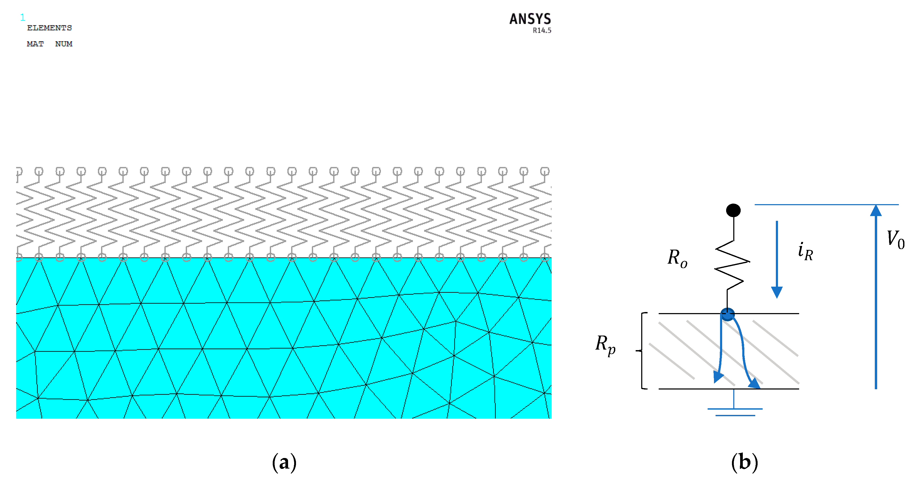
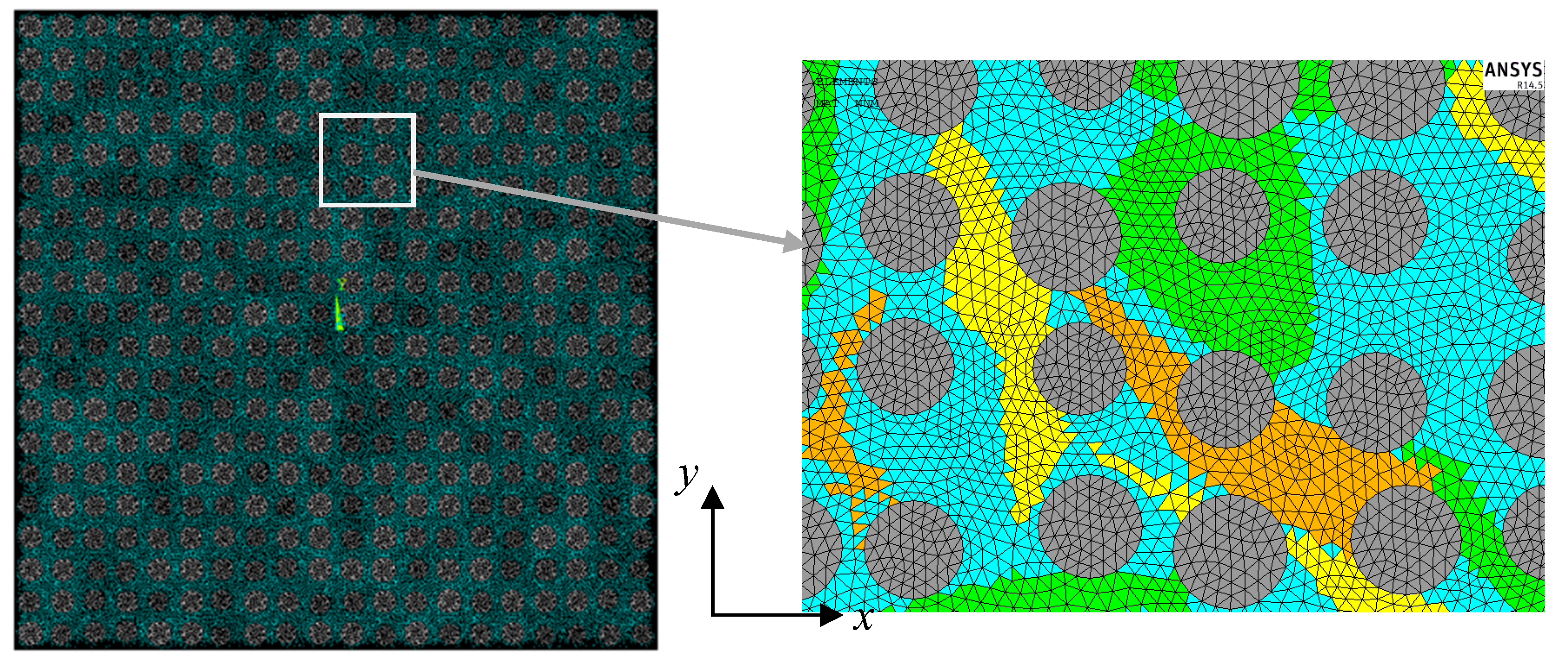
2.1. Geometry and FE Model
2.2. Imposed Electric Field
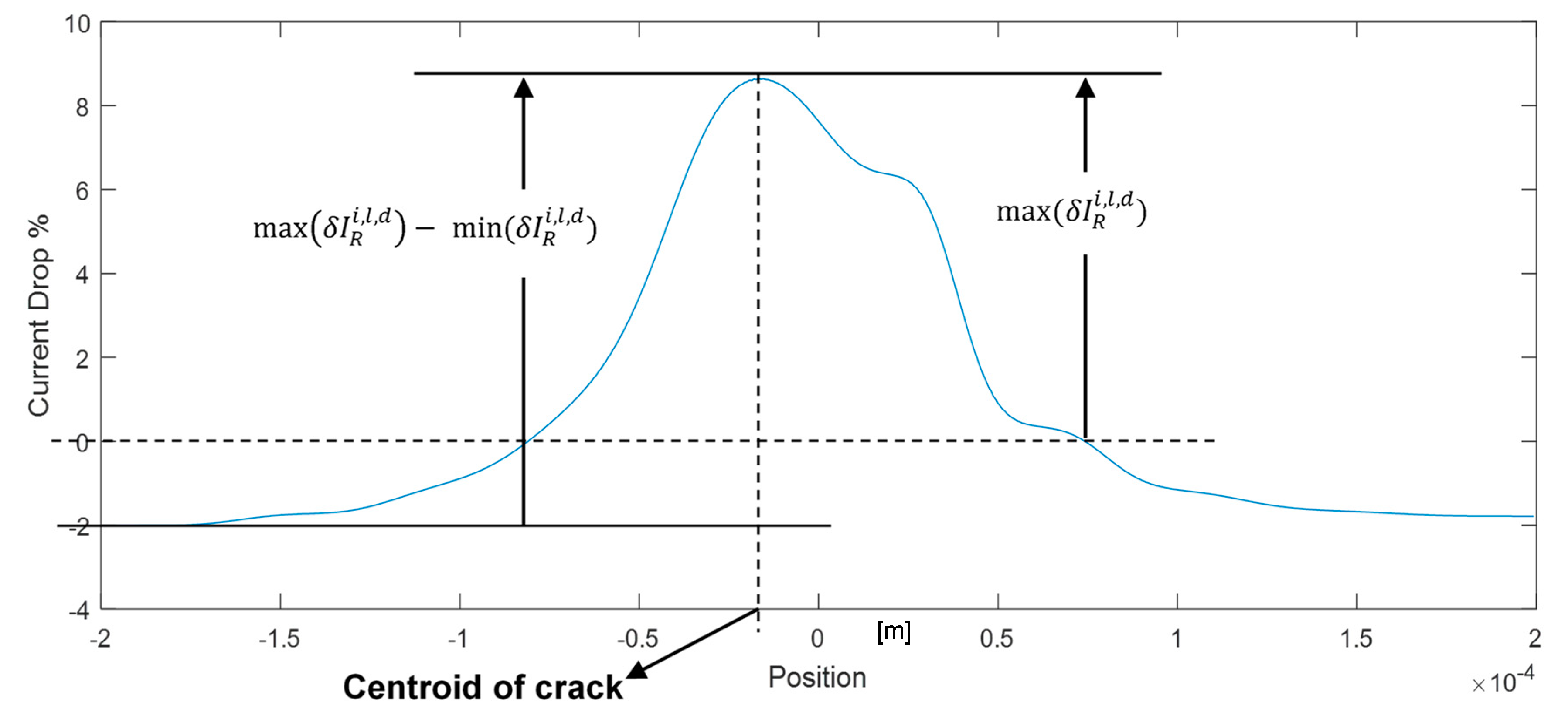
2.3. Crack Sensing Methodology
3. Macro-Scale Model
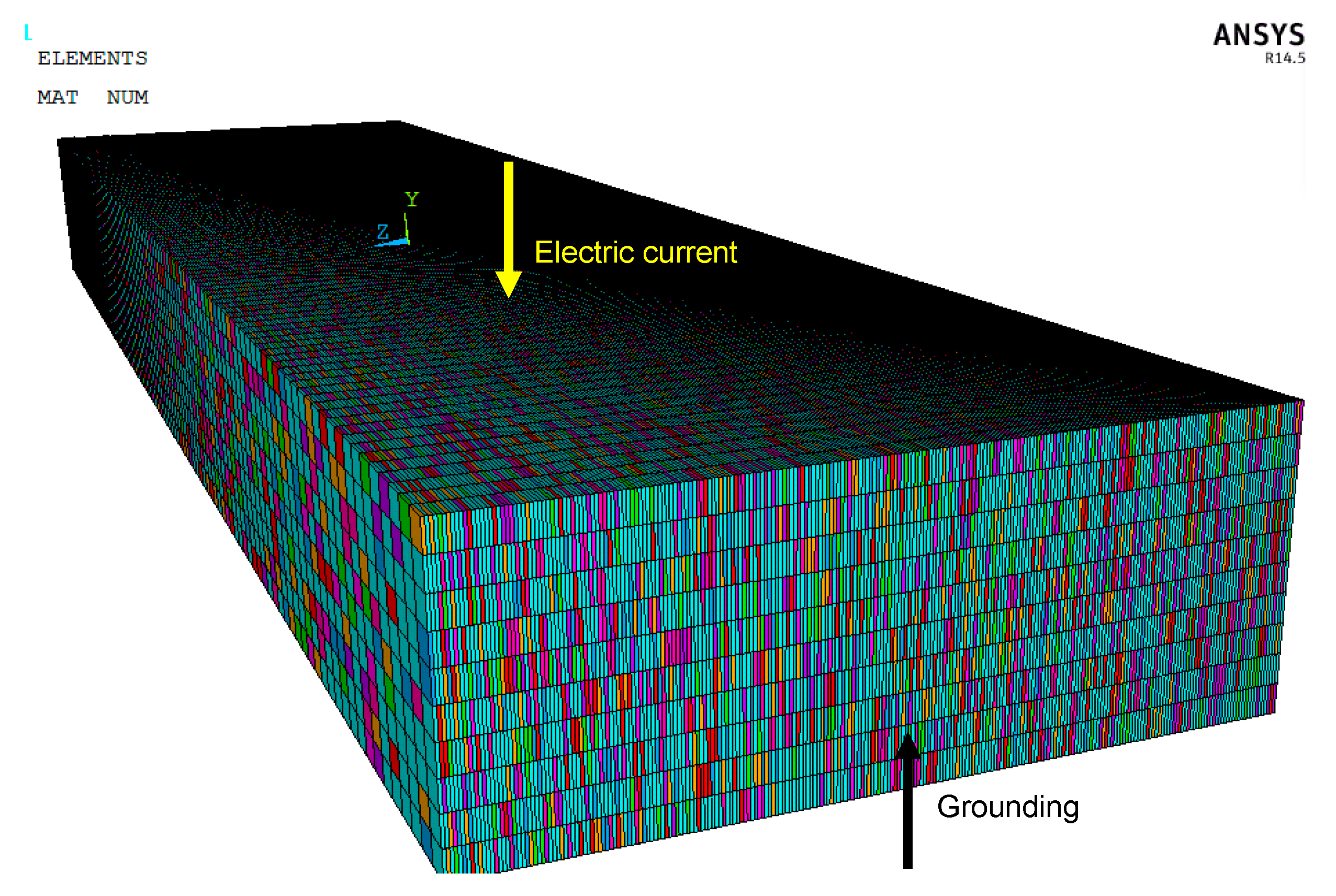
3.1. Geometry and FE Modeling
3.2. Introduction of a Virtual Crack, Charging and Computations
4. Numerical Results
4.1. Meso-Scale: Effect of Crack Presence
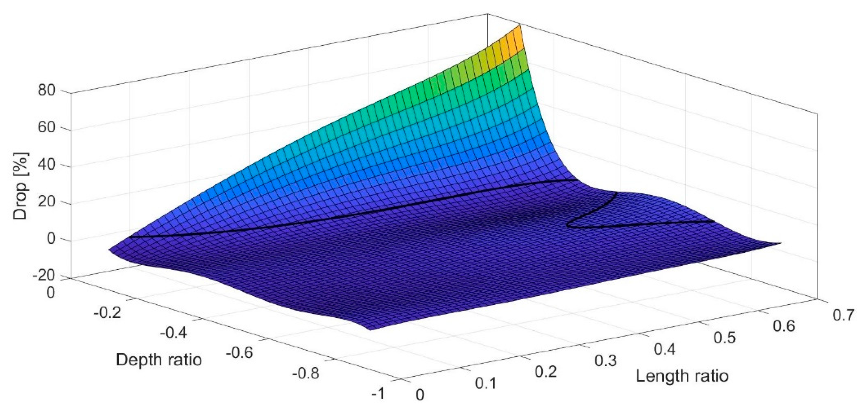
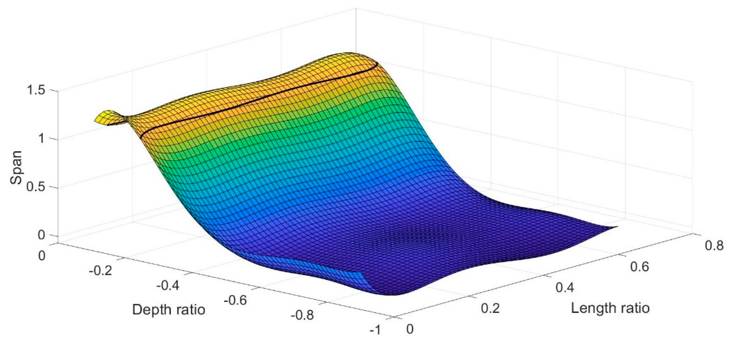
4.2. Macro-Scale: Crack Detection
5. Conclusions
Author Contributions
Funding
Conflicts of Interest
References
- Boller, C. Why SHM? A Motivation. In NATO Lecture Series STO-MP-AVT-220 Structural Health Monitoring of Military Vehicles: STO Educational Notes; NATO STO: Brussels, Belgium, 2014. [Google Scholar]
- Duong, H.M.; Gong, F.; Liu, P.; Tran, T.Q. Advanced Fabrication and Properties of Aligned Carbon Nanotube Composites: Experiments and Modeling. Available online: https://www.intechopen.com/books/carbon-nanotubes-current-progress-of-their-polymer-composites/advanced-fabrication-and-properties-of-aligned-carbon-nanotube-composites-experiments-and-modeling (accessed on 5 October 2017).
- Tran, T.Q.; Headrick, R.J.; Bengio, E.A.; Myo Myint, S.; Khoshnevis, H.; Jamali, V.; Duong, H.M.; Pasquali, M. Purification and Dissolution of Carbon Nanotube Fibers Spun from the Floating Catalyst Method. Appl. Mater. Interfaces 2017, 9, 37112–37119. [Google Scholar] [CrossRef] [PubMed]
- Tserpes, K.I.; Papanikos, P. Finite element modeling of single-walled carbon nanotubes. Compos. Part B 2005, 36, 468–477. [Google Scholar] [CrossRef]
- Papanikos, P.; Nikolopoulos, D.D.; Tserpes, K.I. Equivalent beams for carbon nanotubes. Comput. Mater. Sci. 2008, 43, 345–352. [Google Scholar] [CrossRef]
- Tserpes, K.I.; Papanikos, P.; Tsirkas, S.A. A progressive fracture model for carbon nanotubes. Compos. Part. B 2006, 37, 662–669. [Google Scholar] [CrossRef]
- Tserpes, K.I.; Papanikos, P. The effect of Stone-Wales defect on the tensile behavior and fracture of single-walled carbon nanotubes. Compos. Struct. 2007, 79, 581–589. [Google Scholar] [CrossRef]
- Kim, P.; Shi, L.; Majumdar, A.; Mc Euen, P.L. Thermal transport measurements of individual multiwalled nanotube. Phys. Rev. Lett. 2001, 87, 215502. [Google Scholar] [CrossRef] [PubMed]
- Ebbesen, T.W.; Lezec, H.J.; Hiura, H.; Bennett, J.W.; Ghaemi, H.F.; Thio, T. Electrical conductivity of individual carbon nanotubes. Nature 1996, 382, 54–56. [Google Scholar] [CrossRef]
- Fiedler, B.; Gojny, F.H.; Wichmann, M.H.G.; Bauhofer, W.; Karl, S. Can carbon nanotubes be used to sense damage in composites? Eur. J. Control. 2004, 29, 81–94. [Google Scholar] [CrossRef]
- Gallo, G.J.; Thostenson, E.T. Electrical characterization and modeling of carbon nanotube and carbon fiber self-sensing composites for enhanced sensing of microcracks. Mater. Today Commun. 2015, 3, 17–26. [Google Scholar] [CrossRef]
- Aly, Κ.; Li, A.; Bradford, P.D. Strain sensing in composites using aligned carbon nanotube sheets embedded in the interlaminar region. Compos. Part. A 2016, 90, 536–548. [Google Scholar] [CrossRef]
- Li, C.; Chou, T.W. Modeling of damage sensing in fiber composites using carbon nanotube networks. Compos. Sci. Technol. 2008, 68, 3373–3379. [Google Scholar] [CrossRef]
- Kuronuma, Y.; Takeda, T.; Shindo, Y.; Narita, F.; Wei, Z. Electrical resistance-based strain sensing in carbon nanotube/polymer composites under tension: Analytical modeling and experiments. Compos. Sci. Technol. 2012, 72, 1678–1682. [Google Scholar] [CrossRef]
- Tserpes, K.; Kora, Ch. A multi-scale modeling approach for simulating crack sensing in polymer fibrous composites using electrically conductive carbon nanotube networks. Part II: Micro-scale analysis. Comput. Mater. Sci. 2018, 154, 530–537. [Google Scholar] [CrossRef]
- ANSYS User’s Manual, version 11; Swanson Analysis Systems: Pittsburgh, PA, USA, 2008.


| Parameter/Property | Value |
|---|---|
| Fiber’s diameter | 6–8 μm |
| Fiber volume fraction | 55% |
| Fiber’s electrical conductivity at Υ direction, | 104 S/m |
| Fiber’s electrical conductivity at X direction, | 104 S/m |
| Electrical conductivity of polymeric matrix variation, | [3.77 × 10⁻⁵, 1.12 × 10⁻³, 3.28 × 10⁻³, 5.06 × 10⁻³, 8.77 × 10⁻³] S/m |
| Electrical resistance of circuit elements | 103 Ohm |
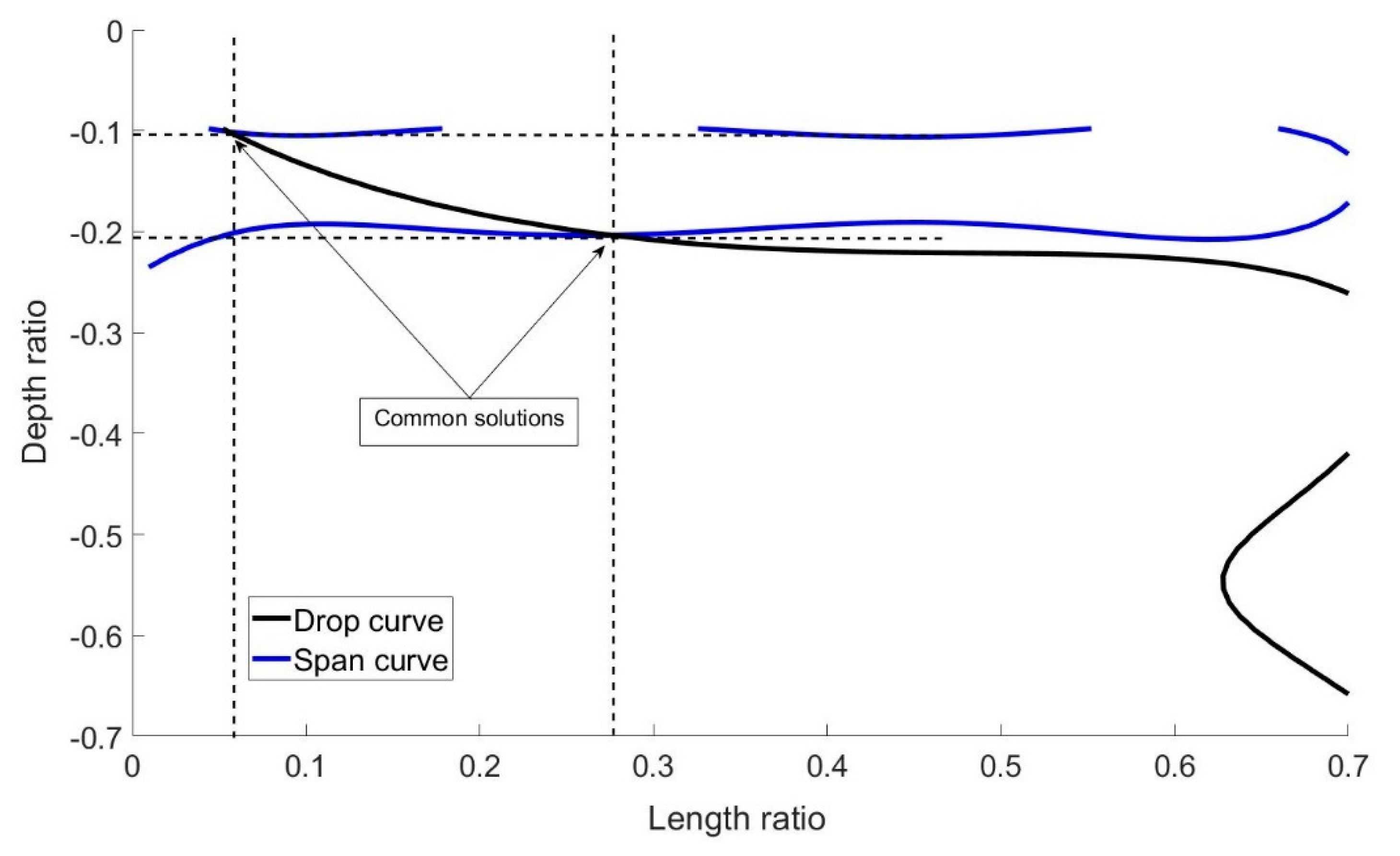
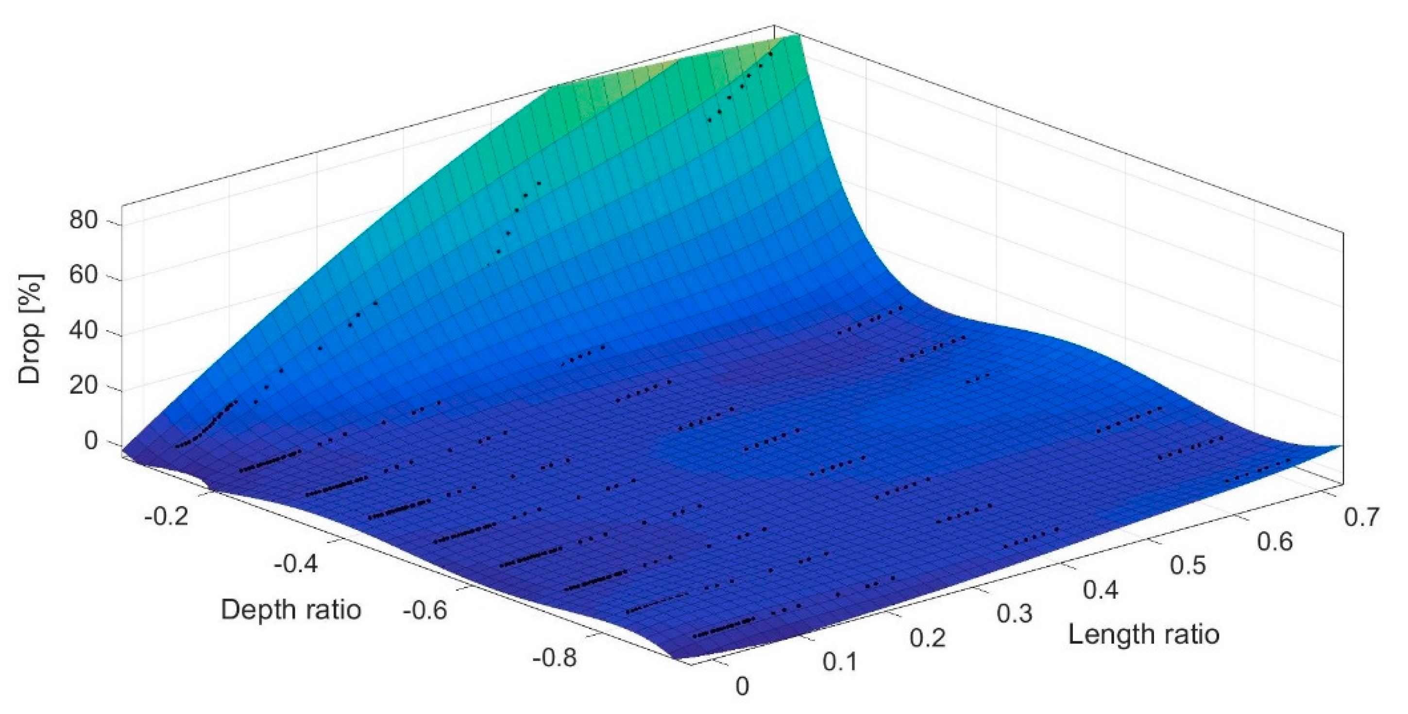
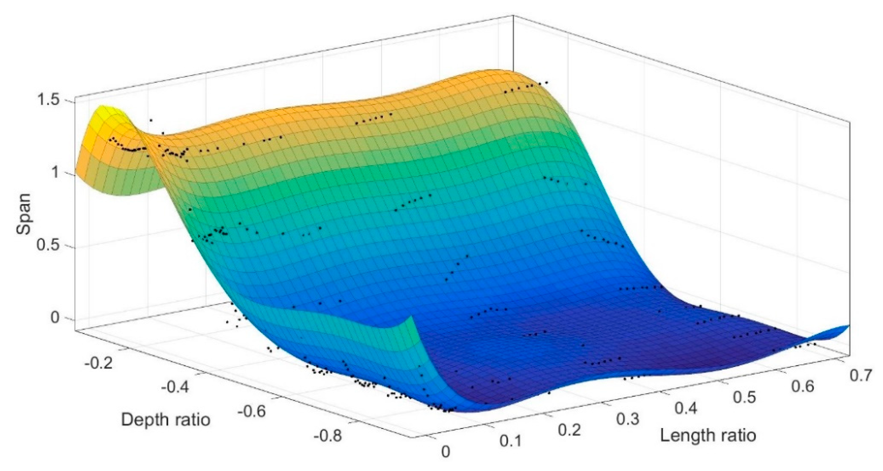
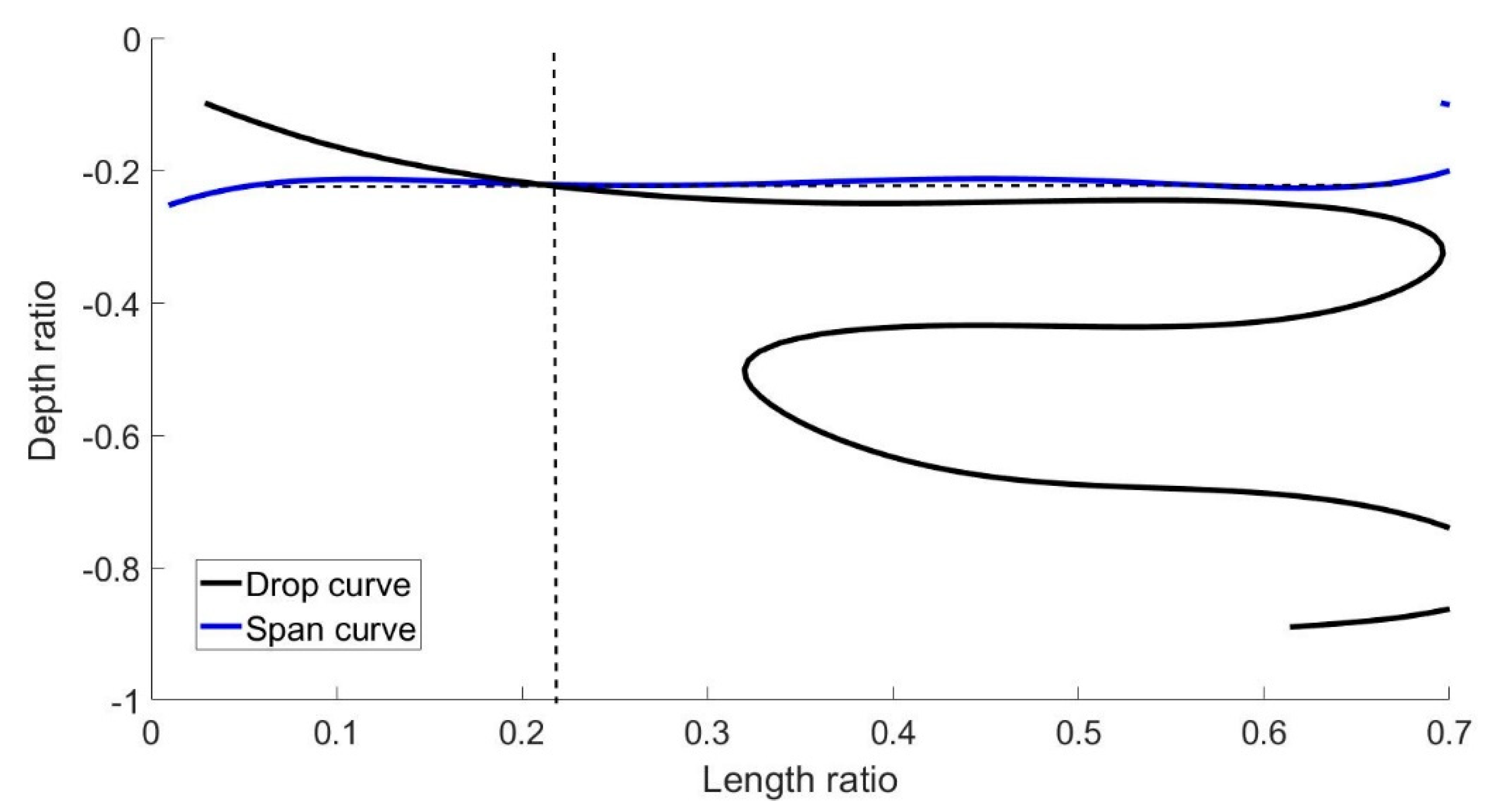
| Length Ratio, | Drop (%) | Span |
|---|---|---|
| 0.009 | 0.376 | 1.256 |
| 0.015 | 0.426 | 1.262 |
| 0.019 | 0.629 | 1.238 |
| 0.023 | 0.763 | 1.214 |
| 0.029 | 1.328 | 1.203 |
| 0.031 | 1.724 | 1.177 |
| 0.036 | 2.178 | 1.170 |
| 0.040 | 3.343 | 1.164 |
| 0.043 | 3.832 | 1.157 |
| 0.047 | 4.508 | 1.151 |
| 0.050 | 5.250 | 1.152 |
| 0.052 | 6.457 | 1.152 |
| 0.057 | 7.012 | 1.153 |
| 0.060 | 7.850 | 1.153 |
| 0.066 | 8.794 | 1.153 |
| 0.067 | 9.345 | 1.152 |
| 0.070 | 9.897 | 1.145 |
| 0.072 | 10.15 | 1.149 |
| 0.077 | 10.64 | 1.148 |
| 0.100 | 8.644 | 1.232 |
| 0.112 | 12.920 | 1.208 |
| 0.129 | 17.400 | 1.193 |
| 0.174 | 21.664 | 1.181 |
| 0.208 | 27.084 | 1.170 |
| 0.218 | 29.910 | 1.166 |
| 0.237 | 32.345 | 1.162 |
| 0.367 | 35.678 | 1.159 |
| 0.379 | 38.693 | 1.157 |
| 0.390 | 44.412 | 1.155 |
| 0.400 | 51.903 | 1.151 |
| 0.410 | 56.378 | 1.149 |
| 0.426 | 59.376 | 1.147 |
| 0.622 | 65.263 | 1.144 |
| 0.633 | 67.230 | 1.142 |
| 0.645 | 71.411 | 1.141 |
| 0.660 | 74.113 | 1.141 |
| 0.667 | 77.364 | 1.142 |
| 0.681 | 79.746 | 1.143 |
| 0.692 | 83.053 | 1.146 |
| Parameter/Property | Value |
|---|---|
| Theoritical fiber volume fraction | 55% |
| Transverse electrical conductivity variation | [1.13 × 10⁻⁴, 3.47 × 10⁻³, 4.02 × 10⁻³, 5.77 × 10⁻³, 9.32 × 10⁻³] S/m |
| Fiber’s electrical conductivity at Z direction, | 105 S/m |
| Electrical resistance of circuit elements | 103 Ohm |
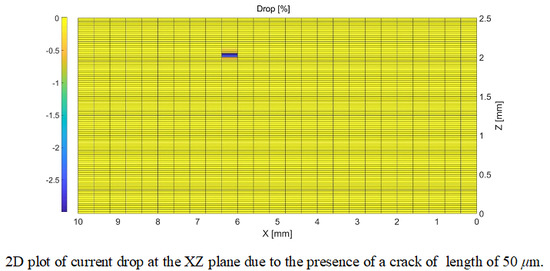
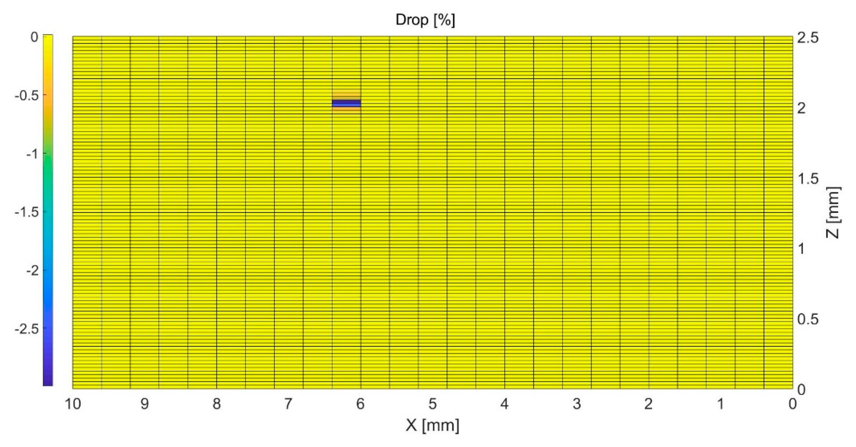
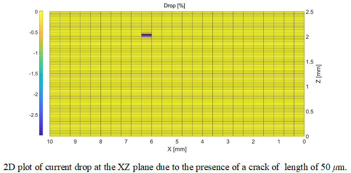
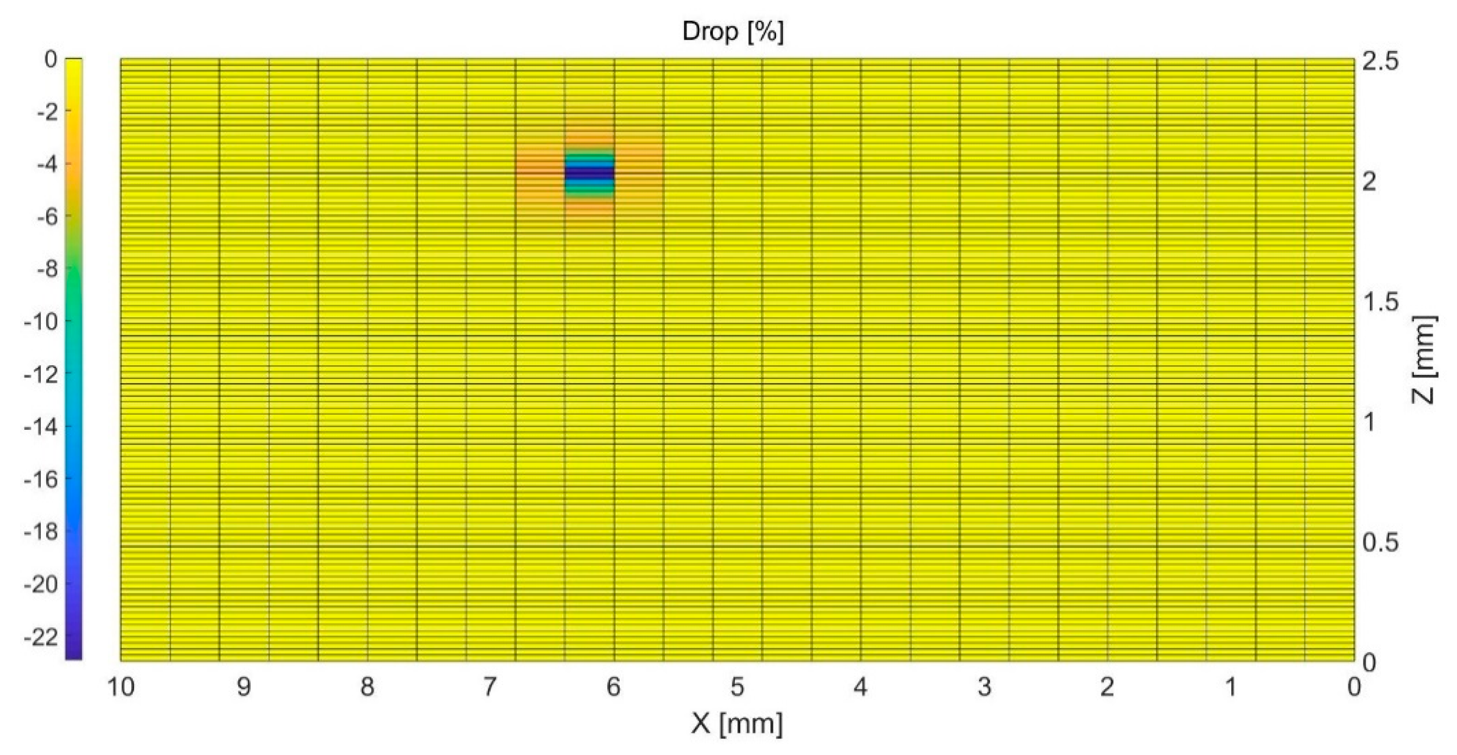
| Position (X, Z) (mm) | Depth from Topurface (mm) | Length (μm) | Reduction in (%) | |
|---|---|---|---|---|
| 1 | (6, 2) | −0.2 | 50 | 59 |
| 2 | (6, 2) | −0.2 | 100 | 100 |
© 2018 by the authors. Licensee MDPI, Basel, Switzerland. This article is an open access article distributed under the terms and conditions of the Creative Commons Attribution (CC BY) license (http://creativecommons.org/licenses/by/4.0/).
Share and Cite
Tserpes, K.; Kora, C. A Multi-Scale Modeling Approach for Simulating Crack Sensing in Polymer Fibrous Composites Using Electrically Conductive Carbon Nanotube Networks. Part II: Meso- and Macro-Scale Analyses. Aerospace 2018, 5, 106. https://doi.org/10.3390/aerospace5040106
Tserpes K, Kora C. A Multi-Scale Modeling Approach for Simulating Crack Sensing in Polymer Fibrous Composites Using Electrically Conductive Carbon Nanotube Networks. Part II: Meso- and Macro-Scale Analyses. Aerospace. 2018; 5(4):106. https://doi.org/10.3390/aerospace5040106
Chicago/Turabian StyleTserpes, Konstantinos, and Christos Kora. 2018. "A Multi-Scale Modeling Approach for Simulating Crack Sensing in Polymer Fibrous Composites Using Electrically Conductive Carbon Nanotube Networks. Part II: Meso- and Macro-Scale Analyses" Aerospace 5, no. 4: 106. https://doi.org/10.3390/aerospace5040106
APA StyleTserpes, K., & Kora, C. (2018). A Multi-Scale Modeling Approach for Simulating Crack Sensing in Polymer Fibrous Composites Using Electrically Conductive Carbon Nanotube Networks. Part II: Meso- and Macro-Scale Analyses. Aerospace, 5(4), 106. https://doi.org/10.3390/aerospace5040106