Improved Separation of Tone and Broadband Noise Components from Open Rotor Acoustic Data

Abstract

The term “open rotor” refers to unducted counter-rotating dual rotors or propellers used for propulsion. The noise generated by an open rotor is very complicated and requires special techniques for its analysis. The determination of its tone and broadband components is vital for properly assessing the noise control parameters and also for validating open rotor noise prediction codes. The data analysis technique developed by Sree for processing raw acoustic data of open rotors has been modified to yield much better results of tone and broadband separation particularly for the case when the two rotor speeds are approximately the same. The modified algorithm is found to eliminate most or all of the “spikes” previously observed in the broadband spectra computed from the original algorithm. A full description of the modified algorithm and examples of improved results from its application are presented in this paper.

1. Introduction

Renewed interest in counter-rotating open rotor technology for aircraft propulsion application (see References [1,2,3,4]) has prompted the development of advanced diagnostic tools for better design and improved acoustical performance. The term “open rotor” here refers to unducted counter-rotating dual rotors or propellers. The noise generated by an open rotor is very complex and needs special techniques for its analysis. The acoustic spectra from open rotor systems are known to be dominated by a profusion of tones, although the broadband component can also be a significant contributor to the total noise level [5]. The knowledge of individual noise levels of tone and broadband plays an important role in many noise reduction analyses. Thus, the determination of tone and broadband noise components is very important for properly assessing the noise control parameters and also for validating open rotor noise simulation codes [6,7].

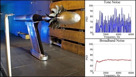
A signal processing technique was recently developed by Sree [1] to separate the tone and broadband noise components from open rotor acoustic data. To demonstrate its applicability, the technique was applied to simulated data as well as realistic acoustic data generated from a Himax hobby-aircraft open rotor, referred to as “mini-open rotor”, having four forward and three aft blades [1]. The technique was also applied recently to acoustic data generated from a 1/5th scale open rotor model, equipped with so-called “F31/A31” rotor blades in a 12-forward and 10-aft configuration, operating at realistic Mach numbers and tip speeds [8]. In both cases the two rotors were running at about equal speeds. Although reasonable separations of tone and broadband noise components were achieved in these two cases, the technique did not provide completely satisfactory results for certain datasets. It was found to result in non-trivial tone content still remaining in the broadband spectrum. The separated broadband spectra showed sharp “spikes” (or “blips”) at tone-dominated frequencies. (see, for example, Section 4.1. Specific cases of some of these results from the original algorithm will be included in Section 4 of this paper.) These spikes were significantly lower in amplitude than the corresponding tone levels. This implies that the acoustic power in tone or broadband was not being quantified properly. The limitations of the original technique have already been discussed by Sree [1], and Sree and Stephens [8].

In the data processing technique developed by Sree [1] the measured time series data is divided into uniform segments of a known number of samples and a cross-correlation operation is applied between two successive raw data segments to identify the phase shifts. These phase shifts in raw open rotor acoustic data are usually random and they occur due to jitter or unsteadiness in shaft rotations and other extraneous effects. The cross-correlation technique does not account for all the phase shifts that occur in a data segment-pair, it accounts only for the most dominant one (the accuracy of the phase shift determined using the cross-correlation is limited to discrete values of the sample time. The sample rate of the data should be much larger than the rate of drift of shaft phase. It seems as though this implies the method would only work on time-stationary data, but this has not been explored experimentally). After the dominant phase shift is determined, a phase-adjustment scheme is then applied to minimize the effect of the phase shift in the data segment-pair. It was demonstrated through use of simulated and realistic data (see [1,8]) that the presence of unresolved or unaccounted temporal phase shifts (or time lag) between the raw data segment-pairs contribute to “tone-like” spikes that appear in the broadband spectrum. A new way of processing the open rotor data had to be devised to minimize the effects of phase shifts and thereby eliminate the spike levels in the broadband spectrum. This continued search resulted in an improved method that involved a few modifications to the original technique. This improved method was found to work well for data from both single-shaft turbofan models and two-shaft counter-rotating propeller models with both shafts running at equal speed. Additionally, a separate study revealed that this new method works much better than the peak detection technique [5,9] in separating the tone and broadband components. Peak detection algorithms are inherently subjective, requiring either an expected spectral shape, peak height threshold, or other smoothing parameters. The user typically runs them multiple times, comparing the results against their expectations. It is not rigorous or mathematically well defined, hence not considered in this work.

The main purpose of this paper, therefore, is to present a description of the modified version of the original technique and to demonstrate its success through relevant examples. The same mini-open rotor data set used in [1] and a subset of the F31/A31 open rotor model datasets used in [8] will be again considered to make the comparisons and illustrate the improvements in tone and broadband separation. The emphasis will be on presenting improved results of tone and broadband separation rather than on technical details of experimentation and aeroacoustic characteristics of the open rotor models involved.

2. The Modified Algorithm

The original data processing technique by Sree [1] was based on combining cross-correlation and fast-Fourier transform (FFT) operations and was applied to separate the tone and broadband noise components from measured raw acoustic data of model open rotor systems. This technique, as stated earlier, has been modified to further minimize or eliminate the occurrences of unaccounted random phase shifts in the data segment-pairs. The modification involves choosing a shorter data segment size for the cross-correlation operation than the one previously used and then performing a reconstruction process of the ensuing broadband time series data. The idea here is that a shorter data segment-pair will have fewer occurrences of unaccounted random phase shifts compared to a longer one as previously used. A longer data segment-pair size is presumed to contain a relatively larger number of unaccounted phase shifts compared to a shorter one, thereby leading to more “spikes” to appear in the broadband spectrum. The shortest data segment size that will be considered in this study is the one which has samples equivalent to one shaft revolution long, i.e., data segment size ≈ number of samples per revolution (NPR). NPR will be a rounded off integer number. Depending upon the frequency resolution desired, an FFT window size, NFFT, is chosen and the FFT operation is finally performed on the reconstructed broadband data. It should be noted here that, in many instances the FFT window size (NFFT), which spans over several shaft revolutions, is much longer than the data segment size (NPR) chosen for the cross-correlation operation. This modification is found to yield improved results of tone and broadband separation, particularly when the two rotor speeds are approximately equal. The main difference here is that in the original algorithm by Sree [1] the data segment size chosen for the cross-correlation operation was of the same length as the desired window size for the FFT operation, i.e., both were of size NFFT.

The modified algorithm is similar to the original algorithm except for, as mentioned above, the selection of a shorter data segment size for the cross-correlation operation and the way the broadband signal is reconstructed. The differences between the modified and the original algorithms will be highlighted where appropriate. The steps involved in the modified algorithm are as follows:

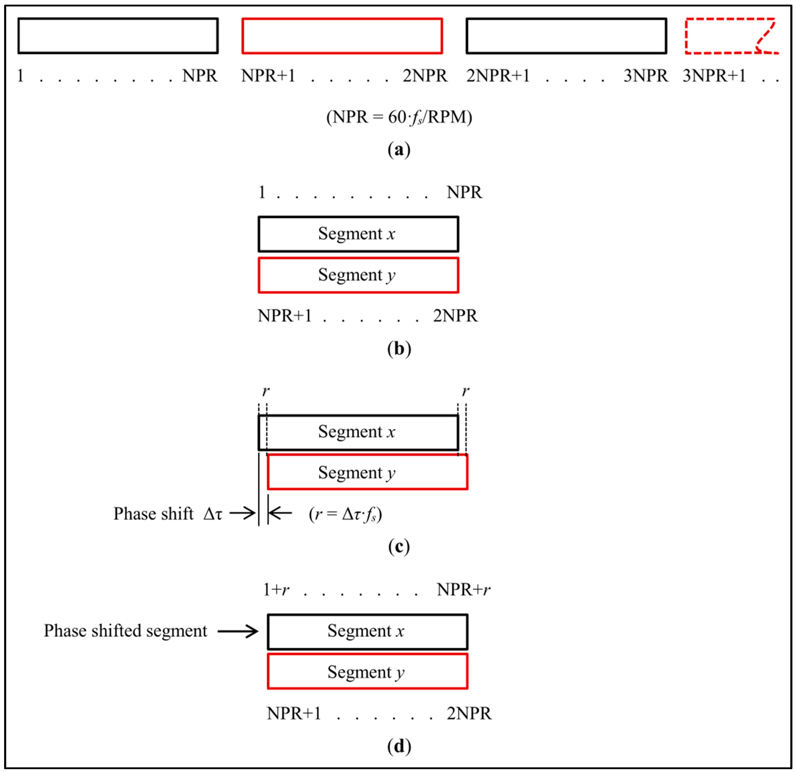
(1) Take a uniformly-sampled raw data set obtained at a given measurement location. The raw dataset here is termed the “total” signal. Starting from the beginning, divide this signal into small uniform time-series segments each containing NPR samples equivalent to one shaft revolution long, as depicted in Figure 1a.

The assumption here is that two consecutive rotations will be of very similar duration and have same number of samples. Note: NPR = 60·f_s/RPM, where f_s is the sampling frequency and RPM is the average shaft revolutions per minute. Thus, NPR depends on f_s and the average shaft RPM over the measurement duration. NPR would be different in different situations, but it has to be one revolution long when the two open rotor speeds are equal. It was found from several preliminary trials that a data segment size of nominally one shaft revolution long (NPR) would give the best results. The precise number of sample points in each revolution may change, but the next step accounts for the variation in rotor phase between the rotations. Breaking down the size to less than a revolution long, say, one-half of a revolution, did not yield any further improvement in the result. This “one-revolution long” segment choice seems fitting for the data generated from rotating systems, like open rotors. Selection of NPR when multi-shaft and unequal speeds are involved is a topic of further research and will be addressed in the future.

(2) Next, starting from the beginning, take two such consecutive data segments, say x and y (see Figure 1b), and perform the cross-correlation to determine the dominant phase shift, Δτ, between them (see Figure 1c). Δτ can be positive or negative depending upon whether x leads y or y leads x. Note this phase shift Δτ is equivalent to a shift of “r” number of samples given by r = Δτ·f_s. This r is typically a small number. The “xcorr” command in MATLAB, for example, can be used to perform the cross-correlation operation.

In the present study, large amplitude and low frequency background noise from the wind tunnel was found to affect the output Δτ. The low frequency noise was below the lowest frequency of interest from the open rotor and was removed using a digital band-pass filter 500 Hz–50 kHz (which spans a shaft order range of approximately 5 to 500).

(3) Then, phase-adjust one of the segments according to the sign of Δτ and align the two segments properly as illustrated in Figure 1d where segment y is shown to lead segment x by r samples. The matching or aligning of the two segments begins with shifting segment x to the right by r samples. The counting of samples for the shifted segment x now begins at 1 + r and ends at NPR + r, keeping the segment size at NPR always. To achieve this, the required r samples are borrowed from the original raw dataset after the NPRth sample sequentially (notice that these borrowed samples are nothing but those from the beginning of the segment y). This (1 + r)th sample or the first sample of the shifted segment x now must align with the first sample of segment y. Then the rest of the samples of the shifted segment x will automatically align with those of segment y. A similar phase adjustment procedure is followed if x leads y. Thus, each segment after phase adjustment must have the same sample size NPR.

(4) Note each segment is composed of a common tone component plus a unique realization of a stationary random component, i.e., x = $\overline{x}$ + x′ and y = $\overline{x}$ + y′. Being stationary in time, the two random components have the same statistics, $\overline{x^{\prime 2}}=\overline{y^{\prime 2}}$. This portion of the signal can be isolated by inverting one of the segments and combining them as: x + (−y) = $\overline{x}$ + x′ − $\overline{x}$ − y′ = x′ − y′. This cancels the tone portion of the signal, which is coherent between segment, but it amplifies the random portion of the signal, because that portion is incoherent between the segments and should be combined as mean-squared value, i.e.,:

$$\overline{{z^{\prime }}^2}=\overline{{x^{\prime }}^2}+\overline{{\left(-y^{\prime }\right)}^2}=2\overline{{x^{\prime }}^2}$$

to obtain the total broadband energy content in the data. Thus, by combining the two segments, the “broadband” signal, z’, can be computed as:

$$z^{\prime }=\frac{x-y}{\sqrt{2}}$$

It may be noted here that the broadband signal was determined slightly differently in the original algorithm through use of a common segment-averaged mean (z) [1,8]. Either method could be used to arrive at the desired broadband spectral result.

(5) Next, starting from the end of the first segment-pair, repeat steps 2 to 4 and get the second broadband signal similar to z′. Append this signal to the one previously found in step 4 to build a pseudo time-series of the broadband signal.

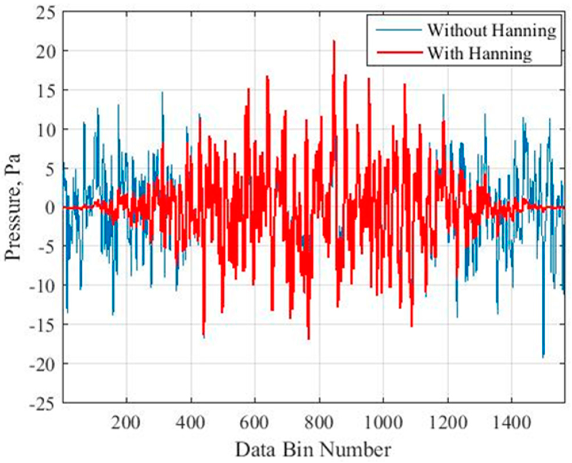
Appending the individual broadband segments will create discontinuity at each junction. This discontinuity can introduce a small amount of white noise into the computed spectrum. This noise can be mitigated using a smoothing window, such as Hanning [10], with each segment. Figure 2 shows a typical broadband data segment with and without Hanning applied. Note the beginning and the end points of each segment (NPR long) have zero values after Hanning. These zero end points allow smooth reconstruction of the signal without any discontinuity or overlap in it. The overall loss of energy (based on variance of the signal) because of Hanning is estimated to be less than one percent.

(6) Repeat steps 2 to 5 until all the segment-pairs in the original data set are taken into account and a long time-series of the broadband signal, which has no discontinuity in it, is reconstructed. Note the total length (or sample size) of this signal will be about one-half of that of the original raw data set considered for analysis. Hence, to use this modified algorithm it is suggested that at least one million samples be collected at each measurement location.

(7) Depending upon the frequency resolution (Δf) desired, draw NFFT samples from the reconstructed broadband pseudo-time series data sequentially for the FFT operation. Choosing a block size of NFFT gives Δf = f_s/NFFT in Hz. Perform the FFT operation on each block of data to obtain the broadband spectral values as a function of frequency. A Hanning window, for example, can be used to smooth the spectral estimates. FFT gives the spectral results from zero to Nyquist frequency, f_s/2. Drawing NFFT samples sequentially and performing the FFT operation results in “NBLKS_b” of broadband spectral data, where NBLKS_b = total sample size of the reconstructed broadband data divided by NFFT (see [10] for details on FFT operation and also cross-correlation). Note that the phase adjusting procedure (steps 2 and 3) was done to remove tones from the signal and, therefore, the reconstructed broadband signal should not have any tonal content. Thus, the NFFT block size and starting point can be arbitrary.

(8) Similarly, draw NFFT samples sequentially from the uniformly-sampled original raw acoustic data (note, this data has no discontinuity in it) and perform the FFT operation using a smoothing window on each block to obtain the “total” spectral values from zero to Nyquist frequency f_s/2 with the same Δf resolution. This results in “NBLKS_t” of “total” spectral data, where NBLKS_t = total sample size of original raw acoustic data divided by NFFT.

Note, steps 7 and 8 describe a method for calculating an estimated power spectrum. A packaged software tool such as MATLAB can be used to perform the FFT operation. The “pwelch” command in MATLAB, for example, performs this operation.

(9) Perform a frequency-wise averaging over “NBLKS_b” to obtain the final “broadband” spectral results and over “NBLKS_t” to get the final “total” spectral results, in the frequency range zero to f_s/2.

(10) Finally, subtract the “broadband” spectrum obtained in step 10 from the averaged “total” spectrum in step 8 to get the desired “tonal” spectrum.

It should be pointed out that the modified algorithm includes averaging in both the time and frequency domains. It is believed that this is a relatively unusual approach. Combining the two techniques (phase-adjusted temporal averaging and frequency domain spectral averaging) is one reason why this method is successful. This method was found to work well for many different input sets of data from both single-shaft turbofan models and the two-shaft counter-rotating propeller models.

3. Validation of the Modified Algorithm against Phase-Averaging

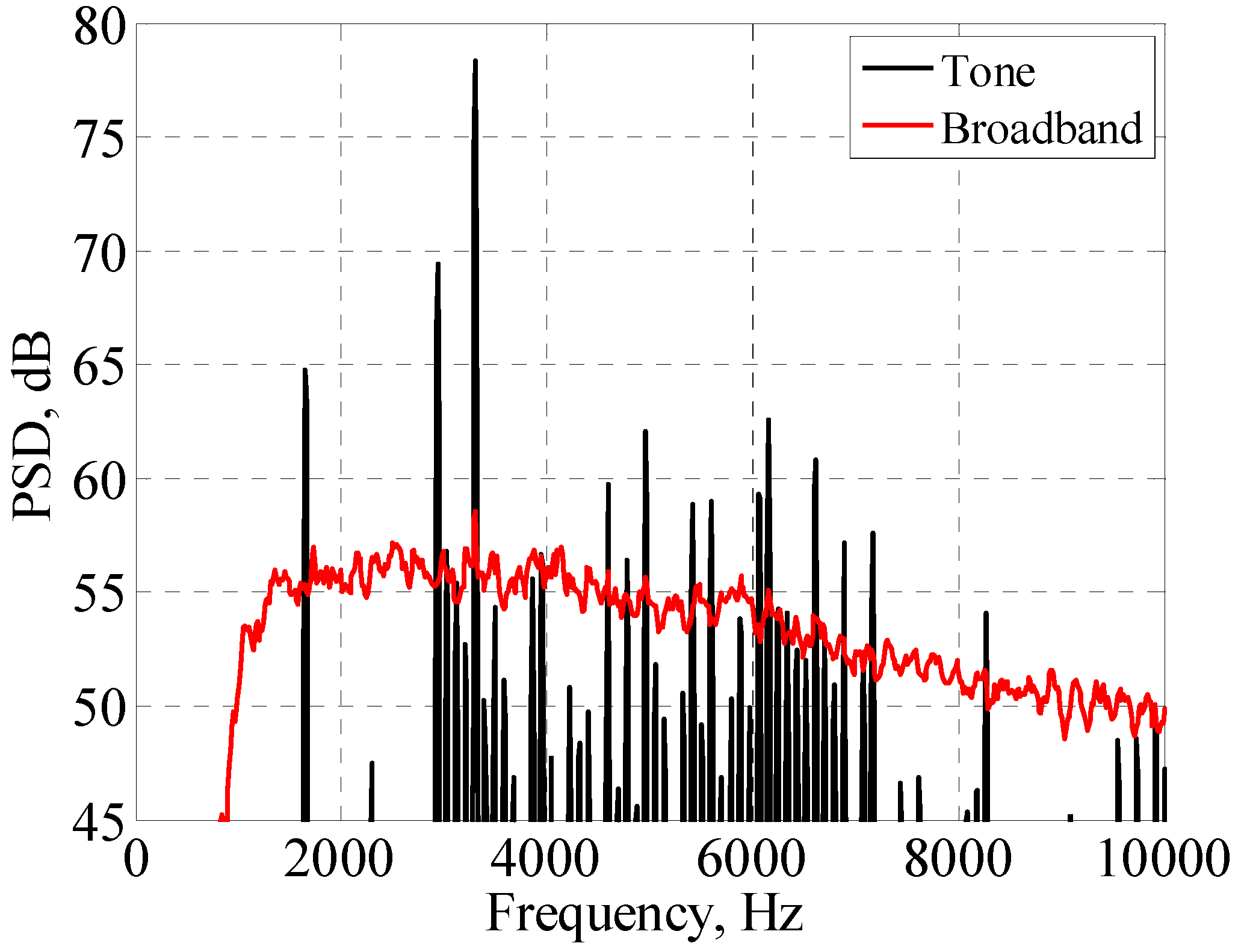
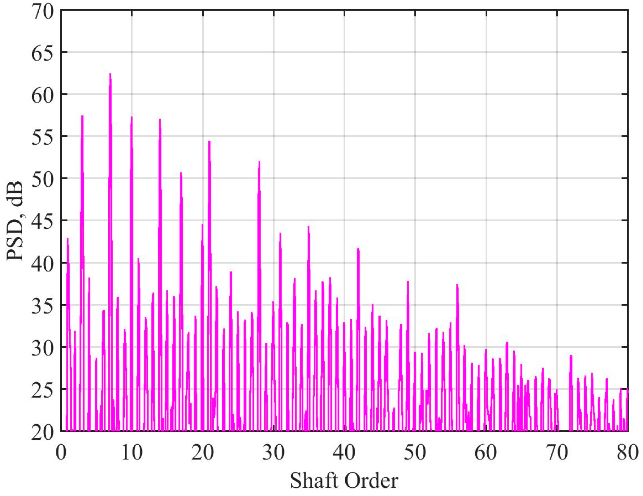
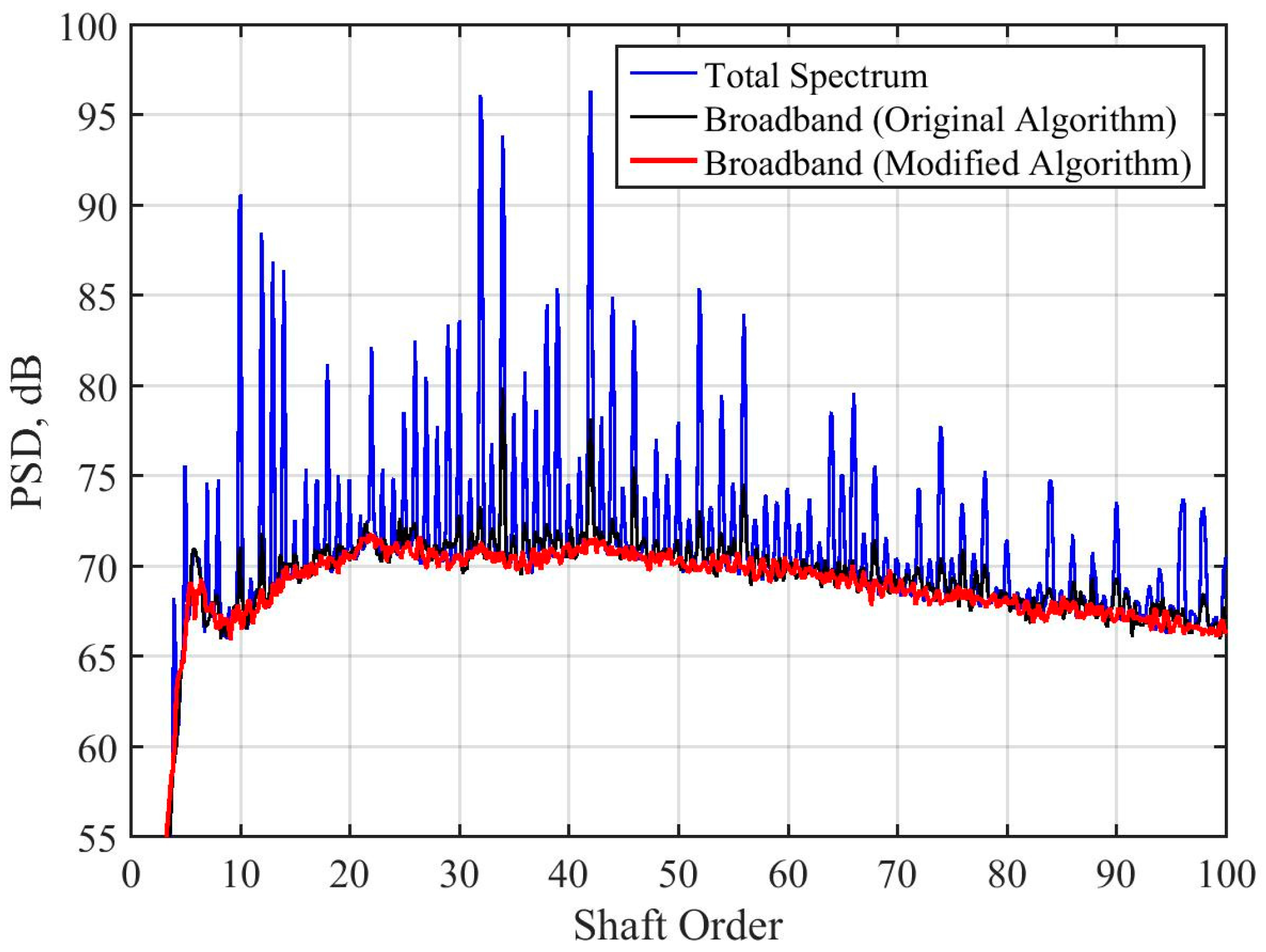
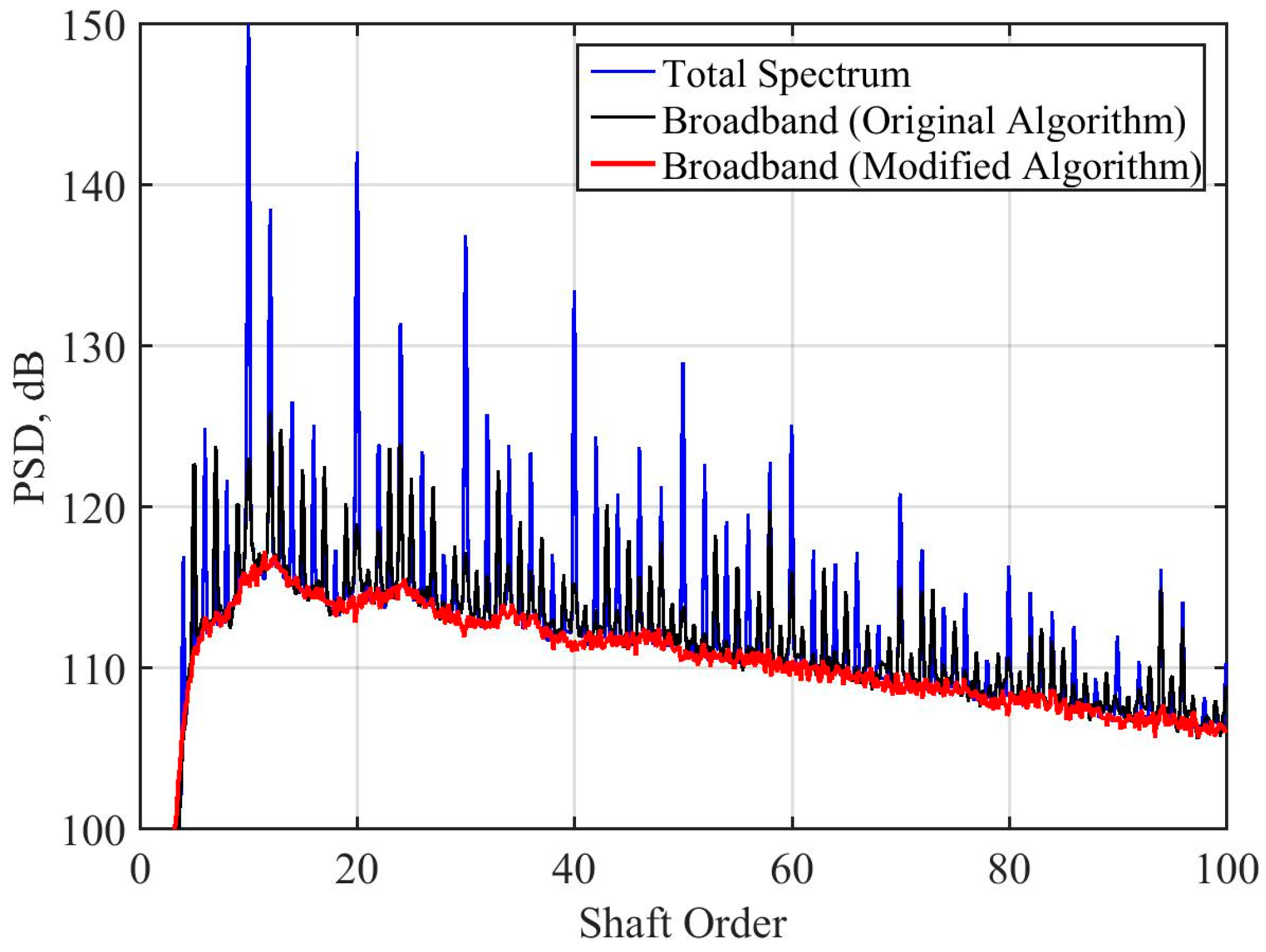
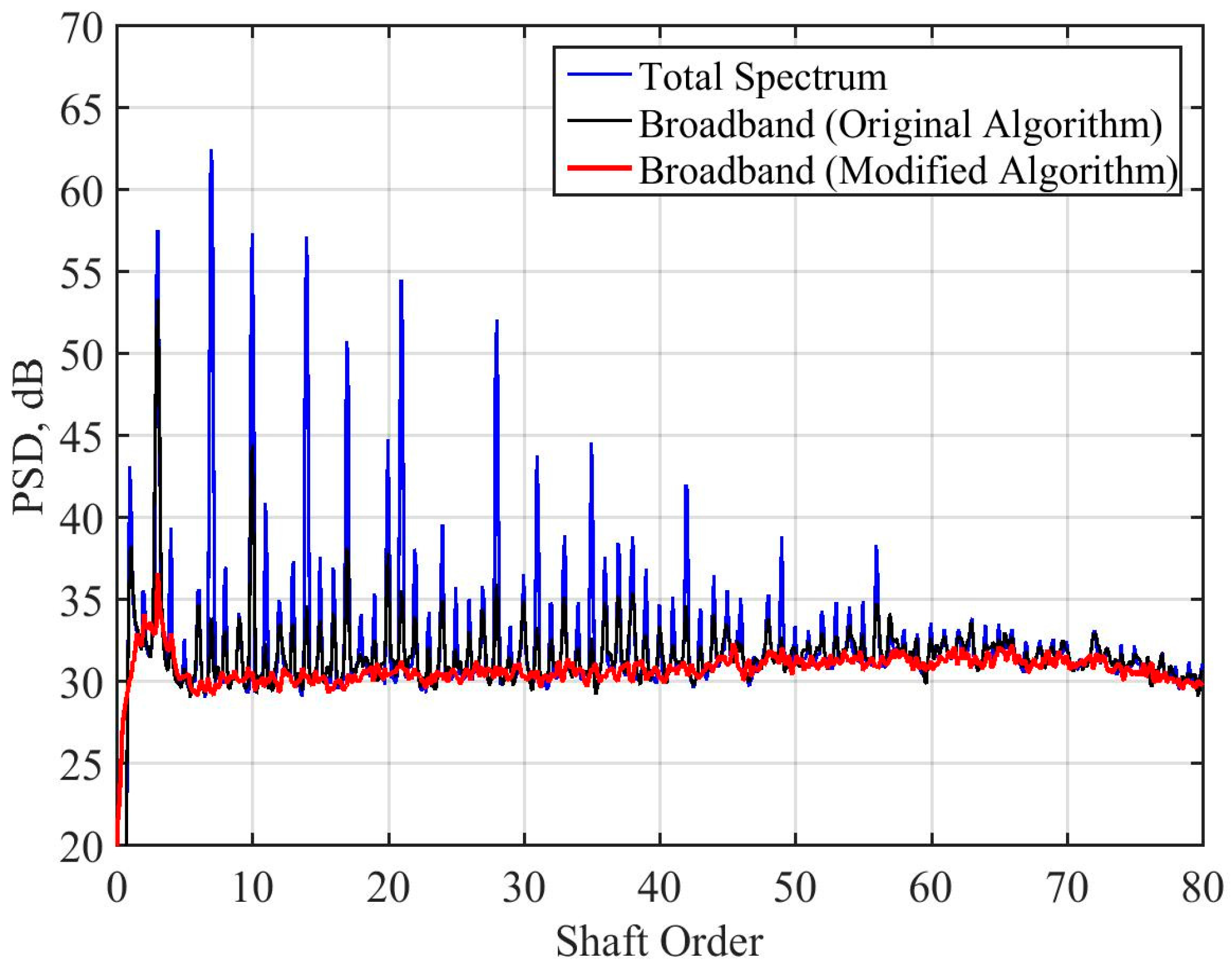
The most well-defined description of the tone portion of a signal from a rotating machine is that which is periodic with the shaft rotation. Phase-averaging is known to work well for single-shaft systems, but is ill-defined and, hence, does not work well for processing noise from multi-shaft systems, as discussed in [1,8]. In phase-averaging, the shaft phase is calculated by using a once-per-revolution trigger, which is sampled simultaneously with the microphone signal. This gives the shaft phase angle for each sample in the microphone time series. The microphone time series is then interpolated onto a new shaft phase vector with equal spacing in shaft phase. Then the average microphone pressure value at each shaft phase can be calculated, giving a periodic function that is called the “phase average”. This function contains all the energy in the signal that is coherent with shaft phase. This function can be repeated as many times as needed to make a time series of length equal to that of the original signal, which can then be subtracted from the original signal to give a time series of broadband energy. 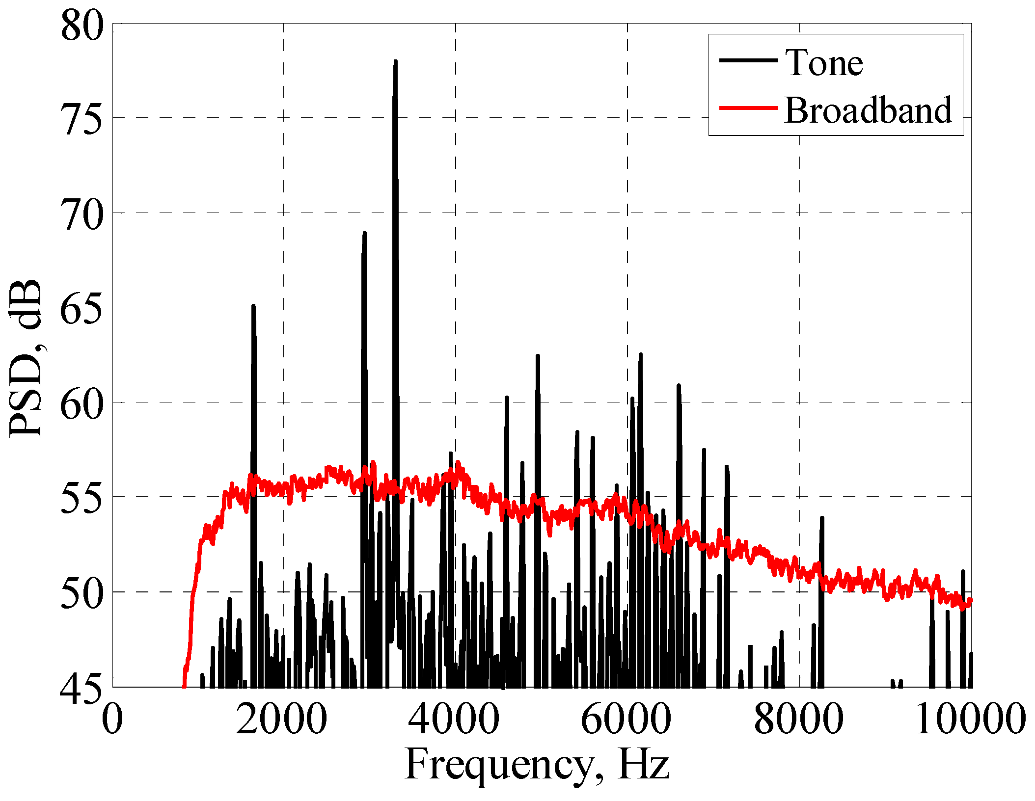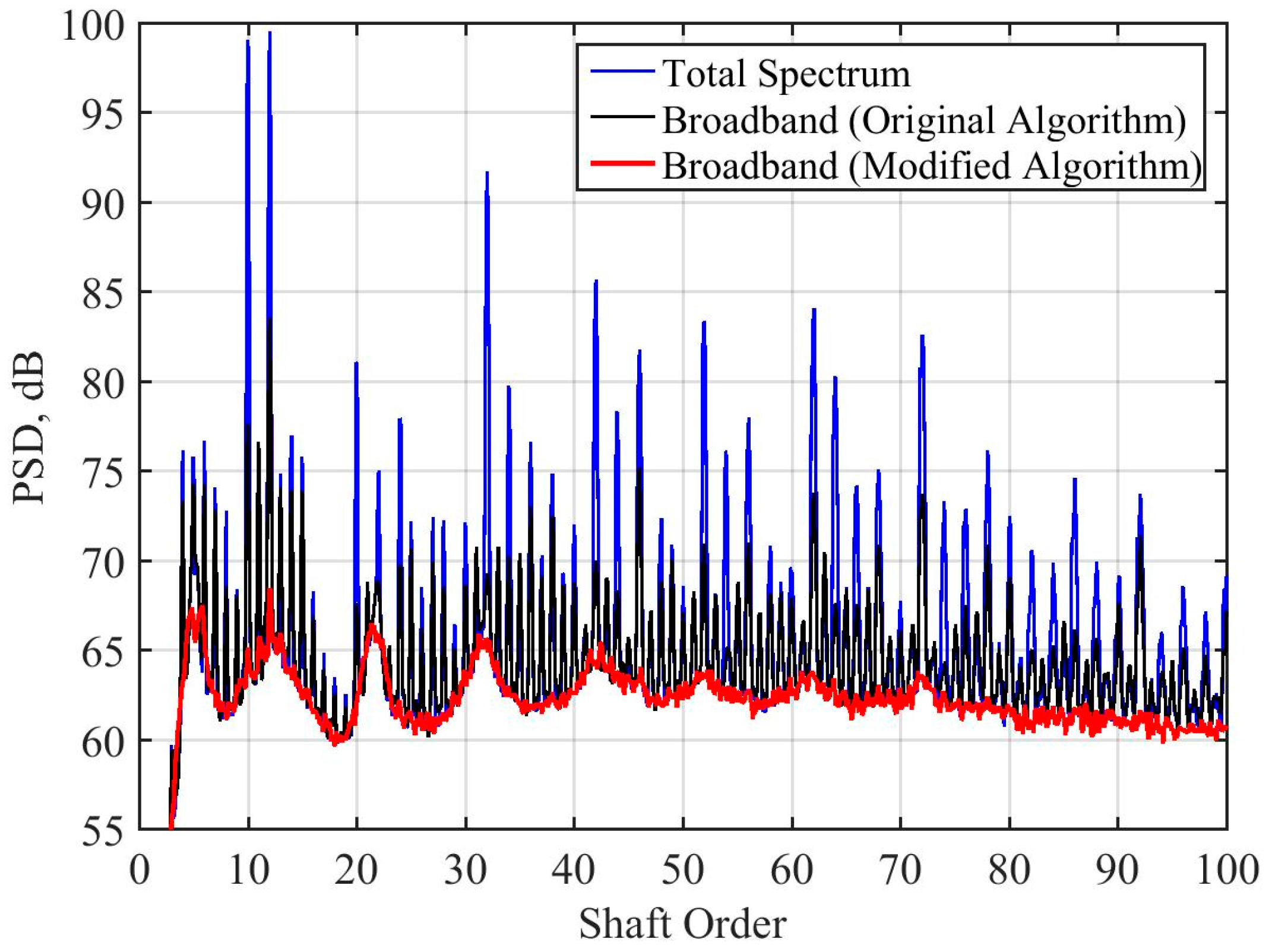The noise levels, in terms of power spectral density (PSD, in decibels (dB), referenced to 20 micro-Pascals) as a function of frequency (in Hz), can be calculated from both of these signals, giving the result shown in Figure 3 for a single-shaft model turbofan. The results from the modified algorithm using the same data are shown in Figure 4.

The broadband spectra in these two figures seem to agree pretty well. However, residual tone components extracted from the modified algorithm are higher in number and appear noisy, but are lower in amplitude. The residual tones found in Figure 4 occur at multiples of the shaft rate, but evidently do not repeat perfectly with each fan rotation and so are excluded from the phase average result.

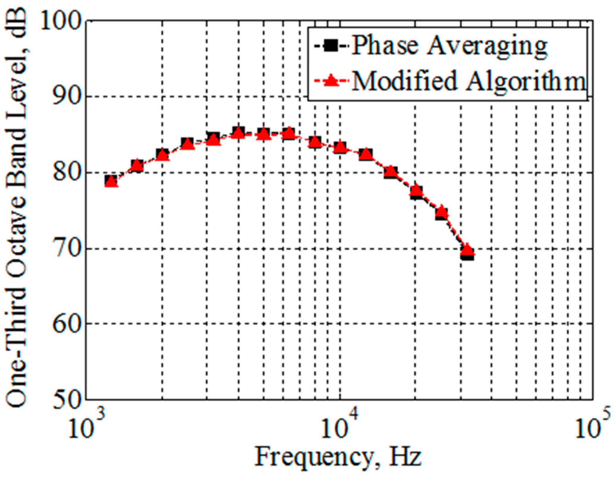
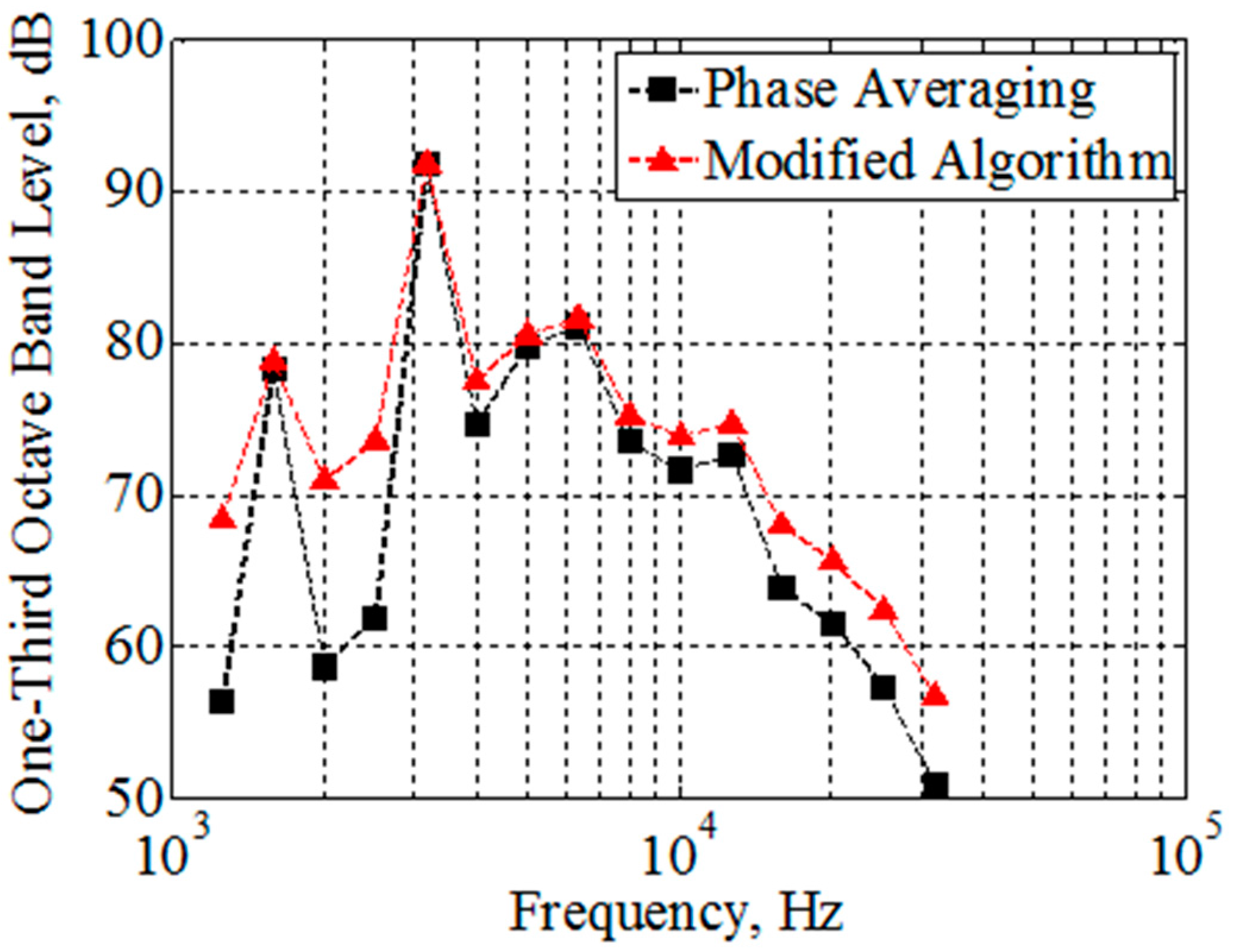
A comparison of one-third octave band levels of the broadband spectra from the two methods for the same fan data are also shown in Figure 5, and that of tone spectra in Figure 6. These were computed by integrating the narrow-band spectra of Figure 3 and Figure 4 across each one-third octave band. It is noticed that the two broadband spectra in Figure 5 seem to agree very well (within 0.6 dB) across the frequency range. Figure 6 shows that the one-third octave bands containing tones that are as much as 5 dB below the broadband also agree well. In the one-third octave bands that do not contain tones or when the tone level is more than 5 dB below the broadband (2000 Hz for example) the extra tone components extracted by the modified algorithm lead to levels that are higher than those from the phase-averaging method.

Quantitatively these results can be compared by integrating each curve in Figure 3 and Figure 4 over frequency to get the overall tone and broadband sound power levels found using each method. These results were calculated and are shown in

Table 1. Integrated tone and broadband spectral levels for the model turbofan.

Noise Component	Phase-Averaging (dB)	Modified Algorithm (dB)
Broadband	94.43	94.33
Tone	92.77	93.16

. The results indicate a good agreement between the two methods, with only about 0.1 and 0.39 dB difference for the broadband and tone portions, respectively. The broadband spectra se two figures seem to agree rather well.

4. Open Rotor Test Cases and Discussion

In order to test and demonstrate the applicability of the modified algorithm, four different cases are considered here. As mentioned earlier, acoustic data generated from the mini-open rotor [1] and 1/5th scale F31/A31 open rotor model [8] are utilized for the study. A description of mini-open rotor model and details of acoustic data generation with it are given in [1]. The F31/A31 model description and details of the experiments with it in the low- and high-speed tunnels at NASA Glenn Research Center (GRC) can be obtained from [11,12,13]. The spectral results from both the original and the modified algorithms are used to make the comparisons and validate them. Only relevant information necessary for validation of the modified algorithm will be given here. In each example, the sampling frequency, frequency resolution, FFT block length, total sample size, and other related parameters will be kept the same so that valid comparisons can be made between the two algorithms. The data segment size for the cross-correlation operation and the window size for the FFT operation were both equal in the original algorithm whereas they are different in the modified algorithm. The data segment size for the cross-correlation operation in the modified algorithm will be NPR, equivalent to about one shaft revolution long. The FFT window size depends on the frequency resolution desired. In both algorithms the MATLAB commands “xcorr” and “pwelch” were used for the cross-correlation and FFT operations, respectively.

4.1. Case 1: Data from Mini-Open Rotor

The far-field acoustic (unsteady pressure) data from the mini-open rotor were obtained from an azimuthal sideline microphone 1.524 m (5 ft) away from the model center using a sampling frequency of 50 kHz. A 100 Hz–10 kHz band-pass filter was used to cutoff unwanted noise. Both rotors were spinning at approximately the same speed of 6740 RPM. The speed variation between the aft and the forward rotors was found to be less than one percent and that between successive shaft rotations even less. Data analysis was carried out using both the original and the modified algorithms. A data segment size of 4096 samples was used for the cross-correlation process in the original algorithm whereas it was 445 (NPR) in the modified algorithm for the same purpose. A window size of NFFT = 4096 samples, which gives a frequency resolution of 12.2 Hz, and a total sample size of 1 million were used for the FFT analysis in both algorithms.

The noise spectral results, in terms of power spectral density (PSD), in dB, from the original and the modified algorithms are presented in Figure 7, where the frequency axis is given in terms of shaft order (SO), so that the blade-rate tones and the interaction tones can be visualized easily. SO is defined as: SO = f/RPS, where f is frequency, in Hz, and RPS is shaft rotation in revolutions per second. The shaft orders of expected tones for the mini-open rotor are calculated as sums of integer multiples (m and n) of four forward and three aft blade counts, i.e., SO(m,n) = 4m + 3n, when the shaft speeds are equal [8]. The “blade-rate tones” occur at expected shaft orders when either m or n is zero. Tones at shaft orders when m and n are both non-zero are called the “interaction tones”. These expected shaft order tones up to m = n = 6 for the mini-open rotor are tabulated as shown in

Table 2. Expected shaft order tones for 4 × 3 mini-open rotor with equal rotor speeds.

Order	n = 0	n = 1	n = 2	n = 3	n = 4	n = 5	n = 6
m = 0		3	6	9	12	15	18
m = 1	4	7	10	13	16	19	22
m = 2	8	11	14	17	20	23	26
m = 3	12	15	18	21	24	27	30
m = 4	16	19	22	25	28	31	34
m = 5	20	23	26	29	32	35	38
m = 6	24	27	30	33	36	39	42

below.

It can be seen in Figure 7 that the spectral results obtained using the modified algorithm are clearly better than those from the original algorithm, in relation to tone and broadband separation. The blade-rate tones as well as the interaction tones at expected shaft orders are nicely resolved. Particular attention is given to broadband noise separation in the present context. The broadband spectrum from the original algorithm (black) is found to have many narrow band features (“spikes”) remaining at frequencies that had strong tones in the total signal spectrum, whereas the modified algorithm returns a broadband spectrum (red) that is very “clean” and it is practically free of the spikes. This improvement is believed to be because of a shorter data segment size (445 samples) used for the cross-correlation operation in the modified algorithm compared to 4096 samples (9.2 times longer) in the original algorithm. As previously mentioned, longer data segments tend to have more unaccounted random phase shifts that go undetected. Note, as mentioned before, the cross-correlation operation does not account for all of the phase shifts that occur in the data segment-pair, it accounts only for the most dominant one. The more the random phase shifts there are, the more the number of spikes will be in the broadband spectrum. It should also be realized here that the modified algorithm resembles more like the phase-averaging principle (without any need of a tachometer signal to track shaft rotation). Therefore, the phase compensation of consecutive data segments, each NPR long, causes a compensation also for small speed-variability among different segments of the whole signal, thus providing better results.

For a better understanding and visualization of the output from the modified algorithm, the tone noise spectrum is plotted in Figure 8. This spectrum is the difference between the “total” spectrum (blue) and the “broadband” spectrum (red) shown in Figure 7. This spectrum has clear separation between the tones and is useful for quantifying the level of individual tones, or of particular tones together.

A quantitative comparison between the outputs can be made using the overall sound pressure level (OASPL) metric. This is computed from the narrowband spectrum by integrating over all frequencies, or over particular frequencies of interest. Considering the results from the modified algorithm to be “correct”, the original algorithm over-predicts the broadband OASPL by 2.2 dB while under-predicting the tone level by 0.4 dB.

4.2. F31/A31 Open Rotor Data

The one-fifth scale F31/A31 blade set serves as a non-proprietary baseline design for comparison with the advanced open rotor blade designs tested during a recent wind tunnel campaign [14]. Far-field sideline acoustic (unsteady pressure) measurements of this model at simulated approach and nominal takeoff conditions were performed in the NASA GRC 9’ × 15’ low-speed wind tunnel (LSWT) using a traversing microphone probe on a track parallel to and 1.524 m (5 ft) away from the model longitudinal axis. Data were taken at 18 fixed positions as the traverse moved from the rear to the front side of the model during each test run at a freestream Mach number of 0.2 [13]. Tests were also conducted in the NASA GRC 8’ × 6’ supersonic (high-speed) wind tunnel (SWT) to obtain near-field sideline acoustic data at simulated cruise conditions with freestream Mach numbers ranging from 0.27 to 0.85. Simultaneous acoustic measurements were made using 17 inline sensors mounted on an overhead plate. The near-field distances varied from 42.6 cm (16.8 inches) to 116.1 cm (45.7 inches) [12].

In both the LSWT and SWT tests the two rotors were running at equal speeds and the blade pitch angles were set optimum for a given flight condition. The speed variation between the two rotors of the F31/A31 model was less than one percent and that between successive shaft rotations much less [8]. In most cases the model was positioned at 0° angle of attack in the tunnel. The acoustic data were obtained at a sampling frequency of 200 kHz. Before carrying out the data analysis, the data were pre-processed using a 500 Hz–50 kHz band-pass filter to cutoff unwanted noise. This puts the frequency range of interest up to 50 kHz, although FFT gives results up to 100 kHz. An FFT block size of NFFT = 16,384, which gives a frequency resolution of 12.2 Hz, and a sample size of 3 million were used for computing the spectral results from both algorithms. Three cases, each representing a given simulated flight condition, are considered here to compare and validate the spectral results from the modified algorithm. The simulated approach case is considered first and then the simulated takeoff and cruise cases.

4.2.1. Case 2: Data from Simulated Approach Condition

The dataset considered here is the same one used in [8] and was obtained from a microphone positioned at a sideline distance of 1.524 m and 90° geometric directivity angle, with both rotors running at an average speed of 7668 RPM. This dataset is of particular interest because the original algorithm did not provide very satisfactory results [8].

The spectral results (PSD, in dB, vs. SO) for this case are shown in Figure 9 (the results are shown up to a shaft order of 100 (~12.8 kHz) only because bulk of the model tones was within this range). The computed broadband spectrum from the original algorithm is shown in black and that from the modified algorithm in red. The “total” spectrum from the raw data is shown in blue. A data segment size of 16,384 samples was used for the cross-correlation operation in the original algorithm, whereas it was 1564 (NPR) in the modified algorithm, which is about 10.5 times shorter.

It is clear from Figure 9 that the results obtained from the modified algorithm are excellent compared to those from the original algorithm. The broadband spectrum (red) from the modified algorithm is virtually free of the “spikes” found in the broadband spectrum (black) from the original algorithm. The blade-rate tones and the interaction tones (not plotted) were also nicely resolved. The modified algorithm provides a much better broadband separation for the same reasons explained while discussing the mini-open rotor case in Section 4.1, i.e., choosing a shorter data segment for the cross-correlation operation helps remove most of the “broadband spikes” compared to a longer data segment.

The expected shaft order tones up to m = n = 6 for the F31/A31 open rotor model are tabulated as shown in

Table 3. Expected shaft order tones for a 12 × 10 F31/A31 model with equal rotor speeds.

Order	n = 0	n = 1	n = 2	n = 3	n = 4	n = 5	n = 6
m = 0		10	20	30	40	50	60
m = 1	12	22	32	42	52	62	72
m = 2	24	34	44	54	64	74	84
m = 3	36	46	56	66	76	86	96
m = 4	48	58	68	78	88	98	108
m = 5	60	70	80	90	100	110	120
m = 6	72	82	92	102	112	122	132

. It is noticeable that the broadband spectrum returned by the modified algorithm does have a complicated shape with several local maxima around SO = (m = 1, n), i.e., 12, 22, etc. perhaps due to spectral broadening which happens when sound travels through the shear layer to the far microphone. This may also be due to unsteadiness in the wake of the front rotor which causes a non-uniform distribution of turbulence length scales to impinge on the aft rotor. It is interesting to notice here that the modified algorithm is able to detect these broadband peaks successfully.

4.2.2. Case 3: Data from Simulated Nominal Takeoff Condition

The dataset considered here is the same one used in [8]. The data were obtained from a sensor at the same location mentioned in Case 2. The rotors were running at an average speed of 6487 RPM. The computed total spectrum (blue) and the broadband spectra for this case are shown in Figure 10. The broadband spectrum from the original algorithm is shown in black and the one from the modified algorithm in red. The data segment size for the cross-correlation operation was 16,384 in the original algorithm and 1849 (about 8.9 times shorter) in the modified algorithm.

This is a situation where the original algorithm performed rather well, but it is obvious from the comparison of the results in Figure 10 that the modified algorithm performs better than the original algorithm. The blade-rate and the interaction tones of the model (refer to Table 3) are well resolved. The broadband spectrum (black) from the original algorithm had spikes at SO = 34, 44, and 46, while the broadband spectrum (red) from the modified algorithm is “clean” and free of spikes. Clearly, the modified algorithm outperforms the original one for the same reasons discussed earlier, i.e., selection of a shorter data segment for the cross-correlation operation helps improve the tone and broadband noise separation from the measured open rotor raw acoustic data.

4.2.3. Case 4: Data from Simulated Cruise Condition

The dataset considered for this example is the same one used in [8]. The acoustic data were obtained from a sensor directly above and 50.8 cm (20 in) away from aft rotor center. Both rotors were running approximately at 6943 RPM. The freestream Mach number was 0.78. This case is of particular interest because of the close proximity of the sensor to the rotors and also because of a different operating condition compared to the last two examples.

The spectral results, i.e., the “total” spectrum (blue) and the broadband spectra from the original algorithm (black) and the modified algorithm (red), for this case are shown in Figure 11. For the cross-correlation process, the data segment size selected in the original algorithm was 16,384 samples and it was 1728 (about 9.5 times shorter) in the modified algorithm.

It is again clear from Figure 11 that the modified algorithm provides a much better result than the original algorithm. The blade-rate and the interaction tones (refer to Table 3) are well resolved. As expected, the broadband spectrum (red) from the modified algorithm is “clean” and is free of a profusion of spikes found in the broadband spectrum (black) from the original algorithm.

5. F31/A31 Data Statistics

To better quantify the improvement in the data processing method, the overall sound pressure level (OASPL) of tone and broadband noise for the F31/A31 datasets were calculated. Considering both the approach and takeoff conditions in the low-speed test, 53 different configurations were tested, including some cases with a pylon installed upstream of the rotors and some cases with the rig at an angle of attack to the wind tunnel centerline. Each configuration was measured at 18 different sideline angles for a total of 954 recordings. Similarly, the high-speed test considered 222 conditions (combinations of blade pitch angles, free-stream Mach numbers and sensor plate stand-off distances) and 17 sensors, totaling 3774 recordings. All of these readings were run through both algorithms, the narrowband spectra were integrated in frequency to give the OASPL, and the results are given in

Table 4. Differences in overall sound pressure level (OASPL) of tone and broadband noise of F31/A31 model computed using the spectral results from original and modified algorithms.

Test Type	Noise Component	Maximum Overestimation (dB)	Maximum Underestimation (dB)	Mean Difference (dB)
Low-speed	Broadband	4.40	−0.21	0.84
	Tone	−0.02	−2.12	−0.25
High-speed	Broadband	4.03	−0.20	0.54
	Tone	−0.01	−3.28	−0.97

. The most obvious problem with the original algorithm is that it left too much energy in the “broadband” spectra, as shown in Figure 9, Figure 10 and Figure 11 above. This resulted in too little energy left in the “tone” spectra. During the low-speed portion of the F31/A31 test, the broadband OASPL was overestimated by up to 4.4 dB, with the tone OASPL underestimated by up to 2.1 dB. The mean differences are smaller, but still up to about +/− 1 dB.

6. Conclusions

The determination of tone and broadband components of complex noise generated by open rotors is important for properly assessing the noise control parameters and also for validating the open rotor noise prediction codes. The original technique developed by Sree [1] for separating the tone and broadband noise components from raw acoustic data of open rotors had some drawbacks. It did not provide a clean separation of these components. The computed broadband spectrum contained irregular tone-like “spikes” due to unaccounted random phase shifts occurring in the long data segment-pairs selected for the cross-correlation operation. This problem is mitigated through selection of short (one shaft revolution long) data segment-pairs in the modified algorithm. The modified algorithm, fully described in this paper, is shown to provide excellent results of tone and broadband noise separation from raw acoustic data generated by open rotors. Four test cases were considered to demonstrate the improvement of the results from the modified algorithm over the original algorithm. The modified algorithm is shown to perform well when the two rotor speeds are approximately equal. It will be interesting to see how well this algorithm will perform when the two speeds are unequal or when more than two shafts running at different speeds are involved. Lastly, the modified algorithm can also be used for processing acoustic or flow data from single rotors such as fans or propellers, without requiring a shaft position signal.