Safety-Guaranteed Go-Around Decision Framework Based on Funnel for Automatic Carrier Landing Systems

Abstract

Existing go-around decision methods for Automatic Carrier Landing Systems (ACLSs) are mainly based on altitude deviation. The safe region implied by these methods is therefore effectively single-dimensional, which can lead to overly conservative and incomplete go-around decisions because the remaining state deviations are not evaluated. This paper proposes a safety-guaranteed go-around decision framework based on a funnel that explicitly characterizes the time-varying safe region in the multi-dimensional state space throughout the landing process, thereby enabling safe and precise decisions. A six-dimensional funnel is then computed backward from the terminal set using sum-of-squares programming while accounting for nonlinear dynamics, actuator saturation constraints, and prescribed bounded uncertainties. The resulting funnel guarantees that all closed-loop trajectories initialized within it remain within the subsequent funnel and reach the terminal set at the final time. In the online stage, the online go-around decision module evaluates at each sampling instant whether the complete six-dimensional state deviation lies inside the corresponding precomputed funnel and outputs either the continue-landing decision or the go-around decision. Simulation results show that incorporating the range state reduces the mean, maximum, and standard deviation of the terminal altitude deviations by approximately 68%, 64%, and 66%, respectively, and the corresponding statistics of the terminal range deviations by approximately 99%. Under a representative deck-motion disturbance, the framework remains effective after the six-dimensional funnel is recomputed offline. The proposed method also avoids unnecessary go-around decisions when the altitude component exceeds the conventional threshold but the complete six-dimensional state deviation remains inside the funnel.

1. Introduction

Carrier landings are considerably more hazardous than conventional land-based landings. Their failure rate is substantially higher, and landing-related accidents account for the majority of total mishaps in carrier aviation, underscoring the critical need for safe automatic carrier landing to support future naval aviation [1,2].

Making safe and precise go-around decisions requires an explicitly characterized safe region, whereas existing methods are mainly based on altitude deviation. In these methods, a nominal trajectory is precomputed, and the current altitude deviation is compared with a prescribed altitude-deviation threshold to determine whether a go-around should be initiated during landing [3]. Such a criterion is straightforward to implement online because it requires only a single state deviation and a prescribed threshold. However, this simplicity comes at the cost of not directly evaluating the coupled effects of the remaining state deviations in the go-around decision criterion. Specifically, an altitude deviation outside the prescribed threshold does not necessarily imply that the complete six-dimensional state deviation lies outside the safe region, whereas an altitude deviation within the threshold does not guarantee that the remaining state deviations are compatible with the actuator saturation constraints and terminal landing requirements. Therefore, a single-dimensional criterion cannot fully determine whether all landing-task requirements can still be satisfied and may lead either to unnecessary go-around decisions or to continue-landing decisions without a complete-state safety basis.

In this paper, the safe region is characterized as the set of complete six-dimensional state deviations from which, under the closed-loop dynamics and prescribed uncertainty bounds, the subsequent closed-loop trajectory is guaranteed to remain within the corresponding time-varying funnel throughout the landing process, satisfy the actuator saturation constraints, and reach the terminal set reflecting the required landing precision at the final time. Environmental disturbances are treated as one type of uncertainty within this framework. Conventional carrier-landing go-around decision methods are commonly formulated using simplified longitudinal aircraft dynamics. In particular, representative methods based on small-disturbance dynamics and terminal-state prediction estimate the aircraft altitude at the carrier stern and determine the go-around decision according to the prescribed go-around boundary [3]. Consistent with this established modeling practice, this study adopts a nonlinear longitudinal model and extends the decision basis from altitude deviation alone to the complete six-dimensional longitudinal state. By jointly evaluating the airspeed, flight-path angle, pitch angle, pitch rate, altitude, and range deviations, the proposed six-dimensional rule accounts for the coupled effects of the complete longitudinal state while retaining a simple scalar membership test during online implementation. Therefore, a more appropriate go-around decision rule should evaluate the complete six-dimensional state deviation rather than the altitude deviation alone.

In addition, making safe and precise go-around decisions in ACLSs still faces three major challenges [2]: (1) Complex nonlinear dynamics. Unlike rotorcraft [4], fixed-wing carrier aircraft must handle strongly coupled nonlinear aerodynamic effects and complex flight dynamics. (2) Stringent required landing precision. The desired landing area—approximately ±22.65 feet longitudinally and ±20 feet laterally [5]—is substantially more limited than the conventional land-based landing area. (3) Severe environmental disturbances. Atmospheric turbulence and deck motion introduce significant time-varying disturbances that challenge flight stability and control robustness. To address these challenges, existing ACLS control methods can be broadly classified according to their design mechanisms. Classical control approaches include PID control [6] and robust control [7]. Nonlinear control methods, particularly dynamic inversion and backstepping control, have been introduced to better accommodate the nonlinear aircraft dynamics [8]. Robustness-oriented approaches, including adaptive control, adaptive sliding-mode control, active disturbance rejection control, and neural-network-based disturbance observers, have been developed to mitigate the effects of uncertainties and environmental disturbances [9,10,11,12,13,14,15]. Prescribed-performance control, fixed-time control, and control-barrier-function-based control have also been investigated to constrain tracking errors during carrier landing [16,17,18,19]. In practical ACLS designs, several of these techniques are often integrated into composite control architectures [7,10,14,15,16,17,18,19,20,21,22,23]. In addition, feedforward–feedback composite approaches, including preview control and model-predictive-control formulations such as output-feedback stochastic MPC and receding-horizon control, have been studied to improve landing performance and adaptability [3,24,25,26,27,28]. Although these methods improve trajectory-tracking accuracy and robustness, they primarily act on the guidance and control system rather than modifying the go-around decision criterion itself. Consequently, the decision may still be based on altitude deviation and does not explicitly determine whether the complete six-dimensional state deviation can satisfy the actuator saturation constraints and terminal landing requirements.

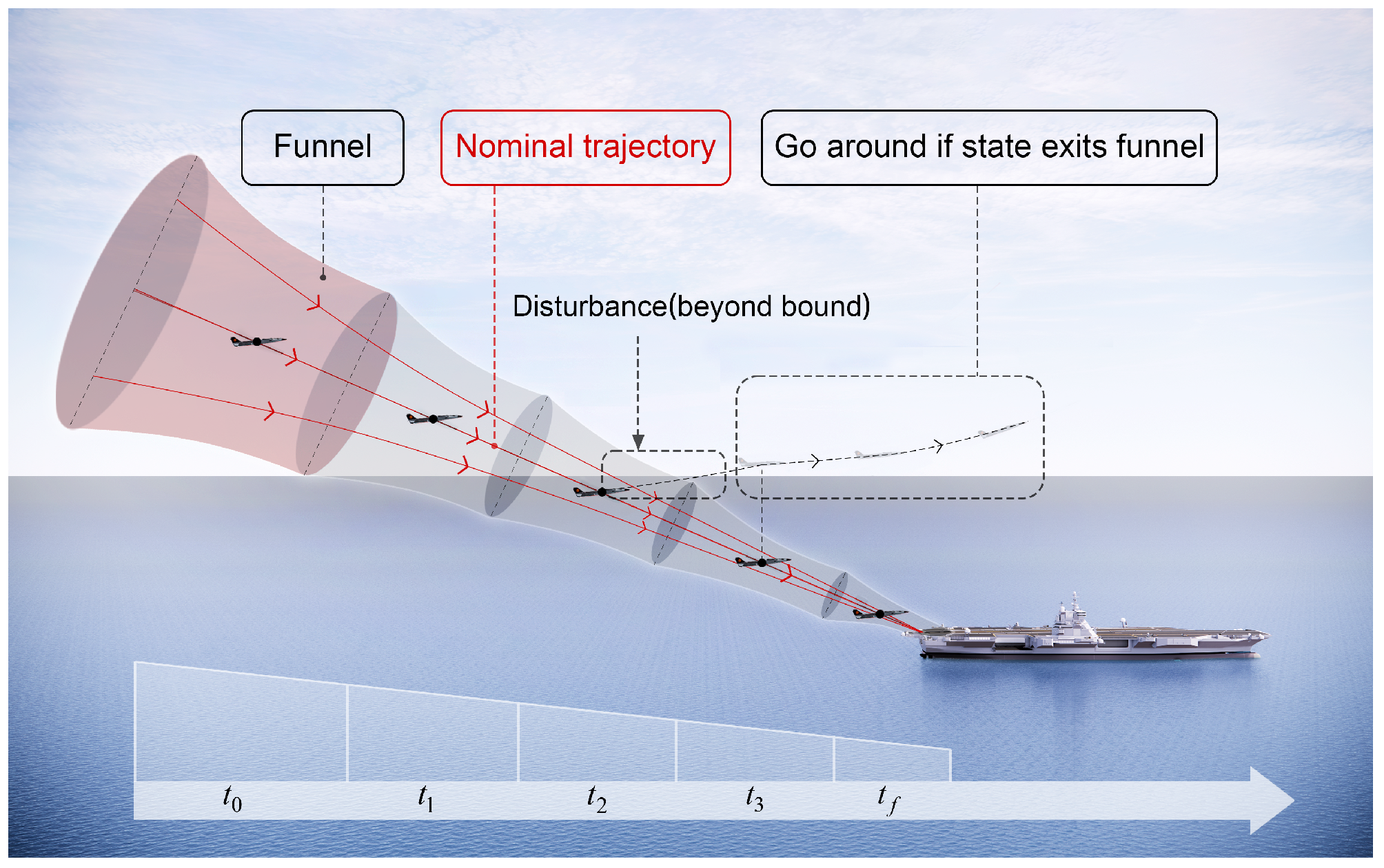
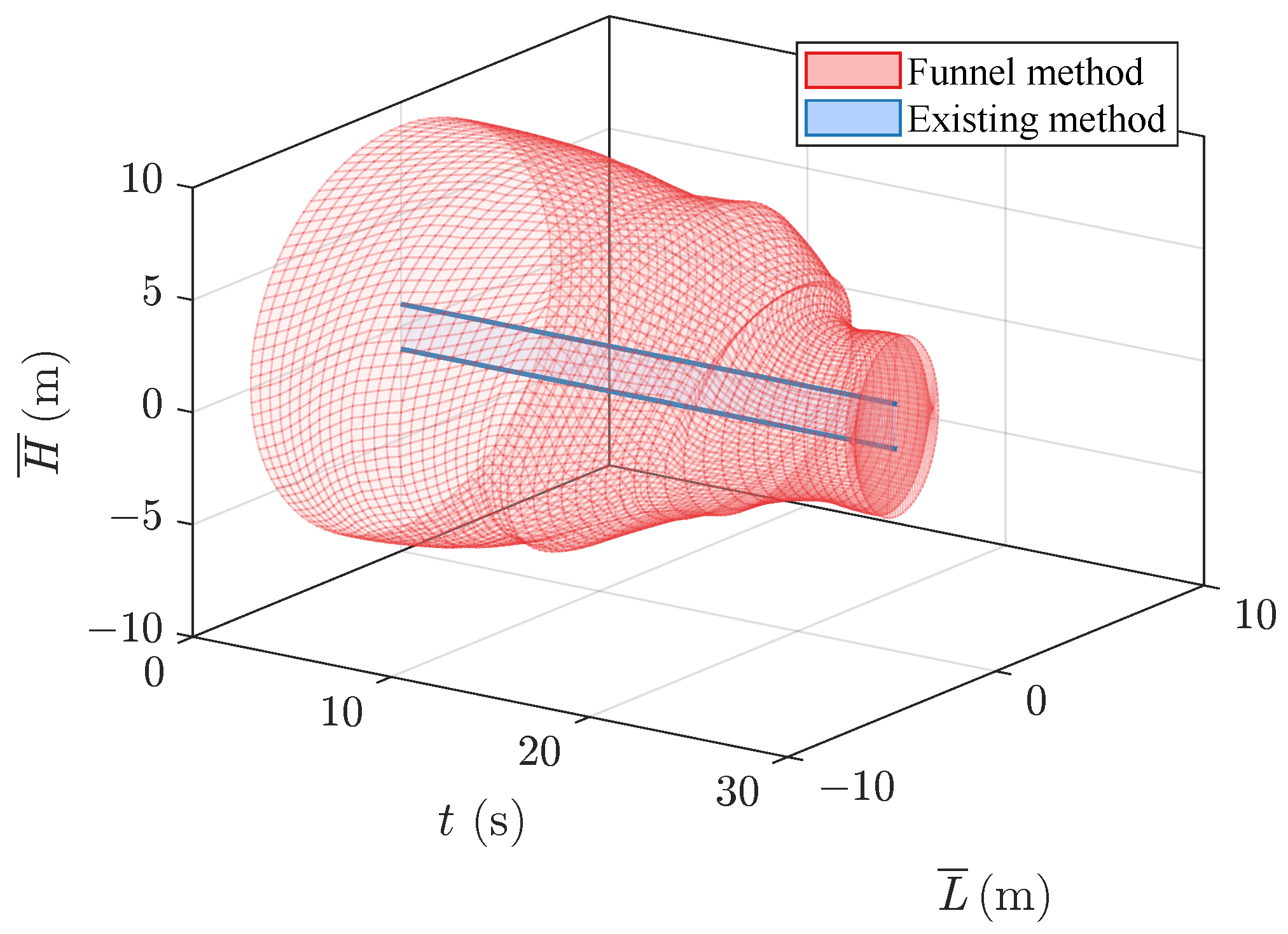
Safe and precise go-around decision-making requires an explicit characterization of the time-varying safe region in the multi-dimensional state space. To meet this requirement, this study introduces funnel theory from the field of robot motion planning, which provides a suitable means of explicitly characterizing such a region [29]. As illustrated in Figure 1, the six-dimensional funnel evolves along the nominal trajectory and explicitly characterizes the time-varying safe region in the multi-dimensional state space at each time instant. In this study, each of these safe regions is geometrically represented by a six-dimensional ellipsoid; therefore, Figure 1 provides only a schematic visualization of the six-dimensional funnel. Tedrake et al. [30] first introduced sum-of-squares (SOS) programming to address the computational challenges associated with funnel estimation. Funnel-based approaches were later successfully applied in contexts such as spacecraft rendezvous [31] and the Mars landing problem [32]. In this study, the six-dimensional funnel is constructed offline to realize the safe-region characterization defined above. Its invariance property enables it to serve as the decision boundary for online go-around decision-making. During online implementation, the online go-around decision module checks at each sampling instant whether the complete six-dimensional state deviation lies inside the precomputed funnel. If the state deviation lies inside the funnel, the module outputs the continue-landing decision; otherwise, it outputs the go-around decision.

Existing funnel-based studies have demonstrated the applicability of funnel theory to trajectory guidance problems such as powered descent [32]. However, directly applying these methods to automatic carrier-landing go-around decisions remains challenging because of the differences in the application objective and problem formulation. First, this study establishes a polynomial representation of the nonlinear longitudinal dynamics for the complete six-dimensional state, allowing the range state and the corresponding terminal requirement to be incorporated into the funnel-based go-around decision framework. Second, carrier-specific environmental effects, such as deck motion, must be incorporated into the offline computation of the corresponding decision boundary. Third, rather than using the funnel for trajectory guidance, this study uses the offline-computed six-dimensional funnel as the decision boundary for an online go-around decision rule. The online module evaluates the complete six-dimensional state deviation and outputs either the continue-landing decision or the go-around decision according to the funnel membership condition.

In summary, this study aims to establish a safety-guaranteed go-around decision framework for ACLSs by explicitly characterizing the time-varying safe region of the complete six-dimensional longitudinal state and using this region as the decision boundary for online go-around decision-making. Specifically, this study investigates how to construct such a time-varying multi-dimensional safe region while accounting for the closed-loop nonlinear dynamics, actuator saturation constraints, terminal landing requirements, and prescribed bounded uncertainties; how to use the offline-computed safe region to make online continue-landing or go-around decisions based on the complete six-dimensional state deviation; and what additional decision information and benefits can be obtained compared with the conventional single-dimensional altitude-deviation criterion. The key contributions of this study are summarized as follows:

(1)

A safety-guaranteed go-around decision framework is proposed for ACLSs. In the offline stage, a six-dimensional funnel is computed while accounting for the closed-loop polynomial dynamics, actuator saturation constraints, the terminal set reflecting the required landing precision, and prescribed bounded uncertainties. During online implementation, the offline-computed funnel serves as the decision boundary, and the online go-around decision module evaluates the complete six-dimensional state deviation to output either the continue-landing decision or the go-around decision. This framework establishes a clear separation between offline decision-boundary computation and online decision execution.

(2)

A complete six-dimensional formulation that includes the range state is developed for the carrier-landing problem. This formulation enables the range state and its corresponding terminal requirement to be incorporated into the feedback design, terminal set, and online membership test. Compared with the five-dimensional formulation, incorporating the range state reduces the mean, maximum, and standard deviation of the terminal altitude deviations by approximately 68%, 64%, and 66%, respectively, while reducing the corresponding statistics of the terminal range deviations by approximately 99%.

(3)

The effectiveness of the proposed framework is demonstrated from the perspectives of polynomial-model accuracy, representative deck-motion disturbance, conventional altitude-deviation-based decisions, and required landing precision. The second-order closed-loop polynomial system provides a more reliable offline decision boundary than the first-order approximation. Under the representative deck-motion disturbance, the framework remains effective after the six-dimensional funnel is recomputed offline, while the online decision rule remains unchanged. The proposed method also avoids unnecessary go-around decisions when the altitude deviation exceeds the conventional threshold but the complete six-dimensional state deviation remains inside the funnel, and reveals the trade-off between the required landing precision and the safe region size.

The remainder of the paper is structured as follows: Section 2 presents the nonlinear longitudinal model and the closed-loop polynomial system. Section 3 develops the offline six-dimensional funnel estimation method using SOS programming and formulates the corresponding online go-around decision rule. Section 4 evaluates the effectiveness of the proposed go-around decision framework, analyzes how polynomial-model accuracy, the inclusion of the range state, deck motion, and the required landing precision affect the offline decision boundary and the resulting online decisions, and compares the proposed complete-state decision rule with the conventional altitude-deviation-based rule. Section 5 concludes the paper and discusses future research directions.

2. Preliminaries

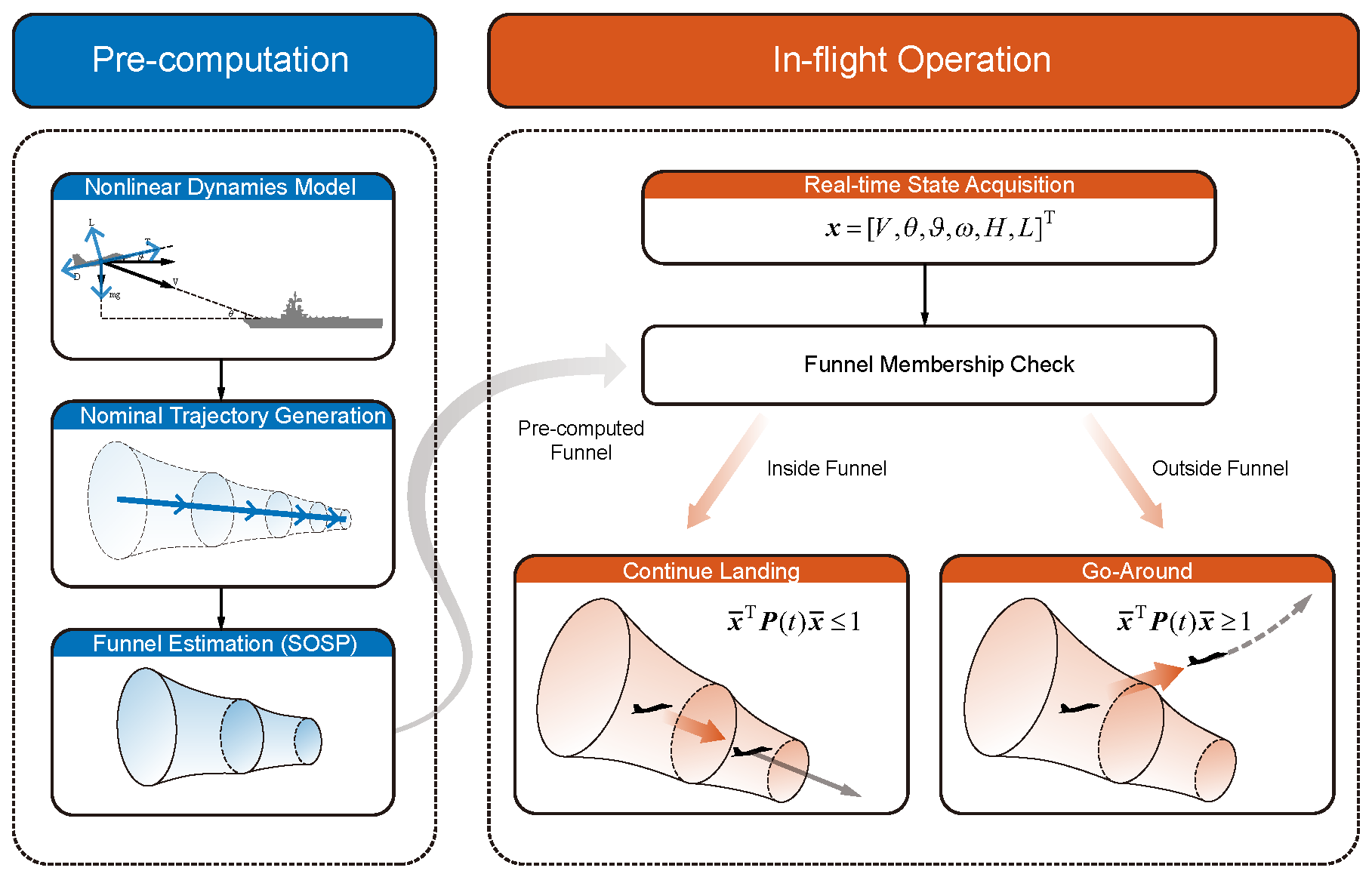
As shown in Figure 2, the safety-guaranteed go-around decision framework consists of an offline computation stage and an online implementation stage for the carrier-landing scenario illustrated in Figure 1. The “Pre-computation” block in Figure 2 corresponds to offline decision-boundary computation, whereas the “In-flight Operation” block corresponds to online decision execution. In the offline stage, the nonlinear longitudinal model is established, the nominal trajectory is generated, the corresponding closed-loop polynomial system is constructed, and the six-dimensional funnel is computed while accounting for actuator saturation constraints, the terminal set reflecting the required landing precision, and prescribed uncertainty bounds. The outputs of the offline stage are the nominal state trajectory ${\mathit{x}}_{\mathrm{op}}\left(t_k\right)$ and the precomputed funnel matrix sequence ${\left\{{\mathit{P}}_k\right\}}_{k=1}^N$, which are stored for subsequent online use. During online implementation, the current aircraft state $\mathit{x}\left(t_k\right)$ is acquired at each sampling instant. The online module retrieves the corresponding nominal state and funnel matrix, computes the complete six-dimensional state deviation as $\overline{\mathit{x}}\left(t_k\right)=\mathit{x}\left(t_k\right)-{\mathit{x}}_{\mathrm{op}}\left(t_k\right)$, and evaluates the level-set function ${\overline{\mathit{x}}}^{\top }\left(t_k\right){\mathit{P}}_k\overline{\mathit{x}}\left(t_k\right)$. The module then outputs the continue-landing decision when the complete six-dimensional state deviation lies inside the corresponding precomputed funnel and outputs the go-around decision otherwise. Therefore, the relationship between the two stages is a one-way transfer of the offline-computed nominal trajectory and funnel matrix sequence to the online decision module; no SOS optimization or funnel recomputation is performed during online implementation. In practical ACLS implementation, the proposed method can therefore be integrated as an online go-around decision module within the existing feedback-control architecture. The existing feedback controller remains responsible for tracking the nominal landing trajectory, while the proposed module independently evaluates whether the current complete six-dimensional state deviation remains within the precomputed safe region and outputs either the continue-landing decision or the go-around decision. Thus, the proposed method supplements rather than replaces the existing flight-control system.

2.1. Nonlinear Longitudinal Model

To retain the nonlinear longitudinal dynamics neglected by the small-disturbance linear models commonly adopted in conventional ACLS design, this study employs the nonlinear longitudinal model of the carrier aircraft presented in [16].

In the flight-path coordinate system, the longitudinal dynamics are expressed as follows:

$$\begin{array}{cc}\hfill \dot{V}& ={\displaystyle \frac{P_{max}{D}_{p}cos\alpha -C_{D}q{S}_{\mathrm{ref}}-mgsin\theta }{m}}\hfill \\ \hfill \dot{\theta }& ={\displaystyle \frac{P_{max}{D}_{p}sin\alpha +C_{L}q{S}_{\mathrm{ref}}-mgcos\theta }{mV}}\hfill \\ \hfill \dot{\vartheta }& =\omega \hfill \\ \hfill \dot{\omega }& ={\displaystyle \frac{C_{M}q{S}_{\mathrm{ref}}c}{I}}\hfill \\ \hfill \dot{H}& =Vsin\theta \hfill \\ \hfill \dot{L}& =Vcos\theta ,\hfill \end{array}$$

(1)

where $P_{max}$ is the maximum thrust, $D_p$ is the throttle setting, V is the airspeed, $\theta$ is the flight-path angle, $\vartheta$ is the pitch angle, $\omega$ is the pitch rate, H is the altitude, and L is the range. The angle of attack is given by $\alpha =\vartheta -\theta$, and the dynamic pressure is given by $q={\displaystyle \frac{1}{2}}\rho V^2$, where $\rho$ is the air density. In addition, g is the gravitational acceleration, m is the aircraft mass, I is the pitch moment of inertia, $S_{\mathrm{ref}}$ is the reference wing area, and c is the mean aerodynamic chord.

The nonlinear model in (1) represents the baseline longitudinal aircraft dynamics. Prescribed bounded environmental disturbances can be incorporated into the corresponding closed-loop model through the prescribed bounded uncertainty formulation introduced in Section 3.1.4. In the numerical study, the heave component of deck motion is explicitly incorporated into the altitude dynamics in Section 4.3.

The aerodynamic drag coefficient $C_D$, lift coefficient $C_L$, and pitching moment coefficient $C_M$ are given by:

$$\begin{array}{cc}\hfill C_D& =C_{D0}+C_{D\alpha }\alpha +C_{D{\alpha }^2}{\alpha }^2\hfill \\ \hfill C_L& =C_{L0}+C_{L\alpha }\alpha +C_{L{D}_z}{D}_z\hfill \\ \hfill C_M& =C_{M0}+C_{M\alpha }\alpha +C_{M{D}_z}{D}_z+C_{M\omega }\omega ,\hfill \end{array}$$

(2)

where $D_z$ is the elevator deflection.

The complete six-dimensional longitudinal state vector and the two-dimensional control vector of the nonlinear longitudinal model (1) are defined as:

$$\begin{array}{ccc}\hfill \mathit{x}& ={\left[\begin{array}{cccccc}V& \theta & \vartheta & \omega & H& L\end{array}\right]}^{\top },\mathit{u}\hfill & \hfill ={\left[\begin{array}{cc}{D}_z& D_p\end{array}\right]}^{\top }.\end{array}$$

(3)

The nonlinear longitudinal model in (1) is used to generate the nominal landing trajectory. Specifically, the nominal state trajectory ${\mathit{x}}_{\mathrm{op}}\left(t\right)$ and the corresponding nominal control trajectory ${\mathit{u}}_{\mathrm{op}}\left(t\right)$ are obtained by solving the following optimal control problem:

$$\begin{array}{cc}\hfill {\displaystyle \underset{{\mathit{x}}_{\mathrm{op}}\left(·\right),{\mathit{u}}_{\mathrm{op}}\left(·\right)\hspace{0.5em}}{min}}& J_{\mathrm{op}}={\int }_0^{t_f}{\displaystyle \frac{1}{2}}\left[D_{z,\mathrm{op}}^2\left(t\right)+D_{p,\mathrm{op}}^2\left(t\right)\right]\mathrm{d}t,\hfill \\ \hfill \mathrm{s}.\mathrm{t}.\hspace{0.5em}& {\dot{\mathit{x}}}_{\mathrm{op}}\left(t\right)=\mathit{f}\left({\mathit{x}}_{\mathrm{op}}\left(t\right),{\mathit{u}}_{\mathrm{op}}\left(t\right)\right),\hfill \\ \hfill & {\mathit{x}}_{\mathrm{op}}\left(0\right)={\mathit{x}}_0,\hfill \\ \hfill & {\mathit{x}}_{\mathrm{op}}\left(t_f\right)\in {\mathcal{X}}_{\mathrm{op},f},\hfill \\ \hfill & {\mathit{x}}_{min}\le {\mathit{x}}_{\mathrm{op}}\left(t\right)\le {\mathit{x}}_{max},\hfill \\ \hfill & {\mathit{u}}_{min}\le {\mathit{u}}_{\mathrm{op}}\left(t\right)\le {\mathit{u}}_{max},t\in [0,t_f].\hfill \end{array}$$

(4)

Here, $\mathit{f}$ denotes the right-hand side of the nonlinear dynamics in (1), and $t_f$ is the final time. The nominal state trajectory ${\mathit{x}}_{\mathrm{op}}\left(t\right)$ and nominal control trajectory ${\mathit{u}}_{\mathrm{op}}\left(t\right)$ are the decision trajectories, while ${\mathit{x}}_0$ is the prescribed initial state. The set ${\mathcal{X}}_{\mathrm{op},f}$ specifies the terminal constraints used for nominal trajectory generation and constrains the nominal terminal state ${\mathit{x}}_{\mathrm{op}}\left(t_f\right)$ in the original state space. The vectors ${\mathit{x}}_{min}$, ${\mathit{x}}_{max}$, ${\mathit{u}}_{min}$, and ${\mathit{u}}_{max}$ denote the prescribed state and control bounds, which are enforced throughout the landing process. The optimal control problem is transcribed using GPOPS-II and solved using SNOPT.

2.2. Closed-Loop Polynomial System

To enable funnel estimation by SOS programming, the dynamics are rewritten in terms of the deviation from the nominal trajectory. Specifically, the state is separated into a nominal component and a deviation component,

$$\mathit{x}\left(t\right)={\mathit{x}}_{\mathrm{op}}\left(t\right)+\overline{\mathit{x}}\left(t\right),$$

(5)

and the control input is expressed in a similar manner,

$$\mathit{u}\left(t\right)={\mathit{u}}_{\mathrm{op}}\left(t\right)+\overline{\mathit{u}}\left(t\right).$$

(6)

Here, $\mathit{x}\left(t\right)\in {\mathbb{R}}^6$ and $\mathit{u}\left(t\right)\in {\mathbb{R}}^2$ are the same state and control vectors defined in (3), respectively. Specifically, $\mathit{u}\left(t\right)={\left[D_z\left(t\right)D_p\left(t\right)\right]}^{\top }$ consists of the elevator deflection and throttle setting. The quantities ${\mathit{x}}_{\mathrm{op}}\left(t\right)\in {\mathbb{R}}^6$ and ${\mathit{u}}_{\mathrm{op}}\left(t\right)\in {\mathbb{R}}^2$ denote the nominal state and control trajectories obtained through offline trajectory planning, while $\overline{\mathit{x}}\left(t\right)\in {\mathbb{R}}^6$ and $\overline{\mathit{u}}\left(t\right)\in {\mathbb{R}}^2$ denote the corresponding deviations from the nominal trajectories.

The nonlinear longitudinal model is first linearized along the nominal trajectory. Substituting (5) and (6) into the nonlinear longitudinal model and retaining the first-order terms yields the following linear time-varying deviation model:

$$\begin{array}{cc}\hfill \dot{\overline{\mathit{x}}}\left(t\right)& =\mathit{A}\left(t\right)\overline{\mathit{x}}\left(t\right)+\mathit{B}\left(t\right)\overline{\mathit{u}}\left(t\right).\hfill \end{array}$$

(7)

The state and control matrices are obtained by linearizing the nonlinear longitudinal model around the nominal state and control trajectories:

$$\begin{array}{cc}\hfill \mathit{A}\left(t\right)& ={\left.{\displaystyle \frac{\partial \mathit{f}(\mathit{x},\mathit{u})}{\partial \mathit{x}}}\right|}_{\mathit{x}={\mathit{x}}_{\mathrm{op}}\left(t\right),\mathit{u}={\mathit{u}}_{\mathrm{op}}\left(t\right)},\hfill \\ \hfill \mathit{B}\left(t\right)& ={\left.{\displaystyle \frac{\partial \mathit{f}(\mathit{x},\mathit{u})}{\partial \mathit{u}}}\right|}_{\mathit{x}={\mathit{x}}_{\mathrm{op}}\left(t\right),\mathit{u}={\mathit{u}}_{\mathrm{op}}\left(t\right)}.\hfill \end{array}$$

(8)

Here, $\mathit{A}\left(t\right)\in {\mathbb{R}}^{6\times 6}$ and $\mathit{B}\left(t\right)\in {\mathbb{R}}^{6\times 2}$. Since the nominal state and control trajectories vary throughout the landing process, the nonlinear longitudinal model is linearized along the entire nominal trajectory rather than at a single fixed operating point. In the numerical implementation, $\mathit{A}\left(t_k\right)$ and $\mathit{B}\left(t_k\right)$ are evaluated at each discretization point $t_k$ using the corresponding nominal state ${\mathit{x}}_{\mathrm{op}}\left(t_k\right)$, nominal control ${\mathit{u}}_{\mathrm{op}}\left(t_k\right)$, the nonlinear dynamics in (1), and the aircraft parameters listed in

Table 1. Parameters of carrier-based aircraft.

Parameter	Value
Mass m	16,374 $\mathrm{k}\mathrm{g}$
Pitch moment of inertia I	239,720 $\mathrm{k}\mathrm{g}$·${\mathrm{m}}^2$
Reference wing area $S_{\mathrm{ref}}$	$37.16$ m2
Mean aerodynamic chord c	$3.51$ m
Drag coefficient $C_{D0}$	0.1423
Lift coefficient $C_{L0}$	0.732
Drag coefficient $C_{D\alpha }$	$-0.00438$
Lift coefficient $C_{L\alpha }$	0.0751
Drag coefficient $C_{D{\alpha }^2}$	0.0013
Lift coefficient $C_{L{D}_z}$	0.0144
Moment coefficient $C_{M0}$	$-0.1885$
Moment coefficient $C_{M\alpha }$	$-0.00437$
Moment coefficient $C_{M{D}_z}$	$-0.0196$
Moment coefficient $C_{M\omega }$	$-0.123$

. The linear time-varying deviation model in (7) is used to design the LQR controller. The subsequent funnel estimation is performed using a polynomial approximation of the resulting closed-loop nonlinear error dynamics.

The linear-quadratic regulator (LQR) is employed to obtain the deviation feedback control law $\overline{\mathit{u}}\left(t\right)$. Given the weighting matrices ${\mathit{Q}}_f$, $\mathit{Q}\left(t\right)$, and $\mathit{R}\left(t\right)$, the corresponding Riccati differential equation is

$$\begin{array}{cc}\hfill \dot{\mathit{S}}\left(t\right)& =-\mathit{Q}\left(t\right)-\mathit{A}{\left(t\right)}^{\top }\mathit{S}\left(t\right)-\mathit{S}\left(t\right)\mathit{A}\left(t\right)\hfill \\ \hfill & +\mathit{S}\left(t\right)\mathit{B}\left(t\right)\mathit{R}{\left(t\right)}^{-1}\mathit{B}{\left(t\right)}^{\top }\mathit{S}\left(t\right),\hfill \\ \hfill \mathit{S}\left(t_f\right)& ={\mathit{Q}}_f.\hfill \end{array}$$

(9)

Solving (9) yields the positive-definite Riccati matrix $\mathit{S}\left(t\right)$. The resulting time-varying LQR feedback gain and deviation feedback control law are given by

$$\begin{array}{cc}\hfill \overline{\mathit{u}}\left(t\right)& =-\mathit{K}\left(t\right)\overline{\mathit{x}}\left(t\right),\hfill \\ \hfill \mathit{K}\left(t\right)& \triangleq \mathit{R}{\left(t\right)}^{-1}\mathit{B}{\left(t\right)}^{\top }\mathit{S}\left(t\right).\hfill \end{array}$$

(10)

After substituting the closed-loop control law $\mathit{u}\left(t\right)={\mathit{u}}_{\mathrm{op}}\left(t\right)-\mathit{K}\left(t\right)\overline{\mathit{x}}\left(t\right)$ into the nonlinear longitudinal model (1), the exact closed-loop error dynamics are expressed as

$$\begin{array}{cc}\hfill \dot{\overline{\mathit{x}}}\left(t\right)& ={\mathit{f}}_{\mathrm{cl}}\left(\overline{\mathit{x}}\left(t\right),t\right)\hfill \\ \hfill & \triangleq \mathit{f}\left({\mathit{x}}_{\mathrm{op}}\left(t\right)+\overline{\mathit{x}}\left(t\right),{\mathit{u}}_{\mathrm{op}}\left(t\right)-\mathit{K}\left(t\right)\overline{\mathit{x}}\left(t\right)\right)\hfill \\ \hfill & -\mathit{f}\left({\mathit{x}}_{\mathrm{op}}\left(t\right),{\mathit{u}}_{\mathrm{op}}\left(t\right)\right).\hfill \end{array}$$

(11)

For subsequent funnel estimation via SOS programming, the exact closed-loop error dynamics in (11) are approximated by a polynomial in the state deviation at each time instant along the nominal trajectory. Specifically, a Taylor expansion about $\overline{\mathit{x}}=0$ is performed with the selected truncation order, yielding the closed-loop polynomial system

$$\dot{\overline{\mathit{x}}}\left(t\right)\approx \mathit{p}\left(\overline{\mathit{x}}\left(t\right),t\right).$$

(12)

Based on the closed-loop polynomial system in (12), the funnel estimation problem can be formulated using sum-of-squares programming. Specifically, the polynomial nonnegativity conditions associated with funnel invariance and the actuator saturation constraints are converted into SOS constraints, which are subsequently represented as semidefinite programming subproblems. Since the resulting formulation contains bilinear terms between the funnel variables and SOS multipliers, it is solved using the backward point-by-point alternating strategy detailed in Section 3.

3. Offline Funnel Computation and Online Go-Around Decision Rule

This section establishes the mathematical basis of the proposed go-around decision framework through three parts. First, the six-dimensional funnel is formulated offline as a time-varying safe region for the closed-loop polynomial system using SOS programming [30]. The terminal-set inclusion, invariance, actuator saturation, and prescribed bounded uncertainty conditions give the funnel membership condition a direct decision meaning: a complete six-dimensional state deviation inside the corresponding funnel is associated with a closed-loop trajectory that remains within the subsequent funnel, satisfies the actuator saturation constraints, and reaches the terminal set under the prescribed uncertainty bounds. Second, a backward point-by-point computation strategy is employed to obtain the funnel sequence and the corresponding time-varying decision boundary efficiently [32]. Third, during online implementation, the current complete six-dimensional state deviation is evaluated against the corresponding precomputed funnel at each sampling instant, and the online go-around decision module outputs either the continue-landing decision or the go-around decision.

3.1. Offline Backward Funnel Formulation

The six-dimensional funnel used as the online decision boundary is defined along the nominal trajectory over the interval $[0,t_f]$ as a time-varying ellipsoidal set in ${\mathbb{R}}^n$:

$$F\left(t\right)=\left\{\overline{\mathit{x}}|V(\overline{\mathit{x}},t)\triangleq {\overline{\mathit{x}}}^{\top }\mathit{P}\left(t\right)\overline{\mathit{x}}\le 1\right\}.$$

(13)

Here, $V(\overline{\mathit{x}},t)$ is the level-set function, and $\mathit{P}\left(t\right)$ is a symmetric positive-definite matrix that determines the shape of the funnel ellipsoid. For the complete six-dimensional longitudinal state considered in this study, $n=6$ and $\mathit{P}\left(t\right)\in {\mathbb{S}}_{++}^6$. To enable numerical computation, the time interval $[0,t_f]$ is discretized into N time points $t_k$ $(k=1,\dots ,N)$, where $t_1=0$ and $t_N=t_f$. At each discrete time point, the corresponding six-dimensional funnel is represented as

$$F\left(t_k\right)=\left\{\overline{\mathit{x}}|V_k\left(\overline{\mathit{x}}\right)\triangleq {\overline{\mathit{x}}}^{\top }{\mathit{P}}_k\overline{\mathit{x}}\le 1\right\}.$$

(14)

Accordingly, the offline funnel computation determines the sequence of shape matrices ${\left\{{\mathit{P}}_k\right\}}_{k=1}^N$ subject to the terminal-set inclusion condition, funnel invariance condition, actuator saturation constraints, and prescribed bounded uncertainty constraints introduced below. These conditions ensure that the resulting funnel sequence provides a valid time-varying safe region and decision boundary for the subsequent online membership test.

3.1.1. Funnel Terminal-Set Inclusion Condition

To ensure that the online continue-landing decision is consistent with the required landing precision, the terminal set is specified as the following ellipsoid:

$${\mathcal{X}}_f=\left\{\overline{\mathit{x}}|{\overline{\mathit{x}}}^{\top }\mathit{E}\overline{\mathit{x}}\le 1\right\}.$$

(15)

Here, $\mathit{E}\in {\mathbb{S}}_{++}^6$ is the shape matrix of the terminal ellipsoid. The terminal set encodes the required landing precision together with any additional terminal-state requirements prescribed for the considered formulation. In the six-dimensional formulation examined in this study, the range state and its corresponding terminal requirement are additionally incorporated into the terminal set. To ensure that the terminal funnel is contained within ${\mathcal{X}}_f$, the following inclusion condition is imposed:

$${\mathit{P}}_N-\mathit{E}⪰\mathbf{0}.$$

(16)

This condition guarantees that $F\left(t_f\right)\subseteq {\mathcal{X}}_f$ and therefore ensures that the offline decision boundary is consistent with the required landing precision at the final time. The funnel invariance condition introduced next establishes the connection between current funnel membership and eventual arrival at this terminal set.

3.1.2. Funnel Invariance Condition

To ensure that the funnel membership condition provides a valid basis for the online go-around decision, an invariance condition is imposed on the funnel boundary. Specifically, a complete six-dimensional state deviation classified as lying inside the funnel at time $t_k$ must be associated with a closed-loop trajectory that remains within the subsequent funnel. Therefore, the online membership test reflects the predicted evolution of the closed-loop trajectory over the landing process rather than only an instantaneous geometric relation. This requirement is enforced through the following boundary implication:

$$V_k\left(\overline{\mathit{x}}\right)=1\Rightarrow -{\dot{V}}_k\left(\overline{\mathit{x}}\right)\ge 0,k=1,\dots ,N-1.$$

(17)

The derivative of the level-set function at $t_k$ is approximated as

$$\begin{array}{cc}\hfill {\dot{V}}_k\left(\overline{\mathit{x}}\right)& =2{\overline{\mathit{x}}}^{\top }{\mathit{P}}_k\dot{\overline{\mathit{x}}}+{\overline{\mathit{x}}}^{\top }{\dot{\mathit{P}}}_k\overline{\mathit{x}}\hfill \\ & \approx 2{\overline{\mathit{x}}}^{\top }{\mathit{P}}_k\mathit{p}\left(\overline{\mathit{x}},t_k\right)+{\displaystyle \frac{V_{k+1}\left(\overline{\mathit{x}}\right)-V_k\left(\overline{\mathit{x}}\right)}{t_{k+1}-t_k}}.\hfill \end{array}$$

(18)

Using the S-procedure, the implication in (17) is imposed through the following SOS constraint:

$$-{\dot{V}}_k\left(\overline{\mathit{x}}\right)-L_k\left(\overline{\mathit{x}}\right)\left(1-V_k\left(\overline{\mathit{x}}\right)\right)\mathrm{is}\mathrm{SOS}.$$

(19)

Here, $L_k\left(\overline{\mathit{x}}\right)$ is a multiplier polynomial. Together with the funnel terminal-set inclusion condition, the invariance condition gives the online membership test a predictive and terminal meaning for the deterministic closed-loop polynomial system. Specifically, if the current complete six-dimensional state deviation lies inside the corresponding funnel, the associated closed-loop trajectory is required to remain within the subsequent funnel and eventually enter the terminal set. Therefore, the continue-landing decision is based on the predicted closed-loop evolution over the landing process rather than on a single instantaneous state threshold. The extension of this condition to prescribed bounded uncertainties is introduced in Section 3.1.4.

3.1.3. Actuator Saturation Constraints

To ensure that a continue-landing decision based on funnel membership is compatible with the physical control capabilities of the carrier aircraft, the elevator deflection and throttle setting must satisfy their actuator saturation constraints. For the jth control component, these constraints are expressed as

$$u_{min,j}\le u_j\left(t\right)\le u_{max,j},j=1,2.$$

(20)

At the discrete time point $t_k$, the corresponding closed-loop control input is given by

$$u_{j,k}\left(\overline{\mathit{x}}\right)\triangleq u_{\mathrm{op},j}\left(t_k\right)-{\mathit{K}}_j\left(t_k\right)\overline{\mathit{x}},$$

(21)

where ${\mathit{K}}_j\left(t_k\right)$ denotes the jth row of the feedback gain matrix $\mathit{K}\left(t_k\right)$. To ensure that every complete six-dimensional state deviation inside the funnel is associated with admissible control inputs, the following implication is imposed for $j=1,2$ and $k=1,\dots ,N-1$:

$$V_k\left(\overline{\mathit{x}}\right)\le 1\Rightarrow \left\{\begin{array}{c}{u}_{j,k}\left(\overline{\mathit{x}}\right)-u_{min,j}\ge 0,\hfill \\ u_{max,j}-u_{j,k}\left(\overline{\mathit{x}}\right)\ge 0.\hfill \end{array}\right.$$

(22)

Using the S-procedure, the lower-bound constraint is formulated as

$$u_{j,k}\left(\overline{\mathit{x}}\right)-u_{min,j}-L_{Lj,k}\left(\overline{\mathit{x}}\right)\left(1-V_k\left(\overline{\mathit{x}}\right)\right)\mathrm{is}\mathrm{SOS},$$

(23)

$$L_{Lj,k}\left(\overline{\mathit{x}}\right)\mathrm{is}\mathrm{SOS},$$

(24)

and the upper-bound constraint is formulated as

$$u_{max,j}-u_{j,k}\left(\overline{\mathit{x}}\right)-L_{Uj,k}\left(\overline{\mathit{x}}\right)\left(1-V_k\left(\overline{\mathit{x}}\right)\right)\mathrm{is}\mathrm{SOS},$$

(25)

$$L_{Uj,k}\left(\overline{\mathit{x}}\right)\mathrm{is}\mathrm{SOS},$$

(26)

where $L_{Lj,k}\left(\overline{\mathit{x}}\right)$ and $L_{Uj,k}\left(\overline{\mathit{x}}\right)$ are SOS multiplier polynomials for $j=1,2$ and $k=1,\dots ,N-1$. These constraints are imposed separately on the elevator deflection and throttle setting at each discrete time point. Together with the funnel invariance condition, they ensure that a complete six-dimensional state deviation classified as lying inside the funnel is associated with closed-loop control inputs that remain within the prescribed actuator limits throughout the landing process. Therefore, the continue-landing decision is supported not only by terminal reachability but also by the physical feasibility of the required control inputs.

3.1.4. Prescribed Bounded Uncertainty Constraints

To ensure that the offline-computed decision boundary remains valid under the prescribed bounded effects, a bounded uncertainty variable is incorporated into the closed-loop polynomial system. Environmental disturbances, modeling errors, and Taylor truncation errors can be accommodated through this unified representation when their corresponding bounds are prescribed [32]. Accordingly, the closed-loop polynomial system in (12) is extended as

$$\dot{\overline{\mathit{x}}}\left(t\right)\approx \mathit{p}\left(\overline{\mathit{x}}\left(t\right),t,\mathit{w}\right),\mathit{w}\in \mathcal{W},$$

(27)

where $\mathit{w}$ denotes the bounded term introduced for the considered uncertainty, and $\mathcal{W}$ denotes the corresponding prescribed bounded set. For different bounded effects, $\mathit{w}$ and $\mathcal{W}$ are specified accordingly. The bounded set is described by polynomial inequalities as

$$\mathcal{W}=\left\{\mathit{w}|g_i\left(\mathit{w}\right)\ge 0,i=1,\dots ,n_w\right\},$$

(28)

where $g_i\left(\mathit{w}\right)$ is the polynomial function defining the ith bound, and $n_w$ is the number of polynomial inequalities used to describe $\mathcal{W}$.

To ensure that the funnel invariance condition holds for all bounded effects contained in $\mathcal{W}$, the boundary implication in (17) is extended as

$$V_k\left(\overline{\mathit{x}}\right)=1,\mathit{w}\in \mathcal{W}\Rightarrow -{\dot{V}}_k(\overline{\mathit{x}},\mathit{w})\ge 0,$$

(29)

for $k=1,\dots ,N-1$. Under the prescribed bounded uncertainty, the derivative of the level-set function is approximated as

$$\begin{array}{cc}\hfill {\dot{V}}_k(\overline{\mathit{x}},\mathit{w})& =2{\overline{\mathit{x}}}^{\top }{\mathit{P}}_k\dot{\overline{\mathit{x}}}+{\overline{\mathit{x}}}^{\top }{\dot{\mathit{P}}}_k\overline{\mathit{x}}\hfill \\ & \approx 2{\overline{\mathit{x}}}^{\top }{\mathit{P}}_k\mathit{p}\left(\overline{\mathit{x}},t_k,\mathit{w}\right)\hfill \\ \hfill & +{\displaystyle \frac{V_{k+1}\left(\overline{\mathit{x}}\right)-V_k\left(\overline{\mathit{x}}\right)}{t_{k+1}-t_k}}.\hfill \end{array}$$

(30)

Using the S-procedure, the implication in (29) is imposed through the following SOS constraint:

$$\begin{array}{cc}\hfill & -{\dot{V}}_k(\overline{\mathit{x}},\mathit{w})-L_k(\overline{\mathit{x}},\mathit{w})\left(1-V_k\left(\overline{\mathit{x}}\right)\right)\hfill \\ \hfill & -{\displaystyle \sum _{i=1}^{n_w}}{L}_{Wi,k}(\overline{\mathit{x}},\mathit{w})g_i\left(\mathit{w}\right)\mathrm{is}\mathrm{SOS}.\hfill \end{array}$$

(31)

Here, $L_k(\overline{\mathit{x}},\mathit{w})$ is a polynomial multiplier associated with the funnel boundary condition. The multiplier polynomials associated with the prescribed bounded set satisfy

$$L_{Wi,k}(\overline{\mathit{x}},\mathit{w})\mathrm{is}\mathrm{SOS},i=1,\dots ,n_w.$$

(32)

For the funnel computation under prescribed bounded uncertainties, the robust SOS constraint in (31) is used in place of the deterministic invariance constraint in (19). It requires the funnel invariance condition to hold for every bounded effect contained in $\mathcal{W}$. When no uncertainty is considered, the robust formulation reduces to the deterministic invariance condition. In the numerical study, the heave component of deck motion is treated as a representative bounded environmental disturbance, and its effect is incorporated into the longitudinal dynamics before the corresponding closed-loop polynomial system and funnel are recomputed offline. Other bounded environmental effects, such as atmospheric disturbances, can be incorporated through the same formulation when their corresponding models and admissible bounds are specified.

Together with the funnel terminal-set inclusion condition and actuator saturation constraints, the prescribed bounded uncertainty condition ensures that a complete six-dimensional state deviation inside the corresponding funnel is associated with a closed-loop trajectory that remains within the subsequent funnel, satisfies the actuator saturation constraints, and reaches the terminal set under the prescribed uncertainty bounds. The prescribed bounded set affects the shape matrices ${\mathit{P}}_k$ computed offline and hence the resulting time-varying decision boundary, but it does not change the go-around decision rule. If the actual uncertainty exceeds the prescribed bounds, this guarantee is no longer established. If the resulting complete six-dimensional state deviation leaves the funnel, the online go-around decision module detects the membership violation and outputs the go-around decision.

3.1.5. Offline Decision-Boundary Optimization Formulation

To reduce conservatism in online go-around decision-making, the offline computation seeks to enlarge the six-dimensional funnel while satisfying the terminal-set inclusion condition, funnel invariance condition, actuator saturation constraints, and prescribed bounded uncertainty constraints. Since the funnel defines the continue-landing decision region and its boundary separates the continue-landing and go-around decisions, enlarging the funnel increases the range of complete six-dimensional state deviations for which the continue-landing decision can be supported by the offline-computed conditions.

The volume of the funnel ellipsoid at $t_k$, up to a dimension-dependent constant, is proportional to (${\det {\mathit{P}}_k)}^{-1/2}$ [33]. Directly minimizing $logdet\left({\mathit{P}}_k\right)$ is nonconvex. Therefore, a fixed positive-definite scaling matrix ${\mathit{M}}_k$ and a positive scalar ${\sigma }_k$ are introduced through the following constraint:

$${\sigma }_k{\mathit{M}}_k⪰{\mathit{P}}_k,k=1,\dots ,N-1.$$

(33)

This condition guarantees that the ellipsoid defined by ${\sigma }_k{\mathit{M}}_k$ is contained within the funnel $F\left(t_k\right)$. For a fixed ${\mathit{M}}_k$, minimizing ${\sigma }_k$ enlarges this inner ellipsoid and therefore promotes enlargement of the corresponding funnel and its continue-landing decision region. In this study, ${\mathit{M}}_k$ is chosen as the identity matrix ${\mathit{I}}_n$ and remains fixed during the optimization, where $n=6$ for the complete six-dimensional formulation.

For the backward computation, the terminal shape matrix is fixed as ${\mathit{P}}_N=\mathit{E}$, which satisfies the terminal-set inclusion condition in (16) with equality. Based on the preceding conditions, the overall offline decision-boundary computation problem is formulated as follows:

P1

$$

given 

${\mathit{P}}_N=\mathit{E}$ and ${\mathit{M}}_k={\mathit{I}}_n$ $(k=1,\dots ,N-1)$

find  

${\mathit{P}}_k,{\sigma }_k,L_k(\overline{\mathit{x}},\mathit{w})$ $(k=1,\dots ,N-1)$

$L_{Wi,k}(\overline{\mathit{x}},\mathit{w})$ $(i=1,\dots ,n_w;k=1,\dots ,N-1)$

$L_{Lj,k}\left(\overline{\mathit{x}}\right),L_{Uj,k}\left(\overline{\mathit{x}}\right)$ $(j=1,2;k=1,\dots ,N-1)$

min  

${\displaystyle {\displaystyle \sum _{k=1}^{N-1}}{\sigma }_k}$

s.t.   

${\mathit{P}}_k\in {\mathbb{S}}_{++}^n,{\sigma }_k>0$ $(k=1,\dots ,N-1)$

(31), (32), (23), (24), (25), (26), and (33).

The solution of P1 determines the sequence of shape matrices ${\left\{{\mathit{P}}_k\right\}}_{k=1}^N$, with ${\mathit{P}}_N=\mathit{E}$, that defines the offline six-dimensional funnel and its time-varying decision boundary. This precomputed matrix sequence is subsequently used by the online go-around decision module without solving the SOS optimization problem during online operation.

3.2. Backward Point-by-Point Decision-Boundary Computation

Solving P1 for all shape matrices ${\mathit{P}}_k$ simultaneously introduces a large number of decision variables and constraints, makes the design of feasible initial guesses difficult, and leads to low computational efficiency. Therefore, a backward point-by-point computation strategy is adopted [32]. Because the terminal shape matrix is fixed as ${\mathit{P}}_N=\mathit{E}$, the remaining $N-1$ shape matrices can be computed successively for $k=N-1,N-2,\dots ,1$. At each time point, ${\mathit{P}}_{k+1}$ is treated as known, and the following local problem is solved:

P1(k)

$$

given 

${\mathit{P}}_{k+1}$ and ${\mathit{M}}_k={\mathit{I}}_n$

find  

${\mathit{P}}_k,{\sigma }_k,L_k(\overline{\mathit{x}},\mathit{w})$

$L_{Wi,k}(\overline{\mathit{x}},\mathit{w})$ $(i=1,\dots ,n_w)$

$L_{Lj,k}\left(\overline{\mathit{x}}\right),L_{Uj,k}\left(\overline{\mathit{x}}\right)$ $(j=1,2)$

min  

${\sigma }_k$

s.t.   

${\mathit{P}}_k\in {\mathbb{S}}_{++}^n,{\sigma }_k>0$

(31), (32), (23), (24), (25), (26), and (33).

Problem P1(k) contains bilinear terms between the shape matrix and multiplier polynomials, such as $L_k(\overline{\mathit{x}},\mathit{w})V_k\left(\overline{\mathit{x}}\right)$. Therefore, the shape matrix and multiplier polynomials cannot be optimized simultaneously within a standard SOS program. Following the bilinear alternating-search strategy in [31], the multiplier polynomials are first optimized for a fixed candidate ${\mathit{P}}_k$, after which ${\mathit{P}}_k$ is updated with the multipliers fixed.

For a fixed candidate ${\mathit{P}}_k$, the invariance multiplier subproblem is formulated as $\mathrm{P}1{\left(k\right)}_L^I$

given 

${\mathit{P}}_{k+1}$ and ${\mathit{P}}_k$

find  

$L_k(\overline{\mathit{x}},\mathit{w}),L_{Wi,k}(\overline{\mathit{x}},\mathit{w})$ $(i=1,\dots ,n_w)$, and ${\gamma }_I$

max  

${\gamma }_I$

s.t.   

$-{\dot{V}}_k(\overline{\mathit{x}},\mathit{w})-L_k(\overline{\mathit{x}},\mathit{w})\left(1-V_k\left(\overline{\mathit{x}}\right)\right)$

${\displaystyle -{\displaystyle \sum _{i=1}^{n_w}}{L}_{Wi,k}(\overline{\mathit{x}},\mathit{w})g_i\left(\mathit{w}\right)-{\gamma }_I\mathrm{is}\mathrm{SOS}}$

$L_{Wi,k}(\overline{\mathit{x}},\mathit{w})\mathrm{is}\mathrm{SOS}$ $(i=1,\dots ,n_w)$.

For the lower actuator bound of the jth control component, the corresponding multiplier subproblem is

$\mathrm{P}1{\left(k\right)}_L^{Lj}$

$$

given 

${\mathit{P}}_k$

find  

$L_{Lj,k}\left(\overline{\mathit{x}}\right)$ and ${\gamma }_{Lj}$

max  

${\gamma }_{Lj}$

s.t.    

$u_{j,k}\left(\overline{\mathit{x}}\right)-u_{min,j}-L_{Lj,k}\left(\overline{\mathit{x}}\right)\left(1-V_k\left(\overline{\mathit{x}}\right)\right)-{\gamma }_{Lj}\mathrm{is}\mathrm{SOS}$

$L_{Lj,k}\left(\overline{\mathit{x}}\right)\mathrm{is}\mathrm{SOS}$,      $j=1,2$.

For the upper actuator bound of the jth control component, the corresponding multiplier subproblem is

$\mathrm{P}1{\left(k\right)}_L^{Uj}$

$$

given 

${\mathit{P}}_k$

find  

$L_{Uj,k}\left(\overline{\mathit{x}}\right)$ and ${\gamma }_{Uj}$

max  

${\gamma }_{Uj}$

s.t.    

$u_{max,j}-u_{j,k}\left(\overline{\mathit{x}}\right)-L_{Uj,k}\left(\overline{\mathit{x}}\right)\left(1-V_k\left(\overline{\mathit{x}}\right)\right)-{\gamma }_{Uj}\mathrm{is}\mathrm{SOS}$

$L_{Uj,k}\left(\overline{\mathit{x}}\right)\mathrm{is}\mathrm{SOS}$,      $j=1,2$.

The three types of multiplier subproblems are collectively denoted by $\mathrm{P}1{\left(k\right)}_L$ and can be solved independently. A candidate ${\mathit{P}}_k$ is feasible if ${\gamma }_I\ge 0$, ${\gamma }_{Lj}\ge 0$, and ${\gamma }_{Uj}\ge 0$ for both control components.

With all multiplier polynomials fixed, the shape-matrix update subproblem is formulated as

$\mathrm{P}1{\left(k\right)}_P$

$$

given 

${\mathit{P}}_{k+1}$, $L_k(\overline{\mathit{x}},\mathit{w})$, $L_{Wi,k}(\overline{\mathit{x}},\mathit{w})$ $(i=1,\dots ,n_w)$,

$L_{Lj,k}\left(\overline{\mathit{x}}\right)$ and $L_{Uj,k}\left(\overline{\mathit{x}}\right)$ $(j=1,2)$

find  

${\mathit{P}}_k^{\mathrm{new}}$ and ${\sigma }_k$

min  

${\sigma }_k$

s.t.   

${\mathit{P}}_k^{\mathrm{new}}\in {\mathbb{S}}_{++}^n,{\sigma }_k>0$

(31), (23), (25), and (33).

In $\mathrm{P}1{\left(k\right)}_P$, the occurrences of ${\mathit{P}}_k$ in the listed constraints are replaced by the new decision variable ${\mathit{P}}_k^{\mathrm{new}}$. The iterative procedure used to solve P1(k) is summarized in Algorithm 1.

Algorithm 1 Backward bilinear search for P1(k)

Step0     Initialize the point-by-point computation Set the convergence tolerance $\epsilon >0$, choose the initial candidate ${\mathit{P}}_k={\mathit{P}}_{k+1}$, and specify a roll-back factor $b>1$.

Step1     Obtain a feasible shape matrix Substitute ${\mathit{P}}_{k+1}$ and the current ${\mathit{P}}_k$ into $\mathrm{P}1{\left(k\right)}_L^I$, $\mathrm{P}1{\left(k\right)}_L^{Lj}$, and $\mathrm{P}1{\left(k\right)}_L^{Uj}$ and solve the multiplier subproblems. If ${\gamma }_I\ge 0$, ${\gamma }_{Lj}\ge 0$, and ${\gamma }_{Uj}\ge 0$ for $j=1,2$, the current ${\mathit{P}}_k$ is feasible and the algorithm proceeds to Step2. Otherwise, update ${\mathit{P}}_k=b{\mathit{P}}_k$ and repeat Step1.

Step2     Refine the shape matrix Substitute ${\mathit{P}}_{k+1}$ and the multiplier polynomials obtained in Step1 into $\mathrm{P}1{\left(k\right)}_P$ to obtain ${\mathit{P}}_k^{\mathrm{new}}$.

Step3     Check convergence Compute the ellipsoid volumes before and after Step2, up to the common dimension-dependent constant, using $\mathrm{vol}={\left(\det \mathit{P}\right)}^{-1/2}$. If $({\mathrm{vol}}^{\mathrm{new}}-{\mathrm{vol}}^{\mathrm{pre}})/\left|{\mathrm{vol}}^{\mathrm{pre}}\right|\le \epsilon$, set ${\mathit{P}}_k={\mathit{P}}_k^{\mathrm{new}}$ and terminate the computation of P1(k). Otherwise, proceed to Step4.

Step4     Update the multiplier polynomials Set ${\mathit{P}}_k={\mathit{P}}_k^{\mathrm{new}}$, reinsert ${\mathit{P}}_{k+1}$ and ${\mathit{P}}_k$ into the multiplier subproblems, and return to Step2.

Starting from ${\mathit{P}}_N=\mathit{E}$ and applying this procedure for $k=N-1,N-2,\dots ,1$ yields the complete matrix sequence ${\left\{{\mathit{P}}_k\right\}}_{k=1}^N$. The entire SOS computation is performed offline. The resulting sequence defines the time-varying six-dimensional decision boundary subsequently used by the online go-around decision module.

3.3. Online Go-Around Decision Rule

During online implementation, no SOS problem is solved and the funnel is not recomputed. At each sampling instant $t_k$, the current complete six-dimensional state deviation is calculated as

$$\overline{\mathit{x}}\left(t_k\right)=\mathit{x}\left(t_k\right)-{\mathit{x}}_{\mathrm{op}}\left(t_k\right).$$

(34)

The online go-around decision module then evaluates the corresponding precomputed level-set function $V_k\left(\overline{\mathit{x}}\left(t_k\right)\right)$ and applies the following rule:

$$\left\{\begin{array}{cc}{V}_k\left(\overline{\mathit{x}}\left(t_k\right)\right)\le 1,\hspace{0.5em}\hfill & \text{continue-landing}\mathrm{decision},\hfill \\ V_k\left(\overline{\mathit{x}}\left(t_k\right)\right)>1,\hspace{0.5em}\hfill & \text{go-around}\mathrm{decision}.\hfill \end{array}\right.$$

(35)

If $V_k\left(\overline{\mathit{x}}\left(t_k\right)\right)\le 1$ and the actual bounded effects remain within the prescribed uncertainty bounds used in the offline computation, the terminal-set inclusion condition, funnel invariance condition, and actuator saturation constraints guarantee that the corresponding closed-loop trajectory remains within the subsequent funnel, satisfies the actuator saturation constraints, and reaches the terminal set reflecting the required landing precision. The online module therefore outputs the continue-landing decision. If $V_k\left(\overline{\mathit{x}}\left(t_k\right)\right)>1$, this guarantee is no longer available, and the online module outputs the go-around decision. If the actual uncertainty exceeds the prescribed bounds, the offline guarantee is no longer established; any resulting violation of the funnel membership condition is detected by the same online rule.

The decision in (35) is made using the complete six-dimensional state deviation. Any lower-dimensional funnel projection or slice is used only for visualization and does not replace the complete six-dimensional membership test performed during online implementation.

4. Simulation Results and Analysis

This section evaluates the proposed safety-guaranteed go-around decision framework through numerical simulations. The numerical studies are organized to validate the main elements of the framework in the same order as they are introduced in Section 2 and Section 3. Section 4.1 examines the polynomial approximation introduced in Section 2.2 and evaluates whether the resulting offline-computed funnel provides a reliable decision boundary for the original closed-loop nonlinear system. Section 4.2 examines the complete six-dimensional state representation introduced in Section 2.1 and its use in the online membership test in Section 3.3, with particular attention to the incorporation of the range state. Section 4.3 examines the treatment of prescribed bounded environmental disturbances introduced in Section 3.1.4 by recomputing the six-dimensional funnel under deck motion. Section 4.4 compares the proposed complete-state go-around decision rule with the conventional altitude-deviation-based rule using the six-dimensional funnel recomputed under the prescribed deck-motion condition. Section 4.5 examines the terminal-set condition introduced in Section 3.1.1 and analyzes how the required landing precision affects the offline-computed decision boundary and the resulting online decisions.

For each formulation or operating condition considered in this section, the corresponding funnel is computed or recomputed offline, whereas the online go-around decision module applies the same go-around decision rule in (35) to the corresponding precomputed funnel. Changes in the polynomial approximation, state dimension, prescribed disturbance condition, or required landing precision affect the offline-computed decision boundary but do not change the online decision rule. Except for the deliberately reduced five-dimensional formulation examined in Section 4.1, the online decision module evaluates the complete six-dimensional state deviation. All lower-dimensional visualizations of the six-dimensional funnel are used only to show its projections or slices and do not replace the complete six-dimensional membership test performed during online implementation.

The main parameters of the F-18 aircraft are listed in Table 1 [34]. All numerical experiments are conducted in MATLAB R2020b. GPOPS-II with SNOPT is used for offline trajectory planning, whereas YALMIP and MOSEK are used to formulate and solve the SOS-based funnel-estimation problems, respectively [35,36]. The initial and terminal conditions for offline trajectory planning are provided in

Table 2. Initial and final states for the nominal trajectory.

State Variable	Initial Value	Terminal Constraint
Airspeed $V_0$	70 m·s−1	[68 m·s−1, 72 m·s−1]
Flight path angle ${\theta }_0$	−3.5°	[−2°, 2°]
Pitch angle ${\vartheta }_0$	4.5°	[−2°, 2°]
Pitch rate ${\omega }_0$	−0.5°·s−1	–
Altitude $H_0$	115 m	0 m
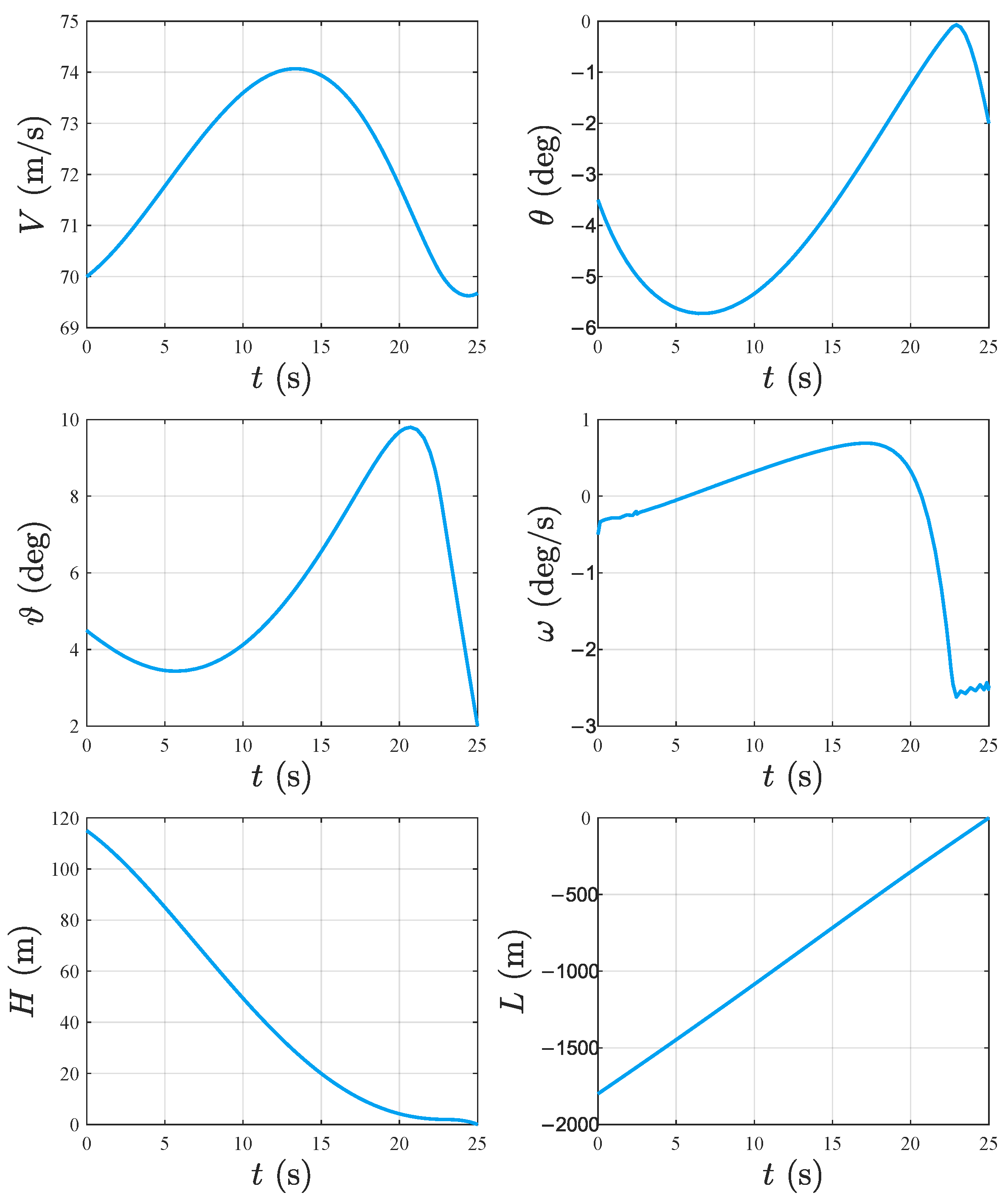
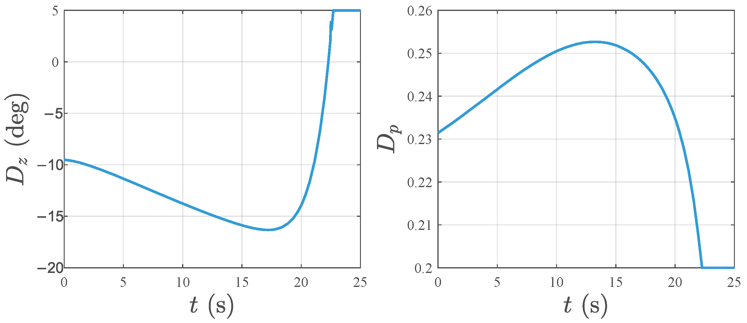
Range $L_0$	−1800 m	0 m

. The resulting nominal state and control trajectories, obtained using GPOPS-II, are shown in Figure 3 and Figure 4, respectively, with a total duration of 25 s. Relevant parameters for funnel computation are listed in

Table 3. Parameter settings for funnel computation.

Parameter	Value (Range)
Number of discretization points N	51
Closed-loop elevator deflection constraint, $D_z$	[$-20$, 10]°
Closed-loop throttle setting constraint, $D_p$	[0.1, 1]
Roll-back factor b	1.5
Convergence threshold for shape matrix $\epsilon$	0.02

.

The nominal state and control trajectories satisfy the initial and terminal constraints specified in Table 2. In particular, the altitude decreases to zero and the range approaches zero at the final time, while the terminal airspeed, flight-path angle, and pitch angle remain within their prescribed intervals. The state trajectories evolve continuously throughout the landing process, and the nominal elevator deflection and throttle setting remain within the control bounds imposed during trajectory planning. The relatively larger state and control variations near the terminal phase result from the simultaneous enforcement of the terminal position and attitude constraints.

The nominal state and control trajectories provide the reference centerline for all subsequent simulations. Specifically, they are used to construct the linear time-varying deviation model, compute the time-varying LQR gain, establish the closed-loop polynomial error dynamics, and define the nominal trajectory along which the five-dimensional and six-dimensional funnels are computed.

4.1. Effect of Polynomial-Model Accuracy on Go-Around Decisions

Conventional ACLS studies still commonly employ small-disturbance or locally linearized aircraft models, although nonlinear models have increasingly been adopted to better capture the nonlinear dynamics of carrier landing. In the present funnel computation, the first-order polynomial approximation is equivalent to such a local linearization, whereas the second-order approximation additionally retains the leading nonlinear terms. Therefore, this subsection investigates whether the accuracy of the linearized model is sufficient for constructing a reliable offline funnel decision boundary, or whether a second-order nonlinear approximation is necessary for the ACLS go-around decision problem considered in this study. To isolate the effect of polynomial-model accuracy from the effect of state dimensionality, both cases considered in this subsection use the same reduced five-dimensional formulation, in which the range state L is omitted. A first-order polynomial approximation and a second-order polynomial approximation are used to construct two five-dimensional funnels. The reliability of the resulting offline decision boundaries is then evaluated using trajectories propagated by the original closed-loop nonlinear system.

To provide a reduced benchmark consistent with conventional ACLS modeling practice, the five-state longitudinal formulation in [2] is adopted only for the comparative analysis in this subsection. The selected state variables are the scaled airspeed $v=V/V_0$, flight-path angle $\theta$, pitch angle $\vartheta$, pitch rate $\omega$, and scaled altitude $h=H/V_0$. The control inputs are the elevator deflection $D_z$ and throttle setting $D_p$. Here, $V_0$ denotes the initial airspeed of the nominal trajectory and is used as the scaling factor. The weighting matrices for the LQR controller are specified as

$${\mathit{Q}}_f=\mathit{Q}=\mathrm{diag}\left(\left[11111\right]\right),\mathit{R}=\mathrm{diag}\left(\left[11\right]\right).$$

The corresponding LQR controller is used to construct the closed-loop error dynamics. For the reduced five-dimensional formulation, the shape matrix of the terminal set is denoted by ${\mathit{E}}_5$ and specified as

$${\mathit{E}}_5=\mathrm{diag}\left(\left[{\displaystyle \frac{V_0^2}{4}}11{\displaystyle \frac{1}{4}}{V}_0^2\right]\right).$$

Accordingly, the terminal deviations relative to the nominal trajectory are required to remain within 2 m/s in airspeed, 1° in flight-path angle, 1° in pitch angle, 2°/s in pitch rate, and 1 m in altitude. These terminal bounds are selected as physically reasonable reference values to define the required landing precision for the numerical study. In practical applications, the terminal-set matrix can be adjusted according to the actual landing requirements, aircraft characteristics, and operational specifications.

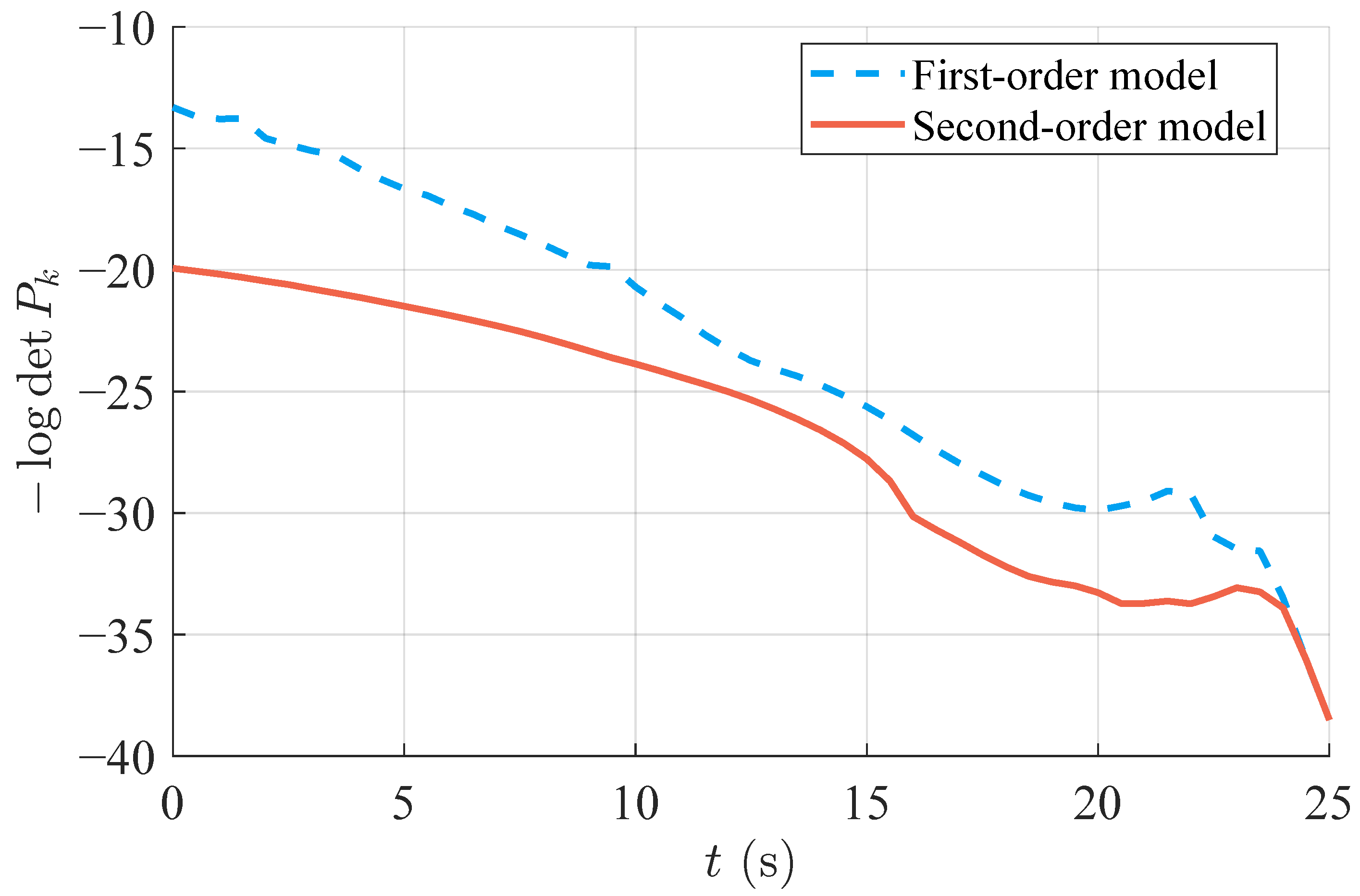
First-order and second-order polynomial approximations of the closed-loop error dynamics with respect to the state deviation are constructed using the same LQR controller. The time-varying sizes of the resulting five-dimensional funnels are shown in Figure 5. Since the volume of a funnel ellipsoid is proportional to ${\left(\det {\mathit{P}}_k\right)}^{-1/2}$, a larger value of $-log\det {\mathit{P}}_k$ represents a larger funnel at the corresponding time instant. Both funnels generally contract as the landing process approaches the prescribed terminal set. The funnel constructed using the first-order polynomial approximation is generally larger than that constructed using the second-order approximation. However, a larger funnel does not necessarily provide a more reliable decision boundary, because the neglected nonlinear terms may cause the first-order approximation to overestimate the safe region of the original closed-loop nonlinear system. 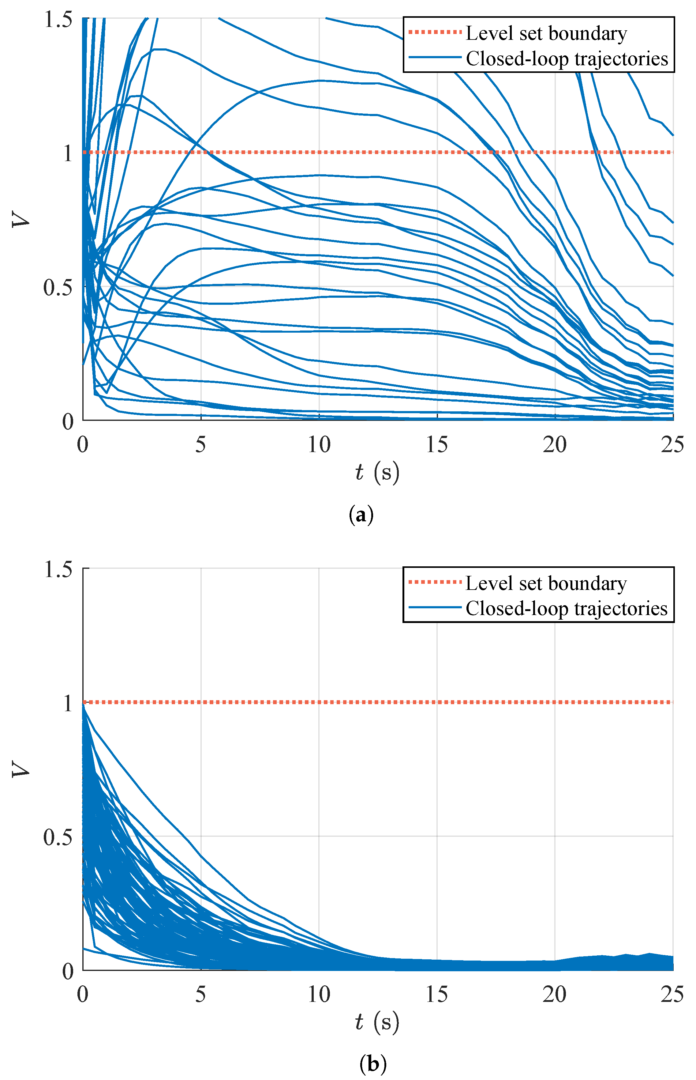This issue is further evaluated using the nonlinear closed-loop trajectories shown in Figure 6. At the entrance time $t_1=0$, 100 initial perturbation vectors are uniformly sampled within the five-dimensional funnel for each approximation case. Because these perturbation vectors lie in a five-dimensional state space, they are not directly displayed in Figure 5, which only presents the scalar quantity used to represent the funnel size. Starting from these initial states, the corresponding trajectories are propagated by numerically integrating the original closed-loop nonlinear system rather than using either polynomial approximation. Each blue curve in Figure 6 represents the level-set function history associated with one of the sampled initial perturbation vectors.

During each closed-loop simulation, the reduced five-dimensional version of the online go-around decision module operates at every sampling instant. Specifically, the module evaluates the current five-dimensional state deviation against the corresponding precomputed five-dimensional funnel and outputs either the continue-landing decision or the go-around decision according to the same membership rule as that in (35). Therefore, the level-set histories in Figure 6 directly evaluate whether the offline decision boundaries constructed from the two polynomial approximations remain valid when applied to the original closed-loop nonlinear system.

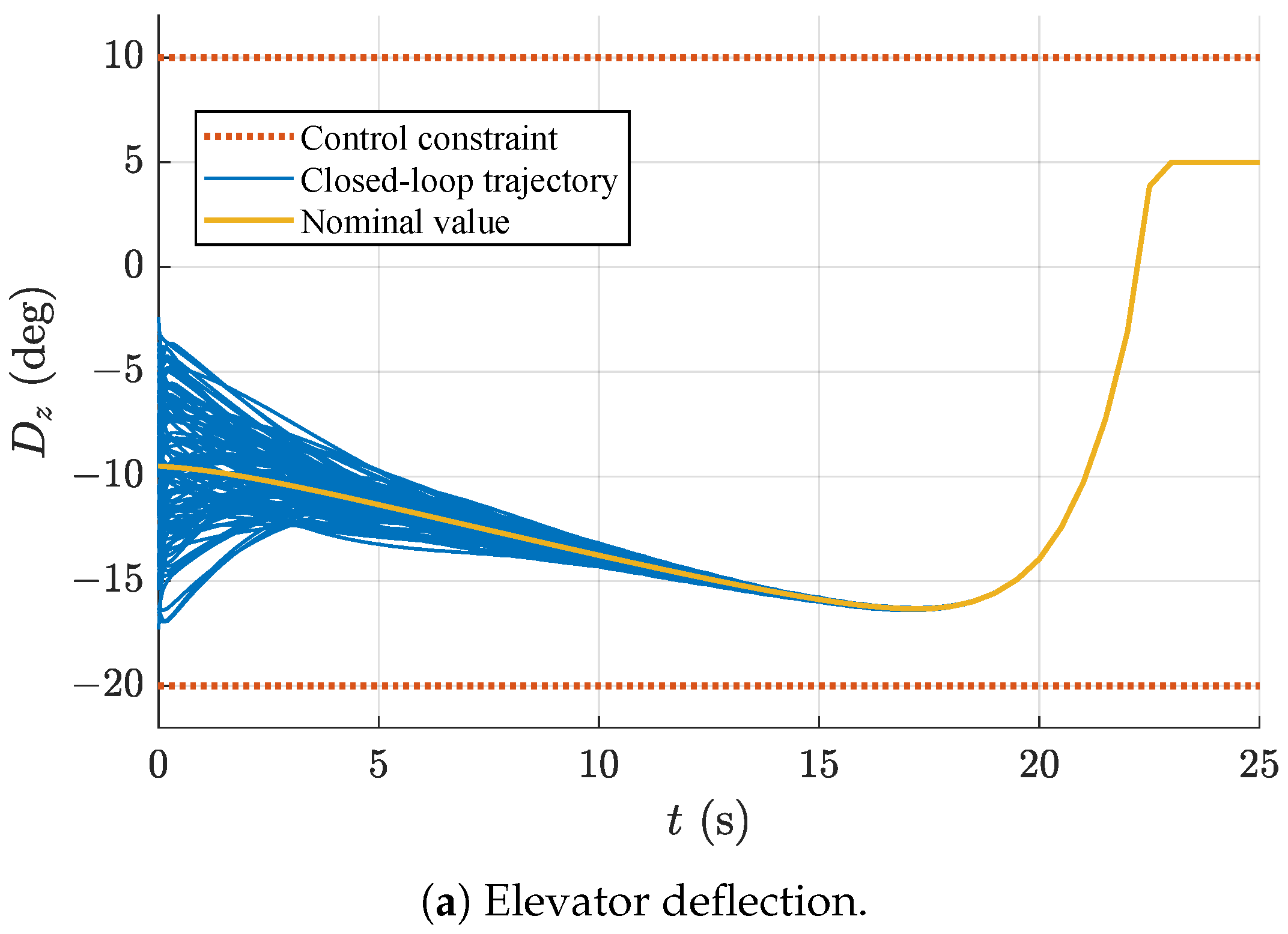
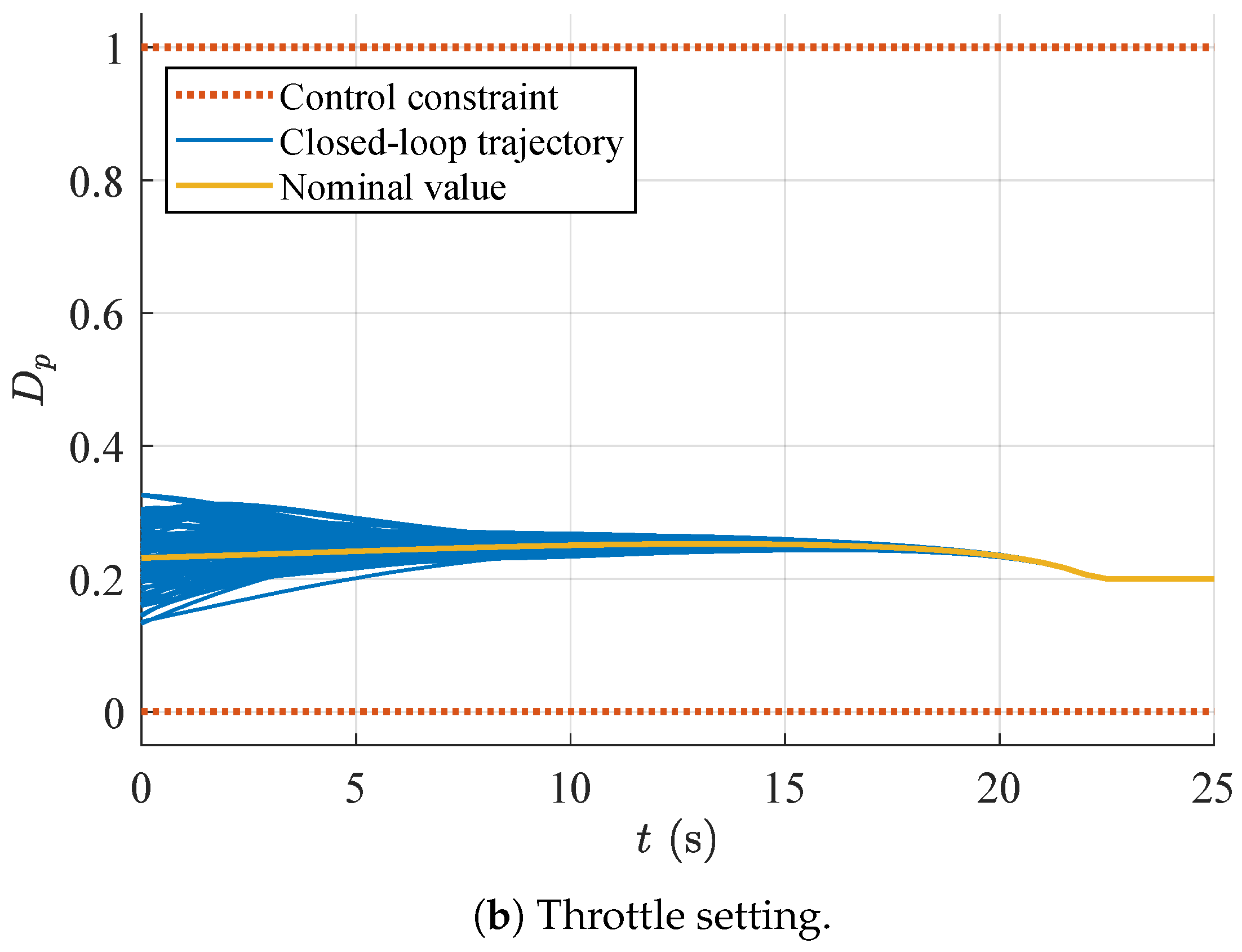
For the funnel constructed using the second-order closed-loop polynomial system, none of the level-set function values in Figure 6b exceed the funnel boundary $V_k=1$. Consequently, the online decision module continuously outputs the continue-landing decision throughout the simulation. All trajectories subsequently reach the prescribed five-dimensional terminal set at the final time, supporting the validity of these continue-landing decisions with respect to the reduced five-dimensional formulation. The corresponding elevator deflection and throttle setting are shown in Figure 7a and Figure 7b, respectively, and both remain within the saturation limits specified in Table 3.

For the funnel constructed using the first-order polynomial approximation, several trajectories of the original closed-loop nonlinear system in Figure 6a exceed the funnel boundary $V_k=1$. According to the go-around decision rule in (35), the online decision module outputs the go-around decision for each of these trajectories at the first sampling instant for which $V_k\left(\overline{\mathit{x}}\left(t_k\right)\right)>1$, because the guarantee that the trajectory will remain within the subsequent funnel and reach the prescribed terminal set is no longer available. Therefore, Figure 6a explicitly demonstrates the online transition from the continue-landing decision to the go-around decision. The trajectories are propagated beyond the triggering instant only to evaluate the discrepancy between the first-order closed-loop polynomial system and the original closed-loop nonlinear system. This continued propagation does not represent execution of the post-trigger go-around maneuver, which is outside the scope of this study. The first-order approximation produces a funnel that extends into regions farther from the nominal trajectory, where the nonlinear terms neglected by the approximation become significant. Consequently, the resulting funnel does not provide a reliable offline decision boundary for the original closed-loop nonlinear system.

Although the second-order polynomial model provides a reliable offline decision boundary with respect to the five modeled states, the reduced formulation does not evaluate the range state. Figure 8 and

Table 4. Terminal altitude and range dispersion statistics of the closed-loop trajectories (m).

Formulation	State	Mean	Max.	Standard Deviation
5D	Altitude H	0.213	0.582	0.154
5D	Range L	8.486	22.841	5.765
6D	Altitude H	0.069	0.207	0.052
6D	Range L	0.065	0.173	0.039

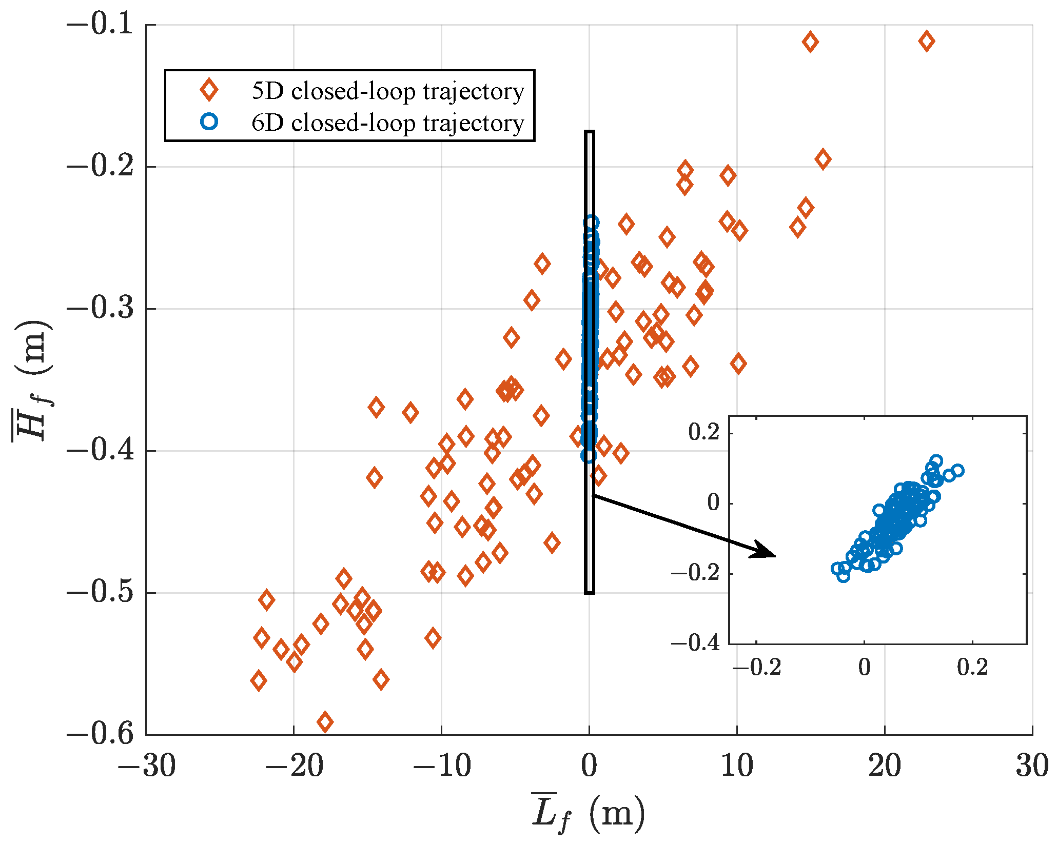
summarize the terminal altitude and range dispersions for the five-dimensional formulation considered in this subsection and the six-dimensional formulation introduced in Section 4.2. The present subsection focuses on the five-dimensional results. Although the terminal altitude remains within the corresponding terminal requirement, the terminal range exhibits large deviations, with some values exceeding 20 m. This occurs because the range state L is excluded from the five-dimensional formulation. Therefore, the continue-landing decisions based on the five-dimensional funnel are valid only with respect to the five modeled states and cannot guarantee satisfaction of the additional terminal range requirement considered in this study. This limitation motivates the incorporation of the range state and the construction of the six-dimensional funnel in the following subsection.

4.2. Effect of the Range State on Go-Around Decisions

The results in Section 4.1 show that a reliable five-dimensional decision boundary remains insufficient for evaluating the complete terminal set considered in this study because the range state is omitted. Therefore, this subsection incorporates the range state L into the state-feedback design, terminal set, and online membership test. The resulting six-dimensional funnel enables the online go-around decision module to evaluate the complete six-dimensional state deviation and determine whether the corresponding closed-loop trajectory is guaranteed to remain within the subsequent funnel and reach the prescribed terminal set, including the additional terminal range requirement considered in this study.

Consistent with the scaling adopted in Section 4.1, the range state is scaled as $l=L/V_0$. The six-dimensional state used for the funnel computation is therefore composed of the scaled airspeed $v=V/V_0$, flight-path angle $\theta$, pitch angle $\vartheta$, pitch rate $\omega$, scaled altitude $h=H/V_0$, and scaled range $l=L/V_0$. The weighting matrices for the LQR controller are specified as

$${\mathit{Q}}_f=\mathit{Q}=\mathrm{diag}\left(\left[111111\right]\right),\mathit{R}=\mathrm{diag}\left(\left[11\right]\right).$$

Based on the findings in Section 4.1, a second-order polynomial approximation of the resulting closed-loop error dynamics is constructed and used for the offline computation of the six-dimensional funnel. The shape matrix of the corresponding six-dimensional terminal set is specified as

$$\mathit{E}=\mathrm{diag}\left(\left[{\displaystyle \frac{V_0^2}{4}}11{\displaystyle \frac{1}{4}}{V}_0^2{\displaystyle \frac{V_0^2}{4}}\right]\right).$$

Accordingly, the terminal deviations relative to the nominal trajectory are required to remain within 2 m/s in airspeed, 1° in flight-path angle, 1° in pitch angle, 2°/s in pitch rate, 1 m in altitude, and 2 m in range.

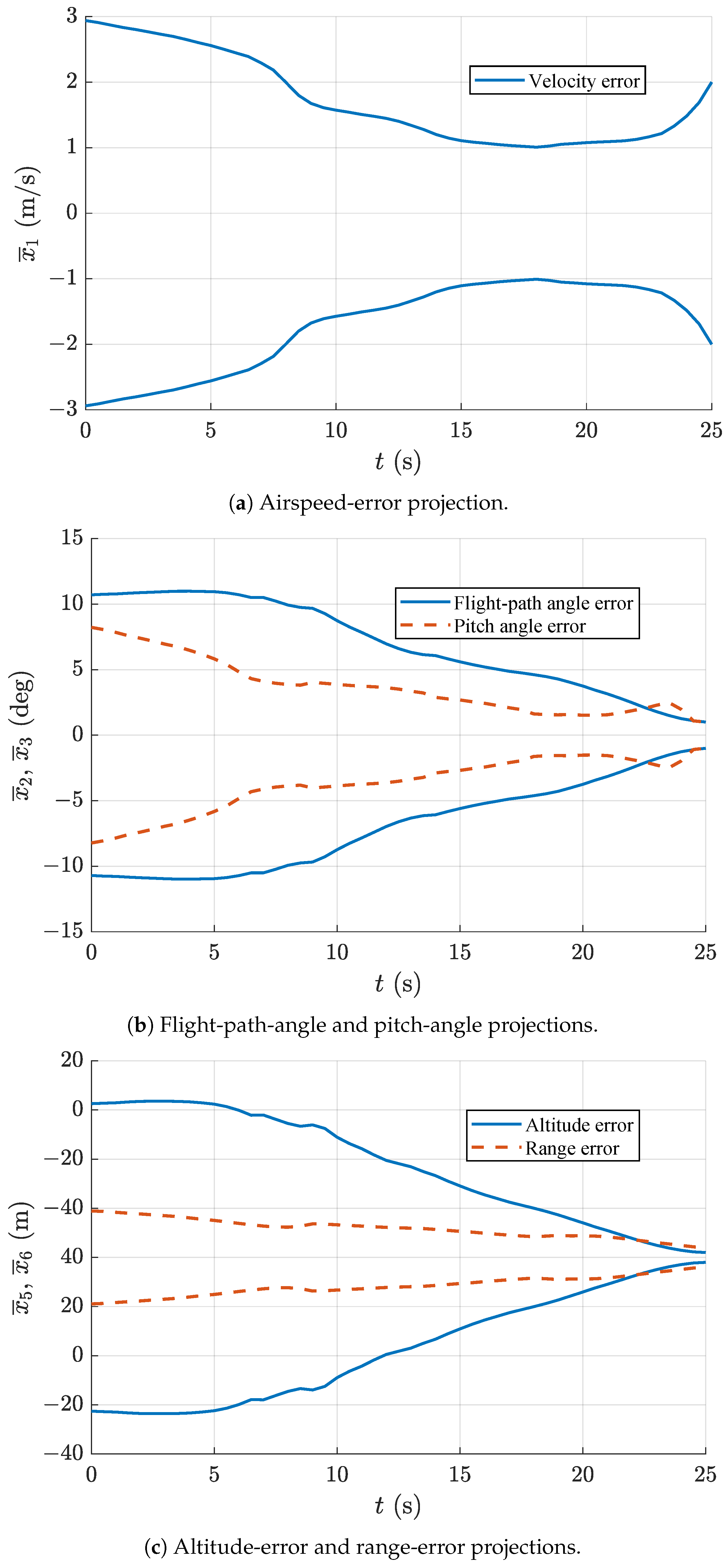
Figure 9 shows the one-dimensional projections of the resulting six-dimensional funnel onto selected state axes. The projections indicate that the offline-computed funnel entrance accommodates deviations of approximately 3 m/s in airspeed, 30 m in altitude, and 10 m in range along the corresponding coordinate directions. These values characterize the projections of the six-dimensional safe region and should not be interpreted as independent componentwise thresholds. As in Section 4.1, 100 initial perturbation vectors are uniformly sampled within the six-dimensional funnel at the entrance time $t_1=0$. Starting from these initial states, the corresponding trajectories are propagated using the original closed-loop nonlinear system. At every sampling instant, the online go-around decision module evaluates the complete six-dimensional state deviation according to (35).

Note 1. At a given time, a state component may lie within the corresponding one-dimensional funnel projection even though the complete six-dimensional state deviation lies outside the funnel. This is analogous to a point whose individual coordinates lie within the coordinate projections of a tilted ellipse, while the complete point still lies outside the ellipse. Therefore, the online go-around decision is made using the level-set function evaluated with the complete six-dimensional state deviation rather than any individual funnel projection.

Throughout the simulations, none of the sampled trajectories exceeds the six-dimensional funnel boundary. The online go-around decision module therefore continuously outputs the continue-landing decision. Figure 8 and Table 4 show that the trajectories subsequently satisfy both the terminal altitude and terminal range requirements. The statistics in Table 4 are used only to evaluate the terminal performance of the closed-loop trajectories and are not involved in the online go-around decision, which is made exclusively according to the six-dimensional funnel membership condition in (35). Moreover, all six terminal state deviations remain within the prescribed six-dimensional terminal set. These results support the validity of the continue-landing decisions under the considered conditions: the corresponding trajectories remain within the six-dimensional funnel and reach the prescribed terminal set, which encodes the required landing precision together with the additional terminal range requirement considered in this study.

For this five-dimensional versus six-dimensional comparison, the aircraft parameters, nominal trajectory, second-order polynomial approximation, actuator saturation constraints, terminal requirements for the five common states, and numerical settings are kept consistent. The formulation change is the incorporation of the range state and its corresponding terminal requirement into the state-feedback design, terminal set, and online membership test. Under this controlled comparison, incorporating the range state substantially reduces the terminal altitude and range dispersions. For altitude H, the mean, maximum, and standard deviation decrease from 0.213 m, 0.582 m, and 0.154 m to 0.069 m, 0.207 m, and 0.052 m, corresponding to reductions of approximately 68%, 64%, and 66%, respectively. For range L, the corresponding values decrease from 8.486 m, 22.841 m, and 5.765 m to 0.065 m, 0.173 m, and 0.039 m, representing reductions of approximately 99% in the mean, maximum, and standard deviation.

The five-dimensional benchmark adopted in Section 4.1 follows a conventional longitudinal tracking formulation centered on airspeed, flight-path and attitude variables, and altitude, in which range is not included as an independent feedback state. The present controlled comparison shows that, when terminal range accuracy is explicitly included in the landing requirements, incorporating the range state into the state-feedback design, terminal set, and online membership test can substantially improve terminal landing precision. Moreover, omission of the range state can result in a continue-landing decision even though the terminal range requirement is not satisfied. Consequently, the offline-computed six-dimensional funnel not only improves the terminal altitude and range performance under the considered simulation settings, but also enables the online go-around decision to account directly for the additional terminal range requirement.

4.3. Effect of Deck Motion on Go-Around Decisions

Based on the six-dimensional formulation established in Section 4.2, this subsection investigates the effect of deck motion on the offline-computed decision boundary and the corresponding online go-around decisions. Deck motion is treated as a representative carrier-specific bounded environmental disturbance within the prescribed bounded uncertainty framework established in Section 3.1.4 [34]. Its heave component directly changes the relative altitude between the aircraft and the carrier deck during the terminal landing phase. Therefore, deck motion is selected in this subsection to illustrate how a prescribed environmental disturbance affects the offline-computed six-dimensional funnel and the corresponding online go-around decisions. The prescribed heave component of deck motion is described as

$${\dot{h}}_{\mathrm{deck}}=1.219sin\left(0.6t+{\displaystyle \frac{\pi }{2}}\right)+{\displaystyle \frac{0.707\times 90}{57.3}}sin\left(0.6t\right).$$

From the perspective of the relative motion between the aircraft and the carrier deck, the heave component of deck motion is incorporated into the nonlinear longitudinal model. Accordingly, the altitude dynamics in (1) are modified as

$$\dot{H}=Vsin\theta -{\dot{h}}_{\mathrm{deck}}.$$

For the deck-motion case, the shape matrix of the six-dimensional terminal set is denoted by ${\mathit{E}}_{\mathrm{deck}}$ and specified as

$${\mathit{E}}_{\mathrm{deck}}=\mathrm{diag}\left(\left[{\displaystyle \frac{V_0^2}{4}}11{\displaystyle \frac{1}{4}}{\displaystyle \frac{V_0^2}{16}}{\displaystyle \frac{V_0^2}{4}}\right]\right).$$

Accordingly, the terminal deviations relative to the nominal trajectory are required to remain within 2 m/s in airspeed, 1° in flight-path angle, 1° in pitch angle, 2°/s in pitch rate, 4 m in altitude, and 2 m in range. The prescribed deck motion is incorporated during the interval from 22 to 25 s. Based on the modified nonlinear longitudinal dynamics, the corresponding closed-loop polynomial system is reconstructed and the six-dimensional funnel is recomputed offline. For the comparison in Figure 10, the funnels with and without deck motion are computed using the same terminal set ${\mathit{E}}_{\mathrm{deck}}$, LQR controller, actuator saturation constraints, polynomial approximation order, and numerical settings. Therefore, the presence of the prescribed deck motion is the only difference between the two cases.

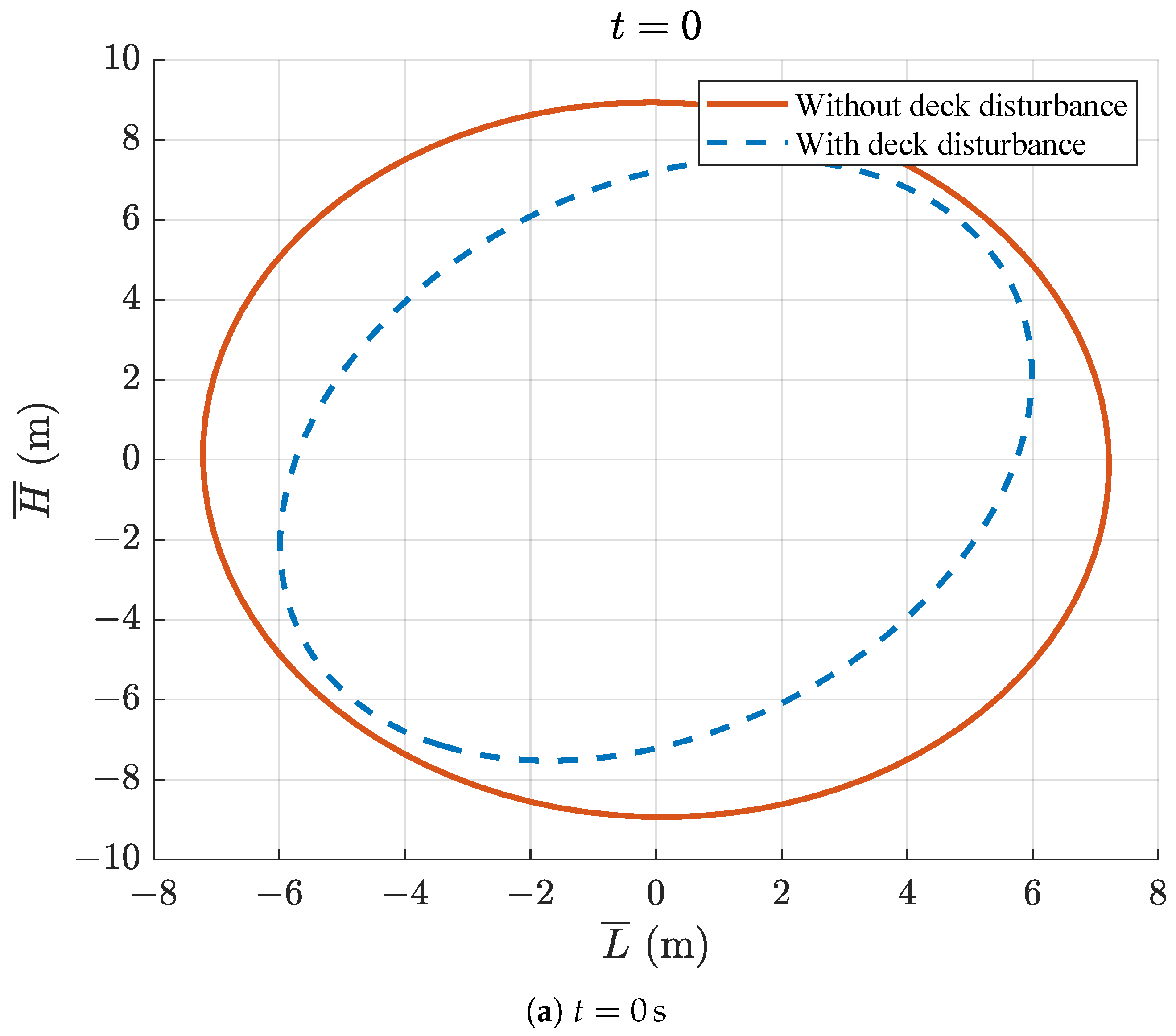
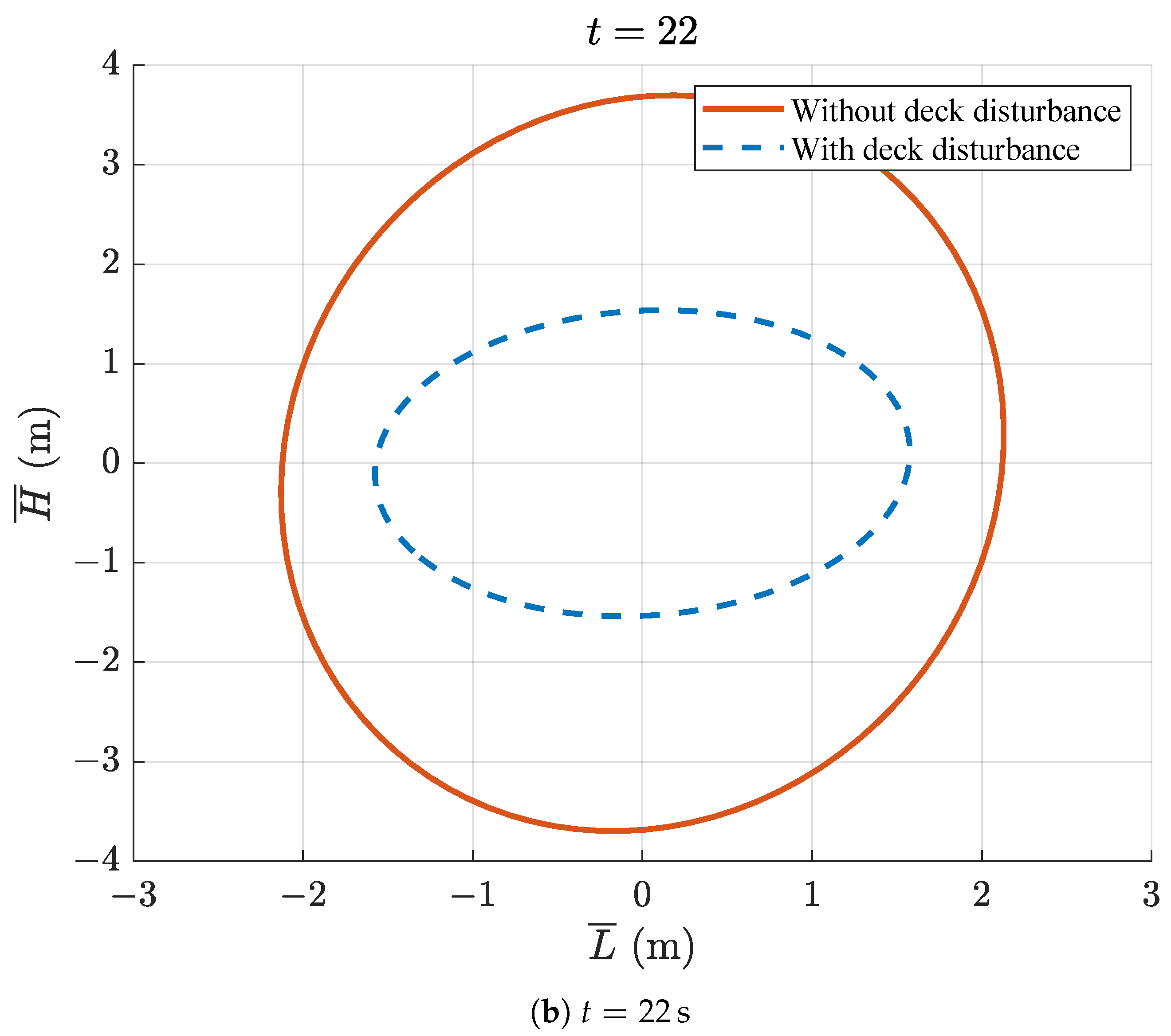
Figure 10 compares the altitude–range slices of the six-dimensional funnels computed with and without deck motion at $t=0$ s and $t=22$ s. These slices are used only to visualize the change in the offline-computed decision boundary. The actual continue-landing or go-around decision is still made by the online go-around decision module using the complete six-dimensional state deviation according to (35).

Note 2. Unlike the one-dimensional projections discussed in Section 4.2, the two-dimensional altitude–range slice in Figure 10 is obtained by setting the remaining four state deviations, namely the airspeed, flight-path-angle, pitch-angle, and pitch-rate deviations, to zero. Therefore, each point inside the slice, together with these four zero-valued state deviations, represents a complete six-dimensional state deviation inside the funnel. The slice is used only for visualization and does not replace the complete six-dimensional membership test performed by the online go-around decision module.

Figure 10 demonstrates how the proposed framework remains applicable after deck motion is incorporated into the nonlinear longitudinal model. The effect of deck motion is accounted for by recomputing the six-dimensional funnel offline, whereas the online go-around decision rule remains unchanged. As shown in Figure 10b, the six-dimensional funnel computed with deck motion is smaller at $t=22$ s than that computed without deck motion. Because the funnel is constructed backward from the terminal set, this reduction also propagates backward to the funnel entrance, as shown in Figure 10a. Therefore, the prescribed deck motion reduces the range of complete six-dimensional state deviations for which the continue-landing guarantee is available.

Under the considered deck-motion condition and the other conditions imposed during the offline computation, every complete six-dimensional state deviation inside the recomputed funnel is associated with a closed-loop trajectory that remains within the subsequent funnel, satisfies the actuator saturation constraints, and reaches the prescribed terminal set. These results demonstrate that the proposed method remains applicable under the prescribed deck-motion disturbance by updating the offline-computed decision boundary. Deck motion may change the online decision corresponding to a given complete six-dimensional state deviation because the precomputed funnel changes, but it does not change the go-around decision rule itself.

If the actual deck motion exceeds the prescribed bounds, the offline guarantee is no longer established. If the resulting complete six-dimensional state deviation leaves the recomputed funnel, the online go-around decision module detects the membership violation and outputs the go-around decision according to the same rule in (35).

4.4. Comparison with Altitude-Deviation-Based Go-Around Decisions

The six-dimensional funnel used in Figure 11 is the funnel recomputed offline under the prescribed deck-motion condition examined in Section 4.3. The comparison in this subsection is intended to isolate the effect of the go-around decision criterion rather than to reproduce a specific existing ACLS implementation. Accordingly, a representative altitude-deviation-based criterion, following the conventional decision principle summarized in [3], is implemented within the same aircraft model, nominal trajectory, feedback controller, and prescribed deck-motion condition as the proposed method, so that the two decision criteria are evaluated under identical conditions. The prescribed altitude-deviation band represents the continue-landing region admitted by this altitude-deviation-based benchmark, whereas the time-varying altitude–range slices of the recomputed six-dimensional funnel represent the corresponding continue-landing region provided by the proposed method when the remaining four state deviations are set to zero.

The relationship between the two decision regions can be interpreted in three cases. First, complete six-dimensional state deviations represented inside both regions lead both decision criteria to output the continue-landing decision. Second, the portions inside the recomputed funnel but outside the prescribed altitude-deviation band correspond to complete six-dimensional state deviations whose altitude components exceed the prescribed altitude-deviation threshold while the complete-state deviations remain inside the funnel. For these states, the altitude-deviation-based benchmark outputs the go-around decision, whereas the proposed online go-around decision module outputs the continue-landing decision because the corresponding closed-loop trajectories remain covered by the offline guarantee and reach the prescribed terminal set under the considered deck-motion condition. Therefore, the go-around decisions produced by the altitude-deviation-based benchmark in these portions are unnecessary under the considered conditions. Third, complete six-dimensional state deviations outside the recomputed funnel lie outside the safety-guaranteed continue-landing region, and the proposed online go-around decision module outputs the go-around decision because the continue-landing guarantee is no longer available.

It should also be emphasized that the altitude–range slices in Figure 11 are obtained by setting the other four state deviations to zero. Therefore, the fact that the prescribed altitude-deviation band lies within the displayed slices does not imply that every complete-state deviation satisfying the altitude threshold is safe for continued landing. When nonzero deviations in airspeed, flight-path angle, pitch angle, or pitch rate cause the complete six-dimensional state deviation to lie outside the funnel, the proposed module outputs the go-around decision even if the altitude deviation remains within the prescribed altitude-deviation band. Thus, compared with the altitude-deviation-based benchmark, the proposed rule can avoid unnecessary go-around decisions caused by reliance on a single-dimensional threshold while also identifying complete-state deviations for which the continue-landing guarantee is no longer available even when the altitude deviation remains within the prescribed threshold.

4.5. Effect of Required Landing Precision on Go-Around Decisions

This subsection investigates how the required landing precision affects the offline-computed six-dimensional decision boundary and the corresponding online go-around decisions. Three terminal sets are considered: the baseline terminal set defined by $\mathit{E}$, a stricter terminal set defined by $2\mathit{E}$, and a looser terminal set defined by $0.5\mathit{E}$. According to the terminal-set definition in (15), multiplying the terminal-set shape matrix by a positive scalar $\alpha$ scales each coordinate-axis radius of the terminal ellipsoid by $1/\sqrt{\alpha }$. For the baseline terminal set $\mathit{E}$ defined in Section 4.2, the corresponding coordinate-axis terminal deviation limits are 2 m/s in airspeed, 1° in flight-path angle, 1° in pitch angle, 2°/s in pitch rate, 1 m in altitude, and 2 m in range. Therefore, the stricter terminal set $2\mathit{E}$ reduces these limits to approximately 1.414 m/s, 0.707°, 0.707°, 1.414°/s, 0.707 m, and 1.414 m, respectively. Conversely, the looser terminal set $0.5\mathit{E}$ increases them to approximately 2.828 m/s, 1.414°, 1.414°, 2.828°/s, 1.414 m, and 2.828 m, respectively.

For each terminal set, the terminal funnel shape matrix is set to the corresponding terminal-set shape matrix, and the six-dimensional funnel is recomputed offline. The six-dimensional formulation, second-order closed-loop polynomial system, LQR controller, and actuator saturation constraints are kept unchanged from those used in Section 4.2. During online implementation, the online go-around decision module applies the same go-around decision rule in (35) to the corresponding precomputed funnel. Therefore, changing the required landing precision changes the offline-computed decision boundary but does not change the go-around decision rule itself.

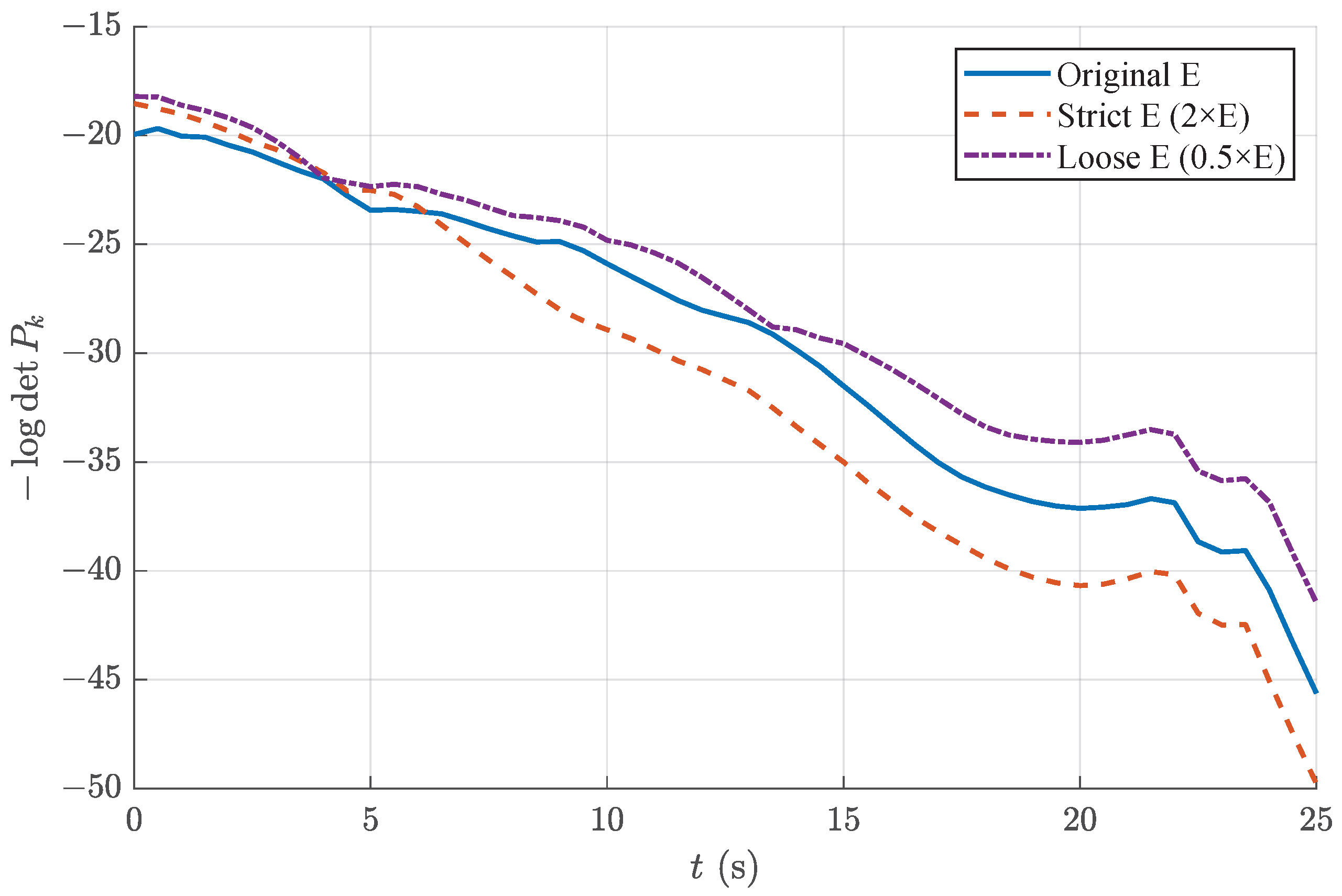
Figure 12 shows the time-varying sizes of the six-dimensional funnels corresponding to the three explicitly specified levels of required landing precision. Because the closed-loop dynamics, LQR controller, actuator saturation constraints, and prescribed uncertainty conditions are identical in the three cases, the differences among the curves are caused solely by the different terminal sets. The funnel computed for the looser terminal set $0.5\mathit{E}$, whose coordinate-axis terminal deviation limits are $\sqrt{2}$ times those of the baseline terminal set, has the largest size. In contrast, the funnel computed for the stricter terminal set $2\mathit{E}$, whose coordinate-axis terminal deviation limits are $1/\sqrt{2}$ times the baseline values, has the smallest size. The baseline funnel corresponding to $\mathit{E}$ lies between these two curves. The differences among the three funnels are relatively small during the initial interval of approximately 0–5 s, suggesting that the actuator saturation constraints on the elevator deflection and throttle setting have a stronger influence on the funnel size during this stage. After approximately 5 s, the effect of the selected terminal set becomes increasingly significant, and the ordering among the three curves becomes more pronounced. Thus, Figure 12 directly demonstrates that stricter required landing precision produces a smaller six-dimensional safe region, whereas looser required landing precision produces a larger one.

Under the conditions considered in the offline computation, the six-dimensional funnel contains the complete six-dimensional state deviations whose corresponding closed-loop trajectories remain within the subsequent funnel, satisfy the actuator saturation constraints, and reach the selected terminal set. Consequently, imposing stricter required landing precision reduces the size of the safe region for which the continue-landing guarantee is available, whereas imposing looser required landing precision enlarges this region.

At each sampling instant, the online go-around decision module evaluates the complete six-dimensional state deviation using the funnel computed for the selected terminal set. A given complete six-dimensional state deviation may lie inside the funnel computed for the looser terminal set $0.5\mathit{E}$ but outside the funnel computed for the stricter terminal set $2\mathit{E}$. In the former case, the online go-around decision module outputs the continue-landing decision because the corresponding closed-loop trajectory remains covered by the guarantee for reaching the looser terminal set. In the latter case, the guarantee for reaching the stricter terminal set is no longer available, and the online go-around decision module outputs the go-around decision. Thus, the same complete six-dimensional state deviation may produce different online decisions under different levels of required landing precision, even though the online go-around decision rule remains unchanged.

These results demonstrate that the proposed funnel-based method explicitly captures the trade-off between the required landing precision and the safe region size of the control system. A looser terminal set produces a larger six-dimensional funnel and allows the continue-landing guarantee to remain available for a wider range of complete six-dimensional state deviations. In contrast, a stricter terminal set produces a smaller six-dimensional funnel and reduces the range of complete six-dimensional state deviations for which the continue-landing guarantee is available. Therefore, the proposed method not only provides a quantitative tool for assessing the safe region size of the control system under a given required landing precision, but also provides the corresponding offline decision boundary required for implementing the go-around decision rule online.

5. Conclusions

This paper proposes a safety-guaranteed go-around decision framework for ACLSs based on an offline-computed six-dimensional funnel along the nominal landing trajectory. The results provide several findings regarding how the go-around decision can be formulated using the complete-state safe region and how the corresponding decision boundary is affected by the modeled dynamics, operating conditions, and landing requirements. The main conclusions are as follows:

(1)

The results show that the go-around decision can be formulated as a complete-state membership problem in a time-varying safe region rather than as a comparison between a single altitude deviation and a prescribed threshold. The offline-computed six-dimensional funnel incorporates the closed-loop dynamics, actuator saturation constraints, terminal landing requirements, and prescribed bounded uncertainties into the decision boundary. During online implementation, only the complete six-dimensional state deviation and the corresponding quadratic level-set function need to be evaluated. This provides a practical means of introducing a complete-state go-around decision criterion into an existing ACLS without requiring online SOS optimization or funnel recomputation.

(2)

The controlled comparison between the five-dimensional and six-dimensional formulations shows that explicitly incorporating the range state can substantially improve terminal landing precision. In the proposed six-dimensional formulation, the range state and its corresponding terminal requirement are incorporated into the state-feedback design, terminal set, and online membership test. Under the considered simulation settings, the mean, maximum, and standard deviation of the terminal altitude deviations are reduced by approximately 68%, 64%, and 66%, respectively, while the corresponding terminal range-deviation statistics are reduced by approximately 99%. These results demonstrate the benefit of explicitly including the range state when terminal range accuracy is incorporated into the complete-state go-around decision formulation.

(3)

The results further show that the go-around decision boundary is not a fixed geometric threshold but depends on the fidelity of the closed-loop model, the prescribed disturbance condition, and the required landing precision. The first-order approximation can overestimate the valid continue-landing region of the original closed-loop nonlinear system, whereas the second-order approximation provides a more reliable boundary under the considered conditions. Deck motion reduces the available continue-landing region and can be incorporated by recomputing the funnel offline, while stricter terminal requirements also reduce the funnel size. Compared with the representative altitude-deviation-based criterion considered in this study, the complete-state funnel provides additional decision information: it can avoid unnecessary go-around decisions when the altitude deviation exceeds the prescribed threshold while the complete state remains inside the funnel, and it can also identify complete-state deviations for which the continue-landing guarantee is no longer available even when the altitude deviation remains within the prescribed threshold.

These findings should be interpreted within the scope of the formulated guarantee. The safety guarantee is established for the adopted closed-loop longitudinal dynamics, actuator saturation constraints, terminal landing requirements, and prescribed bounded uncertainty set. The present numerical study uses deck motion as a representative carrier-specific environmental disturbance, whereas other bounded environmental effects, such as atmospheric disturbances, can be incorporated through the same prescribed bounded uncertainty formulation when their corresponding models and admissible bounds are specified. The reliability of the offline-computed decision boundary also depends on the accuracy of the polynomial approximation, which is why the first- and second-order approximations are explicitly evaluated against the original closed-loop nonlinear system. If the actual uncertainty exceeds the prescribed bounds, the guarantee is no longer established. Therefore, the proposed framework provides an explicit complete-state continue-landing region under specified modeling and operating conditions rather than an unconditional safety guarantee beyond these conditions. Joint optimization of the feedback controller and the funnel can further enlarge the safe region of the closed-loop system and remains a direction for subsequent development.