Preview-Aware LSTM-Assisted Predictive Control for Turboshaft Engines Under Tiltrotor Conversion-Flight Power Demand

Abstract

Conversion flight turns the aerodynamic versatility of a tiltrotor into a demanding propulsion-control problem. As the nacelles rotate and vertical load transfers from the proprotors to the wing, the two turboshaft engines must follow a rapidly changing shaft-power demand while respecting fuel command magnitude and rate limits, compressor-pressure limits and turbine temperature limits. A control-oriented conversion model is coupled to a component-level turboshaft engine through a long short-term memory (LSTM) dynamic surrogate embedded in a constrained receding-horizon controller. The aircraft model resolves wing force balance, blade-element/momentum rotor loads, forward acceleration, nacelle actuation and accessory power. The LSTM predicts six engine outputs from flight conditions, fuel command and previous-step spool speeds. Training and evaluation use 537 converged component model cases divided by complete simulation cases into 375 training, 80 validation and 82 held-out test cases. Against parameter-matched multilayer perceptron, temporal convolutional network and gated recurrent unit baselines, the LSTM gives the lowest power root-mean-square error (20.15 kW before online output correction). Its corrected 20–320-step forecasts outperform a linear autoregressive model and zero-order hold prediction, although the linear model remains slightly better at one step. In direct component-level closed-loop simulation, LSTM engine-surrogate nonlinear model predictive control (NMPC) reduces power RMSE from 29.80 to 16.23 kW relative to linear MPC and from 34.94 to 16.23 kW relative to PI control while reducing cumulative fuel command variation by 46.5% relative to linear MPC. Turbine temperature and compressor-pressure margins remain 119.0 K and 85.4 kPa, respectively. Mean optimization time is 29.6 ms for a 1.92 s update interval. The resulting framework connects conversion flight aerodynamic loading, multi-step engine prediction and constrained power control in a reproducible numerical validation chain.

1. Introduction

Tiltrotor aircraft combine vertical take-off and landing with wing-borne cruise by rotating proprotors between helicopter and airplane orientations. The XV-15 programme showed that this configuration can bridge the speed and range gap between conventional helicopters and fixed-wing aircraft [1]. The benefit is obtained through a conversion maneuver in which rotor thrust, wing lift, fuselage attitude and nacelle angle are continuously redistributed. A longitudinal tiltrotor model consequently has at least three dynamically distinct regions rather than two disconnected endpoints [2]. Rotor-wing and rotor-empennage interactions can also move conversion-corridor boundaries and alter trim power, particularly at low speeds where rotor download remains important [3].

Conversion is demanding for propulsion because the engine does not see nacelle angle alone. Forward acceleration increases the propulsive work rate, wing loading evolves with dynamic pressure, blade sections experience changing axial and in-plane velocity components, and nacelle actuation adds a smaller but finite mechanical load. Control-oriented tiltrotor studies have represented these effects using nonlinear rigid-body models and tilt angle-scheduled dynamics [4]. Trajectory optimization has further shown that required power, conversion time, control rate and corridor constraints must be considered together when choosing a nacelle schedule [5]. High-fidelity computations confirm that tilting rate and horizontal acceleration alter rotor-wing unsteadiness and may cause a nominal conversion trajectory to exceed the available-power boundary [6]. These findings imply that a credible engine-control experiment requires a power demand model that responds to blades, wing and flight kinematics, not a scalar nacelle angle correlation.

Blade-element/momentum theory (BEMT) offers an intermediate level of fidelity for that purpose. It resolves local blade velocity, angle of attack, sectional lift and drag and integrates their thrust and torque contributions while retaining a computational cost compatible with repeated control studies. A robust BEMT formulation has been shown to avoid singularities over mixed axial and in-plane inflow conditions and to support numerical rotor design [7]. BEMT does not reproduce every unsteady wake or compressibility effect, yet it creates a traceable link from blade geometry to shaft power and exposes the variables that a nacelle-only correlation suppresses.

The propulsion-control literature provides a second line of evidence. An integrated tiltrotor/turboshaft model with radial-basis-function feedforward control demonstrated that aircraft-induced load information can improve power turbine speed regulation, including hardware-in-the-loop tests [8]. Integrated helicopter/turboshaft studies have likewise used required-versus-delivered torque to coordinate rotor and engine dynamics [9]. More recently, an onboard composite helicopter/turboshaft system combined a neural inverse model with online optimization of rotor speed to reduce mission fuel consumption [10]. These studies establish the value of airframe-propulsion information exchange, but they do not directly answer how a recurrent multi-output engine-surrogate affects constrained power tracking during a continuous tiltrotor conversion.

Accurate control-oriented engine models remain a key challenge. A review by Wei and Zhang at Beihang University and Jafari and Nikolaidis at Cranfield University showed that onboard gas turbine models must balance transient fidelity, computational burden, lifecycle adaptation and runtime assurance [11]. Xu and co-workers at Xi’an Jiaotong University combined a physics-based model with self-tuning input-output models to reduce engine model mismatch using simulated-flight and ground-test data [12]. Paniccia and co-workers recently trained a supervised turboshaft dynamic model using real-flight records [13]. These studies motivate data-efficient onboard prediction while also showing that component-level simulation supports algorithm development but cannot replace independent rig or flight data calibration.

Model predictive control (MPC) is attractive because it converts a dynamic prediction into an explicit finite-horizon trade-off between tracking, control movement and constraints. The classical survey by Garcia et al. established the receding-horizon structure [14]. Mayne et al. formalized the stability and optimality questions that arise in constrained MPC [15]. Qin and Badgwell documented how prediction horizons, move suppression and model mismatch determine industrial implementations [16]. For aircraft engines, semi-alternative optimization has reduced the online burden of nonlinear MPC while retaining constraint handling [17], and subspace-updated prediction has enabled direct-performance adaptive control over changing operating points [18]. Turboshaft NMPC has also been applied to double-engine torque matching, where simultaneous speed and thermal constraints must be respected [19].

The prediction model inside MPC is therefore not a cosmetic choice. Jung et al. showed how LSTM networks can serve as dynamic MPC models, including mismatch correction, derivative evaluation and real-time implementation issues [20]. The original LSTM introduced gated memory to preserve information over long sequences [21], and the forget gate improved continual prediction [22]. Comparative analysis across LSTM variants has shown that performance depends on gate structure and task rather than on a universal architectural advantage [23]. Gated recurrence is especially relevant to gas turbines because spool inertia, thermal storage and actuator history make equal instantaneous inputs compatible with different future outputs. It also addresses the long-gradient difficulty that limits ordinary recurrent networks [24]. Interpretability is nevertheless important in a safety-relevant surrogate, motivating SHAP feature importance analysis based on the unified additive-explanation framework [25].

Alternative nonlinear controllers remain valuable benchmarks. Incremental nonlinear dynamic inversion has been developed for rapid turboshaft regulation [26], while integrated helicopter/turboshaft state-feedback control provides another route to coordinated engine-rotor dynamics [27]. Neural surrogates have also been used to accelerate aero-engine thrust estimation and control evaluation [28]. The scientific contribution is an integrated chain rather than a claim that MPC or LSTM is itself new: a blade-resolved conversion demand model is coupled to a multi-output LSTM engine-surrogate inside constrained NMPC, and the complete architecture is evaluated directly against a nonlinear component-level engine. The experiments ask whether LSTM is justified against GRU, temporal-convolution and multilayer-perceptron baselines; whether its multi-step errors remain controlled under input perturbations and rare events; whether conversion flight demand remains inside the learned engine domain; and whether improved engine prediction produces a measurable closed-loop benefit without relaxing engine or actuator constraints.

2. Integrated Engine-Surrogate Predictive Control Framework

2.1. Separation of Aircraft Demand and Engine Prediction

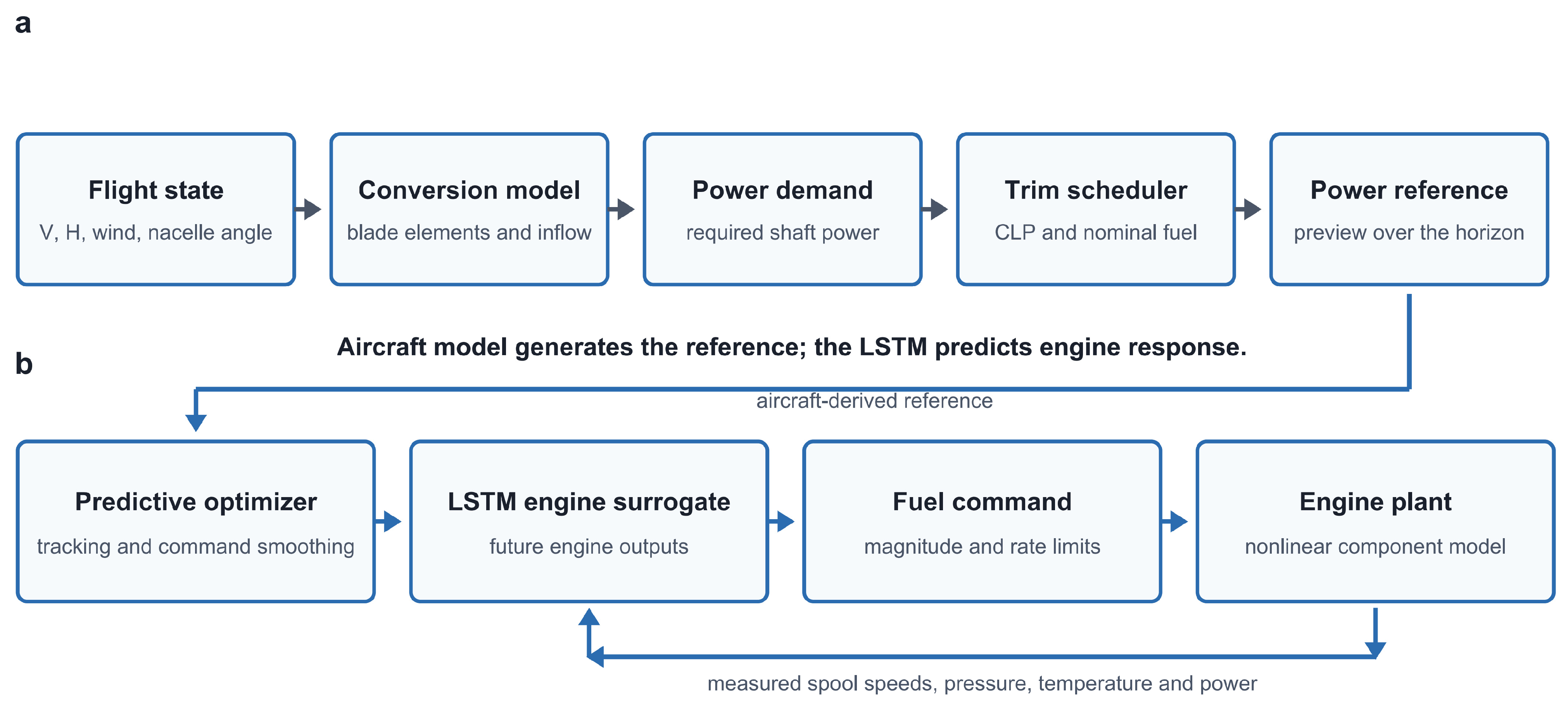
Figure 1 separates the conversion flight demand calculation from engine dynamic prediction. The aircraft demand module transforms speed, altitude, wind, sideslip and nacelle motion into per-engine required shaft power over the prediction horizon. The LSTM engine-surrogate maps operating condition, fuel command and previous-step power turbine and gas-generator speeds to future engine outputs. A supervisory trim scheduler maps required power to a feasible collective pitch lever (CLP) angle and nominal fuel command using converged steady component model nodes. PI control, linear MPC and LSTM engine-surrogate NMPC receive the same power reference, trim schedule and constraints; they differ in feedback structure and in the prediction model used by the optimizer.

The component-level turboshaft engine remains the controlled plant in every closed-loop comparison. It contains nonlinear compressor, combustor, gas-generator turbine, power turbine, shaft and gas path relationships. The controller receives corrected power turbine speed, corrected gas-generator speed, compressor-discharge total pressure, turbine temperature and shaft power through a one-sample measurement delay. Fuel is the manipulated variable. This direct plant-in-the-loop configuration is materially different from comparing controllers on a linear state-space plant.

2.2. Component-Level Data and LSTM Engine-Surrogate

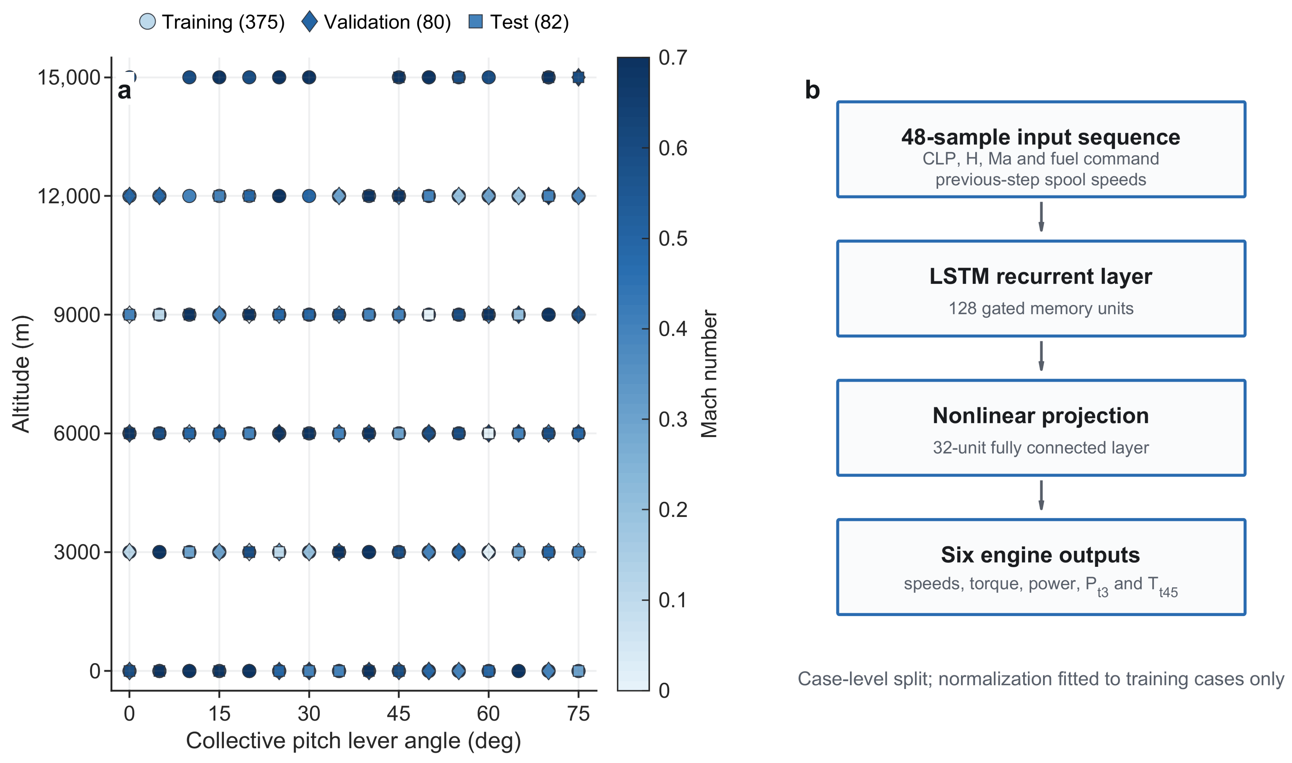
Engine simulations were generated on a three-factor full-combination numerical operating condition grid with CLP from 0 to 75 deg in 5 deg increments, altitude from 0 to 15,000 m in 3000 m increments, and Mach number from 0 to 0.7 in 0.1 increments. The grid contains 768 combinations. Component matching converged for 537 cases; failed points were retained in the numerical design record but excluded from learning because they do not define valid engine trajectories. Each converged case contains a fuel excitation and 3967 samples. Complete cases, rather than individual time samples, were assigned to training, validation and testing, preventing neighbouring samples from the same transient from leaking across subsets.

The input and output vectors are

$${{\mathbf{z}}_k}^T=\left[CL{P}_k,H_k,M{a}_k,W_{f,k},n_{pcr,k-1},n_{gcr,k-1}\right]$$

(1)

$${{\mathbf{y}}_k}^T=\left[n_{pcr,k},n_{gcr,k},M_{kp,k},P_k,P_{t3,k},T_{t45,k}\right]$$

(2)

where CLP is the engine collective pitch lever command, H is altitude, Ma is Mach number, Wf is the fuel command, n_pcr and n_gcr are corrected power turbine and gas-generator speeds, M_kp is output torque, P is shaft power, P_t3 is compressor-discharge total pressure and T_t45 is turbine temperature. The input sequence contains 48 consecutive sampling instants, corresponding to 1.152 s at the 0.024 s engine sampling interval. The network contains one 128-unit LSTM layer, a 32-unit dense layer, a hyperbolic-tangent projection and a six-unit regression output. The final network uses random seed 20260828, Adam optimization, a mini-batch size of 12, an initial learning rate of 8 × 10⁻⁴ halved every 10 epochs, a unit gradient threshold, validation every 20 iterations and validation patience of eight checks for at most 30 epochs. Input and output normalization are fitted on the training cases only. Network size and training parameters were selected from prespecified candidate configurations according to validation-set error. The resulting network and controller settings are summarized in

Table 1. Reproducibility parameters for engine learning and predictive control.

Item	Value	Comment
Engine sample interval	0.024 s	Component model and LSTM
LSTM input window	48 samples (1.152 s)	Six channels
LSTM architecture	128 LSTM; 32 dense; tanh; 6 outputs	20,454 parameters in matched model
Final LSTM training	Adam; 30 epochs; batch 12; lr 8 × 10−4	lr × 0.5 every 10 epochs; gradient limit 1
Validation/seed	frequency 20; patience 8; seed 20260828	Best validation-loss network
Data split	375/80/82 cases	Training/validation/held-out test
Controller update	1.92 s	80 plant samples
Prediction horizon	320 samples (7.68 s)	Four prediction blocks
Control horizon	2 block moves	Warm-started QP
LSTM NMPC weights	QP = 1; Rdelta = 6; Ru = 0.04	Power/increment/trim-level
Linear MPC weights	QP = 1; Rdelta = 12; Ru = 0.08	Same reference and constraints
Fuel command constraints	343–393; |rate| ≤ 2 unit s−1	Command magnitude/rate
Output constraints	Tt45 ≤ 1120 K; Pt3 ≤ 1320 kPa	Temperature/pressure

.

The LSTM gates and state update are written as follows, with sigma denoting the logistic function, the Hadamard product denoted by the circle-dot operator, W and U denoting input and recurrent weights, and b denoting biases.

$$i_k=\sigma \left(W_i{z}_k+U_i{h}_{k-1}+b_i\right)$$

(3a)

$$f_k=\sigma \left(W_f{z}_k+U_f{h}_{k-1}+b_f\right)$$

(3b)

$$o_k=\sigma \left(W_o{z}_k+U_o{h}_{k-1}+b_o\right)$$

(3c)

$$g_k=\mathit{tanh}\left(W_g{z}_k+U_g{h}_{k-1}+b_g\right)$$

(3d)

$$c_k=f_k\odot c_{k-1}+i_k\odot g_k,h_k=o_k\odot \mathit{tanh}\left(c_k\right)$$

(4)

2.3. Constrained Predictive Control

At each controller update, the measured output is appended to the LSTM history. A two-pass fixed-point rollout feeds predicted spool speeds into the previous-step speed inputs at subsequent prediction instants. The current one-step model mismatch is then held as an additive output correction over the horizon, a standard offset-compensation mechanism that prevents a small local bias from accumulating. The aircraft model independently supplies the required power sequence.

The additive output correction used during the multi-step rollout is

$${{\mathbf{y}}_{k+i}}^{corr}={{\mathbf{y}}_{k+i}}^{LSTM}+\left({\mathbf{y}}_k-{{\mathbf{y}}_k}^{LSTM}\right)$$

(5)

The finite-horizon objective penalizes required power tracking, fuel command increments and departure from the scheduled trim fuel:

$$\begin{array}{c}J={\displaystyle {{\displaystyle \sum }}_{i=1}^{N_p}}{Q}_P{\left|\right|P_{k+i}-P_{ref,k+i}\left|\right|}^2\\ +{\displaystyle {{\displaystyle \sum }}_{i=0}^{N_c-1}}{R}_{\Delta }{\left|\right|\Delta W_{f,k+i}\left|\right|}^2\\ +{\displaystyle {{\displaystyle \sum }}_{i=0}^{N_c-1}}{R_u\left|\right|W_{f,k+i}-W_{f,trim,k+i}\left|\right|}^2\end{array}$$

(6)

The input and engine output constraints are

$$\begin{array}{c}{W}_{f,min}\le W_{f,k+i}\le W_{f,max},\left|\Delta W_{f,k+i}\right|\le \Delta W_{f,max}\\ T_{t45,k+i}\le T_{t45,max},P_{t3,k+i}\le P_{t3,max}\end{array}$$

(7)

The plant sampling interval is 0.024 s. The controller is updated every 1.92 s, and the prediction horizon contains 320 plant samples or 7.68 s. Four 1.92 s prediction blocks are used; two block moves are optimized. For the selected LSTM engine-surrogate NMPC, QP = 1, Rdelta = 6 and Ru = 0.04. The linear MPC comparison uses QP = 1, Rdelta = 12 and Ru = 0.08. Finite-difference perturbations of the recurrent rollout construct local power, temperature and pressure sensitivities; the resulting quadratic programme is solved with warm starting. This sequential local approximation motivates the term LSTM engine-surrogate NMPC rather than a claim of globally solved nonlinear optimization.

The numerical fuel command is constrained to 343–393 command units and its rate to 2 command units per second. Because the component model does not provide an actuator-calibrated conversion from this command to physical mass flow, the rate limit is a simulation constraint rather than a certified fuel-control-unit limit. Tt45 and Pt3 are constrained to 1120 K and 1320 kPa, respectively. Identical limits are imposed on all predictive controller comparisons.

The existence of a finite-horizon minimizer follows at each feasible update because the fuel command and fuel increment constraints define a closed and bounded feasible set, while the LSTM maps, local prediction functions and quadratic cost are continuous. The Weierstrass theorem therefore ensures that a minimum exists whenever the feasible set is non-empty. This argument does not prove recursive feasibility, asymptotic closed-loop stability or global optimality; no terminal invariant set or Lyapunov terminal penalty is imposed.

3. Tiltrotor Conversion Flight Power-Demand Model

3.1. Conversion Profile and Wing-Rotor Force Coordination

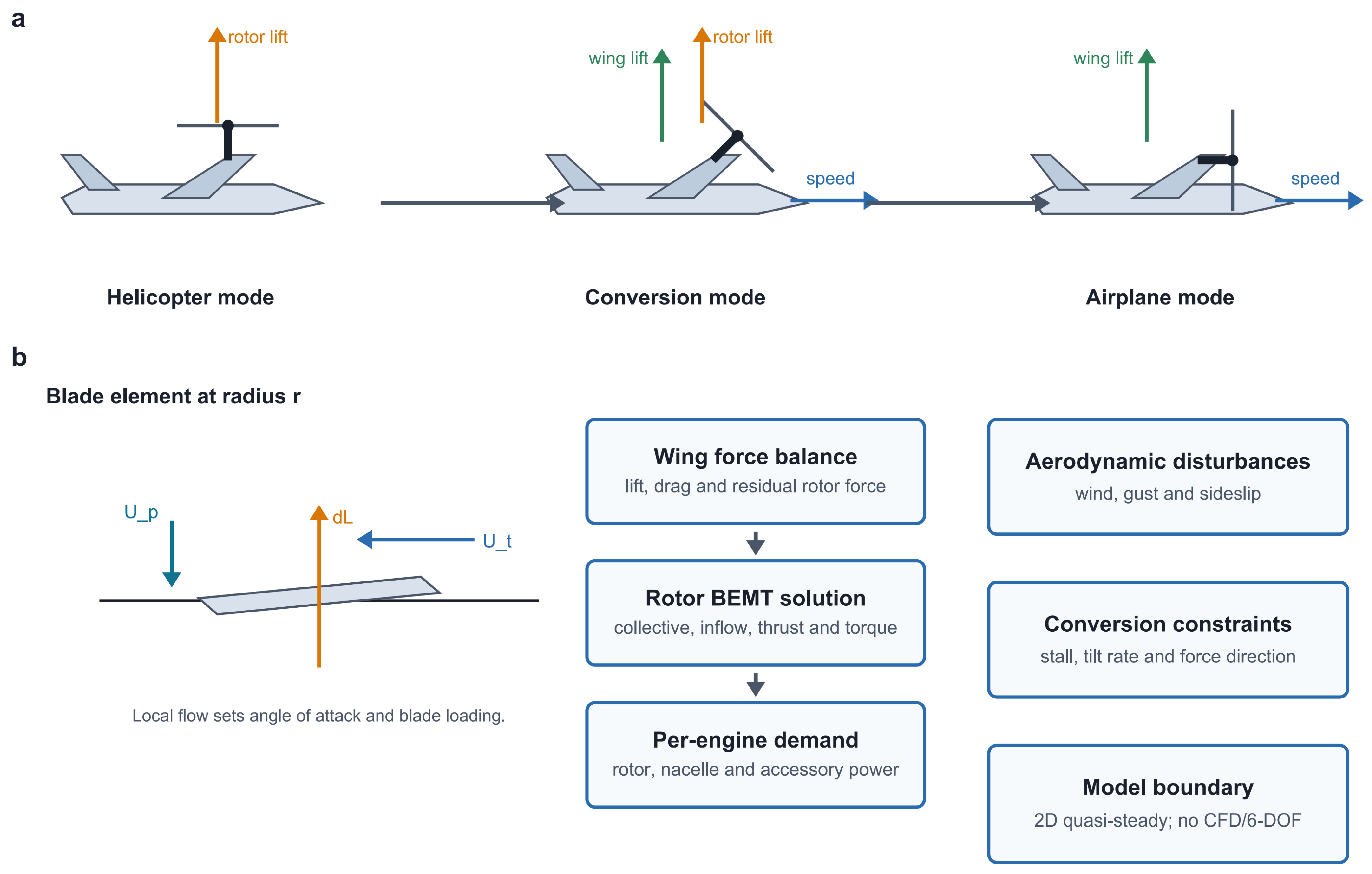
The conversion model is deliberately longitudinal but no longer relies on a prescribed rotor/wing lift-share correlation. Ground speed rises smoothly from 6 to 80 m s⁻¹, while the commanded nacelle angle changes from 90 deg to 0 deg. A fifth-order smooth-step schedule avoids discontinuities in acceleration and commanded tilt rate. The baseline case is level at sea level; additional cases impose plus or minus 10 m s⁻¹ longitudinal wind, 10 m s⁻¹ crosswind, an 8 m s⁻¹ gust and 5 deg sideslip. Density and dynamic pressure are

$$\rho \left(H\right)={\rho }_0\mathit{exp}\left(-{\displaystyle \frac{H}{H_s}}\right),q={\displaystyle \frac{1}{2}}\rho {V_a}^2$$

(8)

where rho0 is sea-level density, Hs is atmospheric scale height and Va is total airspeed. Wing lift and drag are

$$L_w=qS{C}_L,D_w=qS\left(C_{D0}+k{C_L}^2+k_{\beta s}{{\beta }_s}^2\right)$$

(9)

where S is wing area, CL is clipped at the prescribed stall limit, CD0 is zero-lift drag, k is the induced drag factor derived from span and Oswald efficiency, and the final term accounts for sideslip drag. The residual rotor force supplies both the unmet vertical load and the drag-plus-acceleration load:

$$F_R=\left[D_w+m\dot{V},mg-L_w\right],{\beta }_R=atan2\left(mg-L_w,D_w+m\dot{V}\right)$$

(10)

The feasible rotor force direction is measured from the forward axis. If the wing cannot support the lift implied by the commanded nacelle angle, the actual nacelle remains more vertical. A 2.4 deg s⁻¹ rate limit is then applied, and the wing is re-trimmed for the rate-limited direction. This coordinated force balance is central to the model: nacelle angle follows from the load transfer rather than prescribing the load transfer.

3.2. Blade-Element/Momentum Rotor Model

The rotor solver combines blade-element forces with a momentum theory inflow iteration. Axial and in-plane freestream components are resolved in the nacelle frame, and collective pitch is adjusted until calculated thrust matches the force balance target.

For radius r and azimuth psi, the tangential and perpendicular blade-relative velocities, inflow angle and section angle of attack are

$$U_t=\Omega r+V_{ip}\mathit{sin}\left(\psi \right),U_p=V_{ax}+v_i,\phi =atan2\left(U_p,U_t\right),\alpha ={\theta }_0+{\theta }_{tw}-\phi$$

(11)

where the symbols denote rotor speed, in-plane velocity, axial velocity, induced velocity, collective pitch and geometric twist, respectively. Sectional lift and drag are

$$dL={\displaystyle \frac{1}{2}}\rho U^{2}cdr{C}_l,dD={\displaystyle \frac{1}{2}}\rho U^{2}cdr{C}_d$$

(12)

with lift coefficient limited to plus or minus 1.35 and Cd = 0.024 + 0.012C_l². Their thrust and torque contributions are

$$dT=dL\mathit{cos}\left(\phi \right)-dD\mathit{sin}\left(\phi \right),dQ=\left[dL\mathit{sin}\left(\phi \right)+dD\mathit{cos}\left(\phi \right)\right]r$$

(13)

Collective pitch is found by bisection, while induced velocity is relaxed to the momentum theory solution. Azimuthal means and radial sums yield rotor thrust, torque and power:

$$T_R=B{\displaystyle {{\displaystyle \sum }}_{j=1}^{N_r}}mean\left(d{T}_j\right),Q_R=B{\displaystyle {{\displaystyle \sum }}_{j=1}^{N_r}}mean\left(d{Q}_j\right),P_R=\Omega Q_R$$

(14)

3.3. Nacelle Actuation and Total Engine Demand

The induced, profile, propulsive and acceleration components reported in the results are a diagnostic decomposition of this blade-derived rotor power. Propulsive and acceleration shares divide the useful in-plane power according to wing-drag work and translational kinetic-energy rate. Nacelle actuation power follows the equivalent rotational inertia, viscous damping and actuation efficiency defined in

Table 2. Principal parameters of the control-oriented tiltrotor demand model.

Parameter	Value	Role
Aircraft mass	10,500 kg	Longitudinal point-mass balance
Wing area/span	34 m2/15 m	Oswald-based induced drag
Wing CL limit/CD0	1.35/0.035	Quasi-steady wing polar
Rotors/engines/blades	2/2/3	One rotor per nacelle
Rotor radius	5.8 m	Root cut-out 0.2 R
Chord	0.62 to 0.38 m	Linear root-tip distribution
Twist	8 to −2 deg	Linear root-tip distribution
Rotor speed	40 rad s−1	Fixed in the demand model
Blade polar	Cl limited to 1.35; Cd = 0.024 + 0.012Cl2	Control-oriented section model
Discretization	18 radial × 12 azimuthal	BEMT quadrature
Transmission efficiency	0.94	Rotor shaft to engines
Nacelle actuator	J = 5200 kg m2; c = 1800 N m s rad−1; eta = 0.82	Equivalent actuation model
Accessory load	120 kW per engine	Constant baseline

:

$$P_{\beta }={\displaystyle \frac{\max \left(J_{\beta }\dot{\beta }\dot{\dot{\beta }},0\right)+c_{\beta }{\dot{\beta }}^2}{{\eta }_{\beta }}}$$

(15)

Only positive inertial work is charged to the engine; negative work is assumed to be dissipated rather than regenerated. Per-engine required power is

$$P_{req,e}={\displaystyle \frac{N_R{P}_R}{{\eta }_{tr}{N}_e}}+{\displaystyle \frac{P_{\beta }}{N_e}}+P_{acc,e}$$

(16)

The model contains two rotors and two engines, uses a transmission efficiency of 0.94 and assigns 120 kW of accessory power to each engine. The principal physical parameters are listed in Table 2. This formulation is appropriate for control-oriented sensitivity and algorithm comparisons. It omits unsteady rotor-wing wake evolution, dynamic stall, compressibility corrections, fuselage pitch dynamics, drivetrain torsion, cross-shaft power sharing and full six-degree-of-freedom motion. Those omissions are most critical near corridor boundaries, aggressive gust encounters and rapid reconversion; the resulting power trace must therefore not be treated as a certified flight-load envelope. The conversion modes and control-oriented aerodynamic calculation are summarized in Figure 2.

4. Experimental Design

The experimental programme contains five linked stages. First, the 537 engine cases are partitioned at case level into 375 training, 80 validation and 82 test cases. Stratified assignment preserves every CLP, altitude and Mach level in the held-out set. Second, LSTM, GRU, temporal convolutional network (TCN) and multilayer perceptron (MLP) models are trained with the same six inputs, six outputs, case split and sampled training sequences; parameter counts and training times are recorded. A linear autoregressive model with exogenous inputs (ARX) and zero-order hold prediction are additionally evaluated at 1, 20, 80, 160 and 320 steps because one-step neural comparisons alone do not represent the control horizon.

Third, the operational 128-unit LSTM is evaluated with and without online output correction. Metrics include MAE, RMSE, MAPE, maximum absolute error and the 95th-percentile absolute error for all six outputs. Power error percentiles at 95%, 99% and 99.9% identify rare errors. Exact SHAP feature importance is computed for all six input channels at 120 operating samples, and the mean absolute attribution values are normalized to 100%. Input robustness is evaluated with Gaussian noise at 0.5%, 1% and 2% of full-scale range, altitude biases up to plus or minus 300 m, Mach biases up to plus or minus 0.015, CLP biases up to plus or minus 1 deg and previous-step speed-gain errors up to plus or minus 1%.

Fourth, the BEMT conversion experiment calculates nominal and disturbed power-demand traces. Acceptance checks require power to remain inside the component model training range, actual nacelle rate not to exceed 2.4 deg s⁻¹, force-direction mismatch below 1 deg and blade-element thrust residual below 5 N. Fifth, PI control, linear MPC and LSTM engine-surrogate NMPC are run against the same component-level engine and the same conversion demand. The PI gains are Kp = 0.075 and Ki = 0.0035 with anti-windup; they were selected by grid search over prespecified ranges to obtain a stable, non-oscillatory response.

Closed-loop metrics include power RMSE, integrated absolute error (IAE), maximum and 95th-percentile errors, transition IAE, peak response lag, post-conversion settling, steady-state error, overshoot, maximum Tt45 and Pt3, cumulative fuel command variation, maximum and mean fuel command rate, solution time and solver failures. Cumulative fuel command variation is defined as the sum of the absolute command increments over the evaluated interval. Finally, the signed 99.9th-percentile held-out power error is injected across the recurrent forecast to test how a rare but plausible surrogate error affects constraints and closed-loop tracking. Closed-loop metrics are evaluated after the component-level engine reaches its initial steady state.

5. Results

5.1. Predictor Selection and Held-Out Engine Accuracy

The complete-case design and learning architecture are shown in Figure 3. All 16 CLP levels, six altitude levels and eight Mach levels occur in the held-out cases. This is a three-factor full-combination numerical operating condition grid rather than a replicated physical design of experiments; infeasible component-matching points are recorded but excluded from learning.

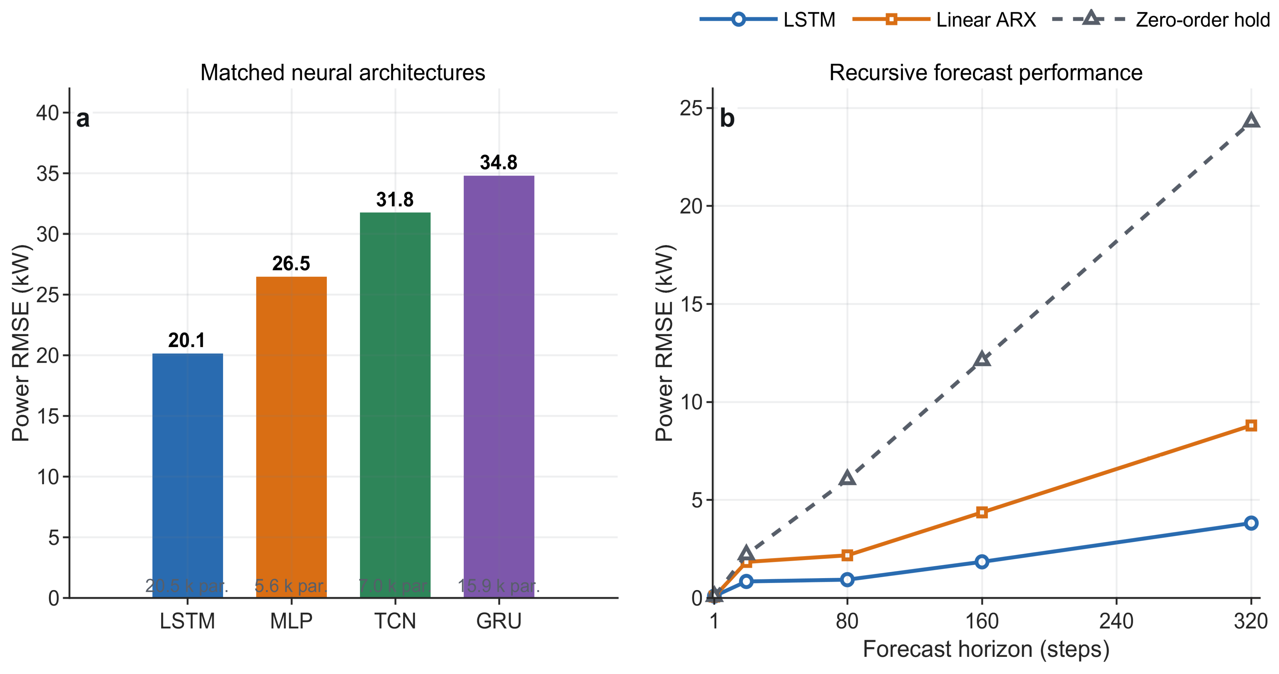
The matched neural comparison in Figure 4a gives power RMSE values of 20.15, 26.47, 31.76 and 34.79 kW for LSTM, MLP, TCN and GRU, respectively. LSTM uses 20,454 trainable parameters, compared with 15,910 for GRU, 7014 for TCN and 5622 for MLP. All four networks use the same case split, input and output channels, sampled training sequences and evaluation metrics. At one step, corrected LSTM RMSE is 0.099 kW, whereas linear ARX reaches 0.072 kW and zero-order hold prediction reaches 0.085 kW. At 20 steps the ordering reverses: LSTM gives 0.845 kW, ARX 1.841 kW and zero-order hold prediction 2.214 kW. At 320 steps the corresponding values are 3.822, 8.802 and 24.294 kW. The LSTM advantage is consequently a multi-step control horizon result, not a universal one-step claim.

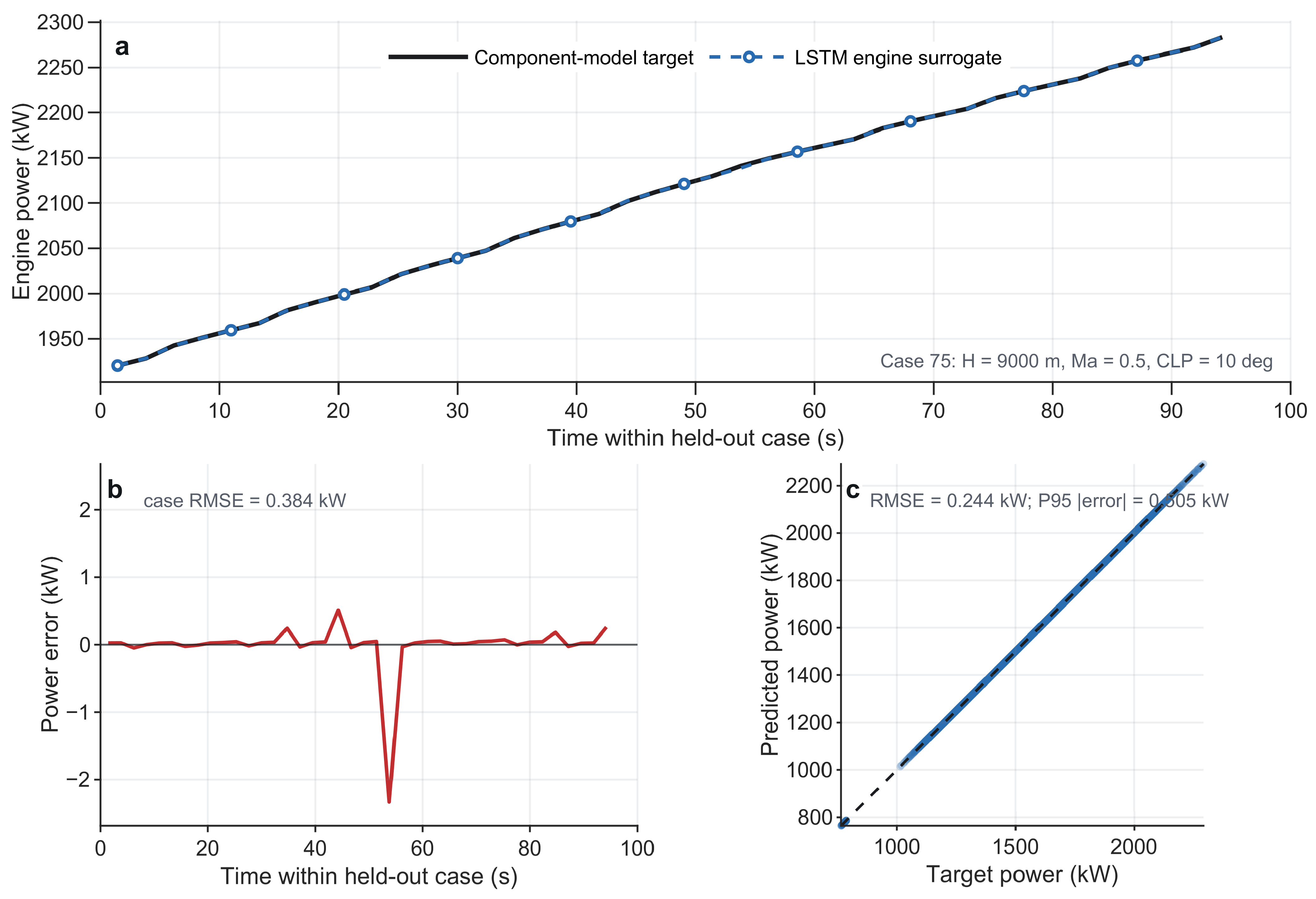
The final operational network uses all training cases at the selected capacity. Online correction reduces held-out power RMSE to 0.244 kW, with MAE 0.109 kW, a 95th-percentile absolute error of 0.505 kW and maximum error of 2.615 kW. The representative case in Figure 5 spans 363 kW and keeps the surrogate and component model power traces visually coincident; the residual panel and target prediction plot expose the remaining rare deviations rather than hiding them through axis scale. The 99th- and 99.9th-percentile power errors are 1.085 and 2.097 kW, respectively. Selected held-out power-prediction metrics are summarized in

Table 3. Selected power prediction results on held-out component model cases.

Model	Power Error (kW)	Definition
Matched LSTM	20.146	Architecture comparison before online correction
Matched MLP	26.473	Static time-window baseline
Matched TCN	31.755	Temporal convolution baseline
Matched GRU	34.790	Gated recurrent baseline
Operational LSTM	0.244	Held-out RMSE with online output correction
Operational LSTM	0.505	Held-out P95 absolute error
Operational LSTM	2.615	Held-out maximum absolute error
LSTM/ARX/zero-order hold	3.822/8.802/24.294	Power RMSE at 320 steps

.

5.2. Feature Attribution and Input Robustness

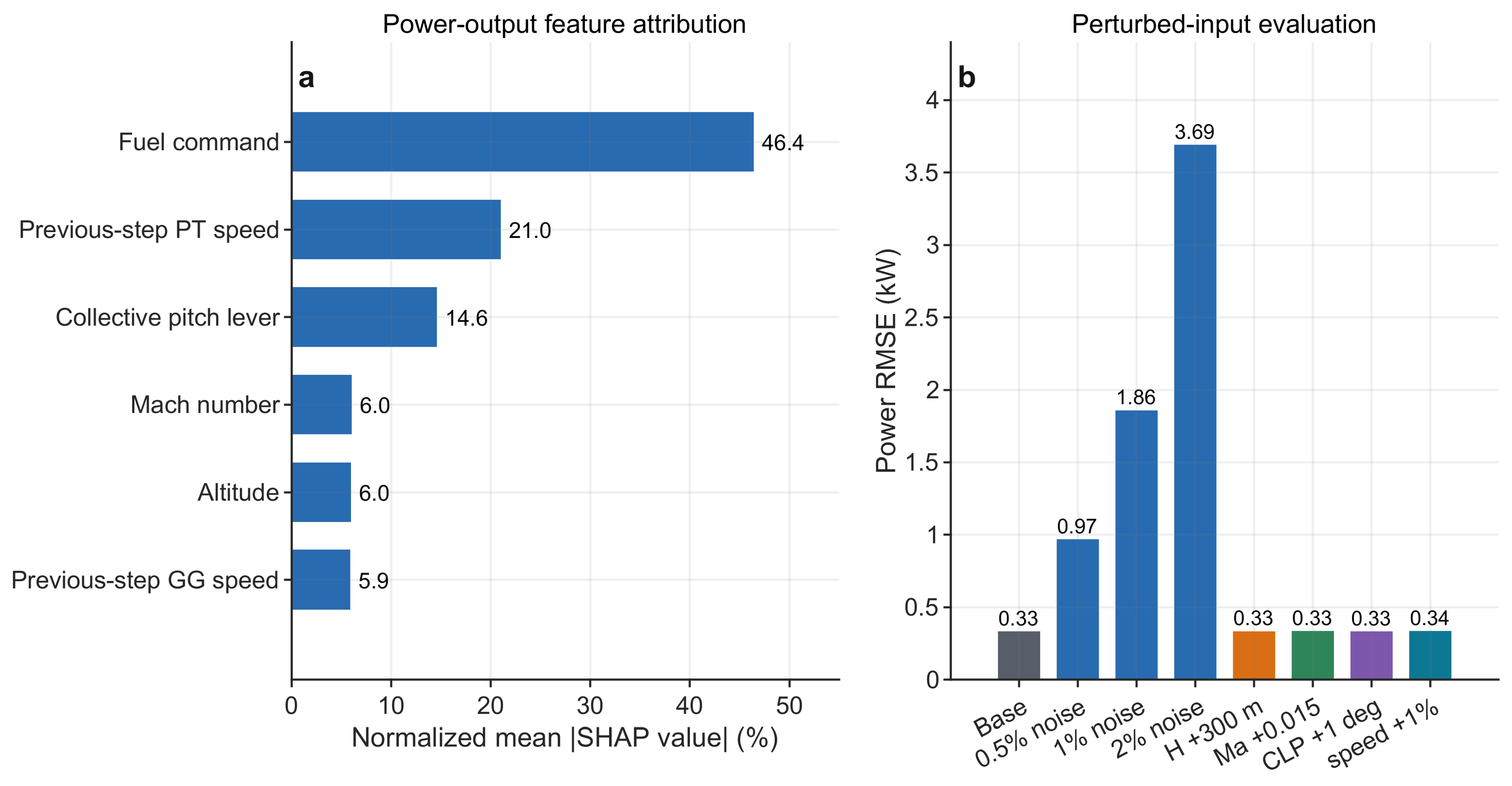
The SHAP feature importance analysis assigns 46.4% of the normalized mean absolute power attribution to the fuel command, 21.0% to previous-step power turbine speed and 14.6% to CLP. Mach, altitude and previous-step gas-generator speed contribute 6.0%, 6.0% and 5.9%, respectively. The result is physically plausible at the sampled operating points: fuel establishes the immediate energy input, while spool history carries inertial state. The values quantify model attribution rather than causal sensor importance, and correlated channels can exchange attribution.

Baseline power RMSE in the perturbation sample is 0.334 kW. Gaussian full-scale noise increases it to 0.968, 1.858 and 3.690 kW at 0.5%, 1% and 2%, respectively. The tested altitude, Mach, CLP and lag-gain biases change RMSE only modestly around the baseline, as summarized in Figure 6. This difference reflects the network’s stronger sensitivity to broadband sequence corruption than to the small constant offsets tested. It also identifies measurement filtering and uncertainty-aware training as higher priorities than claiming generic fault tolerance.

5.3. Conversion Flight Power Demand

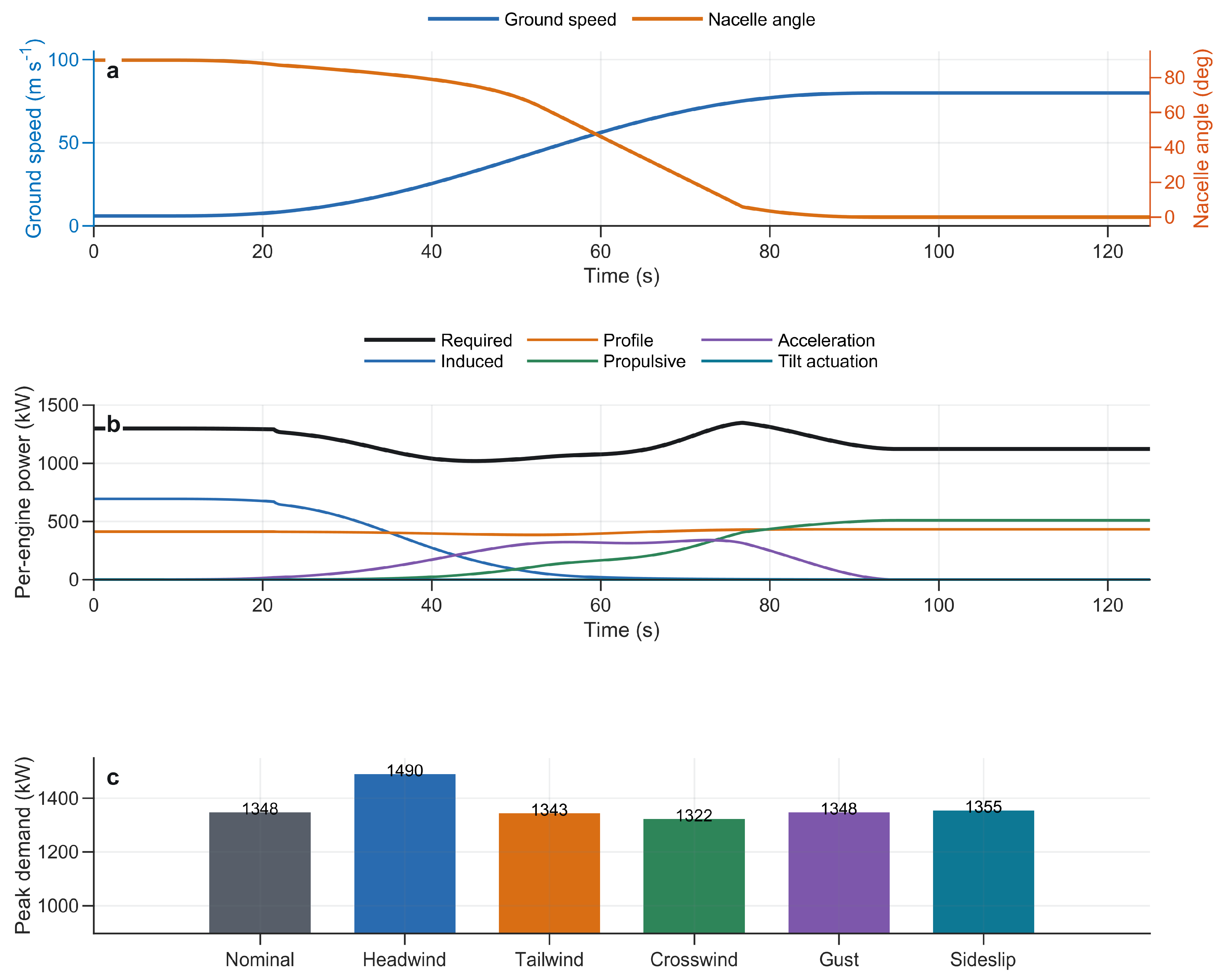
Figure 7 presents the conversion flight demand calculation. Speed rises from 6 to 80 m s⁻¹, while the actual nacelle angle, corrected by load balance and the tilt rate constraint, falls from 90 to 0 deg. As dynamic pressure builds, induced power decreases and propulsive power increases; profile power remains finite throughout because blade drag persists in every mode. Acceleration power peaks during the middle conversion interval, and nacelle actuation power is comparatively small. Total nominal per-engine demand ranges from 1019.0 to 1347.9 kW. A 10 m s⁻¹ headwind produces the largest peak, 1490.0 kW, whereas crosswind, gust and 5 deg sideslip cases peak at 1322.0, 1347.9 and 1354.7 kW, respectively. Every case remains inside the engine-data power range. The maximum tilt rate is 2.4 deg s⁻¹, the maximum rotor force direction error is 0.55 deg, and the worst blade-element thrust residual is 2.18 N.

These sensitivity cases partly address environmental variability but do not turn the two-dimensional model into a flight dynamic validation. Crosswind enters through resultant in-plane velocity and sideslip drag; it does not excite roll–yaw dynamics or differential rotor inflow. The gust is prescribed and deterministic. The numerical power spread should therefore be interpreted as a control-demand sensitivity envelope within the stated model, not as a probabilistic operational envelope.

5.4. Direct Component-Level Closed-Loop Control

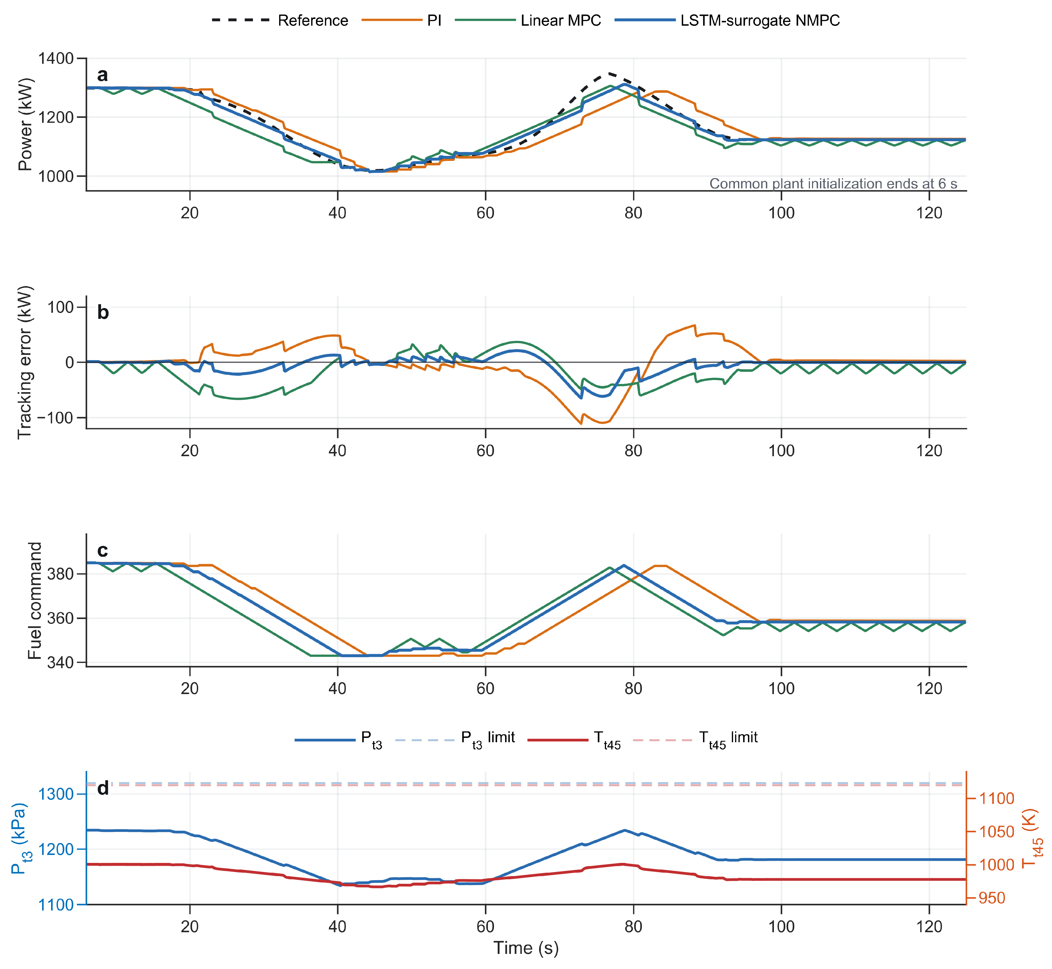
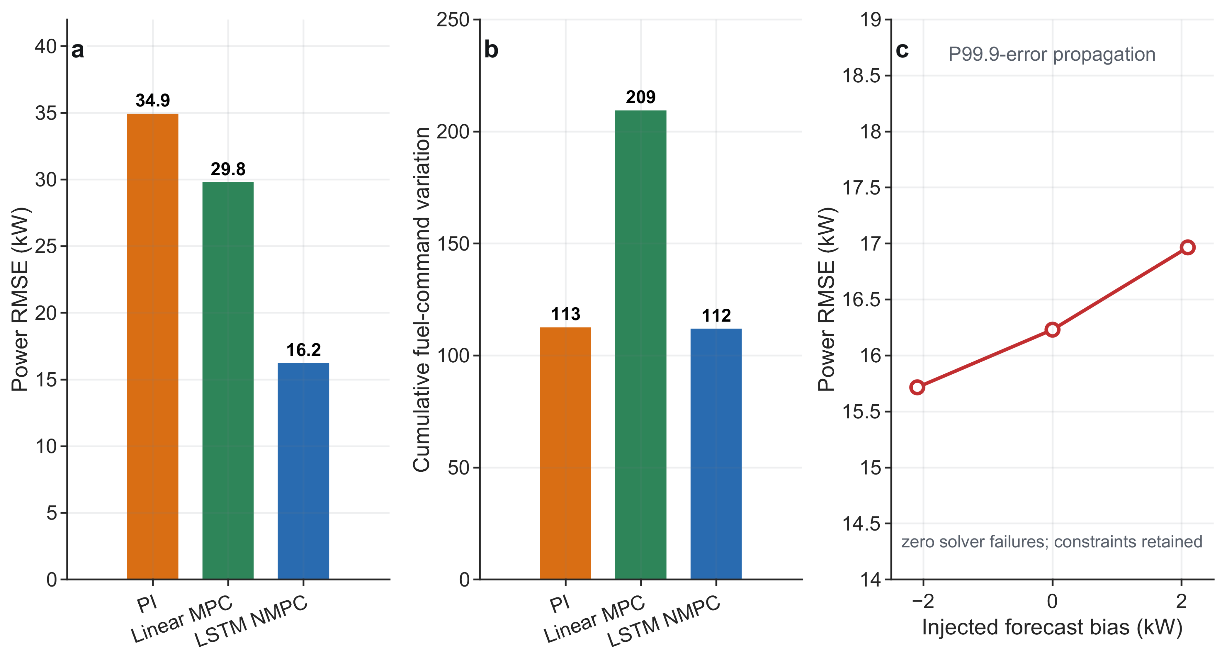
Figure 8 compares all controllers after the component-level engine reaches its initial steady state. PI control remains stable and non-oscillatory but reacts late to the broad demand trough and peak. Linear MPC aligns the peak most quickly yet develops a persistent negative tracking bias and uses a sawtooth fuel sequence after conversion. LSTM engine-surrogate NMPC reduces both the broad transient error and the late bias. The controller differences are distinct because the recurrent engine-surrogate, rather than a shared linear model, generates the LSTM controller’s future sensitivities.

The power RMSE is 34.94 kW for PI control, 29.80 kW for linear MPC and 16.23 kW for LSTM engine-surrogate NMPC. Relative to linear MPC, the recurrent controller improves the RMSE by 45.5% and the IAE by 61.5%; relative to PI control, the RMSE improves by 53.5%. Its maximum and 95th-percentile errors are 65.35 and 44.94 kW, respectively. The peak lag is 1.992 s, better than the PI controller’s 7.680 s but slower than linear MPC’s 0.072 s. Thus, the LSTM controller’s advantage lies in accumulated tracking and steady bias rather than fastest peak timing. Steady-state power error is −0.049 kW, compared with −9.843 kW for linear MPC and 2.574 kW for PI control.

All controllers reach the same hard fuel command rate limit of approximately 2 command units s⁻¹. LSTM engine-surrogate NMPC does not obtain lower error by allowing a larger peak rate: its cumulative fuel command variation is 111.98, close to the PI controller’s 112.57 and 46.5% below linear MPC’s 209.43. The maximum Tt45 and Pt3 are 1001.0 K and 1234.6 kPa, respectively, leaving margins of 119.0 K and 85.4 kPa to their prescribed limits. The mean and maximum solution times are 29.6 and 50.3 ms, respectively, both below the 1.92 s controller update interval, with no solver failures.

Injecting plus or minus 2.097 kW, the held-out 99.9th-percentile power error, changes closed-loop RMSE from 16.23 kW to 15.72 or 16.97 kW. The maximum tracking error remains below 67.5 kW, the fuel-rate constraint remains active, but unviolated, thermal and pressure constraints remain satisfied, and no optimizer failure occurs. Figure 9 summarizes these trade-offs. The experiment is a bounded bias-propagation test, not a complete reachability or adversarial-safety proof. The corresponding dynamic and computational control metrics are listed in

Table 4. Dynamic and computational control metrics for the component-level conversion experiment.

Controller	RMSE (kW)	IAE	Peak Lag (s)	Steady Error (kW)	Cumulative Fuel Variation	Max Rate	Mean Solve (ms)
PI	34.94	2634.35	7.680	2.574	112.57	2.000	0.04
Linear MPC	29.80	2800.35	0.072	−9.843	209.43	2.000	3.43
LSTM engine-surrogate NMPC	16.23	1078.27	1.992	−0.049	111.98	2.001	29.64

.

6. Discussion

The results indicate that the principal value of the LSTM-based engine-surrogate model lies in control-oriented multi-step prediction rather than universal superiority at every prediction horizon. The linear ARX model remained competitive for one-step prediction, whereas the corrected LSTM model achieved better accuracy over the longer horizons used by the predictive controller. This difference suggests that the recurrent model is particularly useful for representing the nonlinear and history-dependent engine response encountered during tiltrotor conversion flight. The aircraft model and the LSTM model perform distinct functions: the former calculates the future required shaft power from the conversion trajectory, whereas the latter predicts the engine response to operating conditions and fuel commands. Part of the multi-step improvement should also be attributed to online output correction rather than to the recurrent architecture alone.

The closed-loop results further show that higher prediction accuracy does not improve every control metric equally. Compared with linear MPC, the LSTM-assisted MPC reduced the overall power tracking error, integral error, steady-state deviation and cumulative fuel command variation, while linear MPC retained a slightly smaller peak response delay in some transients. This trade-off reflects the combined influence of prediction accuracy, controller weights, feedback correction and active constraints. Because all controllers were evaluated using the same fuel command magnitude and rate limits, the reduction in tracking error was not achieved by permitting more aggressive control action. The predicted turbine temperature and compressor-discharge pressure also remained within their prescribed limits. Nevertheless, the fuel command is expressed in model command units rather than a calibrated physical mass flow rate, so actuator feasibility cannot yet be inferred directly from these numerical results.

The numerical evidence supports the internal validity of the comparison within the investigated simulation framework. Complete operating cases were separated between training and testing, identical trajectories and constraints were applied to the competing controllers, and closed-loop performance was evaluated using the nonlinear component-level engine model rather than the surrogate model itself. However, the training data, test data and controlled plant were derived from the same component-level modelling framework and may therefore share component map assumptions and model-form errors. The exclusion of non-converged operating cases may also bias the dataset towards numerically feasible regions. Consequently, the demonstrated applicability is limited to interpolation within the sampled operating envelope and the prescribed conversion flight trajectories. The two-dimensional aerodynamic model does not reproduce full six-degree-of-freedom motion, dynamic stall, aeroelastic effects, detailed wake evolution or high-fidelity rotor–wing–nacelle interference. Moreover, the absence of independent rig or flight data prevents the results from being interpreted as experimental validation or evidence of flight readiness.

Further development should therefore focus on validation with independent engine-rig and flight-test data, followed by hardware-in-the-loop evaluation with calibrated fuel-metering, actuator and sensor dynamics. Coupling the controller to a six-degree-of-freedom aircraft model and higher-fidelity aerodynamic calculations would provide a more demanding assessment of conversion flight operation. Prediction uncertainty could also be quantified using ensemble or probabilistic recurrent models and incorporated into robust or stochastic MPC. These extensions would clarify the practical operating boundary of the approach and support its gradual transition from numerical demonstration to experimentally validated flight-propulsion control.

7. Conclusions

A blade-element/momentum-informed tiltrotor conversion model, an LSTM dynamic engine-surrogate and constrained predictive control were combined into a single numerical validation chain. The design comprised 537 converged component model cases with complete-case training, validation and held-out splits. LSTM produced the lowest power RMSE among matched LSTM, GRU, TCN and MLP baselines, and the corrected multi-step RMSE at 320 steps was 3.822 kW versus 8.802 kW for linear ARX and 24.294 kW for zero-order hold prediction. In a component-level closed loop, LSTM engine-surrogate NMPC achieved 16.23 kW power RMSE, compared with 29.80 kW for linear MPC and 34.94 kW for PI control. It reduced cumulative fuel command variation by 46.5% relative to linear MPC while respecting the same fuel command rate, temperature and pressure limits; the mean solution time was 29.6 ms for a 1.92 s update interval. These results support the LSTM as a control horizon engine-surrogate for the simulated conversion mission. Further validation requires actuator calibration, six-degree-of-freedom flight dynamics and independent rig or flight data.

References

- Maisel, M.D.; Giulianetti, D.J.; Dugan, D.C. The History of the XV-15 Tilt Rotor Research Aircraft: From Concept to Flight; SP-2000-4517; NASA Special Publication: Washington, DC, USA, 2000. Available online: https://www.nasa.gov/wp-content/uploads/2023/04/sp-4517.pdf (accessed on 8 September 2026).
- Sheng, H.; Zhang, C.; Xiang, Y. Mathematical Modeling and Stability Analysis of Tiltrotor Aircraft. Drones 2022, 6, 92. [Google Scholar] [CrossRef] [Scilit]
- Appleton, W.; Filippone, A.; Bojdo, N. Interaction Effects on the Conversion Corridor of Tiltrotor Aircraft. Aeronaut. J. 2021, 125, 2065–2086. [Google Scholar] [CrossRef] [Scilit]
- Su, W.; Qu, S.; Zhu, G.; Swei, S.S.-M.; Hashimoto, M.; Zeng, T. Modeling and Control of a Class of Urban Air Mobility Tiltrotor Aircraft. Aerosp. Sci. Technol. 2022, 124, 107561. [Google Scholar] [CrossRef] [Scilit]
- Yu, X.; Chen, R.; Wang, L.; Yan, X.; Yuan, Y. An Optimization for Alleviating Pilot Workload during Tilt Rotor Aircraft Conversion and Reconversion Maneuvers. Aerosp. Sci. Technol. 2022, 129, 107854. [Google Scholar] [CrossRef] [Scilit]
- Zhao, G.; Cui, Z.; Zhao, Q.; Chen, X.; Li, P. Investigations on Trimming Strategy and Unsteady Aerodynamic Characteristics of Tiltrotor in Conversion Procedure. Aerospace 2024, 11, 632. [Google Scholar] [CrossRef] [Scilit]
- Ruh, M.L.; Hwang, J.T. Robust Modeling and Optimal Design of Rotors Using Blade Element Momentum Theory. In Proceedings of the AIAA AVIATION 2021 Forum, AIAA 2021-2598, Virtual, 2–6 August 2021. [Google Scholar] [CrossRef] [Scilit]
- Li, S.; Wang, Y.; Zhang, H. Research on Adaptive Feedforward Control Method for Tiltrotor Aircraft/Turboshaft Engine System Based on Radial Basis Function Neural Network. Aerosp. Sci. Technol. 2024, 150, 109180. [Google Scholar] [CrossRef] [Scilit]
- Wang, Y.; Zheng, Q.; Zhang, H.; Chen, H. Research on Integrated Control Method for Helicopter/Turboshaft Engine with Variable Rotor Speed Based on the Error between Engine Required and Real Output Torque. Arab. J. Sci. Eng. 2020, 45, 6529–6540. [Google Scholar] [CrossRef] [Scilit]
- Song, J.; Wang, Y.; Ji, C.; Zhang, H. Real-Time Optimization Control of Variable Rotor Speed Based on Helicopter/Turboshaft Engine On-Board Composite System. Energy 2024, 301, 131701. [Google Scholar] [CrossRef] [Scilit]
- Wei, Z.; Zhang, S.; Jafari, S.; Nikolaidis, T. Gas Turbine Aero-Engines Real Time On-Board Modelling: A Review, Research Challenges, and Exploring the Future. Prog. Aerosp. Sci. 2020, 121, 100693. [Google Scholar] [CrossRef] [Scilit]
- Xu, M.; Liu, J.; Li, M.; Geng, J.; Wu, Y.; Song, Z. Improved Hybrid Modeling Method with Input and Output Self-Tuning for Gas Turbine Engine. Energy 2022, 238, 121672. [Google Scholar] [CrossRef] [Scilit]
- Paniccia, D.; Tucci, F.A.; Guerrero, J.; Capone, L.; Sanguini, N.; Benacchio, T.; Bottasso, L. A Supervised Machine-Learning Approach for Turboshaft Engine Dynamic Modeling under Real Flight Conditions. arXiv 2025, arXiv:2502.14120. [Google Scholar] [CrossRef] [Scilit]
- Garcia, C.E.; Prett, D.M.; Morari, M. Model Predictive Control: Theory and Practice—A Survey. Automatica 1989, 25, 335–348. [Google Scholar] [CrossRef] [Scilit]
- Mayne, D.Q.; Rawlings, J.B.; Rao, C.V.; Scokaert, P.O.M. Constrained Model Predictive Control: Stability and Optimality. Automatica 2000, 36, 789–814. [Google Scholar] [CrossRef] [Scilit]
- Qin, S.J.; Badgwell, T.A. A Survey of Industrial Model Predictive Control Technology. Control Eng. Pract. 2003, 11, 733–764. [Google Scholar] [CrossRef] [Scilit]
- Pang, S.W.; Li, Q.H.; Ni, B. Improved Nonlinear MPC for Aircraft Gas Turbine Engine Based on Semi-Alternative Optimization Strategy. Aerosp. Sci. Technol. 2021, 118, 106983. [Google Scholar] [CrossRef] [Scilit]
- Chen, Q.; Sheng, H.; Zhang, T. A Novel Direct Performance Adaptive Control of Aero-Engine Using Subspace-Based Improved Model Predictive Control. Aerosp. Sci. Technol. 2022, 128, 107760. [Google Scholar] [CrossRef] [Scilit]
- Wang, Y.; Zheng, Q.; Du, Z.; Zhang, H. Research on Nonlinear Model Predictive Control for Turboshaft Engines Based on Double Engines Torques Matching. Chin. J. Aeronaut. 2020, 33, 561–571. [Google Scholar] [CrossRef] [Scilit]
- Jung, M.; da Costa Mendes, P.R.; Önnheim, M.; Gustavsson, E. Model Predictive Control When Utilizing LSTM as Dynamic Models. Eng. Appl. Artif. Intell. 2023, 123, 106226. [Google Scholar] [CrossRef] [Scilit]
- Hochreiter, S.; Schmidhuber, J. Long Short-Term Memory. Neural Comput. 1997, 9, 1735–1780. [Google Scholar] [CrossRef] [Scilit]
- Gers, F.A.; Schmidhuber, J.; Cummins, F. Learning to Forget: Continual Prediction with LSTM. Neural Comput. 2000, 12, 2451–2471. [Google Scholar] [CrossRef] [Scilit]
- Greff, K.; Srivastava, R.K.; Koutnik, J.; Steunebrink, B.R.; Schmidhuber, J. LSTM: A Search Space Odyssey. IEEE Trans. Neural Netw. Learn. Syst. 2017, 28, 2222–2232. [Google Scholar] [CrossRef] [Scilit]
- Bengio, Y.; Simard, P.; Frasconi, P. Learning Long-Term Dependencies with Gradient Descent Is Difficult. IEEE Trans. Neural Netw. 1994, 5, 157–166. [Google Scholar] [CrossRef] [Scilit]
- Lundberg, S.M.; Lee, S.-I. A Unified Approach to Interpreting Model Predictions. Adv. Neural Inf. Process. Syst. 2017, 30, 4765–4774. Available online: https://proceedings.neurips.cc/paper_files/paper/2017/hash/8a20a8621978632d76c43dfd28b67767-Abstract.html (accessed on 8 September 2026).
- Song, J.; Wang, Y.; Li, S.; Zhang, H. Research on Incremental Nonlinear Dynamic Inverse Control Method for Turboshaft Engine Based on Jacobi Matrix. J. Low Freq. Noise Vib. Act. Control 2023, 42, 952–962. [Google Scholar] [CrossRef] [Scilit]
- Zhang, H.; Li, Y.; Deng, S. A Novel Emergent State Control Law for an Integrated Helicopter/Turboshaft Engine System. Math. Probl. Eng. 2014, 2014, 385807. [Google Scholar] [CrossRef] [Scilit]
- Wen, S.-X.; Zhang, Y.; Li, J.; Wang, K.; Liu, K.-Z.; Sun, X.-M. Thrust Estimation, Control, and Evaluation for Turbofan Engines. IEEE Trans. Aerosp. Electron. Syst. 2024, 60, 5186–5200. [Google Scholar] [CrossRef] [Scilit]
Figure 1.
Integrated conversion-flight and engine-control architecture. (a) Aircraft-side calculation from flight state and conversion aerodynamics to the horizon power reference. (b) Closed-loop signal path through the predictive optimizer, LSTM engine surrogate, fuel command and nonlinear component-level engine. Horizontal arrows denote forward signal flow; the upper-to-lower arrow supplies the aircraft-derived power reference, and the lower return arrow denotes measured engine feedback.
Figure 2.
Three-stage tiltrotor conversion and control-oriented aerodynamic model. (a) Helicopter, conversion and airplane modes. (b) Blade-relative velocity components, wing force balance, BEMT rotor solution, power aggregation, disturbance cases and the explicit two-dimensional model boundary.
Figure 3.
Numerical engine design and LSTM architecture. Panel (a): The complete-case training, validation and test assignment across CLP, altitude and Mach levels. Panel (b): The final engine-surrogate signal path and sequence length.
Figure 4.
Engine-predictor selection. Panel (a) compares power RMSE for matched LSTM, MLP, TCN and GRU models. Panel (b) compares corrected LSTM, linear ARX and zero-order hold prediction over the controller-relevant forecast horizon; linear ARX remains slightly better at one step.
Figure 5.
Held-out operational LSTM accuracy. Panel (a) shows a representative high-range component model case and LSTM prediction. Panel (b) exposes its power residual. Panel (c) shows all held-out target prediction pairs with the equality line.
Figure 6.
Engine-surrogate interpretation and perturbed-input evaluation. Panel (a) reports normalized mean absolute SHAP attribution for the power output. Panel (b) reports power RMSE under representative sequence noise and constant sensor-channel biases.
Figure 7.
Tiltrotor conversion demand experiment. Panel (a) gives speed and coordinated nacelle angle. Panel (b) decomposes blade-derived per-engine demand into induced, profile, propulsive, acceleration and tilt actuation contributions. Panel (c) compares peak demand under wind, gust and sideslip cases.
Figure 8.
Direct nonlinear component-level closed-loop comparison after the engine reaches its initial steady state. (a) Required and delivered shaft power. (b) Power-tracking error. (c) Fuel command. (d) Compressor-discharge total pressure and turbine temperature predicted for the LSTM engine-surrogate NMPC case, together with their limits. All controllers use the same conversion demand, trim schedule and hard fuel constraints.
Figure 9.
Closed-loop metrics and rare-error propagation. (a) Power RMSE for the three controllers. (b) Cumulative fuel-command variation. (c) Closed-loop effect of injecting the positive and negative 99.9th-percentile LSTM power error across the prediction horizon.