Fault-Tolerant Attitude Control of Flexible Spacecraft via Reinforcement Learning

Abstract

This paper proposes an integrated attitude control framework for flexible spacecraft subject to external disturbances, rigid–flexible dynamic coupling, and actuator faults. The control framework combines the Twin Delayed Deep Deterministic Policy Gradient (TD3) reinforcement learning algorithm with an adaptive fault-tolerant (AFT) compensator. First, a rigid–flexible coupling dynamic model is formulated using Modified Rodrigues Parameters. Second, an observer-based TD3 attitude controller is designed, where a hierarchical reward function incorporating the observer-estimated flexible modal displacement $\widehat{\mathit{\eta }}$ is constructed to train the agent for simultaneous attitude convergence and vibration suppression. Third, a composite fault-tolerant control structure is developed by integrating the trained TD3 policy with an adaptive sliding mode compensator that handles both partial loss-of-effectiveness faults and time-varying additive faults. The proposed framework is evaluated under a progressive five-scenario uncertainty evaluation framework encompassing measurement noise, parameter mismatch, external disturbances, and actuator faults. Simulation results demonstrate that (i) the $\widehat{\mathit{\eta }}$-augmented reward enables substantial improvements in vibration suppression over the baseline reward, achieving a better balance between pointing accuracy and vibration attenuation; (ii) under the most demanding fault scenario, the AFT compensator proves essential for precise convergence, and the composite TD3+AFT architecture achieves the best overall performance among the four compared control schemes.

1. Introduction

Flexible spacecraft attitude control represents a critical yet challenging problem in modern space missions, characterized by rigid–flexible coupling effects, multi-source uncertainties, and stringent performance requirements [1,2]. Unlike rigid spacecraft, flexible spacecraft feature large lightweight appendages (such as solar arrays and antenna reflectors) that introduce low-frequency elastic vibrations intrinsically coupled with rigid-body attitude motion, degrading pointing accuracy and risking persistent oscillations during maneuvers [2].

Recent advances have addressed flexible vibration suppression, disturbance rejection, actuator fault tolerance, and agile maneuvering through disturbance observers, sliding mode control (SMC), input shaping, and prescribed performance control. Observer-based and SMC approaches include Golestani et al.’s fixed-time disturbance observer with prescribed performance control [1], Shahid et al.’s composite anti-unwinding finite-time adaptive sliding mode with a modal vibration observer [3], and Dian et al.’s scheduled input shaping with sinusoidal path planning and a nonlinear disturbance observer [4]. For synchronous maneuver and vibration suppression, He and Cao designed cooperative linear quadratic regulator (LQR) and proportional-derivative (PD) with input shaping [2], Zhong et al. employed the internal model principle to asymptotically reject sinusoidal disturbances without modal measurements [5], and Song and Agrawal experimentally validated pulse width pulse frequency (PWPF) modulation with positive position feedback to attenuate thruster-induced vibrations [6]. Robust and adaptive approaches addressing model uncertainties include Yu et al.’s gain-scheduled $H_{\infty }$ control for large-angle maneuvers [7], Angeletti et al.’s end-to-end robust design via linear fractional transformation [8], and Khoroshylov et al.’s adaptive notch-filter strategies for space-based synthetic aperture radar (SAR) platforms [9].

Deep reinforcement learning (DRL) has emerged as a broader trend in spacecraft guidance, navigation, and control, as surveyed in recent reviews [10,11,12]. Among DRL algorithms, the Twin Delayed Deep Deterministic policy gradient (TD3) [13] is selected in this work for its deterministic policy formulation well-suited for continuous torque commands, off-policy sample efficiency critical for computationally expensive flexible-body simulations, and twin-critic architecture that mitigates value overestimation bias. TD3 has been extensively applied across aerospace scenarios including unmanned aerial vehicle (UAV) operations [14,15,16,17,18], spacecraft attitude control [19], hypersonic vehicle maneuvering [20], and aero-engine regulation [21], with algorithmic modifications such as proportional-integral-derivative (PID)-guided exploration [19], Steffensen value iteration (SVI) for faster convergence [22], frame stacking for energy-efficient UAV path planning [14], and 3D environment encoding for dynamic obstacle avoidance [16].

More recently, several works have explored the intersection of TD3/DRL with flexible spacecraft dynamics and fault-tolerant control. Shi et al. [23] applied TD3 to cooperative control of ultra-close flexible spacecraft formation flying. Li et al. [24] integrated a DRL-based disturbance observer with the fully-actuated system approach for dumbbell-shaped flexible spacecraft. In the direction of fault tolerance, El-Dalahmeh et al. [25] developed TD3-HD with Hindsight Experience Replay for attitude fault recovery, and Henna et al. [26] introduced expert-guided exploration for satellite fault-tolerant attitude control. Nevertheless, two gaps remain to be addressed. First, Shi et al. [23] and Li et al. [24] address flexible attitude control without considering actuator faults. Second, El-Dalahmeh et al. [25] and Henna et al. [26] address fault-tolerant control but treat the spacecraft as rigid, neglecting rigid–flexible coupling dynamics. To the best of the authors’ knowledge, no existing work has simultaneously addressed flexible vibration suppression and actuator fault tolerance within a unified TD3-based framework.

Motivated by this gap, this paper develops an integrated attitude control framework for flexible spacecraft stabilization, capable of simultaneously addressing external disturbances, rigid–flexible coupling dynamics, and actuator faults. The framework employs the TD3 algorithm integrated with adaptive fault-tolerant control.The main contributions of this work are: (1) A hierarchical phased reward function for TD3-based flexible spacecraft attitude control. Unlike prior reward designs that rely solely on attitude error [27] or lack vibration-aware shaping [23,24], the proposed reward comprises four components (base, convergence, smoothness, and terminal) implementing a phased convergence strategy, with the convergence term augmented by observer-estimated flexible modal displacement $\widehat{\mathit{\eta }}$ to explicitly guide oscillation suppression. (2) A composite fault-tolerant control structure integrating the trained TD3 agent with an adaptive sliding mode fault-tolerant (AFT) compensator, extending the integral-type sliding mode framework of [28] from rigid to flexible spacecraft. The sliding manifold and AFT compensator are reformulated with rigid–flexible coupling terms (${\mathit{\delta }}^T\ddot{\mathit{\eta }}$ and ${\mathit{\delta }}^T\dot{\mathit{\eta }}$) using observer-estimated modal coordinates.

The source code and simulation scripts accompanying this work are openly available at https://github.com/EllencePeng/Aerospace-RL-Flexible-Spacecraft (accessed on 18 June 2026).

The organization of this paper is as follows: Section 1 presents the research background and motivation. Section 2 presents the flexible spacecraft dynamics, fault model, flexible state observer, and problem statement. Section 3 establishes the RL training framework. Section 4 designs the adaptive fault-tolerant controller. Section 5 verifies the proposed schemes via simulations. Section 6 concludes this paper by summarizing its main contributions and putting forward prospects for future research.

2. Preliminaries

2.1. Flexible Spacecraft Attitude Dynamics and Kinematics

Two reference frames are used throughout this paper: an inertial reference frame $\mathcal{I}$ and a body-fixed frame $\mathcal{B}$ attached to the spacecraft’s main body. The angular velocity vector $\mathit{\omega }\in {\mathbb{R}}^3$ represents the inertial angular velocity of the spacecraft with respect to $\mathcal{I}$ and expressed in $\mathcal{B}$. The attitude orientation of $\mathcal{B}$ with respect to $\mathcal{I}$ is described by the Modified Rodrigues Parameters (MRPs) [29], denoted by $\mathit{p}\in {\mathbb{R}}^3$. The corresponding attitude kinematic model, derived by referring to the modeling method in [30], is given by

$$\dot{\mathit{p}}={\displaystyle \frac{1}{4}}\left[\left(1-{\mathit{p}}^T\mathit{p}\right){\mathit{I}}_3+2{\mathit{p}}^{\times }+2\mathit{p}{\mathit{p}}^T\right]\mathit{\omega }=\mathit{T}\left(\mathit{p}\right)\mathit{\omega },$$

(1)

where $\mathit{p}\in {\mathbb{R}}^3$ represents the MRP vector, and ${\mathit{I}}_3$ denotes the $3\times 3$ identity matrix. The compact form $\mathit{T}\left(\mathit{p}\right)\mathit{\omega }$ is adopted for brevity in subsequent equations. The symbol ${\mathit{p}}^{\times }$ denotes the skew-symmetric matrix of $\mathit{p}$, defined as

$${\mathit{p}}^{\times }=\left[\begin{array}{ccc}0& -p_3& p_2\\ p_3& 0& -p_1\\ -p_2& p_1& 0\end{array}\right].$$

(2)

Compared with conventional attitude parameterizations, MRPs provide a computationally efficient and numerically robust attitude description [29], well-suited for precise spacecraft attitude control simulation. MRPs are globally valid for eigenaxis rotations up to 360°, but encounter a singularity where $\parallel \mathit{p}\parallel \to \infty$ when the rotation angle reaches exactly 360°. This is readily handled by shadow-set switching. Since all maneuvers considered in this work involve rotation angles far below 360°, $\parallel \mathit{p}\parallel$ remains well within the unit sphere and shadow-set switching is unnecessary here.

The attitude dynamics of flexible spacecraft is adopted from [31] in low Earth orbit (LEO), formulated as

$$\left\{\begin{array}{c}\mathit{J}\dot{\mathit{\omega }}+{\mathit{\delta }}^T\ddot{\mathit{\eta }}=-{\mathit{\omega }}^{\times }\left(\mathit{J}\mathit{\omega }+{\mathit{\delta }}^T\dot{\mathit{\eta }}\right)+\mathit{\tau }\hfill \\ \ddot{\mathit{\eta }}+\mathit{C}\dot{\mathit{\eta }}+\mathit{K}\mathit{\eta }=-\mathit{\delta }\dot{\mathit{\omega }}\hfill \end{array}\right.,$$

(3)

where $\mathit{J}\in {\mathbb{R}}^{3\times 3}$ denotes the inertial matrix of the spacecraft, $\mathit{\tau }\in {\mathbb{R}}^3$ is the control torque input, $\mathit{\delta }$ represents the coupling matrix between the rigid main body and flexible appendages, and $\mathit{\eta }\in {\mathbb{R}}^m$ denotes the flexible modal coordinates vector, treated as dimensionless. m is the total number of flexible vibration modes, $\mathit{C}=\mathrm{diag}\{2{\xi }_i{\omega }_{n_i},i=1,\dots ,m\}$ and $\mathit{K}=\mathrm{diag}\{{\omega }_{n_i}^2,i=1,\dots ,m\}$ are the modal damping and stiffness matrices respectively, ${\omega }_{n_i}$ is the natural frequency of the i-th flexible mode, and ${\xi }_i$ is the corresponding damping ratio.

2.2. Fault Model

Assume that the dynamic response characteristics of spacecraft actuators can be ignored. An actuator is defined as fault-free when its output signal is completely consistent with the input command. The typical actuator faults considered in this study are modeled based on the existing research framework as follows [28]:

$$\mathit{\tau }=\left[{\mathit{I}}_3-\mathit{E}\left(t\right)\right]\mathit{u}+\overline{\mathit{u}},$$

(4)

where $\mathit{E}\left(t\right)=\mathrm{diag}\{e_1\left(t\right),e_2\left(t\right),e_3\left(t\right)\}\in {\mathbb{R}}^{3\times 3}$ represents the actuator efficiency loss matrix of the spacecraft, satisfying $0\le e_i\left(t\right)<1(i=1,2,3)$. Specifically, the condition $e_i\left(t\right)=0$ means the $i_{\mathrm{th}}$ actuator operates in a normal state, while $0<e_i\left(t\right)<1$ indicates the $i_{\mathrm{th}}$ actuator suffers from partial efficiency loss without complete functional failure. Additionally, $\overline{\mathit{u}}\in {\mathbb{R}}^3$ denotes the bounded time-varying additive fault occurring in the actuator. On this basis, the nonlinear attitude dynamic model of the spacecraft, which integrates the actuator fault model (4) and external disturbance $\mathit{d}$, can be reconstructed as the following expression:

$$\mathit{J}\dot{\mathit{\omega }}+{\mathit{\delta }}^T\ddot{\mathit{\eta }}=-{\mathit{\omega }}^{\times }\left(\mathit{J}\mathit{\omega }+{\mathit{\delta }}^T\dot{\mathit{\eta }}\right)+\left[{\mathit{I}}_3-\mathit{E}\left(t\right)\right]\mathit{u}+\overline{\mathit{u}}+\mathit{d}.$$

(5)

To lay a solid foundation for the design of the composite fault-tolerant controller, three reasonable assumptions are proposed for the actuator faults and external disturbances, as detailed below.

Assumption 1.

The external disturbance $\mathit{d}$ is bounded, satisfying $∥\mathit{d}∥\le d_m$, where $d_m$ is a positive scalar and $∥·∥$ represents the Euclidean norm.

Assumption 2.

For the actuator efficiency loss matrix $\mathit{E}\left(t\right)=\mathrm{diag}\{e_1\left(t\right),e_2\left(t\right),e_3\left(t\right)\}$, the inequality $0\le \max \{e_1,e_2,e_3\}\le e_m<1$ holds, where $e_m$ is a positive scalar.

Assumption 3.

The time-varying additive actuator fault $\overline{\mathit{u}}$ is bounded, satisfying $∥\overline{\mathit{u}}∥\le {\overline{u}}_m$, with ${\overline{u}}_m$ being a positive constant.

Remark 1.

Assumptions 1–3 are consistent with the actual operating environment of most spacecraft systems. Assumption 1 states that the external disturbance $\mathit{d}$ acting on the flexible spacecraft is norm-bounded, which is consistent with the fact that environmental perturbations (atmospheric drag, gravity gradient, and solar radiation pressure) are always limited in actual space missions. Assumption 2 describes the actuator partial loss of effectiveness fault, where the upper bound $0\le e_m<1$ ensures that the actuator still retains a certain control ability rather than complete failure. Assumption 3 restricts the additive actuator fault to be bounded, reflecting that the deviation or bias caused by component aging, signal drift or mechanical wear is always finite in real physical systems. These physically meaningful assumptions provide a practical prerequisite for the design and analysis of the fault-tolerant control scheme.

2.3. Flexible State Observer

In practice, the flexible modal variables $\mathit{\eta }$ and $\dot{\mathit{\eta }}$ are not directly measurable by onboard sensors. To address this, the nonlinear observer developed by Zou et al. [30] is adopted. The observer is of the high-gain type: it exploits the rigid–flexible coupling through the matrix $\mathit{\delta }$ to infer the unmeasurable modal states from the available attitude measurement $\mathit{p}$. The correction terms $\theta {\theta }_1\tilde{\mathit{p}}$ and ${\theta }^2{\theta }_2\tilde{\mathit{p}}$, driven by the attitude estimation error $\tilde{\mathit{p}}=\mathit{p}-\widehat{\mathit{p}}$, propagate through the coupled dynamics to update the estimates of $\widehat{\mathit{v}}$, $\widehat{\mathit{\eta }}$, and $\widehat{\mathit{\psi }}$. A single design parameter $\theta >0$ governs the convergence rate; by choosing a sufficiently large $\theta$, the estimation errors $(\tilde{\mathit{p}},\tilde{\mathit{v}},\tilde{\mathit{\eta }},\tilde{\mathit{\psi }})$ are guaranteed to converge to zero exponentially. The complete observer dynamics are given by

$$\left\{\begin{array}{c}\dot{\widehat{\mathit{p}}}=\widehat{\mathit{v}}+\theta {\theta }_1\tilde{\mathit{p}},\hfill \\ \dot{\widehat{\mathit{v}}}=f(\mathit{p},\widehat{\mathit{v}},\widehat{\mathit{\eta }},\widehat{\mathit{\psi }})+g\mathit{\tau }+{\theta }^2{\theta }_2\tilde{\mathit{p}},\hfill \\ \dot{\widehat{\mathit{\eta }}}=\widehat{\mathit{\psi }}-\mathit{\delta }\mathit{P}\widehat{\mathit{v}},\hfill \\ \dot{\widehat{\mathit{\psi }}}=-\mathit{C}\widehat{\mathit{\psi }}-\mathit{K}\widehat{\mathit{\eta }}+\mathit{C}\mathit{\delta }\mathit{P}\widehat{\mathit{v}},\hfill \end{array}\right.$$

(6)

where $\mathit{v}=\dot{\mathit{p}}$, $\mathit{\psi }=\dot{\mathit{\eta }}+\mathit{\delta }\mathit{\omega }$, $\mathit{P}={\mathit{T}}^{-1}$, $g=\mathit{T}{\overline{\mathit{J}}}^{-1}$, $\overline{\mathit{J}}=\mathit{J}-{\mathit{\delta }}^T\mathit{\delta }$ and $f(\mathit{p},\mathit{v},\mathit{\eta },\mathit{\psi })=-\mathit{T}\dot{\mathit{P}}\mathit{v}-\mathit{T}{\overline{\mathit{J}}}^{-1}{\left(\mathit{P}\mathit{v}\right)}^{\times }\left(\overline{\mathit{J}}\mathit{P}\mathit{v}+{\mathit{\delta }}^T\mathit{\psi }\right)+\mathit{T}{\overline{\mathit{J}}}^{-1}{\mathit{\delta }}^T\left(\mathit{C}\mathit{\psi }+\mathit{K}\mathit{\eta }-\mathit{C}\mathit{\delta }\mathit{P}\mathit{v}\right)$. $\theta$, ${\theta }_1$ and ${\theta }_2$ are positive constants, $\widehat{\mathit{p}}$ with $\widehat{\mathit{p}}\left(0\right)=\mathit{p}\left(0\right)$ and $\widehat{\mathit{v}}$ with $\widehat{\mathit{v}}\left(0\right)=0$ are estimates of $\mathit{p}$ and $\mathit{v}$, respectively, $\tilde{\mathit{p}}=\mathit{p}-\widehat{\mathit{p}}$ and $\widehat{\mathit{\psi }}$, $\widehat{\mathit{\eta }}$ are estimates of $\mathit{\psi }$, $\mathit{\eta }$. The observer gains in this work are set as $\theta =5.0$, ${\theta }_1=2.0$, and ${\theta }_2=5.0$.

2.4. Problem Statement

Problem 1.

For a flexible spacecraft system modeled in as (1) and (3), under concurrent external disturbances and actuator faults described by (4), design a composite control scheme combining reinforcement learning and adaptive fault-tolerant control to achieve attitude stabilization and vibration suppression.

3. TD3-Based Controller Design

This section formulates a baseline controller utilizing the TD3 algorithm for flexible spacecraft attitude stabilization under fault-free conditions. The TD3 algorithm is first briefly reviewed, followed by three design aspects that instantiate it for the problem at hand: the state and action representation, the reward function, and the network architectures.

3.1. TD3 Algorithm

TD3 is an off-policy actor–critic algorithm for continuous control, proposed by Fujimoto et al. [13] as an improvement over DDPG. It employs twin critic networks and delayed policy updates to mitigate value overestimation, and a deterministic policy that is well-suited for generating smooth continuous torque commands. The training procedure follows the standard TD3 protocol established in [13].

3.2. State and Action Representation

It is assumed that only the attitude and angular velocity of the flexible spacecraft are directly measurable, while the flexible modal displacement $\mathit{\eta }$ is not directly measurable but can be estimated by the observer introduced in Section 2.3. Consequently, flexible modal coordinates are excluded from the state vector provided to the TD3 policy.

The state vector provided to the TD3 policy is defined as

$${\mathit{s}}_{RL}={\left[\begin{array}{cc}{\mathit{p}}^T& {\mathit{\omega }}^T\end{array}\right]}^T\in {\mathbb{R}}^6,$$

(7)

The action generated by the policy corresponds to the continuous control torque applied to the spacecraft body. The action vector is defined as

$$\mathit{a}=\mathit{\tau }\in {\mathbb{R}}^3,$$

(8)

where $\mathit{\tau }$ represents the control torque along the three principal body axes.

To ensure actuator feasibility, the control torque is subjected to saturation constraints,

$$\parallel \mathit{\tau }\parallel \le u_{\max },$$

(9)

where $u_{\max }=1$ N·m denotes the maximum allowable actuator torque, a value consistent with the torque capacity of reaction wheels typically employed on small-to-medium-class spacecraft.

3.3. Reward Function Design

The reward function implements a phased convergence strategy with four components:

$$R=R_{\mathrm{base}}+R_{\mathrm{convergence}}+R_{\mathrm{smoothness}}+R_{\mathrm{terminal}}$$

(10)

where the 1-norm of $\mathit{p}$ is defined as ${\parallel \mathit{p}\parallel }_1=|p_1|+|p_2|+|p_3|$.

The base reward provides dense per-step signals during the large-error phase (${\parallel \mathit{p}\parallel }_1\ge 0.5$):

$$R_{\mathrm{base}}=\left\{\begin{array}{cc}1-{\parallel \mathit{\tau }\parallel }^2,\hfill & {\mathrm{if}\parallel \mathit{p}\parallel }_1\ge {0.5\mathrm{and}(\parallel \mathit{p}\parallel }_1<\parallel {\mathit{p}}_{\mathrm{prev}}{\parallel }_1)\hfill \\ 1-{\parallel \mathit{\tau }\parallel }^2,\hfill & {\mathrm{if}\parallel \mathit{p}\parallel }_1\ge {0.5\mathrm{and}(\parallel \mathit{\omega }\parallel }_1<\parallel {\mathit{\omega }}_{\mathrm{prev}}{\parallel }_1)\hfill \\ -{\parallel \mathit{p}\parallel }_1-{10\parallel \mathit{\omega }\parallel }_1-{\parallel \mathit{\tau }\parallel }^2,\hfill & \mathrm{otherwise}\hfill \end{array}\right.$$

(11)

The piecewise monotonic-improvement condition rewards the agent with $1-{\parallel \mathit{\tau }\parallel }^2$ when the attitude or angular velocity error decreases, and penalizes all error sources otherwise. The coefficient 10 on ${\parallel \mathit{\omega }\parallel }_1$ normalizes it to the scale of ${\parallel \mathit{p}\parallel }_1$.

When ${\parallel \mathit{p}\parallel }_1<0.5$, inverse-proportional rewards are activated to accelerate fine convergence:

$$R_{\mathrm{convergence},1}=\left\{\begin{array}{cc}{\displaystyle \frac{1}{{\parallel \mathit{p}\parallel }_1+0.01}}+{\displaystyle \frac{0.05}{{\parallel \mathit{\omega }\parallel }_1+0.01}},\hfill & {\parallel \mathit{p}\parallel }_1<0.5\hfill \\ 0,\hfill & \mathrm{otherwise}\hfill \end{array}\right.$$

(12)

The form $1/(\parallel \mathit{p}{\parallel }_1+0.01)$ is chosen because its gradient steepens as the error shrinks, naturally accelerating fine convergence. The $+0.01$ offset prevents division by zero and caps the reward, avoiding destabilizing Q-value targets during critic training.

To explicitly suppress flexible vibrations, the observer-estimated modal displacement $\widehat{\mathit{\eta }}$ (Section 2.3) is incorporated into the convergence reward:

$$R_{\mathrm{convergence},2}=\left\{\begin{array}{cc}{\displaystyle \frac{1}{{\parallel \mathit{p}\parallel }_1+0.01}}+{\displaystyle \frac{0.05}{{\parallel \mathit{\omega }\parallel }_1+0.01}}+{\displaystyle \frac{0.05}{\parallel \widehat{\mathit{\eta }}{\parallel }_2+0.01}},\hfill & {\parallel \mathit{p}\parallel }_1<0.5\hfill \\ 0,\hfill & \mathrm{otherwise}\hfill \end{array}\right.$$

(13)

The additional term uses the same inverse-proportional form. The weight $0.05$ (vs. $1.0$ for attitude) encodes a 20:1 priority ratio, reflecting that vibration suppression is subordinate to attitude convergence. The agents trained with these two formulations—agent $A_0$ (without $\widehat{\mathit{\eta }}$) and agent A (with $\widehat{\mathit{\eta }}$)—are compared in Section 5.3.

Smoothness penalties discourage abrupt actuation:

$$R_{\mathrm{smoothness}}=-10·{\parallel \mathit{\tau }-{\mathit{\tau }}_{\mathrm{prev}}\parallel }_1+\left\{\begin{array}{cc}-10·{\parallel \mathit{\tau }\parallel }^2,\hfill & {\parallel \mathit{p}\parallel }_1<0.01\hfill \\ 0,\hfill & \mathrm{otherwise}\hfill \end{array}\right.$$

(14)

where ${\mathit{\tau }}_{\mathrm{prev}}$ denotes the RL output at the previous timestep. The L1-norm penalizes torque chattering linearly without being dominated by occasional large transients; the quadratic penalty $-{\parallel \mathit{\tau }\parallel }^2$ activates only near convergence to prevent wasteful energy expenditure.

Upon termination, a graduated reward is assigned based on final convergence precision:

$$R_{\mathrm{terminal}}=\left\{\begin{array}{cc}-100,\hfill & {\parallel \mathit{p}\parallel }_{\infty }\ge 1\mathrm{or}{\parallel \mathit{\omega }\parallel }_{\infty }\ge 1\mathrm{rad}/\mathrm{s}\hfill \\ 1000,\hfill & {\parallel \mathit{p}\parallel }_1<0.01\hfill \\ 200,\hfill & 0.01\le {\parallel \mathit{p}\parallel }_1<0.05\hfill \\ 100,\hfill & 0.05\le {\parallel \mathit{p}\parallel }_1<0.1\hfill \\ 0,\hfill & \mathrm{otherwise}\hfill \end{array}\right.$$

(15)

where ${\parallel \mathit{p}\parallel }_{\infty }=\max \left(\right|p_1|,|p_2|,|p_3\left|\right)$. The graduated tiers ($+1000$, $+200$, $+100$) provide a curriculum-like signal: partial credit during early training helps the agent discover the basin of attraction, while progressively tighter thresholds refine convergence as the policy improves. The $-100$ divergence penalty supplements the opportunity cost of forfeited future rewards.

All weights and thresholds are calibrated so that each component’s magnitude remains comparable at its intended phase.

3.4. Network Structures

Both the actor and critic networks follow the standard TD3 architecture of Fujimoto et al. [13], employing two hidden layers with 400 and 300 units, respectively. The network structures are summarized in

Table 1. Network architectures of the actor and critic.

Component	Architecture	Activation
Actor	$6\to 400\to 300\to 3$	ReLU (hidden), tanh (output)
Critic	$9\to 400\to 300\to 1$	ReLU (hidden), linear (output)

.

The actor output is passed through a tanh activation scaled by $u_{\max }$ to respect the saturation limits defined in Section 3.2. The critic concatenates the state and action at its input layer and outputs a scalar Q-value. All hidden layers use ReLU activations; no batch normalization or dropout is applied.

4. Fault-Tolerant Attitude Controller Design

While the reinforcement learning-based controller offers significant advantages in adaptability and reduces manual tuning, its limitations in handling specific actuator fault modes necessitate the development of a dedicated fault-tolerant control scheme. Building upon the integral-type sliding mode framework of [28], an adaptive fault-tolerant (AFT) controller is formulated in this section. The proposed composite structure extends the framework of [28] in two key aspects: (i) the nominal controller is replaced by the trained TD3 agent rather than the saturated PD law in [28], which was designed for rigid-body dynamics only; and (ii) the sliding manifold and AFT compensator are reformulated to accommodate rigid–flexible coupling terms (${\mathit{\delta }}^T\ddot{\mathit{\eta }}$ and ${\mathit{\delta }}^T\dot{\mathit{\eta }}$) with observer-estimated modal coordinates, thereby enabling fault tolerance in the presence of flexible dynamics that are not addressed in [28].

4.1. Adaptive Fault-Tolerant Controller

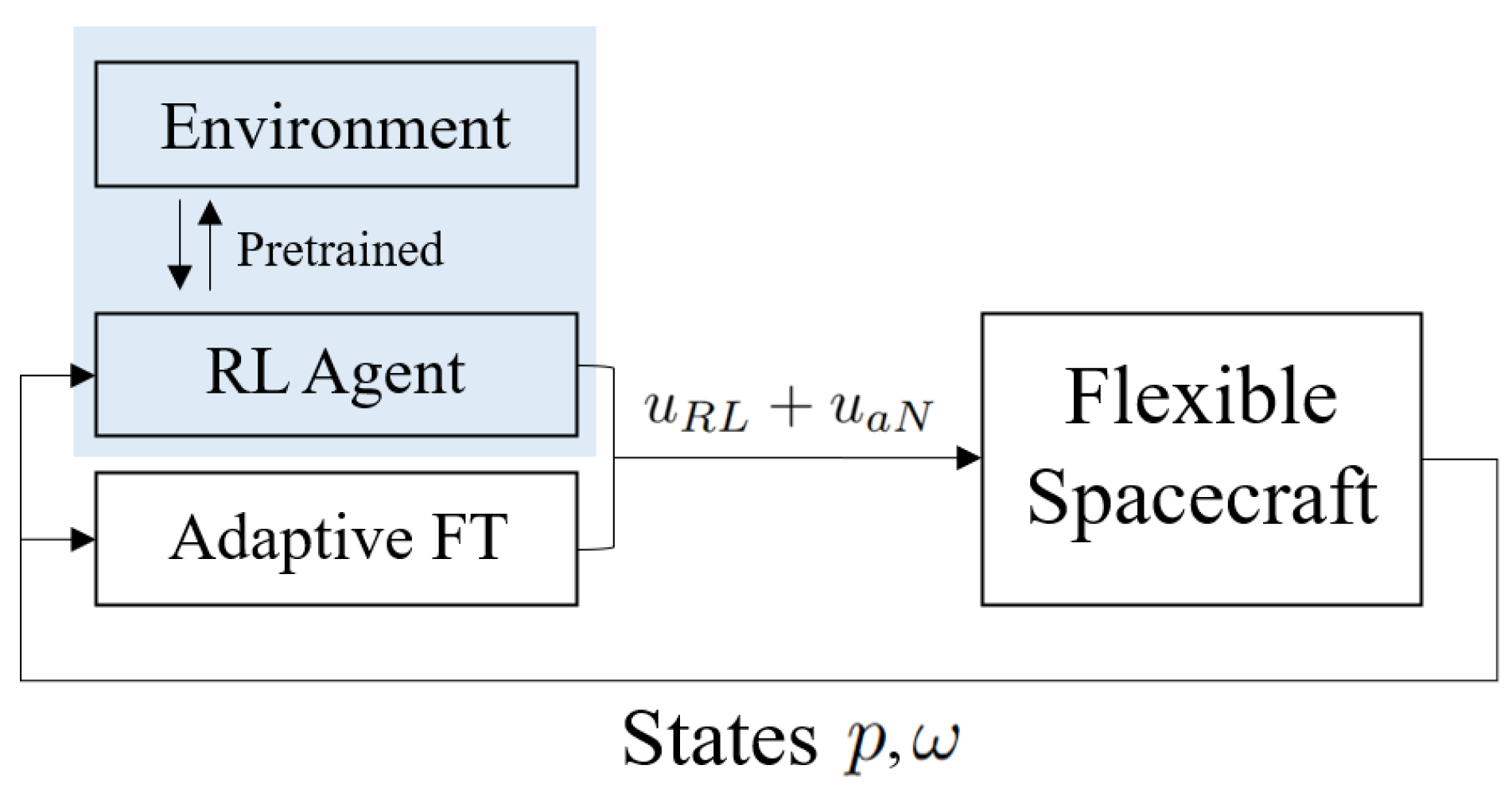
The controller is structured as

$$\mathit{u}={\mathit{u}}_{RL}+{\mathit{u}}_{aN},$$

(16)

where ${\mathit{u}}_{RL}$ is the nominal controller generated by the trained TD3 agent, and ${\mathit{u}}_{aN}$ is the fault-tolerant controller used for compensating actuator faults. The pretrained TD3 agent is integrated into the composite control framework, as shown in Figure 1.

Based on the standard sliding mode manifold design framework, the sliding manifold is constructed as follows:

$$\mathit{s}=\mathbf{\Gamma }\left\{\mathit{\omega }\left(t\right)-\mathit{\omega }\left(t_0\right)-{\int }_{t_0}^t{\mathit{J}}^{-1}\left[-\mathit{\omega }{\left(\sigma \right)}^{\times }(\mathit{J}\mathit{\omega }+{\mathit{\delta }}^T\dot{\mathit{\eta }})-{\mathit{\delta }}^T\ddot{\mathit{\eta }}+{\mathit{u}}_{\mathrm{RL}}\right]d\sigma \right\},$$

(17)

where $\mathbf{\Gamma }\in {\mathbb{R}}^{3\times 3}$ denotes a constant matrix. The matrix $\mathbf{\Gamma }$ is selected such that the product $\mathbf{\Gamma }{\mathit{J}}^{-1}$ is non-singular (invertible). The unmeasurable flexible modal states $\mathit{\eta }$ is calculated by their observer estimates $\widehat{\mathit{\eta }}$ from Section 2.3. It should be noted that at time instant $t=t_0$, the sliding mode surface satisfies $\mathit{s}(\mathit{\omega }\left(t_0\right),t_0)=0$, thereby eliminating the sliding mode reaching phase entirely.

The fault-tolerant compensator is designed as

$${\mathit{u}}_{aN}=\left\{\begin{array}{cc}-\widehat{\alpha }{\displaystyle \frac{{\left(\mathbf{\Gamma }{\mathit{J}}^{-1}\right)}^T\mathit{s}}{∥{\left(\mathbf{\Gamma }{\mathit{J}}^{-1}\right)}^T\mathit{s}∥}},\hfill & \mathrm{if}\widehat{\alpha }∥{\left(\mathbf{\Gamma }{\mathit{J}}^{-1}\right)}^T\mathit{s}∥\ge ϵ\hfill \\ -{\widehat{\alpha }}^2{\displaystyle \frac{{\left(\mathbf{\Gamma }{\mathit{J}}^{-1}\right)}^T\mathit{s}}{ϵ}},\hfill & \mathrm{if}\widehat{\alpha }∥{\left(\mathbf{\Gamma }{\mathit{J}}^{-1}\right)}^T\mathit{s}∥<ϵ\hfill \end{array}\right.$$

(18)

where $ϵ$ is a small positive scalar alleviating undesirable chattering, and $\widehat{\alpha }\ge 0$ is obtained by the following adaptive law:

$$\dot{\widehat{\alpha }}=\gamma \left(∥{\left(\mathbf{\Gamma }{\mathit{J}}^{-1}\right)}^T\mathit{s}∥-\lambda \widehat{\alpha }\right),\mathrm{with}\widehat{\alpha }\left(0\right)\ge 0$$

(19)

where $\gamma$ and $\lambda$ denote positive scalar constants, and the second term $-\lambda \widehat{\alpha }$ serves to enhance robustness against external disturbances and unmodeled dynamic characteristics, while mitigating the excessive growth of the adaptive gain parameter. In this work, these parameters are set to $\gamma =10.0$ and $\lambda =2.5\times {10}^{-4}$, with the initial adaptive gain $\widehat{\alpha }\left(0\right)=1.0$ and the boundary layer thickness $ϵ=0.01$.

The fault-tolerant mechanism of the compensator (18) can be understood through the integral-type sliding mode (ISM) principle. By construction of the sliding manifold (17), the nominal rigid–flexible dynamics are embedded in the integral term; differentiating $\mathit{s}$ cancels these nominal terms and yields (23), where only the fault, disturbance, and the deviation $\mathit{u}-{\mathit{u}}_{\mathrm{RL}}$ remain. When the compensator maintains $\mathit{s}=0$, the condition $\dot{\mathit{s}}=0$ enforces $({\mathit{I}}_3-\mathit{E})\mathit{u}+\overline{\mathit{u}}+\mathit{d}={\mathit{u}}_{\mathrm{RL}}$, i.e., the equivalent control exactly counterbalances the fault and disturbance effects. Substituting this relation back into (3) recovers the nominal fault-free dynamics driven solely by ${\mathit{u}}_{\mathrm{RL}}$. Hence, the actuator effectiveness loss $\mathit{E}\left(t\right)$, additive fault $\overline{\mathit{u}}$, and disturbance $\mathit{d}$ are all algebraically rejected on the sliding manifold—without requiring explicit fault identification. The compensator (18) enforces this sliding motion: its direction ${(\mathbf{\Gamma }{\mathit{J}}^{-1})}^T\mathit{s}/\parallel {(\mathbf{\Gamma }{\mathit{J}}^{-1})}^T\mathit{s}\parallel$ is the steepest-descent direction for the Lyapunov function ${\displaystyle \frac{1}{2}}{\mathit{s}}^T\mathit{s}$, and the adaptive gain $\widehat{\alpha }$ in (19) self-tunes to dominate the unknown combined fault–disturbance magnitude, thereby guaranteeing reachability without prior knowledge of the fault bounds.

4.2. Stability Analysis

Lemma 1.

Based on the switching gain update rule in (19), $\widehat{\alpha }$ is upper bounded. In other words, for all $t>0$, there exists a positive scalar $\overline{\alpha }$ satisfying

$$\widehat{\alpha }\le \overline{\alpha },\alpha \le \overline{\alpha },\forall t>0,$$

where α is expressed as $\alpha ={\displaystyle \frac{\sqrt{3}{e}_m{u}_{\max }+{\overline{u}}_m+d_m+\epsilon }{1-e_m}},$ with $u_{\max }$ denoting the upper bound of the RL output, $e_m$, $d_m$, and ${\overline{u}}_m$ defined in Assumptions 1–3, and ϵ being a bounded positive constant.

Proof. 

The proof follows the same lines as in the appendix of [28]. Therefore, it is omitted here. The essential idea is as follows. Consider the Lyapunov candidate $V_s={\displaystyle \frac{1}{2}}{\mathit{s}}^T\mathit{s}$, whose derivative along the closed-loop trajectories satisfies ${\dot{V}}_s\le -(1-e_m)(\widehat{\alpha }-\alpha )\parallel {(\mathbf{\Gamma }{\mathit{J}}^{-1})}^{T}s\parallel$, where $\alpha$ is the finite constant defined above. To establish boundedness of $\widehat{\alpha }$, four mutually exclusive cases are examined based on whether $\widehat{\alpha }$ exceeds $\alpha$ and whether $\parallel {(\mathbf{\Gamma }{\mathit{J}}^{-1})}^{T}s\parallel$ exceeds a small threshold related to the $\sigma$-modification parameter $\lambda$. In each case, either ${\dot{V}}_s\le 0$ or the comparison principle is invoked, and in all cases a uniform upper bound for $\widehat{\alpha }$ is established. □

Theorem 1.

Consider the flexible spacecraft attitude kinematics and dynamics described by (1) and (3) in the presence of fault described by (4). Suppose that Assumptions 1–3 hold and only the boundedness of actuator faults/disturbances is known (their upper bounds are unknown). Under the action of the adaptive controller in (16) and the adaptive law in (19), the system trajectories are able to enter a bounded region around the sliding manifold $\mathit{s}=0$ in finite time.

Proof. 

First, construct the candidate Lyapunov function that fuses the sliding manifold error and the adaptive gain estimation error:

$$V={\displaystyle \frac{1}{2}}{\mathit{s}}^T\mathit{s}+{\displaystyle \frac{1-e_m}{2\gamma }}{\left(\widehat{\alpha }-\overline{\alpha }\right)}^2,$$

(20)

where $\overline{\alpha }$ is the upper bound of $\widehat{\alpha }$ defined in Lemma 1, and $\gamma >0$ is the adaptive gain. We analyze the time derivative $\dot{V}$ in two cases based on the boundary layer of the smoothed control ${\mathit{u}}_{aN}$, as defined in Equation (18).

Case I: $\widehat{\alpha }∥{(\mathbf{\Gamma }{\mathit{J}}^{-1})}^T\mathit{s}∥\ge ϵ$

Taking the time derivative of Equation (17), the first-order derivative of the sliding surface is obtained as

$$\dot{\mathit{s}}=\mathbf{\Gamma }\left\{\dot{\mathit{\omega }}\left(t\right)-{\mathit{J}}^{-1}\left[-\mathit{\omega }{\left(t\right)}^{\times }(\mathit{J}\mathit{\omega }\left(t\right)+{\mathit{\delta }}^T\dot{\mathit{\eta }}\left(t\right))-{\mathit{\delta }}^T\ddot{\mathit{\eta }}\left(t\right)+{\mathit{u}}_{\mathrm{RL}}\left(t\right)\right]\right\}.$$

(21)

Multiplying both sides of Equation (3) by ${\mathit{J}}^{-1}$ and rearranging terms, the angular velocity derivative $\dot{\mathit{\omega }}$ is solved as

$$\dot{\mathit{\omega }}={\mathit{J}}^{-1}\left[-{\mathit{\omega }}^{\times }\left(\mathit{J}\mathit{\omega }+{\mathit{\delta }}^T\dot{\mathit{\eta }}\right)-{\mathit{\delta }}^T\ddot{\mathit{\eta }}+\left({\mathit{I}}_3-\mathit{E}\left(t\right)\right)\mathit{u}+\overline{\mathit{u}}+\mathit{d}\right].$$

(22)

Substituting Equation (22) into Equation (21) yields

$$\dot{\mathit{s}}=\mathbf{\Gamma }{\mathit{J}}^{-1}\left[\left({\mathit{I}}_3-\mathit{E}\left(t\right)\right)\mathit{u}+\overline{\mathit{u}}+\mathit{d}-{\mathit{u}}_{\mathrm{RL}}\right].$$

(23)

Taking the time derivative of V, and substituting Equation (23), we obtain

$$\begin{array}{cc}\hfill \dot{V}& ={\mathit{s}}^T\dot{\mathit{s}}+{\displaystyle \frac{1-e_m}{\gamma }}\left(\widehat{\alpha }-\overline{\alpha }\right)\dot{\widehat{\alpha }}\hfill \\ \hfill & \le -\left(1-e_m\right)\left[\overline{\alpha }-{\displaystyle \frac{\sqrt{3}{e}_m{u}_{\max }+{\overline{u}}_m+d_m}{1-e_m}}\right]∥{(\mathbf{\Gamma }{\mathit{J}}^{-1})}^T\mathit{s}∥\hfill \\ \hfill & -\lambda (1-e_m)\left(\widehat{\alpha }-\overline{\alpha }\right)\widehat{\alpha }.\hfill \end{array}$$

(24)

From Lemma 1, we have the following key inequalities:

$$\overline{\alpha }-{\displaystyle \frac{\sqrt{3}{e}_m{u}_{\max }+{\overline{u}}_m+d_m}{1-e_m}}\ge {\displaystyle \frac{\epsilon }{1-e_m}},|\widehat{\alpha }-\overline{\alpha }|\le \overline{\alpha }.$$

Substituting these into Equation (24), we further simplify $\dot{V}$ to

$$\begin{array}{cc}\hfill \dot{V}& \le -\lambda (1-e_m)|\widehat{\alpha }-\overline{\alpha }|-\epsilon ∥{(\mathbf{\Gamma }{\mathit{J}}^{-1})}^T\mathit{s}∥+\lambda (1-e_m)\left(|\widehat{\alpha }-\overline{\alpha }|+{\displaystyle \frac{1}{4}}{\overline{\alpha }}^2\right)\hfill \\ \hfill & =-{\delta }_1|\widehat{\alpha }-\overline{\alpha }|-{\delta }_2∥\mathit{s}∥+{\eta }_1,\hfill \end{array}$$

(25)

where ${\delta }_1=\lambda (1-e_m)$, ${\delta }_2=\epsilon ∥\mathbf{\Gamma }{\mathit{J}}^{-1}∥$, and ${\eta }_1=\lambda (1-e_m)\left(\overline{\alpha }+{\displaystyle \frac{1}{4}}{\overline{\alpha }}^2\right)$ are positive scalars. Rewriting Equation (25) in terms of $\sqrt{V}$ (the square root of the Lyapunov function) for finite-time stability analysis:

$$\begin{array}{cc}\hfill \dot{V}& \le -\sqrt{{\displaystyle \frac{2\gamma {\delta }_1^2}{1-e_m}}}\sqrt{{\displaystyle \frac{1-e_m}{2\gamma }}{(\widehat{\alpha }-\overline{\alpha })}^2}-\sqrt{2}{\delta }_2\sqrt{{\displaystyle \frac{1}{2}}{\mathit{s}}^T\mathit{s}}+{\eta }_1\hfill \\ & \le -{\delta }_m{V}^{1/2}+{\eta }_1,\hfill \end{array}$$

where ${\delta }_m=\sqrt{2}\min \left\{\sqrt{{\displaystyle \frac{\gamma {\delta }_1^2}{1-e_m}}},{\delta }_2\right\}$ is a positive constant.

Case II: $\widehat{\alpha }∥{(\mathbf{\Gamma }{\mathit{J}}^{-1})}^T\mathit{s}∥<ϵ$

For the case inside the boundary layer, the time derivative of V (Equation (20)) is derived as

$$\begin{array}{cc}\hfill \dot{V}& =-{\displaystyle \frac{1-e_m}{ϵ}}{\widehat{\alpha }}^2{∥{(\mathbf{\Gamma }{\mathit{J}}^{-1})}^T\mathit{s}∥}^2+(1-e_m)\widehat{\alpha }∥{(\mathbf{\Gamma }{\mathit{J}}^{-1})}^T\mathit{s}∥\hfill \\ \hfill & -(1-e_m)\left[\widehat{\alpha }-{\displaystyle \frac{\sqrt{3}{e}_m{u}_{\max }+{\overline{u}}_m+d_m}{1-e_m}}\right]∥{(\mathbf{\Gamma }{\mathit{J}}^{-1})}^T\mathit{s}∥\hfill \\ \hfill & +(1-e_m)\left(\widehat{\alpha }-\overline{\alpha }\right)∥{(\mathbf{\Gamma }{\mathit{J}}^{-1})}^T\mathit{s}∥-\lambda (1-e_m)\left({\widehat{\alpha }}^2-\widehat{\alpha }\overline{\alpha }\right).\hfill \end{array}$$

(26)

The quadratic term $-{\displaystyle \frac{1-e_m}{ϵ}}{\widehat{\alpha }}^2{∥{(\mathbf{\Gamma }{\mathit{J}}^{-1})}^T\mathit{s}∥}^2+(1-e_m)\widehat{\alpha }∥{(\mathbf{\Gamma }{\mathit{J}}^{-1})}^T\mathit{s}∥$ attains its maximum value ${\displaystyle \frac{(1-e_m)ϵ}{4}}$ at $\widehat{\alpha }∥{(\mathbf{\Gamma }{\mathit{J}}^{-1})}^T\mathit{s}∥={\displaystyle \frac{ϵ}{2}}$. Following the same derivation as Case I and using Lemma 1, we obtain

$$\dot{V}\le -{\delta }_m{V}^{1/2}+{\eta }_2,$$

(27)

where ${\eta }_2={\displaystyle \frac{1-e_m}{4}}\left(\lambda {\overline{\alpha }}^2+4\lambda \overline{\alpha }+ϵ\right)$ is a positive scalar.

Combining Case I and Case II, we obtain a unified inequality for $\dot{V}$ that holds for all $t>0$:

$$\dot{V}\le -{\delta }_m{V}^{1/2}+{\eta }_m,$$

(28)

where ${\eta }_m=\max \{{\eta }_1,{\eta }_2\}={\displaystyle \frac{1-e_m}{4}}\left(\lambda {\overline{\alpha }}^2+4\lambda \overline{\alpha }+ϵ\right)$. From the practical finite-time stability theory for nonlinear systems, the decrease of V drives the system trajectories into the set $V^{1/2}\le {\displaystyle \frac{{\eta }_m}{(1-{\theta }_0){\delta }_m}}$ in finite time, where $0<{\theta }_0<1$ is a positive scalar. For the sliding manifold s, this implies the ultimate boundedness (the system converges to a small neighborhood of $\mathit{s}=0$):

$$\begin{array}{cc}\hfill ∥\mathit{s}∥& \le {\displaystyle \frac{\sqrt{2}{\eta }_m}{(1-{\theta }_0){\delta }_m}}\hfill \\ \hfill & ={\displaystyle \frac{(1-e_m)\left(\lambda {\overline{\alpha }}^2+4\lambda \overline{\alpha }+ϵ\right)}{4(1-{\theta }_0)·\min \left\{\lambda \sqrt{\gamma (1-e_m)},\epsilon ∥\mathbf{\Gamma }{\mathit{J}}^{-1}∥\right\}}}.\hfill \end{array}$$

(29)

Hence, the trajectory of the system remains bounded within a small neighborhood surrounding the sliding manifold $\mathit{s}=0$ over a finite time horizon. This concludes the proof. □

5. Simulation and Discussion

In this section, the training environment settings are introduced and hyperparameter configurations are summarized in

Table 2. Hyperparameter settings.

Parameter	Value
Learning Rates
Actor learning rate (${\alpha }_{\mathrm{actor}}$)	$3\times {10}^{-4}$
Critic learning rate (${\alpha }_{\mathrm{critic}}$)	$3\times {10}^{-4}$
Network Architecture
Hidden layer dimensions	400, 300
Number of hidden layers	2
RL Algorithm Parameters
Discount factor (${\gamma }_{RL}$)	0.99
Soft update coefficient ($\mathit{\tau }$)	0.01
Experience replay buffer size	1,000,000
Minimum buffer size for training	1000
Batch size	250
Policy update delay (d)	3
Exploration noise std (${\sigma }_{\mathrm{explore}}$)	0.1
Target policy noise std ($\sigma$)	0.2
Target noise clip bound (c)	0.5
Optimizer and Reproducibility
Optimizer	Adam
Random seeds (Python, NumPy, PyTorch)	2
Training Schedule
Total training episodes ($N_{\mathrm{episodes}}$)	20,000
Episode length ($T_{\mathrm{episode}}$)	200 steps
Time step duration ($\Delta t$)	1 s

. To systematically assess robustness, five evaluation scenarios (S0–S4) form a progressive uncertainty evaluation framework, as summarized in

Table 3. Configurations of the five evaluation scenarios.

Setting	S0	S1	S2	S3	S4
Measurement noise	—	√	√	√	√
Non-zero initial ${\omega }_0$	—	—	√	—	—
Parameter mismatch	—	—	—	√	√
External disturbance	—	—	—	√	√
Actuator faults	—	—	—	—	√

. Starting from a noise-free baseline (S0), each subsequent scenario introduces an additional source of non-ideality: measurement noise (S1), non-zero initial angular velocity (S2), parameter mismatch and external disturbance (S3), and finally concurrent actuator faults (S4). Detailed scenario configurations are provided in the notes accompanying Table 3.

This section validates the proposed control framework through numerical simulations, organized into three parts. First, the training setup, spacecraft physical parameters, and hyperparameter configurations are documented. Second, the trained TD3 agents are evaluated under fault-free conditions (Scenarios S0–S3), comparing the $\widehat{\mathit{\eta }}$-augmented agent A against the baseline agent $A_0$ to assess the effectiveness of vibration-aware reward shaping. Third, the composite TD3+AFT controller is tested under concurrent actuator faults (Scenario S4) and benchmarked against PD, PD+AFT, and the standalone TD3 agent.

5.1. Training Settings

During the training, each component of the initial attitude ${\mathit{p}}_0$ is independently sampled from the uniform distribution over the interval $[-1,1]$. No measurement noise, parameter perturbation or fault condition is introduced in the training phase. The environment is treated as ideal except for a sinusoidal disturbance ${\mathit{d}}_{\mathrm{train}}\left(t\right)$, as follows:

$$\begin{array}{cc}\hfill d_{\mathrm{train},i}\left(t\right)& =A_i\sin \left({\displaystyle \frac{2\pi }{40}}t+{\varphi }_i\right)+{10}^{-7},i=1,2,3\hfill \\ \hfill A_i& \sim \mathcal{U}(0,0.05)\left[\mathrm{N}·\mathrm{m}\right],i=1,2,3\hfill \\ \hfill {\varphi }_i& \sim \mathcal{U}(0,2\pi )\left[\mathrm{rad}\right],i=1,2,3\hfill \end{array}$$

(30)

The frequency ${\displaystyle \frac{2\pi }{40}}$ rad/s is chosen to be representative and to maintain the same order of magnitude as Equation (34). The amplitude $A_i$ is intentionally set substantially larger than the actual disturbance magnitude. The exaggerated disturbance magnitude and fully randomized phases are designed to expose the agent to a diverse set of disturbance realizations during training, thereby encouraging the learning of robust control policies that generalize beyond the specific disturbance patterns encountered in evaluation.

The inertia matrix $\mathit{J}$ is configured as

$$\mathit{J}=\left[\begin{array}{ccc}120& 3& 4\\ 3& 100& 10\\ 4& 10& 120\end{array}\right]{\mathrm{kg}·\mathrm{m}}^2.$$

(31)

Different from [32], where the off-diagonal components are neglected, this paper takes the inertial coupling into account to better match the practical engineering situation. The flexible parameters are selected with reference to [31]. The number of flexible modes m is set as 4, and the coupling matrix $\mathit{\delta }$ is set as

$$\mathit{\delta }=\left[\begin{array}{ccc}6.45637& 1.27814& 2.15629\\ -1.25819& 0.91756& -1.67264\\ 1.11687& 2.48901& -0.83674\\ 1.23637& -2.65810& -1.12530\end{array}\right].$$

(32)

The flexible modal parameters are given by

$${\omega }_n=\left[\begin{array}{cccc}0.7681& 1.1038& 1.8733& 2.5496\end{array}\right],\xi =\left[\begin{array}{cccc}0.0056& 0.0086& 0.0128& 0.0252\end{array}\right],$$

(33)

where ${\omega }_n$ denotes natural frequencies (rad/s) and $\xi$ represents corresponding damping ratios.

The training procedure follows the standard TD3 protocol [13]. At each timestep, the agent observes the state ${\mathit{s}}_{RL,t}={[{\mathit{p}}^T,{\mathit{\omega }}^T]}^T$, selects an action ${\mathit{a}}_t={\pi }_{\varphi }\left({\mathit{s}}_{RL,t}\right)+{ϵ}_t$ with exploration noise ${ϵ}_t\sim \mathcal{N}(0,{\sigma }_{\mathrm{explore}}^{2}I)$, and receives a reward computed by the phased reward function (13). Transitions are stored in an experience replay buffer of capacity ${10}^6$ and sampled uniformly in minibatches for network updates. Training begins after a warm-up phase of 1000 steps to populate the buffer. The complete hyperparameter configuration is listed in Table 2.

It is worth noting that the later TD3 policy network itself only receives the 6-dimensional state vector ${[{\mathit{p}}^T,{\mathit{\omega }}^T]}^T$ as defined in Section 3.2; the observer-estimated flexible states are used internally by the environment for reward computation and by the AFT control layer, and are never passed to the RL policy network.

The training is implemented in Python 3.10 using PyTorch 1.12.0. The flexible spacecraft environment is simulated with a fixed-step integration using SciPy’s solve_ivp function with the RK45 method at a time step of $\Delta t=1$ s. All simulations are performed on a workstation with an Intel Core i7-13700 CPU and an NVIDIA RTX 3060 GPU; typical training duration is approximately 12 h for 20,000 episodes.

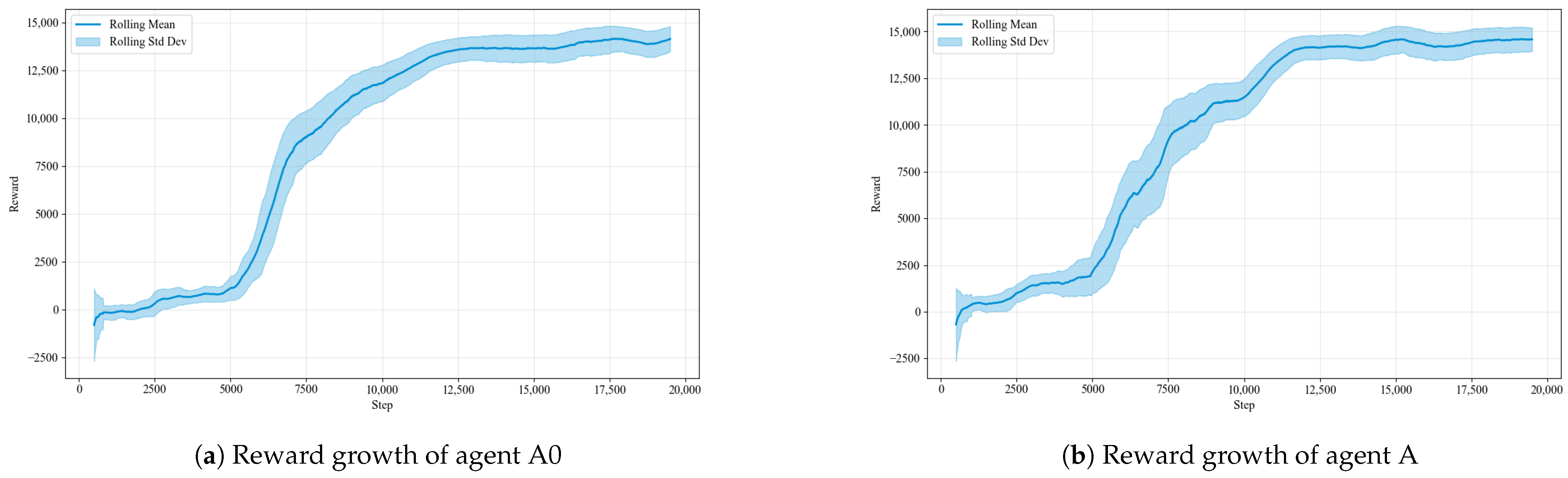
The effectiveness of incorporating the observer-estimated flexible state $\widehat{\mathit{\eta }}$ into the reward function is verified through an ablation experiment that compares the control performance of two agents trained by different reward functions (12) and (13). For clear distinction, the agent trained using the reward function (12) is designated as agent $A_0$, and the agent trained with the reward function (13) is denoted as agent A. The reward accumulation of the two agents is visualized in Figure 2. Both agents exhibit a rapid ascent after approximately 5000 episodes, indicating that the exploration phase transitions into policy exploitation around this point. Agent $A_0$ produces an overall smoother reward curve, whereas agent A exhibits slightly larger fluctuations but converges to a higher steady-state reward value. These differences stem from distinct reward structures: Agent $A_0$ optimizes solely with respect to attitude and angular velocity errors, yielding a simpler and more stationary reward signal; agent A additionally incorporates the observer-estimated flexible modal displacement $\widehat{\mathit{\eta }}$, which enriches the learning signal with vibration-suppression information but simultaneously introduces greater stochasticity due to the coupling between the flexible dynamics and the rigid-body motion. The richer feedback enables agent A to attain a higher asymptotic reward at the cost of moderately increased training variance.

5.2. Test Scenario Settings

To systematically evaluate agent robustness under progressively challenging conditions, five evaluation scenarios (S0–S4) are constructed as a progressive uncertainty evaluation framework. The complete scenario configurations are summarized in Table 3, and each scenario is described in detail below.

All five scenarios share a common initial attitude ${\mathit{p}}_0=[0.3,0.1,-0.2]$, with a simulation duration of 200 s and a time step of 1 s. The target attitude is zero ($\mathit{p}=0$, $\mathit{\omega }=0$) in all cases.

Scenario S0 (pure baseline) represents the simplest evaluation condition: no measurement noise, no parameter mismatch, no external disturbance, and no actuator faults. The spacecraft starts from rest (${\mathit{\omega }}_0=0$) and the controller operates with perfect state information and a perfectly known plant model. This scenario establishes the nominal performance reference against which all subsequent, more challenging scenarios are compared.

Scenario S1 (measurement noise) introduces Gaussian white noise on both the MRP attitude and angular velocity measurements. The noise standard deviations are set to ${\sigma }_p=8.0\times {10}^{-5}$ [33] and ${\sigma }_{\omega }=5\times {10}^{-5}$ rad/s [34]. All other conditions remain identical to S0. This scenario evaluates the agents’ tolerance to realistic sensor imperfections.

Scenario S2 (non-zero initial angular velocity) retains the measurement noise of S1 and additionally assigns a non-zero initial angular velocity ${\mathit{\omega }}_0=[0.02,-0.03,0.04]$ rad/s. The spacecraft thus possesses initial kinetic energy at the start of the maneuver, making the attitude reorientation more demanding than the rest-to-rest cases of S0 and S1.

Scenario S3 (parameter mismatch and external disturbance) layers model-plant mismatch and persistent external disturbance on top of the measurement noise of S1. The parameter mismatch perturbs three off-diagonal elements of the moment of inertia matrix (from nominal values $J_{12}=J_{21}=3$, $J_{13}=J_{31}=4$ to $J_{12}=J_{21}=6$, $J_{13}=J_{31}=7$ kg m²), while the flexible coupling matrix $\mathit{\delta }$, natural frequencies ${\omega }_n$, and damping ratios $\xi$ are all increased by $+10\%$ relative to their nominal values. The external disturbance is a multi-sinusoidal torque adopted from [35]:

$$\mathit{d}\left(t\right)=0.2\times {10}^{-3}·\left[\begin{array}{c}3\cos \left(10{\omega }_{d}t\right)+4\sin \left(3{\omega }_{d}t\right)-10\\ -1.5\sin \left(2{\omega }_{d}t\right)+3\cos \left(5{\omega }_{d}t\right)+15\\ 3\sin \left(10{\omega }_{d}t\right)-8\sin \left(4{\omega }_{d}t\right)+10\end{array}\right]\mathrm{Nm}.$$

(34)

where ${\omega }_d=0.1$ rad/s in this work. The initial angular velocity is zero. Scenario S3 represents the most demanding fault-free condition in the evaluation suite.

Scenario S4 (actuator faults) incorporates all the non-idealities of S3—measurement noise, parameter mismatch, and external disturbance—and adds a time-varying actuator fault profile. Each actuator experiences a partial loss-of-effectiveness fault at $t=10$ s. Subsequently, at $t=50$ s, these actuators are also subjected to an additive time-varying fault, which is injected into the spacecraft dynamics in an additive manner. The parameters in (4) are selected as follows:

$$\begin{array}{cc}\hfill e_i\left(t\right)& =\left\{\begin{array}{cc}0,\hfill & t<10\hfill \\ 0.5,\hfill & t\ge 10\hfill \end{array}\right.\hfill \\ \hfill \overline{\mathit{u}}\left(t\right)& =\left\{\begin{array}{cc}0,\hfill & t<50\hfill \\ 0.3+0.05\sin \left(t\right),\hfill & t\ge 50\hfill \end{array}\right.\hfill \end{array}$$

(35)

The efficiency loss $e_i=0.5$ and the additive bias $\overline{\mathit{u}}=0.3$ together represent a severe fault condition relative to the maximum actuator torque $u_{\max }=1$ N·m: the actuators lose half of their control effectiveness while being simultaneously subjected to a constant offset of $0.3$ N·m, corresponding to static actuator anomalies such as sudden installation misalignment, mechanical wear, circuit zero-point drift, or long-term aging-induced output bias. The sinusoidal term $0.05\sin \left(t\right)$, introduces a time-varying component into the additive fault term, capturing the fact that actuator faults may not remain constant but can evolve over time—for instance, due to mechanical/electrical periodic perturbations such as reaction wheel bearing periodic friction, thruster jet pulsation, or electromagnetic circuit ripple.

This scenario represents the most challenging condition in the evaluation suite, testing the agents’ resilience to concurrent sensor noise, modeling errors, environmental disturbances, and actuator degradation.

Scenarios S0–S3 are designed to compare the performance of agent A and agent $A_0$, demonstrating the benefit of incorporating the observer-estimated flexible modal state $\widehat{\mathit{\eta }}$ into the reward function. Scenario S4 serves as the validation platform for the adaptive fault-tolerant (AFT) control framework, where four control schemes are evaluated and compared under concurrent actuator faults.

5.3. Fault-Free Scenarios

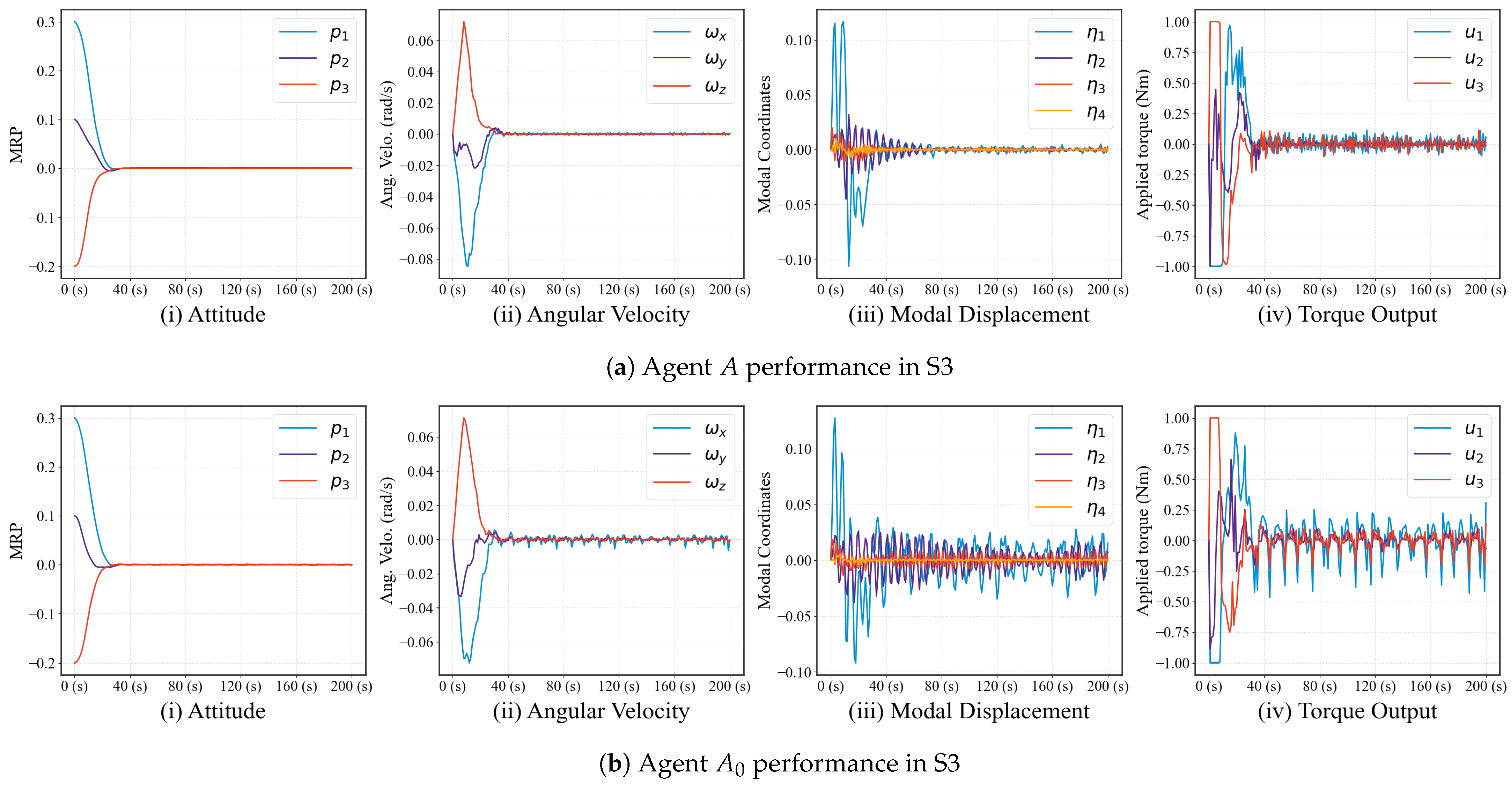
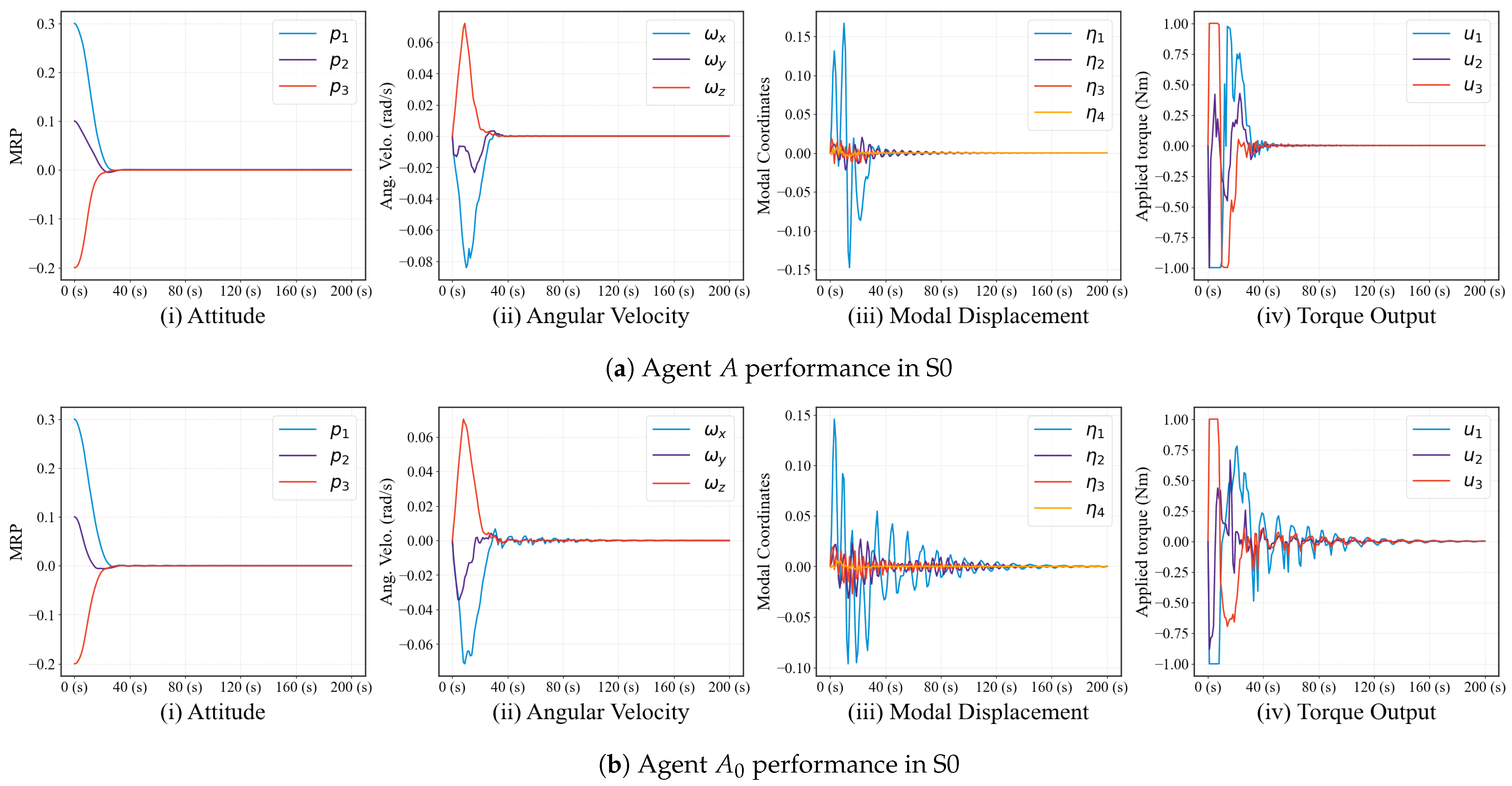
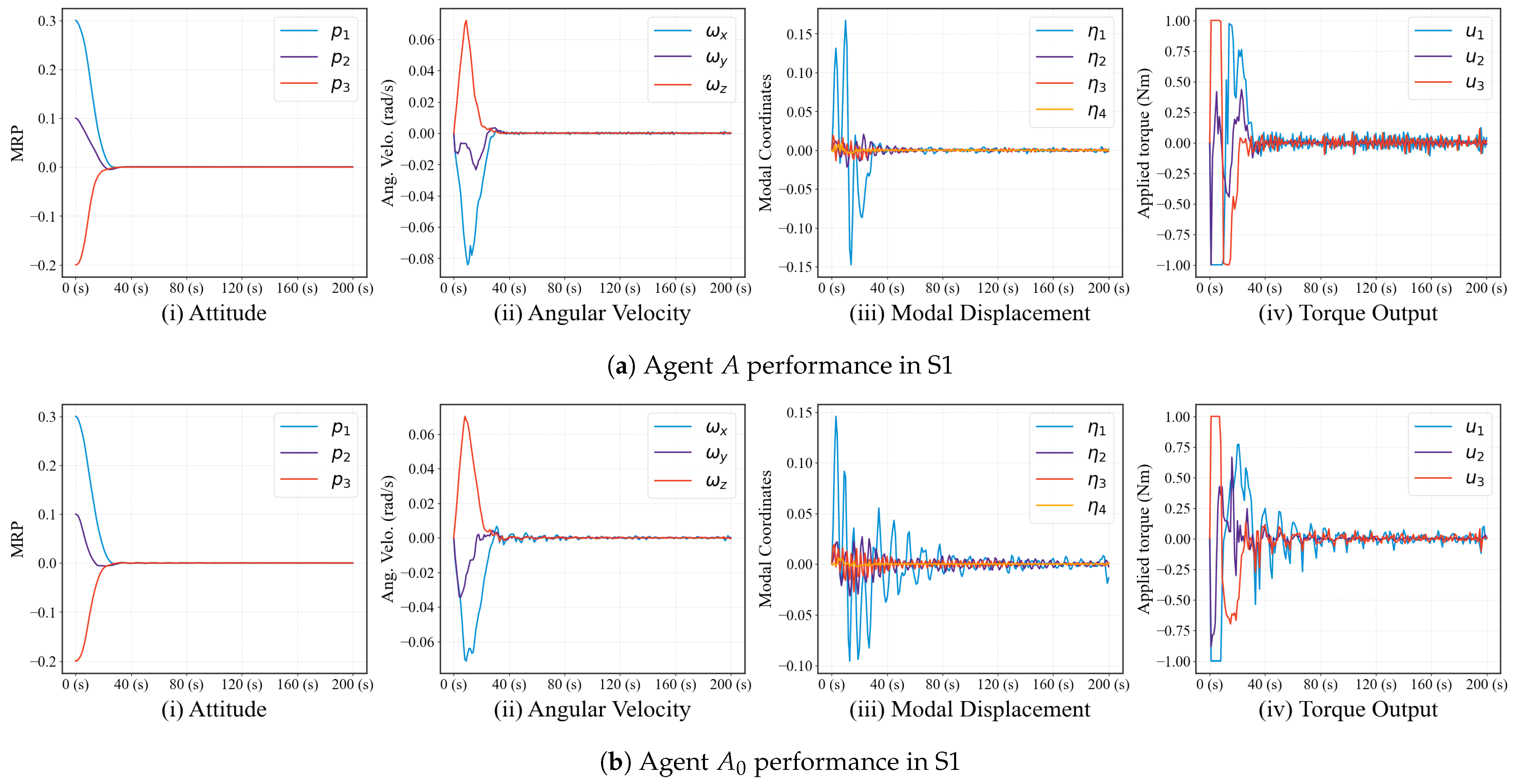
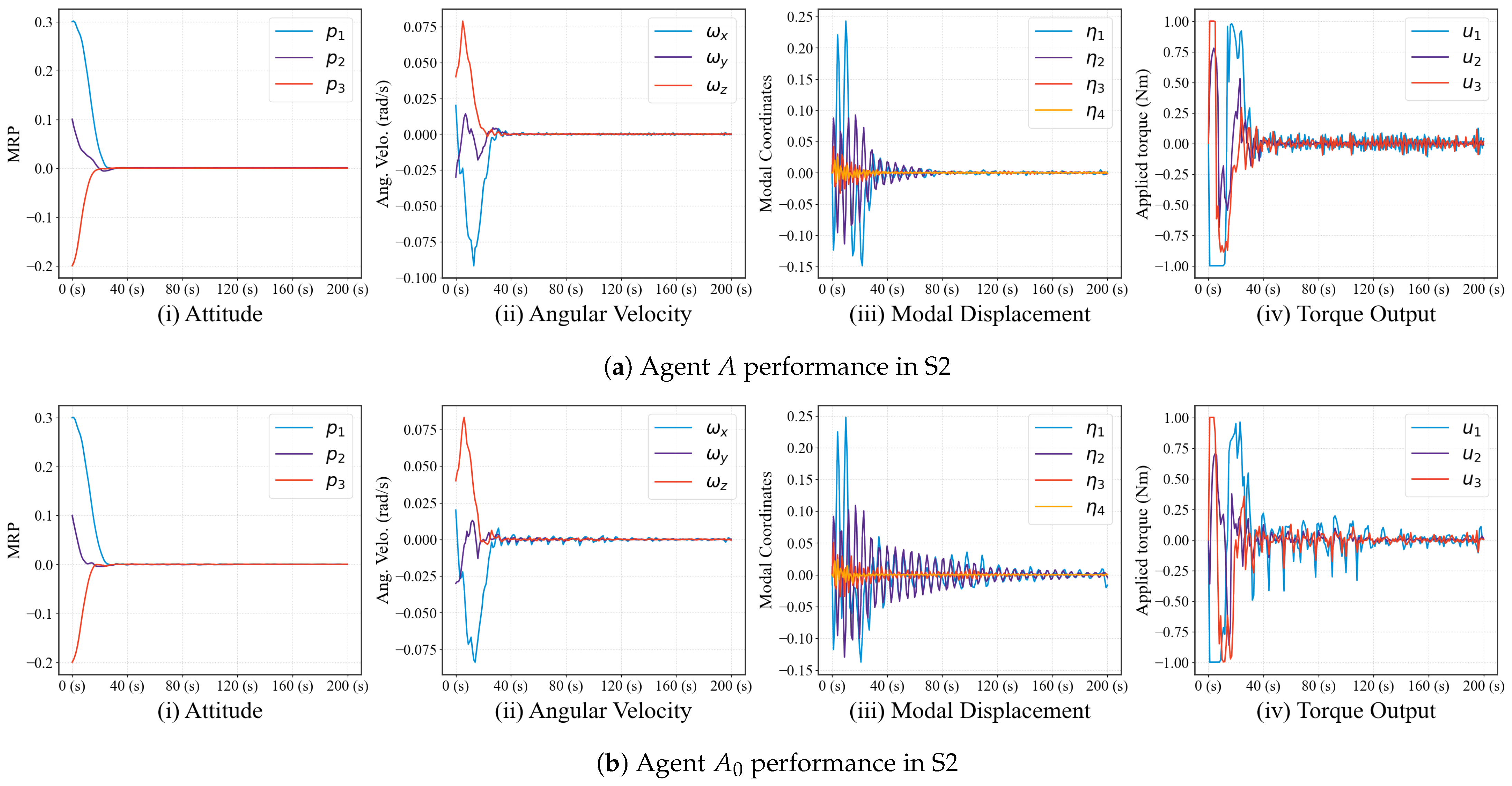
The performance of agent A and agent $A_0$ under S0–S3 is visualized in Figure 3, Figure 4, Figure 5 and Figure 6. Each figure presents the time histories of the MRP attitude, angular velocity, control torque output, and flexible modal displacement for both agents in a side-by-side comparison.

Across all four scenarios, agent A consistently exhibits noticeably cleaner trajectories with reduced oscillations and smaller vibration peaks, whereas agent $A_0$ often produces persistent back-and-forth chattering in the control output accompanied by sustained flexible-mode excitation. This difference is a direct consequence of the $\widehat{\mathit{\eta }}$-augmented reward function (13): by rewarding the suppression of the observer-estimated modal displacement during training, agent A learns a policy that inherently avoids control actions that would excite the flexible modes. The resulting closed-loop behavior achieves simultaneous attitude regulation and vibration damping, yielding smoother state trajectories and a cleaner control effort. In contrast, agent $A_0$, trained without any vibration-related feedback (12), optimizes only for attitude errors and may inadvertently induce and sustain flexible oscillations, which manifest as noisier signals and persistent torque chattering.

To provide a quantitative assessment, steady-state performance metrics (computed over $t>160$ s) of both agents across S0–S3 are summarized in

Table 4. Quantitative comparison of agent A vs A0 across Scenarios S0–S3 (steady-state, $t>160$ s).

Scenario	Agent	${\parallel \mathit{p}\parallel }_{\mathit{\infty }}$	${\parallel \mathit{\omega }\parallel }_{\mathit{\infty }}$ (rad/s)	$\mathit{\eta }$ RMS	${\mathit{\eta }}_{0.01}$ (s)	u RMS (Nm)
S0	A	$4.57\times {10}^{-4}$	$7.00\times {10}^{-6}$	$5.00\times {10}^{-5}$	30	$6.16\times {10}^{-4}$
	A0	$2.87\times {10}^{-4}$	$1.17\times {10}^{-4}$	$6.87\times {10}^{-4}$	95	$4.91\times {10}^{-3}$
S1	A	$5.44\times {10}^{-4}$	$9.97\times {10}^{-4}$	$2.24\times {10}^{-3}$	30	$5.80\times {10}^{-2}$
	A0	$3.63\times {10}^{-4}$	$1.72\times {10}^{-3}$	$5.50\times {10}^{-3}$	—	$4.89\times {10}^{-2}$
S2	A	$5.44\times {10}^{-4}$	$9.95\times {10}^{-4}$	$2.25\times {10}^{-3}$	56	$5.79\times {10}^{-2}$
	A0	$4.02\times {10}^{-4}$	$1.83\times {10}^{-3}$	$6.85\times {10}^{-3}$	—	$4.95\times {10}^{-2}$
S3	A	$6.55\times {10}^{-4}$	$1.12\times {10}^{-3}$	$2.32\times {10}^{-3}$	42	$6.33\times {10}^{-2}$
	A0	$8.91\times {10}^{-4}$	$6.54\times {10}^{-3}$	$1.94\times {10}^{-2}$	—	0.194

. The metrics include the steady-state infinity norms of the MRP attitude (${\parallel \mathit{p}\parallel }_{\infty }$) and angular velocity (${\parallel \mathit{\omega }\parallel }_{\infty }$), the root mean square (RMS) of the flexible modal displacement vector norm ($\eta$ RMS) as a measure of residual vibration energy, the settling time of the flexible modal displacement (${\eta }_{0.01}$), and the RMS of the applied control torque (u RMS) as a measure of control effort. Here ${\eta }_{0.01}$ is defined as the earliest time after which the peak absolute modal displacement across all four flexible modes ($\max \left(\right|{\eta }_1|,|{\eta }_2|,|{\eta }_3|,|{\eta }_4\left|\right)$) remains permanently below $0.01$, i.e., the vibration settling time. “—” denotes failure to converge within the 200 s evaluation horizon.

The quantitative results in Table 4 reveal several important findings. First, in terms of vibration suppression, agent A consistently and substantially outperforms agent $A_0$ across all four scenarios. Compared with agent $A_0$, agent A reduces the $\eta$ RMS by approximately $92.7\%$ (S0), $59.3\%$ (S1), $67.2\%$ (S2), and $88.0\%$ (S3). Correspondingly, compared with agent $A_0$, agent A reduces ${\eta }_{0.01}$ (vibration settling time) by $68.4\%$ (S0); in all other scenarios, agent $A_0$ fails to converge within the 200 s evaluation horizon. This demonstrates that the $\widehat{\mathit{\eta }}$-augmented reward function (13) provides a robust and generalizable vibration suppression capability that persists even as non-idealities accumulate.

Second, a consistent trade-off between attitude pointing accuracy and vibration suppression is observed. Although agent A achieves better vibration damping across all scenarios, agent $A_0$ attains marginally better pointing accuracy in S0–S2, at the cost of severely degraded vibration damping. However, in S3, the most demanding fault-free scenario, agent A surpasses agent $A_0$ across all metrics including attitude pointing (${\parallel \mathit{p}\parallel }_{\infty }=6.55\times {10}^{-4}$ vs. $8.91\times {10}^{-4}$), indicating that the $\widehat{\mathsf{\eta }}$-guided policy learns a more robust control strategy that does not sacrifice pointing accuracy under compound uncertainties.

Third, the torque expenditure of agent A is moderately higher than that of agent $A_0$ across S1–S2 (e.g., $5.80\times {10}^{-2}$ vs. $4.89\times {10}^{-2}$ Nm in S1), reflecting the additional control effort required for active vibration suppression. In S3, however, agent A achieves substantially lower torque RMS ($6.33\times {10}^{-2}$ vs. $0.194$ Nm), demonstrating that under compound uncertainties the $\widehat{\mathit{\eta }}$-guided policy simultaneously delivers superior vibration attenuation and higher control efficiency. In S0, agent A achieves significantly lower torque RMS ($6.16\times {10}^{-4}$ vs. $4.91\times {10}^{-3}$ Nm), indicating that in the absence of perturbations, the learned policy achieves both superior vibration attenuation and higher control efficiency.

Overall, the ablation study across S0–S3 confirms that incorporating the observer-estimated flexible modal displacement $\widehat{\mathit{\eta }}$ into the reward function enables the agent to strike a better balance between attitude pointing accuracy and vibration suppression. The resulting policy generalizes effectively across diverse non-ideal conditions at a modest increase in control effort under perturbed scenarios.

5.4. Fault Scenario

Given that agent A demonstrated superior vibration suppression and robust performance across S0–S3 in the ablation study, its trained policy weights are adopted as the TD3 nominal controller in this section. Four control architectures are compared under Scenario S4: (i) pure PD (${\mathit{u}}_{pd}=-k_p\mathit{p}-k_d\mathit{\omega }$ with $k_p=30$, $k_d=60$), (ii) pure TD3, (iii) PD augmented with the AFT compensator (PD+AFT), and (iv) TD3 augmented with the AFT compensator (TD3+AFT).

To evaluate the adaptability of the proposed control framework under actuator fault conditions, Scenario S4 is employed, whose configuration is detailed in Section 5.2. This simulation validates the efficacy of the composite control framework proposed in Section 4.

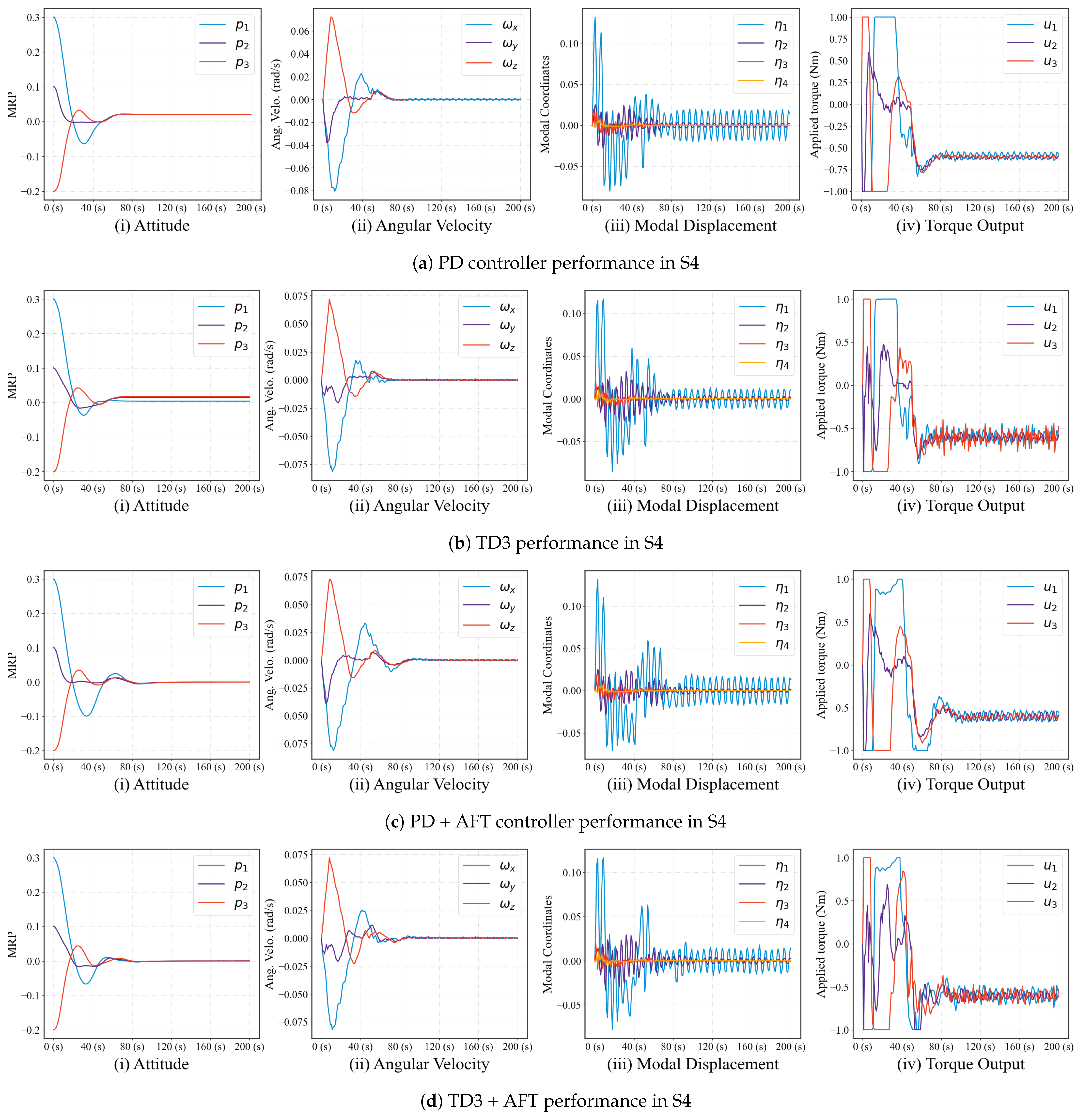
The simulation outcomes of the four control architectures under S4 are illustrated in Figure 7. To further provide a quantitative assessment, key performance metrics are summarized in

Table 5. Quantitative comparison of four control methods under Scenario 4 (actuator faults).

	PD	TD3	PD+AFT	TD3+AFT
Steady-state ($t>160$ s)
MRP ${\parallel \mathit{p}\parallel }_{\infty }$	$2.02\times {10}^{-2}$	$1.75\times {10}^{-2}$	$5.81\times {10}^{-4}$	$4.04\times {10}^{-4}$
${\parallel \mathit{\omega }\parallel }_{\infty }$ (rad/s)	$8.43\times {10}^{-4}$	$8.54\times {10}^{-4}$	$8.34\times {10}^{-4}$	$7.54\times {10}^{-4}$
$\eta$ RMS	$1.37\times {10}^{-2}$	$8.43\times {10}^{-3}$	$1.17\times {10}^{-2}$	$1.04\times {10}^{-2}$
Torque RMS (Nm)	$1.042$	1.045	1.044	1.044
Transient/full-trajectory
Peak ${\parallel \mathit{\eta }\parallel }_{\infty }$	0.132	$0.117$	0.132	$0.117$
Peak ${\parallel \mathit{\omega }\parallel }_{\infty }$ (rad/s)	$8.05\times {10}^{-2}$	$8.12\times {10}^{-2}$	$8.12\times {10}^{-2}$	$8.22\times {10}^{-2}$
Integrated $\eta$ RMS	$2.98\times {10}^{-2}$	$2.91\times {10}^{-2}$	$3.03\times {10}^{-2}$	$2.91\times {10}^{-2}$
MRPs converge to $0.005$ (s)	—	—	94	74
Integrated Torque RMS (Nm)	$1.082$	1.086	$1.112$	1.118

.

In Table 5, all steady-state metrics are computed over $t>160$ s. Integrated Torque RMS is computed over the full trajectory. Peak ${\parallel \mathit{\eta }\parallel }_{\infty }$ and peak ${\parallel \mathit{\omega }\parallel }_{\infty }$ capture the maximum values over the entire 200 s trajectory. Integrated $\eta$ RMS is computed over the full trajectory as a proxy for total vibration energy. MRPs converging to $0.005$ indicates the earliest time after which ${\parallel \mathit{p}\parallel }_{\infty }$ remains below $0.005$ (“—” denotes failure to converge within 200 s).

Several observations can be drawn from the quantitative comparison in Table 5. First, AFT augmentation is essential for precise convergence under actuator faults: pure PD and pure TD3 both fail to bring the MRP error below $0.005$ within the 200 s evaluation horizon, whereas TD3+AFT achieves this threshold at 74 s and PD+AFT at 94 s. The proposed TD3+AFT architecture delivers the best overall pointing accuracy, reducing ${\parallel \mathit{p}\parallel }_{\infty }$ by a factor of approximately 43.3 relative to pure TD3 ($1.75\times {10}^{-2}$ vs. $4.04\times {10}^{-4}$) and by a factor of approximately 50.0 relative to pure PD ($2.02\times {10}^{-2}$ vs. $4.04\times {10}^{-4}$).

Second, TD3 consistently outperforms PD across all transient and steady-state vibration metrics. In steady state, TD3 achieves $\eta$ RMS of $8.43\times {10}^{-3}$ compared to $1.37\times {10}^{-2}$ for PD, representing a 38.5% reduction. Among AFT-augmented architectures, TD3+AFT achieves lower $\eta$ RMS ($1.04\times {10}^{-2}$ vs. $1.17\times {10}^{-2}$ for PD+AFT). In the transient phase, TD3 and TD3+AFT tie for the lowest peak ${\parallel \mathit{\eta }\parallel }_{\infty }$ (both $0.117$) and integrated $\eta$ RMS (both $2.91\times {10}^{-2}$), confirming that the learned TD3 policy inherently produces smoother maneuvers with reduced flexible mode excitation.

Third, a comparison between the two AFT-augmented methods shows that TD3+AFT achieves better pointing accuracy, convergence speed, and vibration suppression: 30.5% lower steady-state ${\parallel \mathit{p}\parallel }_{\infty }$ ($4.04\times {10}^{-4}$ vs. $5.81\times {10}^{-4}$), 21.3% faster MRP convergence (74 s vs. 94 s), and 11.1% lower steady-state $\eta$ RMS ($1.04\times {10}^{-2}$ vs. $1.17\times {10}^{-2}$). PD+AFT retains marginal advantages in peak angular velocity (${\parallel \mathit{\omega }\parallel }_{\infty }$: $8.12\times {10}^{-2}$ vs. $8.22\times {10}^{-2}$ rad/s) and integrated torque RMS ($1.112$ vs. $1.118$ N·m), though the differences are small. Overall, the learned TD3 nominal policy coordinates with the AFT compensator more effectively than the fixed-gain PD law, as the RL agent learns to generate control actions that complement the fault-tolerant layer rather than compete with it.

Regarding control effort, all four controllers operate within the $u_{\max }=1$ N·m actuator saturation limit stated in Section 3.2. The steady-state torque RMS values are tightly clustered ($1.042$–$1.045$ N·m), and the integrated torque RMS also remains within a narrow band ($1.082$–$1.118$ N·m). The fact that TD3+AFT achieves substantially superior pointing and vibration performance while expending comparable control effort indicates that both the RL policy and the AFT layer contribute to control efficiency in complementary ways: the TD3 agent provides smooth nominal commands that minimize unnecessary actuation, while the AFT compensator injects targeted corrections only when faults are active.

6. Conclusions

This study focuses on the attitude maneuver problem of flexible spacecraft under external disturbances, flexible dynamics, and actuator faults. An integrated control framework combining TD3-based RL agent with an adaptive fault-tolerant compensator is proposed. Simulation results demonstrate that incorporating the observer-estimated flexible modal displacement into the reward function enables the RL agent to learn active vibration suppression while maintaining competitive attitude accuracy. Under actuator faults, the AFT compensator significantly improves control precision, and the composite TD3+AFT architecture achieves the best pointing accuracy, convergence speed, and vibration suppression among all configurations, while maintaining comparable control effort. The RL agent and AFT compensator operate in a complementary manner: the RL agent provides smooth nominal commands that inherently suppress flexible mode excitation, while the AFT layer injects targeted fault-tolerant corrections when needed.

Future work includes experimental validation on physical testbeds to assess performance under real sensing and actuation imperfections beyond the Gaussian noise models used in the present simulations. Additionally, extending the RL policy to support on-orbit incremental learning would enable real-time adaptation to evolving spacecraft parameters and fault conditions, further improving the controller’s generalization capability in complex operational environments.

References

1. Golestani, M.; Zhang, W.; Yang, Y.; Xuan-Mung, N. Disturbance observer-based constrained attitude control for flexible spacecraft. IEEE Trans. Aerosp. Electron. Syst. 2022, 59, 963–972. [Google Scholar] [CrossRef]
2. He, G.; Cao, D. Dynamic Modeling and Attitude–Vibration Cooperative Control for a Large-Scale Flexible Spacecraft. Actuators 2023, 12, 167. [Google Scholar] [CrossRef]
3. Shahid, F.; Luo, H.; Jiang, Y.; Noman Hasan, M. Finite-Time Adaptive Sliding Mode Fault-Tolerant Attitude Control for Flexible Spacecraft. IEEE Trans. Control Syst. Technol. 2025, 33, 1700–1711. [Google Scholar] [CrossRef]
4. Dian, W.; Yunhua, W.; Hongyi, X.; Franco, B.Z.; Chen, X. Scheduled input shaping based attitude agile control for flexible spacecraft with vibration suppression. Aerosp. Sci. Technol. 2025, 164, 110355. [Google Scholar] [CrossRef]
5. Zhong, C.; Chen, Z.; Guo, Y. Attitude Control for Flexible Spacecraft with Disturbance Rejection. IEEE Trans. Aerosp. Electron. Syst. 2017, 53, 101–110. [Google Scholar] [CrossRef]
6. Song, G.; Agrawal, B.N. Vibration suppression of flexible spacecraft during attitude control. Acta Astronaut. 2001, 49, 73–83. [Google Scholar] [CrossRef]
7. Yu, Y.; Meng, X.; Li, K.; Xiong, F. Robust control of flexible spacecraft during large-angle attitude maneuver. J. Guid. Control. Dyn. 2014, 37, 1027–1033. [Google Scholar] [CrossRef]
8. Angeletti, F.; Iannelli, P.; Gasbarri, P.; Sabatini, M. End-to-end design of a robust attitude control and vibration suppression system for large space smart structures. Acta Astronaut. 2021, 187, 416–428. [Google Scholar]
9. Khoroshylov, S.; Martyniuk, S.; Sushko, O.; Vasyliev, V.; Medzmariashvili, E.; Woods, W. Dynamics and attitude control of space-based synthetic aperture radar. Nonlinear Eng. 2023, 12, 20220277. [Google Scholar] [CrossRef]
10. Izzo, D.; Märtens, M.; Pan, B. A survey on artificial intelligence trends in spacecraft guidance dynamics and control. Astrodynamics 2019, 3, 287–299. [Google Scholar] [CrossRef]
11. Khoroshylov, S.V.; Redka, M.O. Deep learning for space guidance, navigation, and control. Space Sci. Technol. 2021, 27, 38–52. [Google Scholar]
12. Silvestrini, S.; Lavagna, M. Deep learning and artificial neural networks for spacecraft dynamics, navigation and control. Drones 2022, 6, 270. [Google Scholar] [CrossRef]
13. Fujimoto, S.; Hoof, H.; Meger, D. Addressing function approximation error in actor-critic methods. In Proceedings of the International Conference on Machine Learning, PMLR, Stockholm, Sweden, 10–15 July 2018; pp. 1587–1596. [Google Scholar]
14. Hong, D.; Lee, S.; Cho, Y.H.; Baek, D.; Kim, J.; Chang, N. Energy-Efficient Online Path Planning of Multiple Drones Using Reinforcement Learning. IEEE Trans. Veh. Technol. 2021, 70, 9725–9740. [Google Scholar] [CrossRef]
15. Abo Mosali, N.; Shamsudin, S.S.; Alfandi, O.; Omar, R.; Al-Fadhali, N. Twin Delayed Deep Deterministic Policy Gradient-Based Target Tracking for Unmanned Aerial Vehicle with Achievement Rewarding and Multistage Training. IEEE Access 2022, 10, 23545–23559. [Google Scholar] [CrossRef]
16. Zhang, D.; Li, X.; Ren, G.; Yao, J.; Chen, K.; Li, X. Three-Dimensional Path Planning of UAVs in a Complex Dynamic Environment Based on Environment Exploration Twin Delayed Deep Deterministic Policy Gradient. Symmetry 2023, 15, 1371. [Google Scholar] [CrossRef]
17. Yan, T.; Liu, C.; Gao, M.; Jiang, Z.; Li, T. A Deep Reinforcement Learning-Based Intelligent Maneuvering Strategy for the High-Speed UAV Pursuit-Evasion Game. Drones 2024, 8, 309. [Google Scholar] [CrossRef]
18. Zhou, T.; Liu, Z.; Jin, W.; Han, Z. Intelligent maneuver decision-making for UAVs using the TD3–LSTM reinforcement learning algorithm under uncertain information. Front. Robot. AI 2025, 12, 1645927. [Google Scholar] [CrossRef] [PubMed]
19. Zhang, Z.; Li, X.; An, J.; Man, W.; Zhang, G. Model-Free Attitude Control of Spacecraft Based on PID-Guide TD3 Algorithm. Int. J. Aerosp. Eng. 2020, 2020, 8874619. [Google Scholar] [CrossRef]
20. Gao, M.; Yan, T.; Li, Q.; Fu, W.; Zhang, J. Intelligent Pursuit–Evasion Game Based on Deep Reinforcement Learning for Hypersonic Vehicles. Aerospace 2023, 10, 86. [Google Scholar] [CrossRef]
21. Zhu, J.; Tang, W.; Dong, J. Design of Intelligent Controller for Aero-engine Based on TD3 Algorithm. Inf. Technol. Control 2023, 52, 1010–1024. [Google Scholar] [CrossRef]
22. Cheng, Y.; Chen, L.; Chen, C.L.P.; Wang, X. Off-Policy Deep Reinforcement Learning Based on Steffensen Value Iteration. IEEE Trans. Cogn. Dev. Syst. 2021, 13, 1023–1032. [Google Scholar] [CrossRef]
23. Shi, J.; Liu, X.; Cai, G.; Liu, F.; Sun, J.; Zhu, D. Reinforcement Learning for Cooperative Control of the Ultra-Close Flexible Spacecraft Formation Flying. IEEE Aerosp. Electron. Syst. Mag. 2026, 41, 54–68. [Google Scholar] [CrossRef]
24. Li, Y.; Zhang, F.; Gao, Z. Attitude control for dumbbell-shaped spacecraft subject to parameter uncertainty via fully-actuated system approach and deep reinforcement learning. Int. J. Syst. Sci. 2026, 1–18. [Google Scholar] [CrossRef]
25. El-Dalahmeh, G.; Jabbarpour, M.R.; Vo, B.Q.; Kowalczyk, R. Intelligent Spacecraft Attitude Fault Recovery Using Deep Reinforcement Learning. IEEE Access 2026, 14, 6238–6260. [Google Scholar]
26. Henna, H.; Toubakh, H.; Kafi, M.R.; Gürsoy, Ö.; Sayed-Mouchaweh, M.; Djemai, M. Satellite fault tolerant attitude control based on expert guided exploration of reinforcement learning agent. J. Exp. Theor. Artif. Intell. 2025, 37, 987–1011. [Google Scholar]
27. Mahfouz, A.; Valiullin, A.; Lukashevichus, A.; Pritykin, D. Reinforcement learning for attitude control of A spacecraft with flexible appendages. In Proceedings of the 73rd International Astronautical Congress. International Astronautical Federation, Paris, France, 18–22 September 2022. [Google Scholar]
28. Shen, Q.; Wang, D.; Zhu, S.; Poh, E.K. Integral-Type Sliding Mode Fault-Tolerant Control for Attitude Stabilization of Spacecraft. IEEE Trans. Control Syst. Technol. 2015, 23, 1131–1138. [Google Scholar] [CrossRef]
29. Terzakis, G.; Lourakis, M.; Ait-Boudaoud, D. Modified Rodrigues Parameters: An Efficient Representation of Orientation in 3D Vision and Graphics. J. Math. Imaging Vis. 2018, 60, 422–442. [Google Scholar] [CrossRef]
30. Zou, A.M.; De Ruiter, A.H.J.; Dev Kumar, K. Distributed attitude synchronization control for a group of flexible spacecraft using only attitude measurements. Inf. Sci. 2016, 343–344, 66–78. [Google Scholar] [CrossRef]
31. Di Gennaro, S. Output stabilization of flexible spacecraft with active vibration suppression. IEEE Trans. Aerosp. Electron. Syst. 2003, 39, 747–759. [Google Scholar] [CrossRef]
32. Peng, Z.; Shen, Q.; Song, C. Attitude Control of Spacecraft Based on Deep Reinforcement Learning TD3 Algorithm. In Proceedings of the International Conference on Guidance, Navigation and Control; Springer: Singapore, 2024; pp. 318–327. [Google Scholar] [CrossRef]
33. Zou, A.M.; Fan, Z. Fixed-time attitude tracking control for rigid spacecraft without angular velocity measurements. IEEE Trans. Ind. Electron. 2019, 67, 6795–6805. [Google Scholar] [CrossRef]
34. Javaid, U.; Basin, M.V.; Ijaz, S. Spacecraft Attitude Stabilization Control Under Actuator Faults and Input Saturation. In Proceedings of the 2024 IEEE 18th International Conference on Advanced Motion Control (AMC), Kyoto, Japan; IEEE: Piscataway, NJ, USA, 2024; pp. 1–6. [Google Scholar] [CrossRef]
35. Hu, Q.; Li, B.; Qi, J. Disturbance observer based finite-time attitude control for rigid spacecraft under input saturation. Aerosp. Sci. Technol. 2014, 39, 13–21. [Google Scholar] [CrossRef]
Figure 1. Composite controller.
Aerospace 13 00571 g001
Figure 2. Reward growth of agents trained by different reward functions.
Aerospace 13 00571 g002
Figure 3. Agent performance comparison in Scenario S0 (pure baseline).
Aerospace 13 00571 g003
Figure 4. Agent performance comparison in Scenario S1 (measurement noise).
Aerospace 13 00571 g004
Figure 5. Agent performance comparison in Scenario S2 (measurement noise + non-zero ω 0 ).
Aerospace 13 00571 g005
Figure 6. Agent performance comparison in Scenario S3 (measurement noise + parameter mismatch + external disturbance).
Aerospace 13 00571 g006
Figure 7. Performance comparison of four control architectures under Scenario S4 (actuator faults).
Aerospace 13 00571 g007