Online Trajectory Optimization Based on Pseudospectra Convex Optimization for Morphing Gliding Reentry Vehicles

Abstract

Trajectory planning for morphing gliding reentry vehicles is a nonconvex optimization problem driven by nonlinearity, parameter uncertainty, and multiple constraints. No-fly zones (NFZs) are a critical constraint because their rapid movement and expansion hinder the real-time generation of optimal flight trajectories and wing morphing strategies. Therefore, this study proposes an innovative online trajectory optimization method based on sequential convex optimization integrated with a deep neural network (DNN). The proposed method first uses the Radau pseudospectral method to discretize continuous dynamics and convert the non-convex trajectory planning problem into a relaxed convex subproblem. The subproblem is reformulated as an augmented Lagrangian function through linearization and is iteratively solved using the interior-point method. Finally, the DNN learns the mapping between flight states and optimal control variables (angle of attack rate, bank angle rate, and wing sweep angle rate) to rapidly generate control variables. Different from the time-consuming offline optimization method, the proposed model only requires 0.4 ms to predict three groups of control variables, with the predicted control errors remaining below 2.25%. This method efficiently provides high-precision and stable reentry trajectories and morphing strategies for gliding reentry vehicles. Thus, the proposed method achieves synchronous flight path and wing deformation optimization and demonstrates strong robustness under time-varying mission conditions.

1. Introduction

Morphing gliding reentry vehicles have several advantages, including high maneuverability, flexible trajectories, and robust anti-interception capabilities [1,2]. These vehicles have been extensively researched by major global aerospace powers because of their wide velocity profiles and extended operational altitudes [3,4]. Among the related technologies, trajectory planning is crucial for analyzing the performance of aircraft, such as range, maneuverability, and ballistic characteristics. This allows morphing gliding reentry vehicles to achieve optimal flight performance by altering wing shapes according to different mission scenarios (e.g., take-off, cruise, reconnaissance, attack, and landing).

Trajectory planning typically requires solving nonlinear optimal control problems under various constraints, including boundary conditions, shape parameter constraints, no-fly-zone (NFZ) constraints, and path constraints [5]. Previous research primarily categorizes proposed trajectory planning algorithms into indirect and direct methods [6,7]. The indirect method derived from Pontryagin’s maximum principle transforms the trajectory optimization problem into a Hamiltonian boundary value problem, which is typically solved using gradient-based algorithms, and offers high solution accuracy and strong optimality. The direct method primarily adopts parameterization to convert the optimal control problem into a parameter optimization problem that is solved using nonlinear programming methods such as the sequential quadratic programming algorithm. This method has been widely investigated because of its intuitive formulation [8,9,10]; however, its unpredictable solution times and unstable convergence restrict its application to online scenarios [11].

Within the direct method, convex optimization frameworks meet the requirements for rapid computational solutions, which increase their utility in spacecraft trajectory optimization [12,13,14,15]. These frameworks excel in solving low-complexity problems and deliver results quickly using interior-point methods. However, most aerospace-related problems are constrained by nonlinear, nonconvex dynamics, and path constraints, which cannot be directly solved within the convex optimization framework. Therefore, a convexification method that effectively minimizes approximation errors is necessary. The mainstream convexification methods include lossless and sequential convexification [16].

To address the Mars landing trajectory planning problem, Ackimese et al. utilized a lossless convexification method. This approach efficiently replaces nonconvex constraints with relaxed convex constraints without compromising the solution accuracy [17,18]. For reentry trajectory optimization, the sequential convex programming (SCP) methodology proposed by Liu et al. differentiates energy-related dynamic equations and integrates linearization and relaxation operations within iterations [13,19,20,21]. The feasibility of this methodology was substantiated by the minimum time and minimum heat flow reentry trajectories. Furthermore, Wang and Zhang improved the conventional SCP algorithm with two enhanced strategies, line-search SCP and trust-region SCP, which significantly enhanced its convergence performance [22]. Zhou et al. proposed an improved SCP method using an adaptive mesh refinement [23], which balanced computational efficiency and solution accuracy by dynamically adjusting the node distribution according to the linearization error after each iteration.

However, the SCP methodology requires further improvements in terms of discretization, convergence, and penalty parameter selection. The classic trapezoidal discretization approach has been used to convert continuous optimization problems into a discrete form [22,24]. Nevertheless, it often introduces considerable discrepancies between the approximation and actual models during computation. To improve the solution accuracy, the density of the equidistant discretization nodes must be increased. This inevitably increases the number of optimization variables and significantly extends the solution time. In contrast, the pseudospectral discretization method achieves higher precision without increasing the number of nodes and has been widely applied to solve optimal control problems [14,25]. Nevertheless, most studies have investigated trajectory optimization for conventional aircraft with fixed configurations, while rarely addressing morphing strategies during flight. For a fixed-configuration aircraft, trajectory optimization aims to obtain the optimal trajectory described by time-varying variables, including the angle of attack, velocity, altitude, and flight-path angle.

Morphing gliding reentry vehicles require the generation of optimal trajectories and the determination of the optimal wing morphing strategy under dynamic mission conditions. The complexity and uncertainty associated with actual flight missions have increased considerably. For instance, no-fly zones in combat regions can be altered at any time. In these scenarios, a vehicle must generate a feasible and safe trajectory, which circumvents restricted zones, ensures flight safety, and satisfies mission constraints by adjusting its wing configuration and other external parameters accordingly. Accordingly, establishing an efficient online trajectory optimization framework that satisfies the practical demands of complex morphing–gliding reentry missions is critical.

However, the application of convex optimization to online trajectory optimization is limited by the real-time requirements and convergence performance. Next-generation artificial intelligence has advanced significantly in numerous fields, and its applications in aerospace guidance, control, and dynamics have been increasingly explored [26,27,28], resulting in several promising achievements. Sanchez-Sanchez and Izzo investigated a deep neural network (DNN) for optimal state-feedback control of nonlinear systems and developed a real-time optimal control architecture [29] capable of handling numerous distinct initial conditions and maintaining optimal feedback responses. Li et al. exploited the strong approximation capabilities and high computational efficiencies of DNNs and used these networks to rapidly generate real-time control commands [30]. Even under deviations from nominal conditions, the framework generates high-precision control commands and exhibits favorable generalization performance. However, research on real-time optimal trajectory generation for morphing gliding reentry vehicles operating in time-varying NFZ environments is insufficient. To address this limitation, this study investigates trajectory optimization and morphing strategies for such vehicles. An online trajectory optimization framework is proposed, which integrates an improved sequential convexification method and a DNN to improve the trajectory planning performance for morphing vehicles.

The remainder of this paper is organized as follows: Section 2 presents an online trajectory optimization scheme that combines deep neural networks and Radau pseudospectral sequential convex optimization. Section 3 presents numerical simulations to verify the effectiveness of the proposed method. Finally, Section 4 concludes the paper.

2. Materials and Methods

2.1. Aerodynamics and Modeling of Morphing Gliding Reentry Vehicle

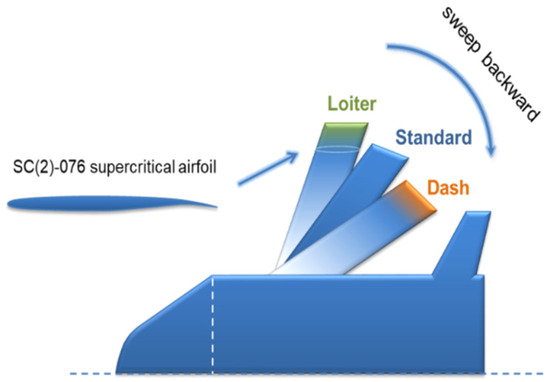
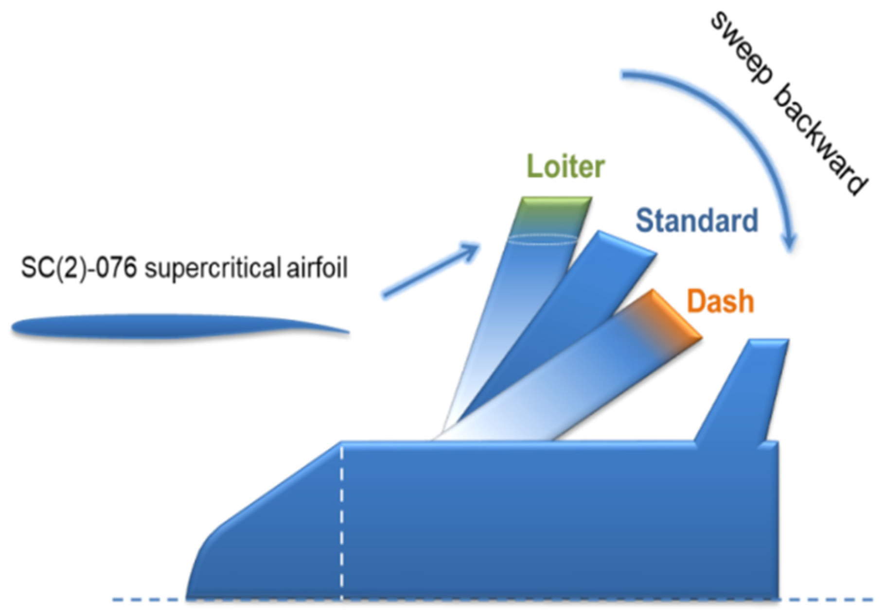
In this study, the morphing–gliding reentry vehicles designed in a prior study [31], which consists of two movable components (left and right wings) and a fixed fuselage, were investigated. The wing sweep angle varies smoothly between 20° and 90°. As illustrated in Figure 1, this morphing vehicle has three typical configurations, namely, the loiter, sweep, and dash configurations with sweep angles of 20°, 40°, and 60°, respectively. The wing parameters for the three configurations are listed in

Table 1. Wing parameters of three configurations.

Configuration	Loiter	Standard	Dash
Sweep, $\mathsf{\Lambda }$ (°)	20	40	60
Sx (m)	−0.093	−0.198	−0.283
Pitch moment of inertia of each wing Ixy (kg m2)	0.6	2.4	4.4
Span (m)	1.99	1.73	1.36

.

A detailed aerodynamic analysis of this morphing gliding reentry vehicle under three configurations, which analyzes flight conditions with Mach numbers of 2, 4, 5, and 7, and angles of attack ranging from −2° to 10°, is presented [32]. In addition, approximate formulas for the aerodynamic behavior are provided. Because the lift and drag coefficients can be approximated as linear and quadratic functions of the angle of attack, respectively, they were modeled as functions of multiple variables, including the angle of attack ($\alpha$), Mach number ($M$), and sweep angle ($\mathsf{\Lambda }$), as follows:

$$\begin{array}{l}{C}_L=C_L^0(M,\overline{\mathsf{\Lambda }})+C_L^{\alpha }(M,\overline{\mathsf{\Lambda }})\alpha +\mathsf{\Delta }{C}_L\\ C_D=C_D^0(M,\overline{\mathsf{\Lambda }})+C_D^{\alpha }(M,\overline{\mathsf{\Lambda }})\alpha +C_D^{{\alpha }^2}(M,\overline{\mathsf{\Lambda }}){\alpha }^2+\mathsf{\Delta }{C}_D\end{array}$$

(1)

where the terms ${\mathsf{\Delta }C}_L$ and $\mathsf{\Delta }{C}_D$ quantify the aerodynamic uncertainty coefficients. The variable $M$ denotes the Mach number, and $\overline{\mathsf{\Lambda }}$ represents the normalized sweep angle, defined by the equation $\overline{\mathsf{\Lambda }}=(\mathsf{\Lambda }-20)/70$, where $\overline{\mathsf{\Lambda }}\in \left[\mathrm{0,1}\right]$. Based on the three typical configurations and four Mach numbers, the coefficients of $C_D^0(M,\overline{\mathsf{\Lambda }})$, $C_D^{\alpha }(M,\overline{\mathsf{\Lambda }})$, $C_D^{{\alpha }^2}(M,\overline{\mathsf{\Lambda }})$, $C_L^0(M,\overline{\mathsf{\Lambda }})$, and $C_L^{\alpha }(M,\overline{\mathsf{\Lambda }})$ are described by the following functions:

$$\begin{array}{l}\begin{array}{l}{C}_D^0=-3.116\times {10}^{-2}-6.272\times {10}^{-3}\overline{\mathsf{\Lambda }}+9.989\times {10}^{-2}M\\ +4.593\times {10}^{-3}{\overline{\mathsf{\Lambda }}}^2-3.722\times {10}^{-3}\overline{\mathsf{\Lambda }}M-4.037\times {10}^{-2}{M}^2\\ -8.766\times {10}^{-4}{\overline{\mathsf{\Lambda }}}^{2}Mn+1.125\times {10}^{-3}\overline{\mathsf{\Lambda }}{M}^2+6.118\times {10}^{-3}{M}^3\\ +8.732\times {10}^{-5}{\overline{\mathsf{\Lambda }}}^2{M}^2-8.575\times {10}^{-5}\overline{\mathsf{\Lambda }}{M}^3-3.143\times {10}^{-4}{M}^4\end{array}\\ \begin{array}{l}{C}_D^{\alpha }=2.037\times {10}^{-3}-4.622\times {10}^{-3}\overline{\mathsf{\Lambda }}+4.129\times {10}^{-4}M\\ +2.728\times {10}^{-3}{\overline{\mathsf{\Lambda }}}^2+2.229\times {10}^{-3}\overline{\mathsf{\Lambda }}M-1.909\times {10}^{-4}{M}^2\\ -1.189\times {10}^{-3}\overline{\mathsf{\Lambda }}M-2.98\times {10}^{-4}\overline{\mathsf{\Lambda }}{M}^2+2.783\times {10}^{-5}{M}^3\\ +1.106\times {10}^{-4}{\overline{\mathsf{\Lambda }}}^2{M}^2+1.083\times {10}^{-5}\overline{\mathsf{\Lambda }}{M}^3-1.322\times {10}^{-6}{M}^4\end{array}\\ \begin{array}{l}{C}_D^{{\alpha }^2}=9.879\times {10}^{-4}+1.743\times {10}^{-4}\overline{\mathsf{\Lambda }}-1.408\times {10}^{-4}M\\ -4.794\times {10}^{-4}{\overline{\mathsf{\Lambda }}}^2-3.67\times {10}^{-5}\overline{\mathsf{\Lambda }}M-3.129\times {10}^{-5}{M}^2\\ +1.292\times {10}^{-4}{\overline{\mathsf{\Lambda }}}^{2}M+3.196\times {10}^{-7}\overline{\mathsf{\Lambda }}{M}^2+9.769\times {10}^{-6}{M}^3\\ -1.057\times {10}^{-5}{\overline{\mathsf{\Lambda }}}^2{M}^2+3.356\times {10}^{-7}\overline{\mathsf{\Lambda }}{M}^3-6.292\times {10}^{-7}{M}^4\end{array}\\ \begin{array}{l}{C}_L^0=0.2186-0.228\overline{\mathsf{\Lambda }}-0.1676M+0.1008{\overline{\mathsf{\Lambda }}}^2\\ +0.127\overline{\mathsf{\Lambda }}M+5.618\times {10}^{-2}{M}^2-4.77\times {10}^{-2}{\overline{\mathsf{\Lambda }}}^{2}M\\ -2.006\times {10}^{-2}\overline{\mathsf{\Lambda }}{M}^2-7.836\times {10}^{-3}{M}^3+4.627\times {10}^{-3}{\overline{\mathsf{\Lambda }}}^2{M}^2\\ +9.454\times {10}^{-4}\overline{\mathsf{\Lambda }}{M}^3+3.866\times {10}^{-4}{M}^4\end{array}\\ \begin{array}{l}{C}_L^{\alpha }=5.183\times {10}^{-2}-1.395\times {10}^{-3}\overline{\mathsf{\Lambda }}-1.626\times {10}^{-3}M\\ -2.217\times {10}^{-2}{\overline{\mathsf{\Lambda }}}^2+4.354\times {10}^{-3}\overline{\mathsf{\Lambda }}M-4.733\times {10}^{-2}{M}^2\\ +4.556\times {10}^{-3}{\overline{\mathsf{\Lambda }}}^{2}M-9.406\times {10}^{-4}\overline{\mathsf{\Lambda }}{M}^2+1.036\times {10}^{-3}{M}^3\\ -3.023\times {10}^{-4}{\overline{\mathsf{\Lambda }}}^2{M}^2+5.77\times {10}^{-5}\overline{\mathsf{\Lambda }}{M}^3-6.171\times {10}^{-5}{M}^4\end{array}\end{array}$$

(2)

2.2. Dynamic Model and Constraints

2.2.1. Dynamic Model in the Distance Domain

To generate the trajectory of a vehicle, its dynamic model is typically non-dimensionalized in the time domain. The nondimensional dynamic equations are formulated as

$$\left\{\begin{array}{l}\dot{r}=V\sin \gamma \\ \dot{\theta }={\displaystyle \frac{V\cos \gamma \sin \psi }{\cos \varphi }}\\ \dot{\varphi }={\displaystyle \frac{V\cos \gamma \cos \psi }{r}}\\ \dot{V}=-D-{\displaystyle \frac{\sin \gamma }{r^2}}+{\omega }_e^{2}r\cos \varphi (\sin \gamma \cos \varphi -\cos \gamma \cos \psi \sin \varphi )\\ \dot{\gamma }={\displaystyle \frac{L\cos \sigma }{V}}-{\displaystyle \frac{\cos \gamma }{r^{2}V}}+{\displaystyle \frac{V\cos \gamma }{r}}+2{\omega }_e\cos \varphi \sin \psi \\ +{\displaystyle \frac{{\omega }_e^{2}r\cos \varphi (\cos \varphi \cos \gamma +\cos \psi \sin \varphi \sin \gamma )}{V}}\\ \dot{\psi }={\displaystyle \frac{L\sin \sigma }{V\cos \gamma }}+{\displaystyle \frac{V\cos \gamma \sin \psi \tan \varphi }{r}}+2{\omega }_e(\sin \varphi -\cos \varphi \tan \gamma \cos \psi )\\ +{\displaystyle \frac{{\omega }_e^{2}r\sin \varphi \cos \varphi \sin \psi )}{V\cos \gamma }}\end{array}\right.$$

(3)

The radial distance between the vehicle and Earth’s center is denoted by r, with the radius of the Earth (R₀) as the nondimensional parameter ($R_0=6378\mathrm{km}$). The spherical coordinates are defined by the longitude $\theta$ and latitude $\varphi$. $V$ is the flight speed of the aircraft, and its nondimensional parameter is $V_c=\sqrt{g_0{R}_0}$. $\gamma$, $\psi$, $\sigma$, and ${\omega }_e$ denote the flight path angle, heading angle, bank angle, and angular rotation rate of the Earth, respectively. The temporal domain is normalized using the time scale $t_c=\sqrt{R_0/g_0}$. $L$ and $D$, which represent the nondimensional lift and drag accelerations, are given by

$$\left\{\begin{array}{l}L=R_0\rho V^2{A}_{ref}{C}_L/2m\\ D=R_0\rho V^2{A}_{ref}{C}_D/2m\end{array}\right.$$

(4)

Here, m, $A_{ref}$, and $\rho$ represent the vehicle mass, aerodynamic reference area, and atmospheric density, respectively, while $C_L$ and $C_D$ represent the lift and drag coefficients, respectively. For the differential kinematic equations with time t as the independent variable, the total flight time must be assigned a fixed value in the reentry trajectory optimization. This limits the flexibility of optimization algorithms when searching for optimal trajectories. To circumvent this limitation, the longitudinal range angle S is adopted as an independent variable of the differential kinematic equations. Thus, the trajectory optimization problem with a fixed terminal time is transformed into one with a fixed terminal range angle. The initial and final boundary values for the longitudinal range angle are defined as follows:

$$s_f=\arccos \left(\sin {\varphi }_0\sin {\varphi }_f+\cos {\varphi }_f\cos {\varphi }_0\cos \left({\theta }_f-{\theta }_0\right)\right)$$

(5)

where ${\theta }_0$ and ${\varphi }_0$ denote the longitudinal and latitudinal coordinates, respectively, of the initial deployment point of the vehicle, while ${\theta }_f$ and ${\varphi }_f$ represent the longitude and latitude of the target destination, respectively.

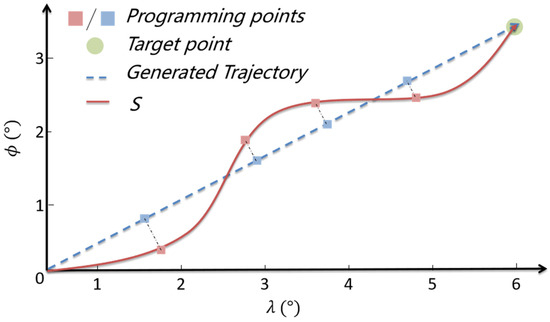
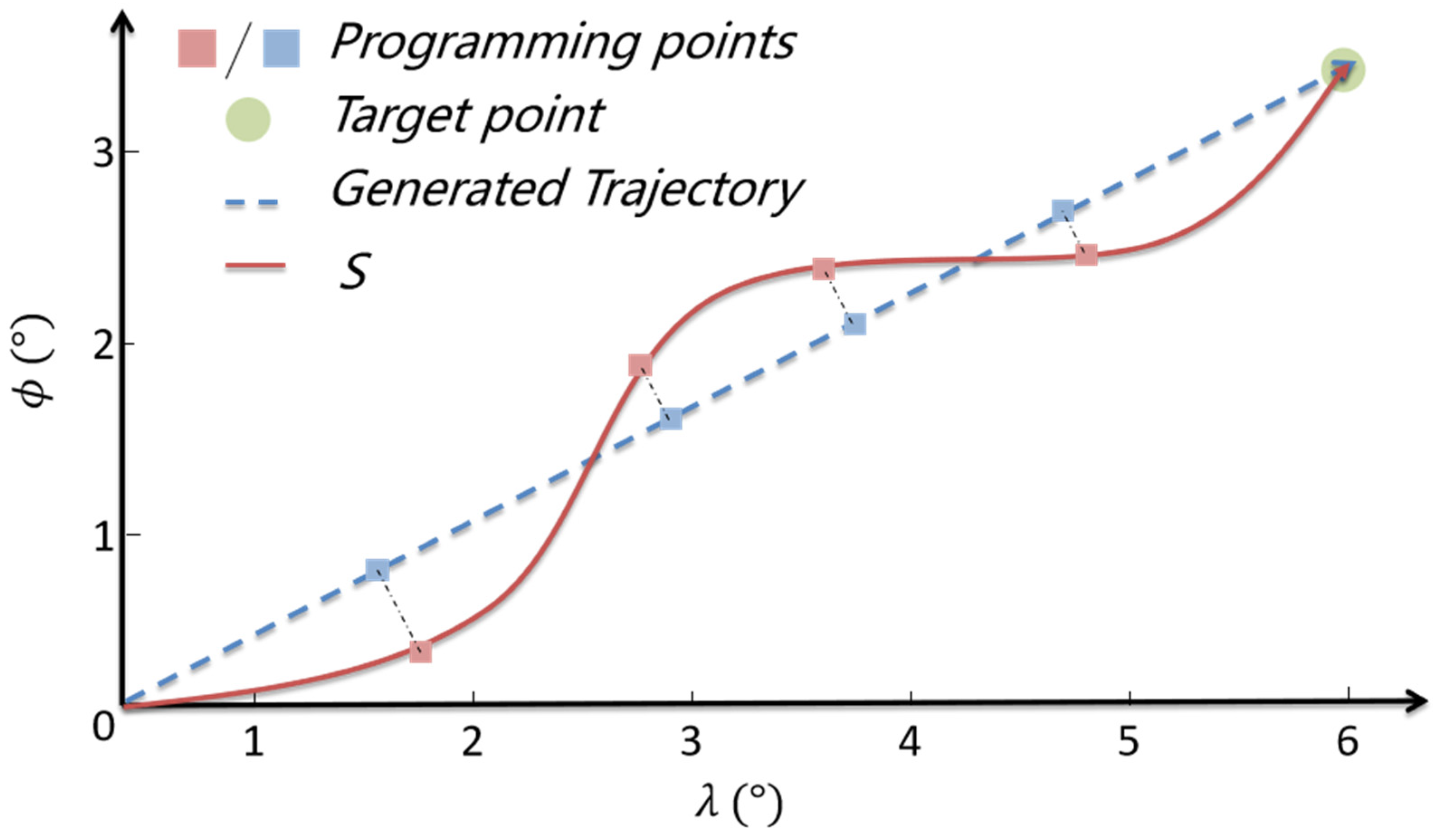
As shown in Figure 2, the problem of generating an effective trajectory can be regarded as the minimization of the projected range between the initial and target points after establishing the initial deployment and target points. $s$ denotes the projected flight path angle. The differential transformation governing the relationship between the time and range domains is formulated as

$$ds/dt=-v\cos \theta /r$$

(6)

By integrating Equations (3) and (6), the dynamic model of the vehicle in the distance domain is expressed as

$$\left\{\begin{array}{l}{\displaystyle \frac{dr}{ds}}=r\tan \gamma \\ {\displaystyle \frac{d\theta }{ds}}={\displaystyle \frac{\sin \psi }{\cos \varphi }}\\ {\displaystyle \frac{d\varphi }{ds}}=\cos \psi \\ {\displaystyle \frac{dV}{ds}}=-{\displaystyle \frac{rD}{V\cos \gamma }}-{\displaystyle \frac{\tan \gamma }{rV}}+{\displaystyle \frac{r^2{\omega }_e^2\cos \varphi (\cos \varphi \tan \gamma -\sin \varphi \cos \psi )}{2}}\\ {\displaystyle \frac{d\gamma }{ds}}={\displaystyle \frac{rL\cos \sigma }{V^2\cos \gamma }}-{\displaystyle \frac{1}{r^{2}V}}+1+{\displaystyle \frac{2r{\omega }_e\cos \varphi \sin \psi }{V\cos \gamma }}\\ +{\displaystyle \frac{r^2{\omega }_e^2\cos \varphi (\cos \varphi \tan \gamma +\cos \psi \sin \varphi \tan \gamma )}{V^2}}\\ {\displaystyle \frac{d\psi }{ds}}={\displaystyle \frac{rL\sin \sigma }{V^2{\cos }^2\gamma }}+\sin \psi \tan \varphi +{\displaystyle \frac{2r{\omega }_e(\sin \varphi -\cos \varphi \tan \gamma \cos \psi )}{V\cos \gamma }}\\ +{\displaystyle \frac{(r^2{\omega }_e^2\sin \varphi \cos \varphi \cos \psi )}{V^2{\cos }^2\gamma }}\end{array}\right.$$

(7)

Here, ${\omega }_e$ denotes the angular rotation rate of the Earth. The flight trajectory is primarily affected by the angle of attack $\alpha$, bank angle $\sigma$, and wing sweep angle $\mathsf{\Lambda }$. To suppress high-frequency oscillations of Λ and avoid excessive loads on control surfaces or structural stress problems caused by rapid state variations, this study designates the time derivatives of these parameters, the rates of change in the angle of attack, bank angle, and the vehicle’s wing leading-edge sweep angle, which are denoted as $\dot{\alpha }$, $\dot{\sigma }$, and $\dot{\mathsf{\Lambda }}$, respectively, as control variables. On this basis, the following augmented differential kinematic equations are obtained:

$$\left\{\begin{array}{l}{\displaystyle \frac{dr}{ds}}=r\tan \gamma \\ {\displaystyle \frac{d\theta }{ds}}={\displaystyle \frac{\sin \psi }{\cos \varphi }}\\ {\displaystyle \frac{d\varphi }{ds}}=\cos \psi \\ {\displaystyle \frac{dV}{ds}}=-{\displaystyle \frac{rD}{V\cos \gamma }}-{\displaystyle \frac{\tan \gamma }{rV}}+{\displaystyle \frac{r^2{\omega }_e^2\cos \varphi (\cos \varphi \tan \gamma -\sin \varphi \cos \psi )}{2}}\\ {\displaystyle \frac{d\gamma }{ds}}={\displaystyle \frac{rL\cos \sigma }{V^2\cos \gamma }}-{\displaystyle \frac{1}{r^{2}V}}+1+{\displaystyle \frac{2r{\omega }_e\cos \varphi \sin \psi }{V\cos \gamma }}\\ +{\displaystyle \frac{r^2{\omega }_e^2\cos \varphi (\cos \varphi \tan \gamma +\cos \psi \sin \varphi \tan \gamma )}{V^2}}\\ {\displaystyle \frac{d\psi }{ds}}={\displaystyle \frac{rL\sin \sigma }{V^2{\cos }^2\gamma }}+\sin \psi \tan \varphi +{\displaystyle \frac{2r{\omega }_e(\sin \varphi -\cos \varphi \tan \gamma \cos \psi )}{V\cos \gamma }}\\ +{\displaystyle \frac{(r^2{\omega }_e^2\sin \varphi \cos \varphi \cos \psi )}{V^2{\cos }^2\gamma }}\\ {\displaystyle \frac{d\alpha }{ds}}=u_{\alpha }\\ {\displaystyle \frac{d\sigma }{ds}}=u_{\sigma }\\ {\displaystyle \frac{d\mathsf{\Lambda }}{ds}}=u_{\mathsf{\Lambda }}\end{array}\right.$$

(8)

2.2.2. Constraint Settings

Throughout the operational reentry phase, the vehicle must adhere to a rigorous set of path constraints, NFZ restrictions, and terminal conditions. The terminal constraints are expressed as

$$\left\{\begin{array}{l}r(s=0)=r_f\hfill \\ v(s=0)=v_f\hfill \\ \varphi (s=0)={\varphi }_f\hfill \\ \theta (s=0)={\theta }_f\hfill \end{array}\hspace{1em}\right.$$

(9)

The parameters $r_f$, $v_f$, ${\varphi }_f$, and ${\theta }_f$ represent the target terminal altitude, terminal velocity, latitude, and longitude, respectively. To ensure flight safety and structural integrity, the trajectory-planning problem is subject to path constraints, including heat flux ${\dot{Q}}_{max}$, dynamic pressure $q_{max}$, and aerodynamic overload $n_{max}$ limits. In addition, the physical feasibility of the actuators is ensured by constraining the rates of change in the angle of attack $\dot{\alpha }$, bank angle $\dot{\sigma }$, and wing leading-edge sweep angle $\dot{\mathsf{\Lambda }}$. The inequality constraints are as follows.

$$\left\{\begin{array}{l}{\dot{\alpha }}_{min}\le \dot{\alpha }\le {\dot{\alpha }}_{max}\hfill \\ \begin{array}{l}{\dot{\sigma }}_{min}\le \dot{\sigma }\le {\dot{\sigma }}_{max}\\ {\dot{\mathsf{\Lambda }}}_{min}\le \dot{\mathsf{\Lambda }}\le {\dot{\mathsf{\Lambda }}}_{max}\end{array}\hfill \end{array}\right.$$

(10)

The terms ${\dot{\alpha }}_{min}$ and ${\dot{\alpha }}_{max}$ denote the lower and upper bounds of the rate of change in the angle of attack, respectively. Similarly, ${\dot{\sigma }}_{min}$ and ${\dot{\sigma }}_{max}$ represent the constraints on the bank angle rate. ${\dot{\mathsf{\Lambda }}}_{min}$ and ${\dot{\mathsf{\Lambda }}}_{max}$ represent the minimum and maximum rates of change in the wing leading-edge sweep angle, respectively. In addition to the aforementioned actuator constraints, vehicles are subject to strict path constraints. The expressions for heat flux, dynamic pressure, and aerodynamic overload are as follows:

$$\left\{\begin{array}{l}\dot{Q}=k_q{\rho }^{0.5}{\left(v\cdot v_c\right)}^{3.15}\le {\dot{Q}}_{max}\hfill \\ q=0.5\rho {\left(v\cdot v_c\right)}^2\le q_{max}\hfill \\ n=\sqrt{L^2+D^2}{r}^2\le n_{max}\hfill \end{array}\right.$$

(11)

The scalars ${\dot{Q}}_{max}$, $q_{max}$, and $n_{max}$ denote the upper bounds of heat flux density, dynamic pressure, and aerodynamic overload, respectively, with corresponding values of 1.5 × 10⁵ W/m², 1.9 × 10⁵ kPa, and 10 g. $k_q$ is the aerodynamic heating coefficient. In this work, the NFZ is modeled as a circular area. To ensure mission safety, the trajectory is constrained to remain strictly exterior to this area, which is formulated by the following:

$${NFZ}_i: {(\theta -{\theta }_c)}^2+{(\varphi -{\varphi }_c)}^2\ge d^2$$

(12)

The variables ${\varphi }_c$ and ${\theta }_c$ denote the latitude and longitude coordinates of the NFZ center. The parameter $d$ represents the radius of the NFZ, while the index $i=1,\dots ,n$, is the total quantity of NFZs.

2.3. Convexification and Discretization of Dynamic Mode

The optimization problem in Section 2.2 is nonlinear, nonconvex, and difficult to solve directly; therefore, its convexification is indispensable. The pseudospectral method adopts a global polynomial interpolation. Compared with traditional equidistant trapezoidal discretization, the pseudospectral method achieves higher accuracy. Thus, the Radau pseudospectral discretization strategy is adopted in this study to obtain higher discretization accuracy.

2.3.1. Linearization of Dynamics Equation

To facilitate subsequent convexification, dimensionless time is introduced as an additional state variable and incorporated into the dynamic equations. The optimization is simplified by neglecting the influence of the angular velocity of the Earth. Under these assumptions, the augmented differential equations are rewritten in the following affine form:

$$\begin{gathered} F\left(x\right)=\left[\begin{array}{l}r\tan \gamma \\ \sin \psi /\cos \varphi \\ \cos \psi \\ -rD/V\cos \gamma -\tan \gamma /rV\\ rL\cos \sigma /V^2\cos \gamma -1/r^{2}V+1,\\ rL\sin \sigma /V^2{\cos }^2\gamma +\sin \psi \tan \varphi \\ 0\\ 0\\ 0\\ r/V\cos \gamma \end{array}\right] \\ B\left(x\right)={\left[0,0,0,0,0,0,r/V\cos \gamma ,r/V\cos \gamma ,r/V\cos \gamma ,0\right]}^T \end{gathered}$$

(13)

The augmented differential state equations are then linearized at the reference trajectory $x^k=(x^k,u^k)$ using the first-order Taylor expansion:

$$\dot{x}=A\left(x^k\right)x+B\left(x^k\right)u+F\left(x^k\right)+C\left(x^k\right)$$

(14)

where $x^k={\left[r^k,{\theta }^k,{\varphi }^k,V^k,{\gamma }^k,{\psi }^k,{\alpha }^k,{\sigma }^k,{\mathsf{\Lambda }}^k,t^k\right]}^{\mathsf{T}}$

$$A\left(x^k\right)={\left.{\displaystyle \frac{\partial F\left(x\right)}{\partial x}}\right|}_{x=x^k}=\left[\begin{array}{cccccccccc}{a}_{11}& 0& 0& 0& a_{15}& 0& 0& 0& 0& 0\\ 0& 0& a_{23}& 0& 0& a_{26}& 0& 0& 0& 0\\ 0& 0& 0& 0& 0& a_{36}& 0& 0& 0& 0\\ a_{41}& 0& 0& a_{44}& a_{45}& 0& a_{47}& 0& a_{49}& 0\\ a_{51}& 0& 0& a_{54}& a_{55}& 0& a_{57}& a_{58}& a_{59}& 0\\ a_{61}& 0& a_{63}& 0& a_{65}& a_{66}& a_{67}& a_{68}& a_{69}& 0\\ 0& 0& 0& 0& 0& 0& 0& 0& 0& 0\\ 0& 0& 0& 0& 0& 0& 0& 0& 0& 0\\ 0& 0& 0& 0& 0& 0& 0& 0& 0& 0\\ a_{10 1}& 0& 0& a_{10 4}& a_{10 5}& 0& 0& 0& 0& 0\end{array}\right]$$

(15)

$$C\left(x^{\ast }\right)=-\left(A\left(x^{\ast }\right)x^{\ast }+B\left(x^{\ast }\right)u^{\ast }\right)$$

(16)

In Equation (15), the expressions for the elements $a_{ij}(i,j=1,2,\dots ,10)$ in matrix $A\left(x\right)$ are as follows:

$$\begin{gathered} \left\{\begin{array}{l}{a}_{11}=\tan \gamma ,a_{15}={\displaystyle \frac{r}{{\cos }^2\gamma }},a_{23}={\displaystyle \frac{\sin \psi \tan \varphi }{\cos \varphi }},a_{26}={\displaystyle \frac{\cos \psi }{\cos \varphi }}\\ a_{36}=-\sin \psi ,a_{41}=-{\displaystyle \frac{D+r{D}_r}{V\cos \gamma }}+{\displaystyle \frac{\tan \gamma }{r^{2}V}},a_{44}=-{\displaystyle \frac{r{D}_V}{V\cos \gamma }}+{\displaystyle \frac{rD}{V^2\cos \gamma }}+{\displaystyle \frac{\tan \gamma }{r{V}^2}}\\ a_{45}=-{\displaystyle \frac{rD\tan \gamma }{V\cos \gamma }}-{\displaystyle \frac{1}{rV{\cos }^2\gamma }},a_{47}={\displaystyle \frac{-r}{V\cos \gamma }}{\displaystyle \frac{\partial D}{\partial \alpha }},a_{49}={\displaystyle \frac{-r}{V\cos \gamma }}{\displaystyle \frac{\partial D}{\partial \mathsf{\Lambda }}}\\ a_{51}={\displaystyle \frac{L\cos \sigma +r{L}_r\cos \sigma }{V^2\cos \gamma }}+{\displaystyle \frac{1}{r^{2}V}},a_{54}={\displaystyle \frac{2}{r{V}^3}},a_{55}={\displaystyle \frac{rL\cos \sigma }{V^2\cos \gamma }}\tan \gamma \\ a_{57}={\displaystyle \frac{r\cos \sigma }{V^2\cos \gamma }}{\displaystyle \frac{\partial L}{\partial \alpha }},a_{58}=-{\displaystyle \frac{rL\sin \sigma }{V^2\cos \gamma }},a_{59}={\displaystyle \frac{r\cos \sigma }{V^2\cos \gamma }}{\displaystyle \frac{\partial L}{\partial \mathsf{\Lambda }}}\\ a_{61}={\displaystyle \frac{L\sin \sigma +r{L}_r\sin \sigma }{V^2{\cos }^2\gamma }},a_{63}={\displaystyle \frac{\sin \psi }{{\cos }^2\varphi }},a_{65}={\displaystyle \frac{2\tan \gamma rL\sin \sigma }{V^2\cos \gamma }}\\ a_{66}=\cos \psi \tan \varphi ,a_{67}={\displaystyle \frac{r\sin \sigma }{V^2{\cos }^2\gamma }}{\displaystyle \frac{\partial L}{\partial \alpha }},a_{68}=-{\displaystyle \frac{rL\sin \sigma }{V^2{\cos }^2\gamma }},a_{69}={\displaystyle \frac{r\sin \sigma }{V^2{\cos }^2\gamma }}{\displaystyle \frac{\partial L}{\partial \mathsf{\Lambda }}}\\ a_{10 1}={\displaystyle \frac{1}{V\cos \gamma }},a_{10 4}=-{\displaystyle \frac{r}{V^2\cos \gamma }},a_{10 5}={\displaystyle \frac{r\tan \gamma }{V\cos \gamma }}\end{array}\right. \\ D_r={\displaystyle \frac{-D{R}_0}{H}},D_V={\displaystyle \frac{R_0\rho V{A}_{ref}{C}_D}{m}} \\ L_r={\displaystyle \frac{-L{R}_0}{H}},L_V={\displaystyle \frac{R_0\rho V{A}_{ref}{C}_L}{m}} \end{gathered}$$

(17)

After linearization, the differential dynamics equations are discretized using the Radau pseudospectral method, and the constraints are formulated as follows:

$${\displaystyle \sum _{i=0}^K{D}_{ki}x=\frac{s_f-s_0}{2}\left[A\left(x^k\right)x+B\left(x^k\right)u+F\left(x^k\right)+C\left(x^k\right)\right]}$$

(18)

2.3.2. Linearization of Path Constraints

The path constraints on the heat flux density $\dot{Q}$, dynamic pressure $q$, and aerodynamic overload $n$ are nonlinear. These constraints are integrated into the convex optimization framework by linearizing them into linear inequality constraints via a first-order Taylor expansion. The linearized constraints are expressed as

$$\left\{\begin{array}{l}{f}_{\dot{Q}}\left(r^k,V^k\right)+{\displaystyle \frac{\partial f_{\dot{Q}}}{\partial r}}\left(r-r^k\right)+{\displaystyle \frac{\partial f_{\dot{Q}}}{\partial V}}\left(V-V^k\right)\le {\dot{Q}}_{\max }\\ f_q\left(r^k,V^k\right)+{\displaystyle \frac{\partial f_q}{\partial r}}\left(r-r^k\right)+{\displaystyle \frac{\partial f_q}{\partial V}}\left(V-V^k\right)\le q_{\max }\\ f_n\left(r^k,V^k\right)+{\displaystyle \frac{\partial f_n}{\partial r}}\left(r-r^k\right)+{\displaystyle \frac{\partial fn}{\partial V}}\left(V-V^k\right)\le n_{\max }\end{array}\right.$$

(19)

where $f_{\dot{Q}}\left(r^k,V^k\right)\triangleq \dot{Q}\left(r^k,V^k\right)$, $f_q\left(r^k,V^k\right)\triangleq q\left(r^k,V^k\right)$, and $f_n\left(r^k,V^k\right)\triangleq n\left(r^k,V^k\right)$ denote the constraint functions of heat flux density, dynamic pressure, and aerodynamic overload, respectively. To support the gradient-based optimization, the partial derivative expressions are given as follows:

$$\left\{\begin{array}{cc}{\displaystyle \frac{\partial f_{\dot{Q}}}{\partial r}}=-{\displaystyle \frac{R_0{k}_Q{\left(V_{c}V\right)}^{3.15}\sqrt{\rho }}{2H}},& {\displaystyle \frac{\partial f_{\dot{Q}}}{\partial V}}=3.15k_Q{V}_c{\left(V_{c}V\right)}^{2.15}\sqrt{\rho }\\ {\displaystyle \frac{\partial f_q}{\partial r}}=-{\displaystyle \frac{R_0\rho {\left(V_{c}V\right)}^2}{2H}},& {\displaystyle \frac{\partial f_q}{\partial V}}=V_{c}V\rho \\ {\displaystyle \frac{\partial f_n}{\partial r}}=-{\displaystyle \frac{R_0^2{A}_{ref}\sqrt{C_L^2+C_D^2}\rho V^2}{2mH}},& {\displaystyle \frac{\partial f_n}{\partial V}}={\displaystyle \frac{R_0{A}_{ref}\sqrt{C_L^2+C_D^2}\rho V}{m}}\end{array}\right.$$

(20)

2.3.3. Linearization of NFZ Constraints

The NFZ geometric constraints are linearized using a first-order Taylor expansion, which is expressed as

$$2\left({\theta }^k-{\theta }_c\right)\theta +2\left({\varphi }^k-{\varphi }_c\right)\varphi \ge d^2+\overline{d}$$

(21)

where ${\theta }^k$ and ${\varphi }^k$ denote the longitude and latitude, respectively, at the $k-th$ iteration of the sequential optimization:

$$\overline{d}=-{\left({\theta }^k-{\theta }_c\right)}^2-{\left({\varphi }^k-{\varphi }_c\right)}^2+2\left({\theta }^k-{\theta }_c\right){\theta }^k+2\left({\varphi }^k-{\varphi }_c\right){\varphi }^k$$

(22)

2.3.4. Objective Function

To ensure accurate terminal guidance, the cost function is designed to minimize the terminal Euclidean error to the target landing point. The corresponding objective function is given by

$$J=\left|r\left({\tau }_K\right)-r_f\right|+\left|\left(\theta \left({\tau }_K\right)-{\theta }_f\right)+\left(\varphi \left({\tau }_K\right)-{\varphi }_f\right)\right|$$

(23)

where $\left(r\left({\tau }_K\right),\theta \left({\tau }_K\right),\varphi \left({\tau }_K\right)\right)$ denotes the terminal position obtained by the optimization algorithm and $\left(r_f,{\theta }_f,{\varphi }_f\right)$ represents the coordinates of the target landing point. A compensation term $\varpi \in {ℝ}^{8\times (N)}$ is introduced to compensate for the linearization error introduced during the linearization process. Thus, the augmented differential kinematic constraints with the compensation term are expressed as:

$${\displaystyle \sum _{i=0}^K{D}_{ki}x=\frac{s_f-s_0}{2}\left[A\left(x^k\right)x+B\left(x^k\right)u+F\left(x^k\right)+C\left(x^k\right)+\varpi \right]}$$

(24)

In this framework, the compensation parameter $\varpi \in {ℝ}^{8\times (N)}$ is an unconstrained variable. To regulate the magnitude of this virtual control input and ensure the convergence of the algorithm, specific penalty and regularization terms are integrated into the global objective function:

$$J=p_1\left|\left(\theta \left({\tau }_n\right)-{\theta }_f\right)+\left(\varphi \left({\tau }_n\right)-{\varphi }_f\right)\right|+p_2\left|r\left({\tau }_n\right)-r_f\right|+w{‖\varpi ‖}_1$$

(25)

where $p_1$ and $p_2$ denote the regularization coefficients, and $w$ represents the penalty coefficient. Fixed trust-region constraints are imposed on the state variations. These constraints ensure the convergence stability of the sequential convex optimization algorithm and accelerate the convergence to the optimal solution of the original nonlinear problem. These are defined as follows:

$${‖x_i-x_i^k‖}_2\le {\delta }_i , i=1,2,\cdots ,8$$

(26)

where $\delta$ is the radius of the trust-region constraints.

2.4. Fast Trajectory Optimization Based on DNN

2.4.1. Optimization Scheme Based on DNN

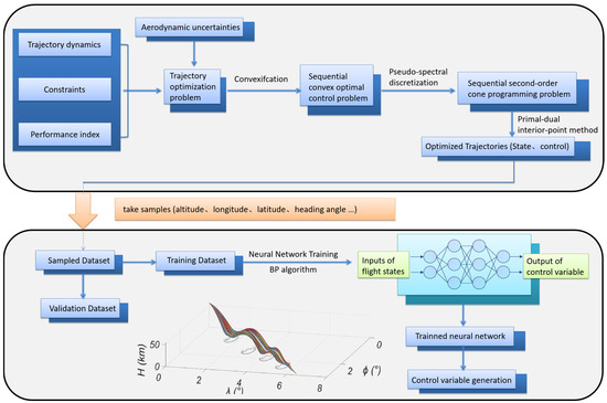
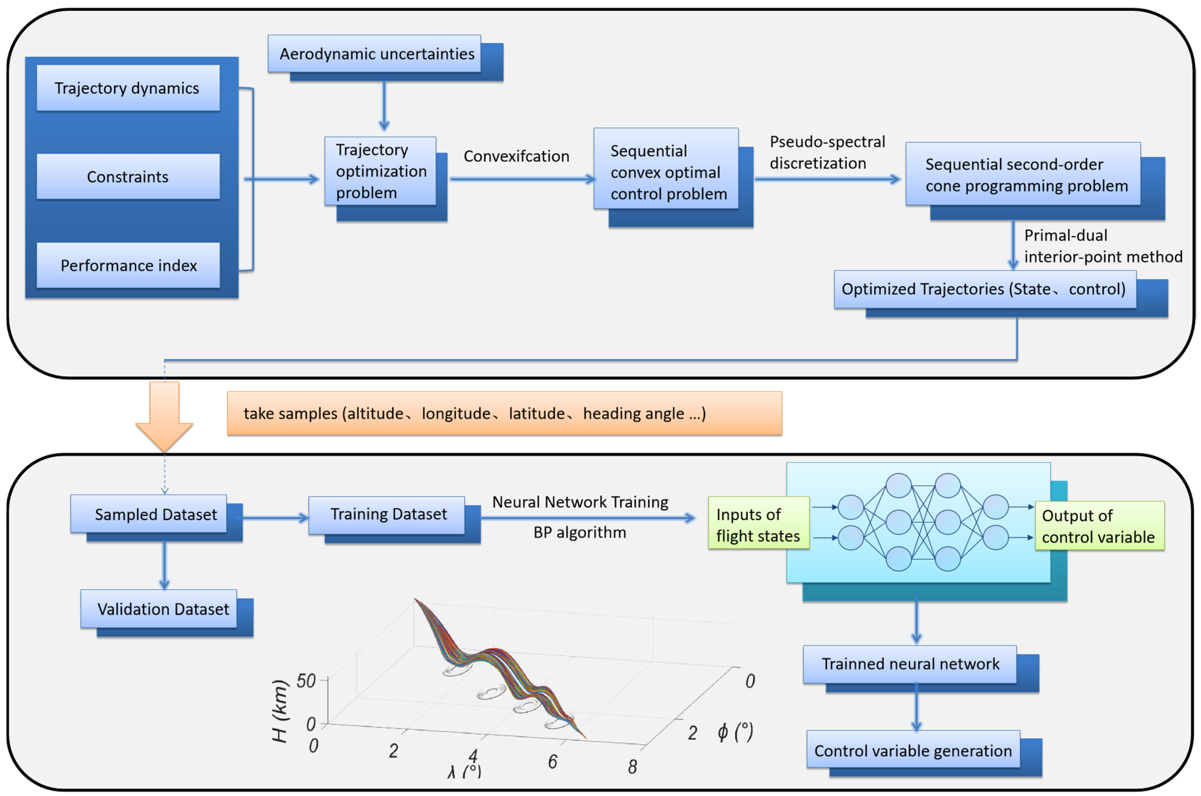
Owing to their universal approximation capability, DNNs efficiently capture complex nonlinear mappings from the input state vector to the optimal control output. After sufficient offline training, the network serves as an embedded controller in the onboard guidance system to generate guidance commands in real time. Because both data sampling and network training are implemented offline, the presented DNN-based approach significantly reduces online computational latency while maintaining high control precision.

Figure 3 shows a schematic of the DNN-based optimal trajectory generation strategy tailored for a morphing gliding reentry vehicle. Within a predefined flight mission profile, the required optimal state-control dataset is generated using the direct method. Following a rigorous dataset preprocessing step, the data are fed into the DNN for offline training. The model learns complex nonlinear mapping in the dataset to predict the optimal control actions of the vehicle based on the flight state feedback. In practical operation, the trained DNN estimates the corresponding optimal control action $u_t$ (i.e., angle of attack ${\alpha }_t$, bank angle ${\sigma }_t$, and sweep angle ${\mathsf{\Lambda }}_t$) by integrating the current input flight state $x_t$ and the NFZ range $(R,x,y)$.

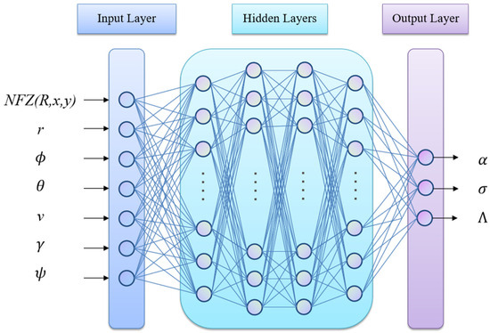
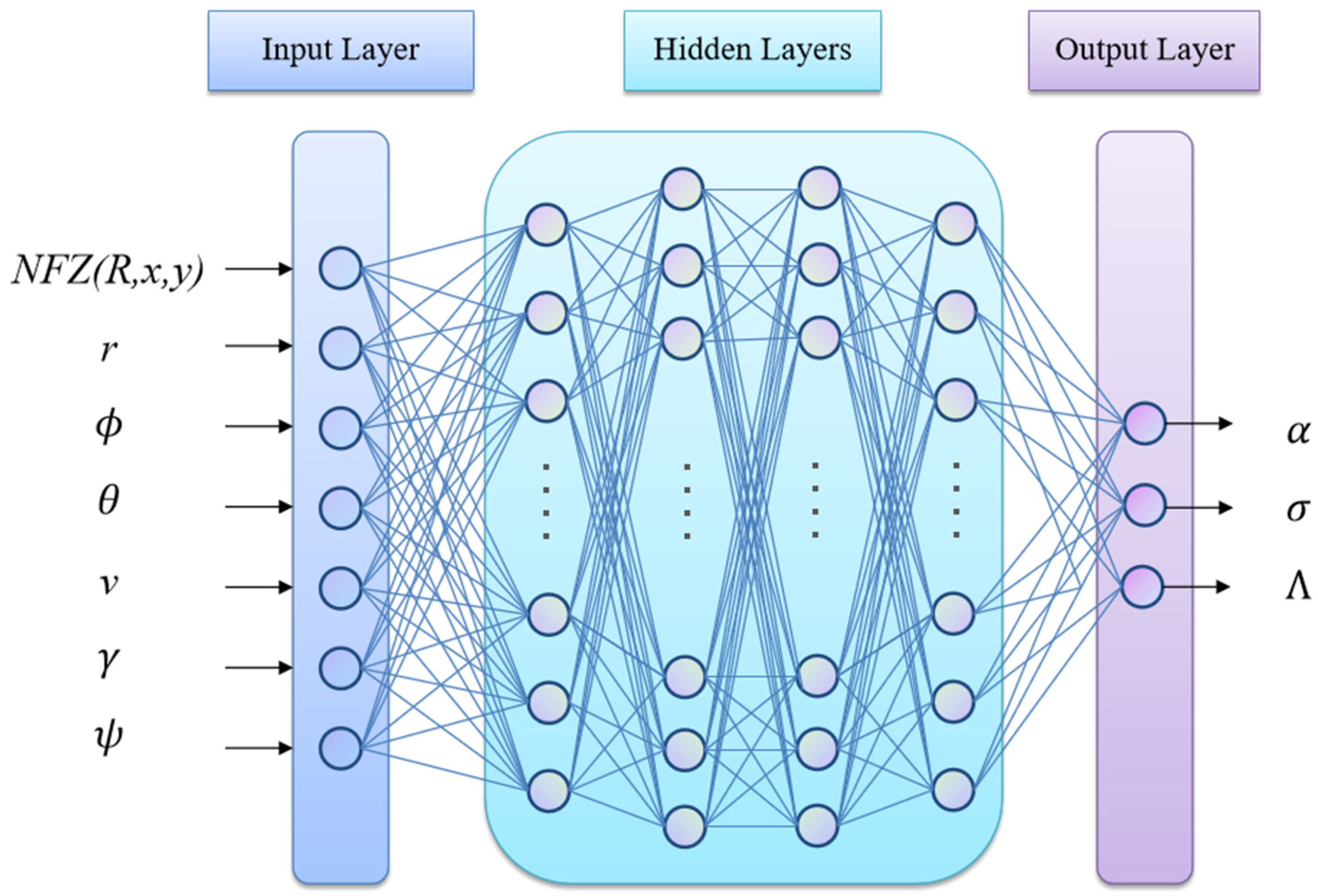
These DNN-based guidance controllers involve two operational paradigms. First, the trained controller can directly generate optimal guidance commands in real time (usually on the millisecond scale) by processing the current flight state feedback. The other system can rapidly generate a complete reference reentry trajectory (typically within seconds) based on specific initial entry conditions. A detailed schematic of the DNN architecture, which explicitly characterizes its inputs, outputs, and topological structure, is shown in Figure 4.

2.4.2. Design and Optimization of DNN

This subsection describes the design of the DNN model and methodology for hyperparameter optimization. A fully connected feedforward neural network comprising a dedicated input layer, series of hidden layers, and final output layer is employed. The network input consists of the state variables of the optimal trajectory, which is composed of $x=[r,\theta ,\varphi ,v,\gamma ,\psi ,\alpha ,\sigma ,\mathsf{\Lambda }]$. During the training process, the DNN learns the intrinsic nonlinear mapping between the state vector and the optimal control actions, $u=[\alpha ,\sigma ,\mathsf{\Lambda }]$. The output $o_{ij}$ corresponding to the ($i$) unit in the ($j$) layer of the network is formulated as

$$o_{ij}=g(w_{ij}{o}_{i-1}+b_{ij})$$

(27)

where $w_{ij}$ designates the weight vector and $b_{ij}$ is the bias vector associated with this unit. Additionally, $O_{(j-1)}$ represents the aggregate output vector derived from the preceding layer and $\phi$ denotes the nonlinear activation function characterizing the unit.

To improve the performance of the optimization algorithm, accelerate the convergence speed, and reduce the computational cost, the altitude and velocity in the input vector are normalized as follows:

$$r_{pre}={\displaystyle \frac{r}{R_e}},v_{pre}={\displaystyle \frac{v}{v(t_0)}}$$

(28)

where $R_e$ denotes the radius of the Earth; $v\left(t_0\right)$ is the initial reentry flight velocity of the vehicle; and $r_{pre}$ and $v_{pre}$ represent the altitude and velocity values, respectively, after preprocessing.

Within the deep learning framework, the loss function $L$ quantifies the divergence between the predicted outputs of the model and actual ground truth labels. This function guides and optimizes the model training, aiming to minimize the loss function to improve the accuracy of the predictions. Owing to its superior robustness against outliers, the mean absolute error (MAE) is selected as the specific loss function. Its definition is presented in Equation (29):

$$L={\displaystyle \frac{1}{N}}{\displaystyle \sum _{i=1}^N|}Net(x_i)-y_i|$$

(29)

where $N$ denotes the total number of training samples; $Net(x_i)$ represents the output predicted by the neural network with the input state vector $x_i$; and $y_i$ denotes the optimization data obtained using the direct method.

The first hyperparameter of a DNN is the network structure, which includes the number of hidden layers and neurons in each layer. An overly simple structure limits the ability of the network to learn nonlinear input–output mapping, resulting in underfitting. Conversely, an excessive number of layers or neurons increases the computational cost and risk of overfitting, where the model performs well on the training set but poorly on the unseen validation data. Accordingly, the final network adopted in this study comprises eight layers with 512 neurons per layer. The hidden-layer activation function is ReLU, and the learning-rate scheduler employs a patience-based strategy with a patience value of 10 and a minimum learning rate of 10⁻⁶. The model weights are updated iteratively using mini-batch gradient descent. Thus, batch size and initial learning rate are another set of essential hyperparameters. The batch size defines the number of samples used in each training iteration and is chosen to balance computational efficiency and gradient stability. Large batch sizes may slow convergence and cause large fluctuations in the validation set, whereas extremely small sizes significantly increase the training time. Therefore, a batch size of 256 is used. The learning rate is the updating step for the network parameters. A low learning rate leads to slow convergence and a long training duration. In contrast, a high learning rate may cause unstable training or convergence to inferior solutions. Therefore, an initial learning rate of 10⁻⁴ is adopted.

All numerical experiments were conducted on a PC with an Intel Core i9-14900HX processor, NVIDIA GeForce RTX 4070 GPU, 32 GB DDR5 RAM, and 1 TB SSD, running the 64-bit Windows 11 operating system. The required software environments including MATLAB 2020 integrated with the CVX toolbox and Python with the PyTorch framework. Detailed hardware specifications, software versions, and key parameter settings are fully documented to ensure the reproducibility of all results presented.

3. Results

3.1. Generation Scheme of Optimal Trajectory Cluster

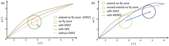
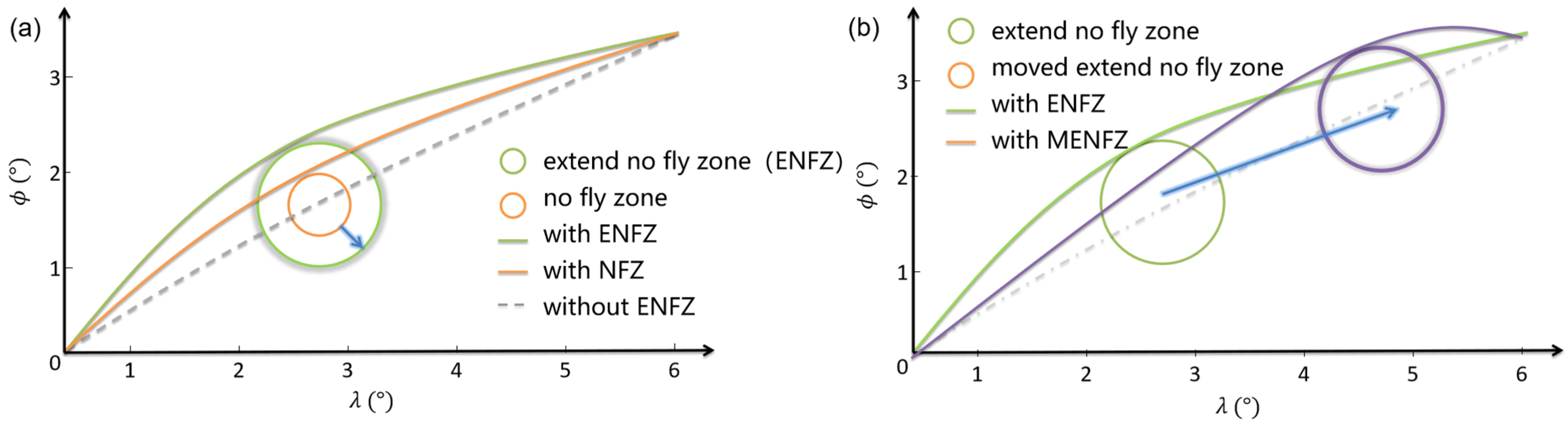
Variable reentry glide vehicles often encounter dynamic NFZs that may shift or expand over time. Therefore, the DNN used as a trajectory generator is designed to adapt to a wide range of NFZ conditions. The simulation environment includes mobile NFZs with variable ranges to validate performance. When the NFZ expands, the vehicle switches from Trajectory 1 (orange) to Trajectory 2 (green), as shown in Figure 5a. The spatial translation of the NFZ changes from Trajectory 2 (green) to Trajectory 3 (purple), as illustrated in Figure 5b.

To ensure that the dataset covers the broadest possible range of spatial configurations, 2500 NFZs with different positions and sizes were set up in the experiment. The central positions and radius ranges of each NFZ are listed in

Table 2. Range of initial state values for NFZ.

Center of No-Fly Zone	Range of the No-Fly Zone (km)
[1.6, 0.7]	[11.1, 33.3]
[3.0, 1.5]	[11.1, 33.3]
[4.2, 1.9]	[11.1, 33.3]
[5.4, 2.4]	[11.1, 33.3]

.

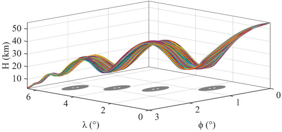
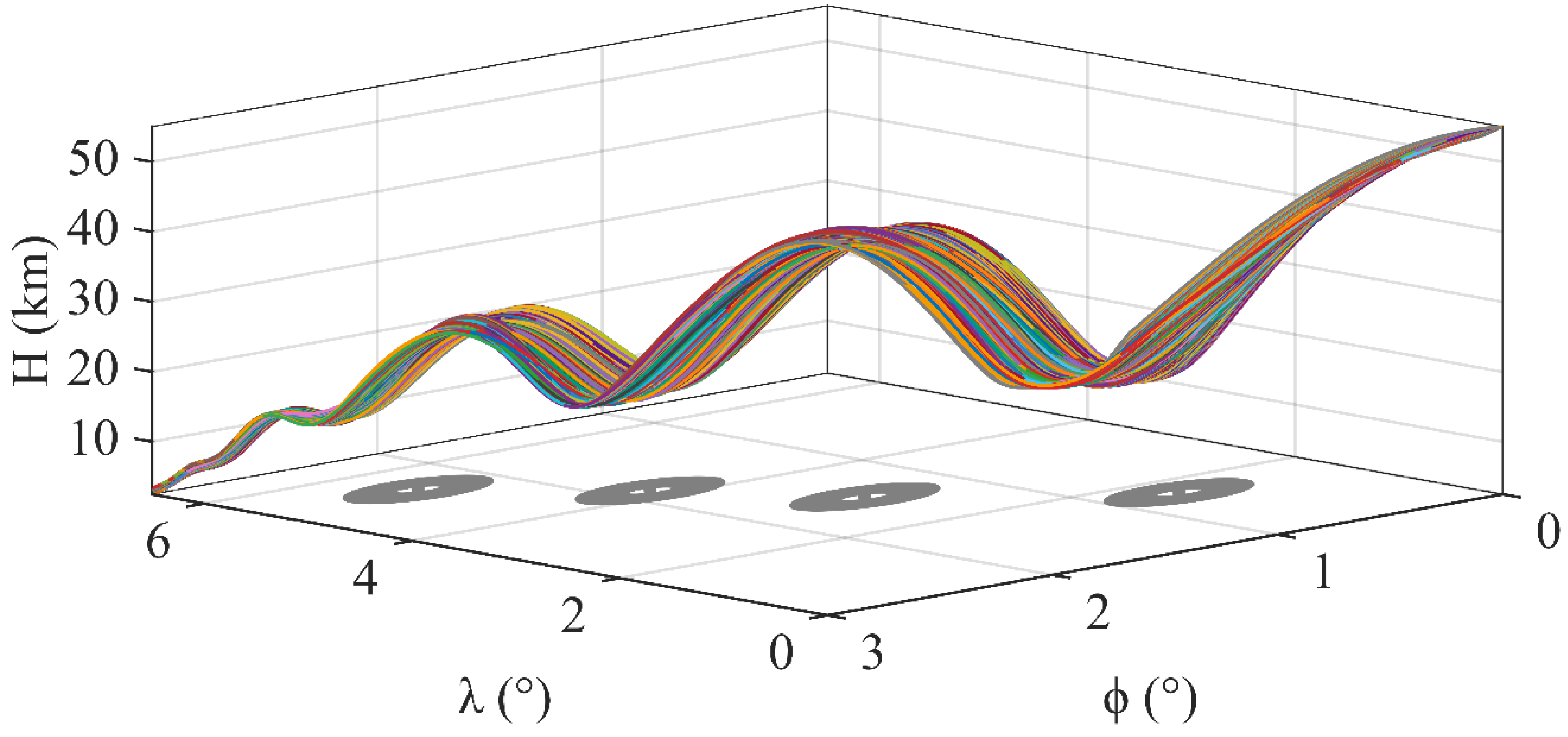
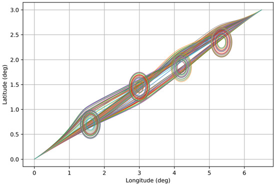
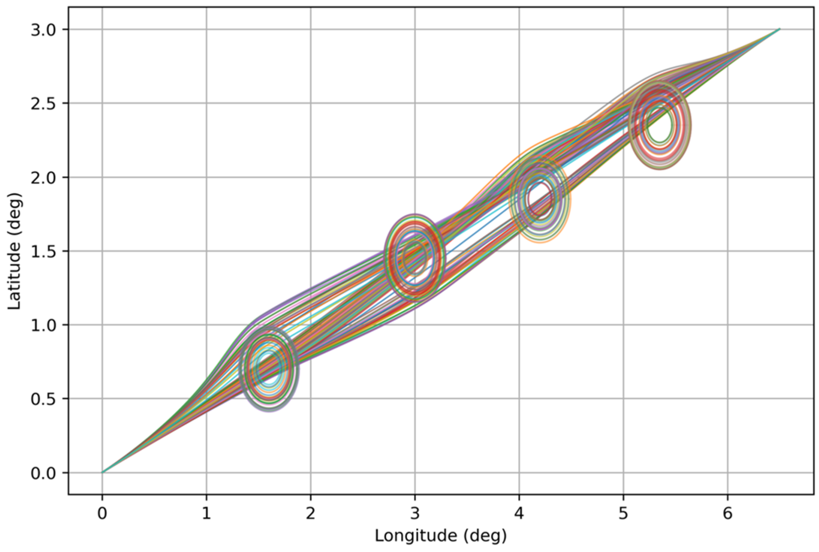
Figure 6 presents the optimal trajectory clusters for variable gliding reentry vehicles under different NFZ configurations. These clusters cover all scenarios where the NFZ shifts among the four NFZ centers and its range varies from 11.1 km to 33.3 km.

3.2. Parameter Settings of Radau Pseudospectral Convex Optimization

In this study, the Radau pseudospectral convex optimization method was employed to generate an optimal trajectory library. The number of Gaussian collocation points per trajectory is a key influencing factor in numerical trajectory computation. Insufficient collocation points degrade the quality of trajectory optimization, whereas an excessive number substantially increases the time cost for both trajectory generation and subsequent network training. For the specific scenario investigated in this study, a 2 s interval between collocation points ensures sufficient trajectory accuracy. The reentry flight duration is about 700 s. After balancing the generation time and optimization quality, each trajectory contains approximately 250 discrete optimal state-action sets on average. This setup generates reliable trajectories within acceptable time limits. Although using more Gaussian collocation points is feasible, the time cost increases considerably. The currently selected discretization points guarantee trajectory reliability, and the 2500 samples are divided into 2000 training, 300 validation, and 200 test trajectories.

As shown in

Table 3. Statistical confidence bounds of test-set metrics.

Control Variable	RMSE	95% CI	MAE
Angle of attack	0.239 ± 0.168	[0.215, 0.264]	0.099 ± 0.052
Bank angle	0.107 ± 0.064	[0.098, 0.117]	0.073 ± 0.034
Wing sweep angle	0.462 ± 0.530	[0.385, 0.539]	0.319 ± 0.387

, the DNN model is evaluated on 200 independent test trajectories. Three error metrics are adopted to assess the prediction performance. RMSE reflects the overall prediction error and is sensitive to large local deviations. MAE denotes the average prediction bias. Mean ± std and 95% confidence intervals (CI) are calculated from all valid trajectories to quantify error dispersion and statistical reliability. The model yields stable predictions for angle of attack, bank angle, and sweep angle. The corresponding RMSE values are 0.239, 0.107, and 0.462, with 95% CIs of [0.215, 0.264], [0.098, 0.117], and [0.385, 0.539], respectively. The relatively higher error of sweep angle is mainly caused by a small number of extreme trajectories. For most test cases, the prediction accuracy remains acceptable.

In the simulation, the initial downrange, initial reentry altitude, and initial velocity of the reentry mission are 796.6 km, 55 km, and 2150 m/s, respectively. The bank angle rate is limited to 10°/s.

Table 4. Range of initial state values for trajectories.

Parameter	Value Range
Initial altitude $\mathit{r}$(t0)	55 km
Initial longitude $\mathit{\theta }$(t0)	0°
Initial latitude $\mathit{\varphi }$(t0)	0°
Initial velocity V (t0)	2150 m/s
Initial flight path angle $\mathit{\gamma }$(t0)	66°
Initial Azimuth $\mathit{\psi }$(t0)	−0.5°

lists the bank angle bounds and path constraint limits.

For the two examples investigated in this section, the parameter settings of the trust region size and convergence criterion are given by Equations (30) and (31), respectively, as follows:

$$\delta ={\left[{\displaystyle \frac{10000}{R_0}},{\displaystyle \frac{20\pi }{180}},{\displaystyle \frac{20\pi }{180}},{\displaystyle \frac{500}{V_0}},{\displaystyle \frac{20\pi }{180}},{\displaystyle \frac{20\pi }{180}},{\displaystyle \frac{20\pi }{180}}\right]}^T$$

(30)

$$\epsilon ={\left[{\displaystyle \frac{100}{R_0}},{\displaystyle \frac{0.05\pi }{180}},{\displaystyle \frac{0.05\pi }{180}},{\displaystyle \frac{1}{V_0}},{\displaystyle \frac{0.05\pi }{180}},{\displaystyle \frac{0.05\pi }{180}},{\displaystyle \frac{1\pi }{180}}\right]}^T$$

(31)

To verify the rationality and robustness of the parameter configuration in the proposed SCP algorithm, single-factor sensitivity analysis is performed on parameters $\rho$, ${\lambda }_1$, and ${\lambda }_2$. The default values are set as ${\rho }_0={10}^{-2}$, ${\lambda }_1={10}^2$, and ${\lambda }_2={10}^1$. In each test, only one parameter is modified, while the rest remain at default settings. Several key indicators are adopted for quantitative evaluation, including solution success rate, average iteration number, average computation time, and maximum path constraint violation. Test results show that all parameter groups achieve a 100% success rate in solving convex subproblems. The parameter $\rho$ primarily governs algorithm convergence. A small $\rho$ value increases the reliance on virtual controls, while an excessively large value raises the difficulty of numerical computation. ${\lambda }_1$ mainly determines terminal position accuracy, and ${\lambda }_2$ has limited impacts within the test range. The default parameters adopted in this work effectively balance terminal accuracy, path constraint satisfaction, virtual control suppression, and computational efficiency.

For the sequential convex programming (SCP) method, $\rho$ is the most sensitive parameter for convergence performance. A smaller $\rho$ relaxes dynamic consistency constraints, whereas a larger $\rho$ complicates numerical solving. The default ${\rho }_0$ lies in a reasonable range, which well balances virtual control suppression, terminal precision and computational cost. ${\lambda }_1$ barely affects solution feasibility but significantly influences terminal position accuracy. A larger ${\lambda }_1$ can reduce terminal errors, accompanied by a slight increase in computational burden. Within the test scope, ${\lambda }_2$ exerts negligible influences on SCP solution stability, which verifies the good parameter robustness of the proposed algorithm, as shown in

Table 5. SCP optimization performance with varying parameter magnitudes.

Parameter Perturbation	Success Rate of Solution	Average Iterations	Average Time	Terminal Error Mean Range
ρ = 0.1ρ0~10ρ0	100%	2.5–4.3	29.9–59.9 s	3.99 × 10−7–4.21 × 10−3
λ1 = 0.1λ10~10λ10	100%	3.3–4.0	38.7–52.9 s	1.40 × 10−3–4.30 × 10−3
λ2 = 0.1λ20~10λ20	100%	3.6–3.9	47.5–52.5 s	2.91 × 10−3–3.97 × 10−3

.

To further explore the convergence characteristics and anti-disturbance capability of the SCP algorithm, this paper investigates its robustness against perturbed initial reference trajectories. Four trajectory levels with different perturbation magnitudes are established, including nominal, small, moderate, and large perturbation trajectories. All perturbations are imposed only on the reference trajectory for SCP linearization, while the practical boundary conditions and path constraints are fixed during all tests.

The test results shown in

Table 6. Quantitative performance under different initial reference trajectory perturbations.

Initial Reference	Solver Success	Mean SCP Iterations	Mean Terminal Error
Nominal	100%	1.2	6.5 × 10−5
Small perturbation	65%	5.0	5.5 × 10−5
Medium perturbation	5%	5.0	6.2 × 10−5
Large perturbation	0%	—	—

verify that the SCP algorithm converges stably when the reference trajectory is close to the feasible domain. All test cases converge successfully under nominal trajectories, achieving a 100% core state convergence rate. For small perturbation scenarios, the solution success rate decreases to 65%. Most convergent cases reach the maximum iteration number, but their terminal errors and path constraints still meet the requirements. Only 5% of test cases converge under moderate perturbations, with a sharp rise in virtual control norm. No effective solutions can be obtained when large perturbations are applied. These results confirm the local convergence feature of the SCP algorithm. A reference trajectory close to the feasible domain guarantees stable optimization performance. In contrast, trajectories far from the feasible domain cause severe convexification errors. These errors reduce solution accuracy and success rate, raise iteration costs and virtual control amplitude. In extreme perturbation scenarios, the convex subproblems fail to generate feasible solutions.

3.3. Generation Results of Training and Testing Data

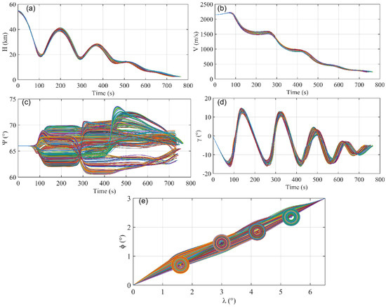
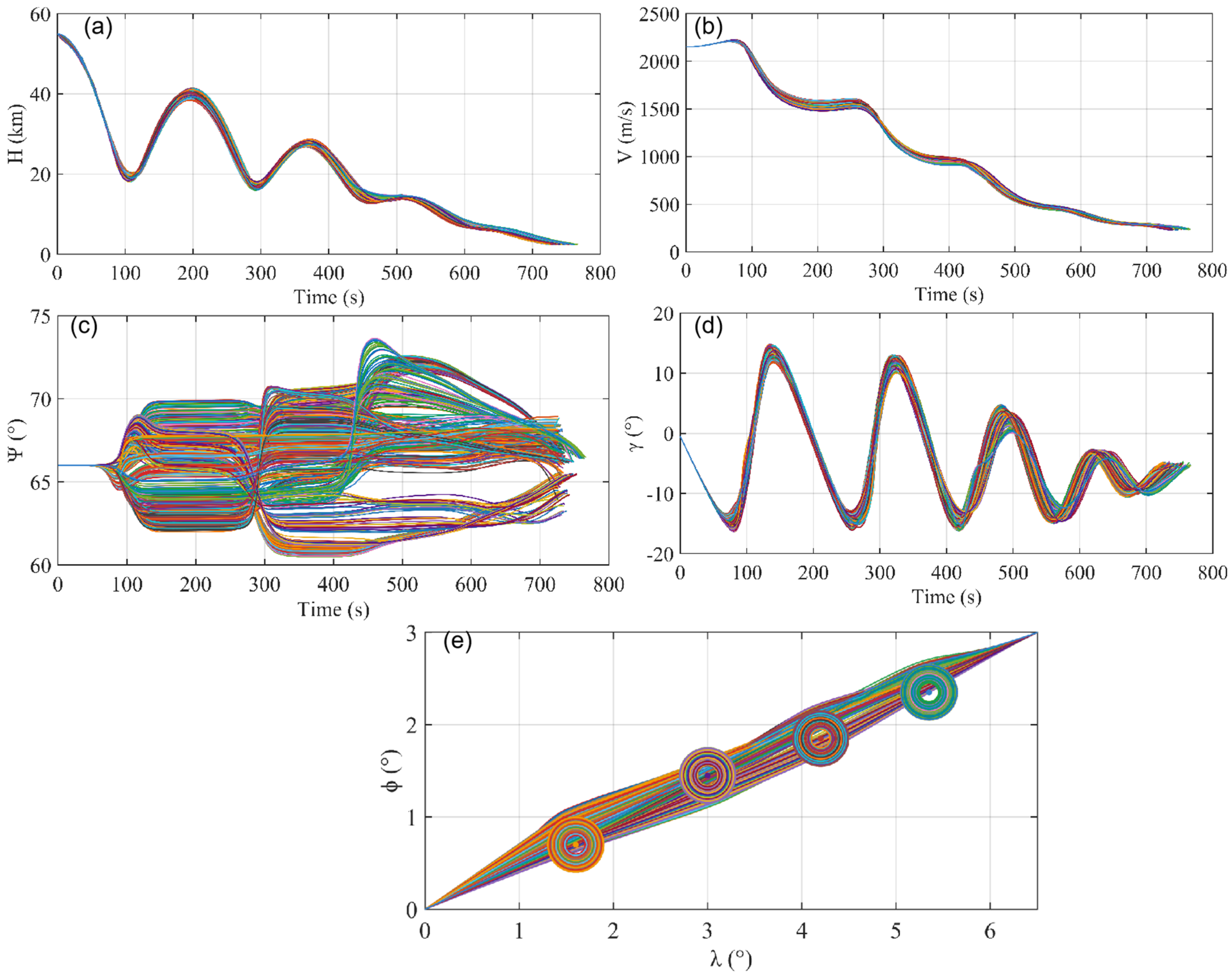
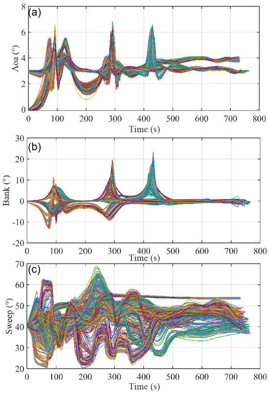
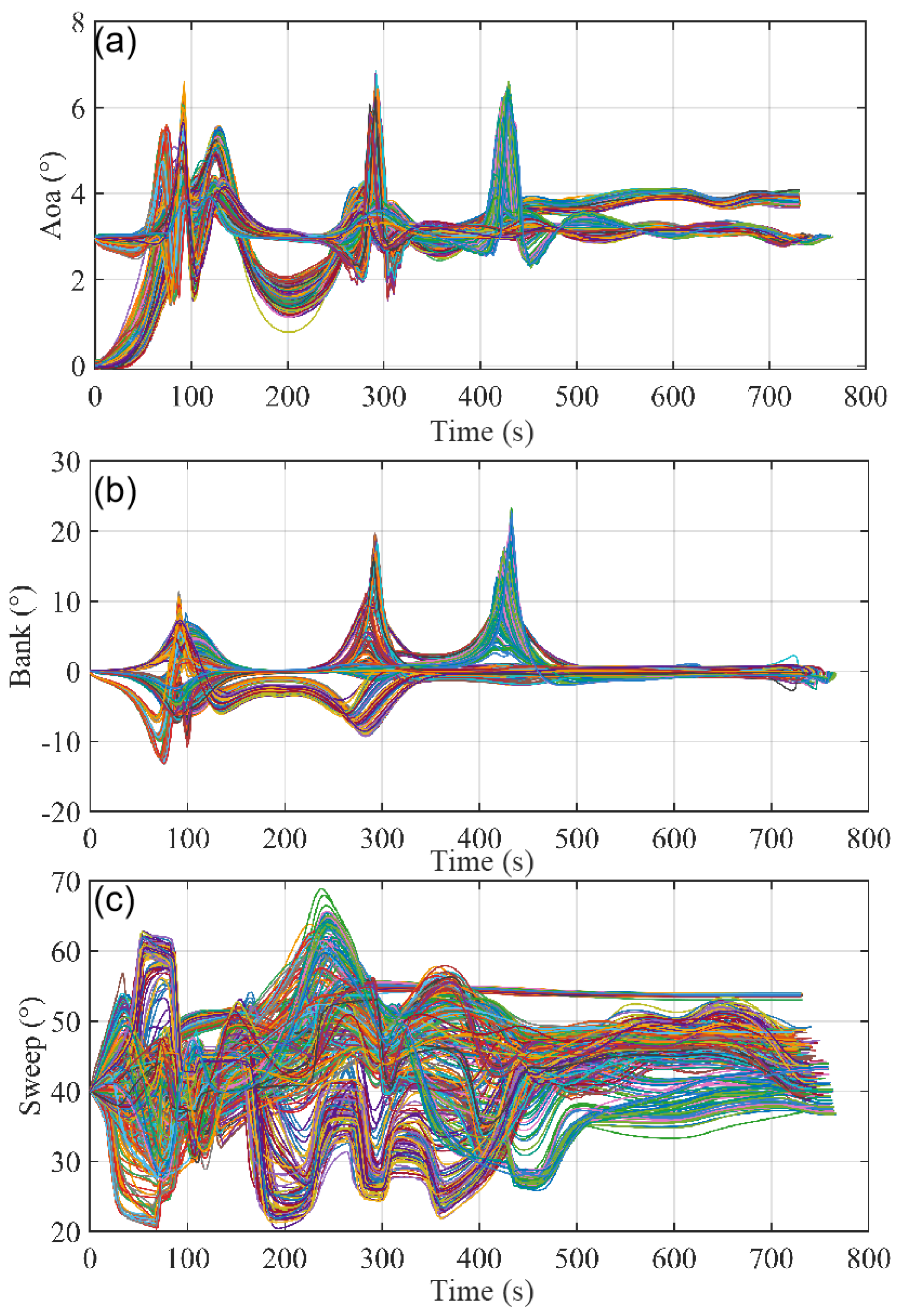
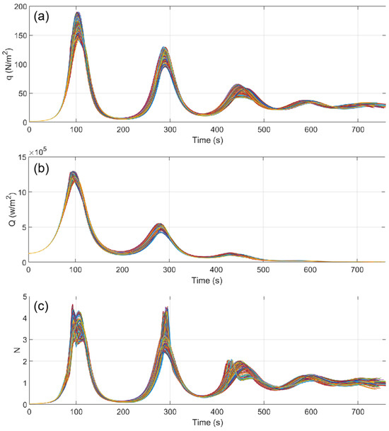
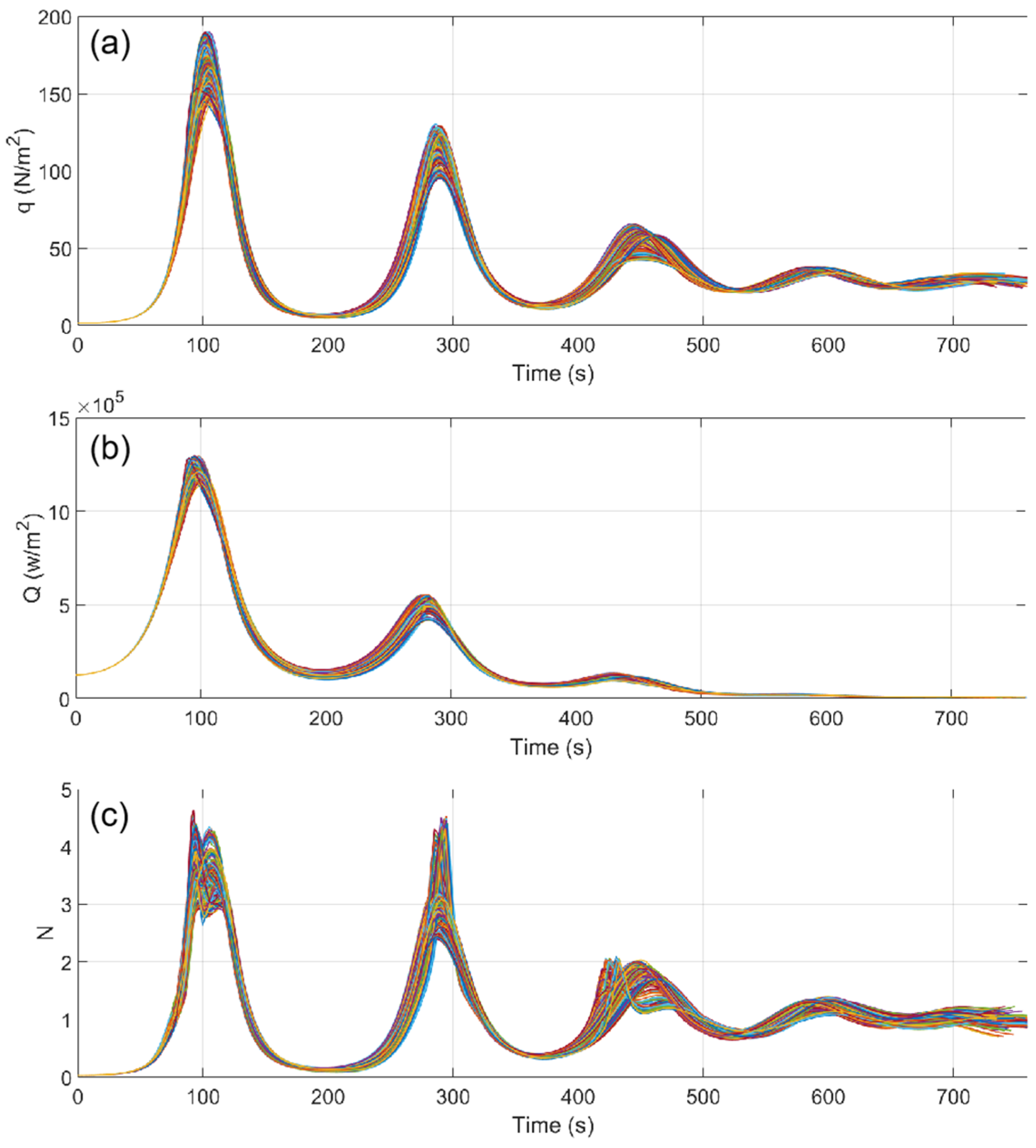
Figure 7a shows 2500 optimal trajectories under random NFZs. The constraints of the heat flux, dynamic pressure, and overload are shown in Figure 8, with the maximum heat flux appearing at the start of gliding. To satisfy the heat-flux constraint, the vehicle adjusts the wing sweep angle to generate lift for trajectory pull-up, thereby reducing energy loss and severe aerothermal environments from high-angle-of-attack flights. Figure 7c illustrates the variation in the bank angle. For a safe flight and large-scale lateral maneuvering, the bank angle is adjusted several times during the mission. Figure 9 shows the variation in the wing sweep angle. The deformation results show that the sweep angle coordinates with the attitude angle during large-scale lateral maneuvers. The angle of attack remains within a narrow range throughout the flight, which benefits gliding range extension and thermal protection design.

3.4. Neural Network Prediction Results

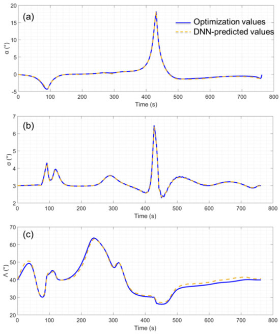
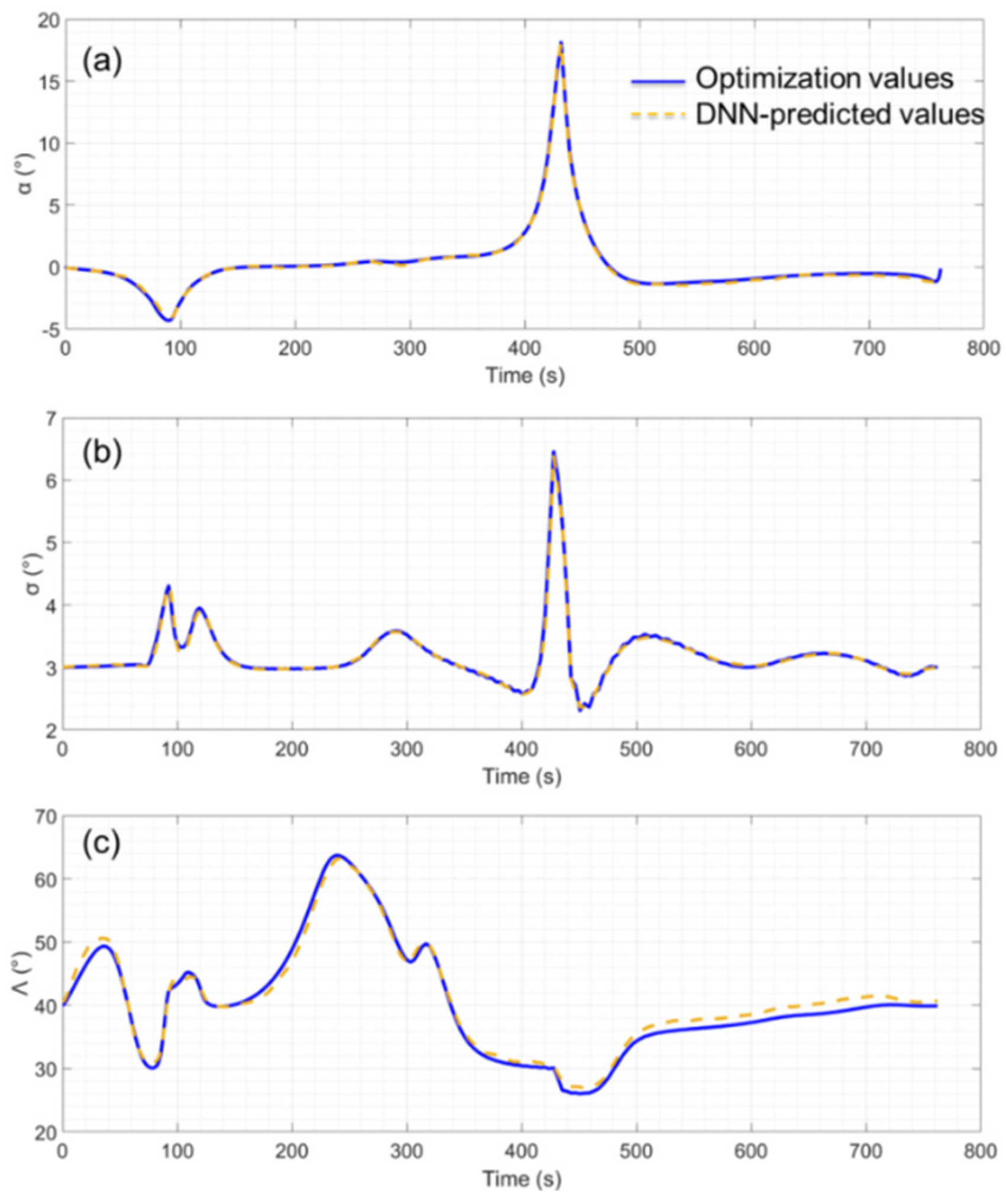
To further verify the performance of the proposed DNN, the trained model uses the current flight state vector to generate predictions and provides control inputs (angle of attack α, bank angle σ, and sweep angle Λ) at the corresponding time. Figure 10 compares a trajectory randomly selected from the network validation dataset with that predicted by the neural network. The results demonstrate that the proposed neural network accurately predicts trajectories based on the current flight state.

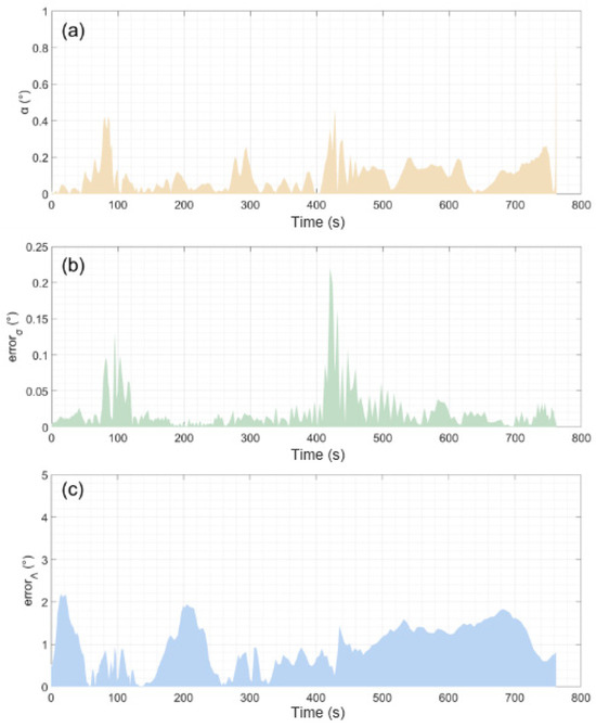
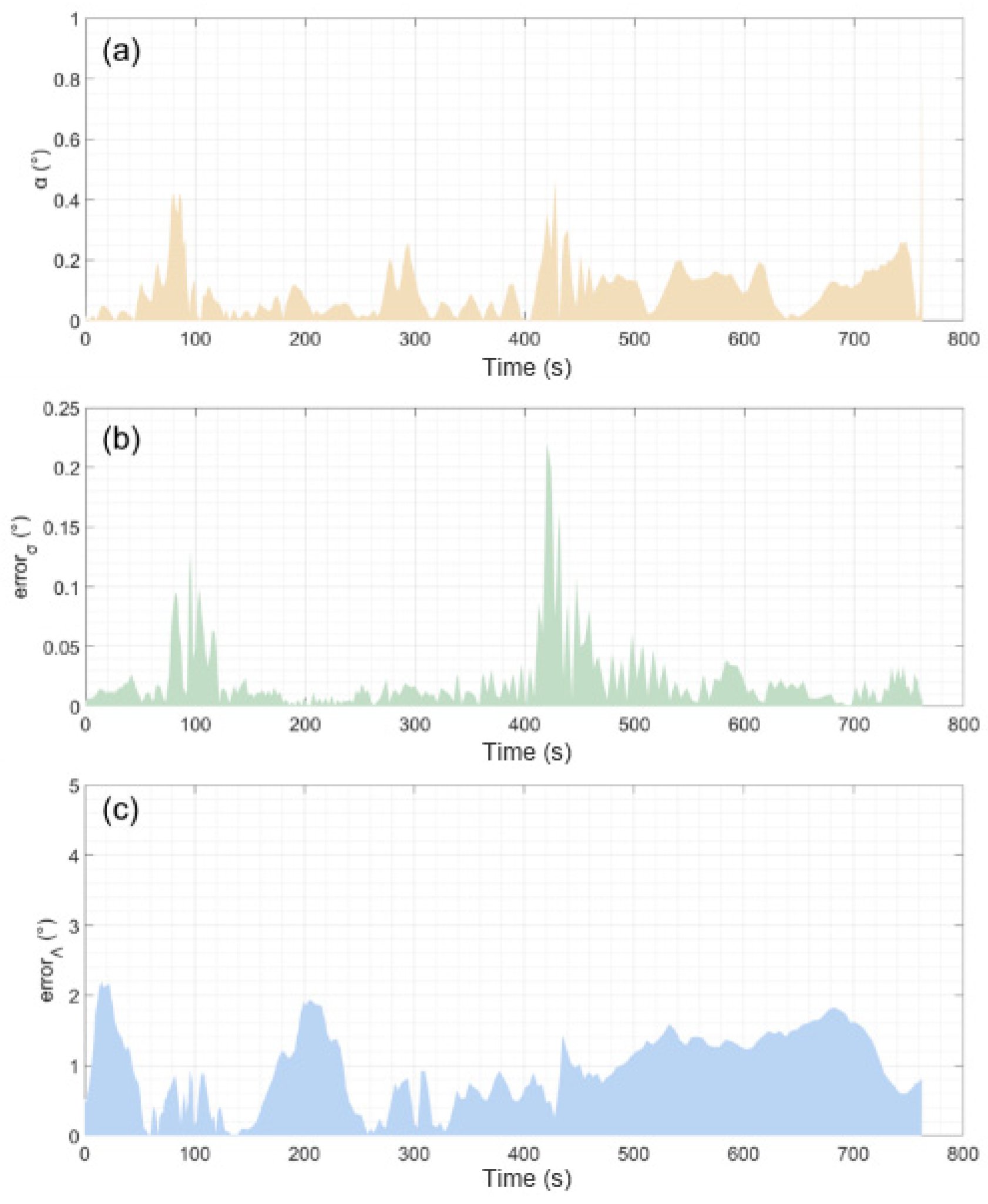
Figure 11 shows the absolute error distribution of the optimal actions predicted by the neural network. Analysis reveals that the angle of attack α has an average relative error of 2.25% and an absolute error of 0.912°; the bank angle σ has a relative error of 0.61% and an absolute error of 0.02°; the wing sweep angle Λ has a relative error of 2.25% and an absolute error of 0.912°. The designed DNN model demonstrates high accuracy in predicting optimal actions, thereby facilitating precise real-time guidance (only 0.4 ms is required to predict three groups of control variables).

To verify the effectiveness of the proposed algorithm, 200 trajectory cases are tested via Monte Carlo experiments, as presented in Figure 12. Diverse initial flight states are employed to produce validation trajectories, whose key parameters are summarized in

Table 7. Range of state values for Monte Carlo experiments.

Parameter	Value Range
Initial altitude $\mathbf{r}$	55 ± 0.5 km
No-fly zone radius range	The no-fly zone radius is randomly chosen between 0.10° and 0.30°.
Initial velocity V	2150 ± 20 m/s
Initial flight path angle $\mathsf{\gamma }$(t0)	66 ± 0.5°
Initial Azimuth $\mathsf{\psi }$(t0)	−0.5 ± 1°

. The average terminal position error, altitude error, and velocity error are measured as 12.85 km, 1.02 km, and 70.87 m/s correspondingly. It is shown that the DNN method delivers satisfactory terminal tracking accuracy and satisfies the requirements imposed by strong path constraints.

4. Discussion

This study proposes an online trajectory co-optimization framework for morphing gliding reentry vehicles, which integrates deep neural networks (DNNs) with sequential Radau pseudospectral convex optimization methods. The established framework transforms the strongly non-convex trajectory planning problem with complex flight constraints into a series of tractable convex subproblems. Specifically, DNNs are employed to construct the nonlinear mapping between flight state parameters and optimal control variables, forming a hybrid optimization paradigm that combines high-precision numerical optimization and rapid intelligent inference. This strategy enables the real-time generation of optimal flight trajectories and synchronous wing morphing strategies throughout the full flight envelope, and exhibits excellent adaptability to complex flight missions involving dynamic no-fly zone constraints and time-varying range limitations.

Despite the promising performance of the developed framework in nominal flight scenarios, several inherent limitations restrict its practical engineering application. First, the training dataset of the DNN model is limited to conventional flight envelopes and common disturbance conditions, lacking coverage of extreme working scenarios. Abrupt variations in no-fly zone boundaries and intense external disturbances will degrade the model inference accuracy, and may further lead to the failure of trajectory optimization. Perturbation simulation experiments verify the local convergence characteristic of the adopted SCP algorithm. The algorithm can achieve complete convergence when the initial reference trajectory is close to the feasible solution domain. Nevertheless, small trajectory perturbations reduce the solution success rate to 65%, even though the convergent solutions still meet the basic accuracy and constraint requirements. Severe trajectory perturbations will completely invalidate the optimization results and fail to generate feasible flight trajectories. Second, the SCP algorithm relies on linearization and convex relaxation operations to approximate the original non-convex flight constraints. Such numerical approximation operations will inevitably introduce minor systematic errors, especially under extreme boundary constraint conditions. For flight missions with extremely narrow safety margins, these approximation errors make it difficult for the framework to guarantee the strict global optimality of the optimized trajectory and morphing strategies.

Future research will focus on addressing the aforementioned limitations to further improve the generalization performance and engineering practicability of the proposed framework. First, extended datasets containing diverse extreme flight scenarios and drastic constraint variation cases will be supplemented to expand the adaptive boundary of the DNN model, so as to enhance the robustness of intelligent inference against severe disturbances and abrupt mission changes. Second, adaptive convex relaxation strategies and dynamic error correction algorithms will be developed to compensate the linearization errors of SCP, thereby improving the optimization accuracy under boundary-limited flight conditions. Third, high-fidelity flight perturbation factors including aerodynamic uncertainty, sensor measurement noise and actuator execution deviation will be incorporated to construct a simulation platform that is highly consistent with real flight environments. Furthermore, online parameter updating and incremental learning mechanisms will be explored to realize adaptive adjustment of the framework for unknown and complex mission scenarios. This work provides a solid theoretical and technical foundation for the engineering implementation of online intelligent co-optimization of trajectories and morphing strategies for morphing reentry vehicles.

References

- Phoenix, A.; Rogers, R.E.; Maxwell, J.R.; Goodwin, G.B. Mach five to ten morphing waverider: Control point study. J. Aircr. 2019, 56, 493–504. [Google Scholar] [CrossRef] [Scilit]
- Bowcutt, K. Hypersonic Waverider Variable Leading Edge Flaps. U.S. Patent US6634594B1, 21 October 2003. [Google Scholar]
- Maxwell, J.R. Hypersonic waverider stream surface actuation for variable design point operation. In Proceedings of the 52nd AIAA/SAE/ASEE Joint Propulsion Conference, Salt Lake City, UT, USA, 25–27 July 2016; p. 4706. [Google Scholar]
- Phoenix, A.; Maxwell, J.R.; Goodwin, G.B. Morphing high-temperature surfaces for shape control hypersonic waverider vehicles. In Proceedings of the Modeling, Simulation, Control & Adaptive Systems Design and Implementation, Structural Health Monitoring, Snowbird, UT, USA, 18–20 September 2017; pp. 1–5. [Google Scholar]
- Xie, Y.; Liu, L.; Tang, G.; Zheng, W. A reentry trajectory planning approach satisfying waypoint and no-fly zone constraints. In Proceedings of the 5th IEEE International Conference on Recent Advances in Space Technologies (RAST), Istanbul, Turkey, 9–11 June 2011; pp. 241–246. [Google Scholar]
- Ottesen, D.; Russell, R.P. Direct-to-indirect mapping for optimal low-thrust trajectories. Astrodynamics 2024, 8, 27–46. [Google Scholar]
- Xue, S.; Ping, L. Constrained Predictor-Corrector Entry Guidance. J. Guid. Control Dyn. 2010, 33, 1273–1281. [Google Scholar] [CrossRef] [Scilit]
- Zhang, J.; Liu, K.; Fan, Y.; She, Z. A Piecewise Predictor-corrector Reentry Guidance Algorithm with No-fly Zone Avoidance. J. Astronaut. 2021, 42, 122–131. [Google Scholar]
- Li, M.; Zhou, C.; Shao, L.; Lei, H.; Luo, C. An Improved Predictor-Corrector Guidance Algorithm for Reentry Glide Vehicle Based on Intelligent Flight Range Prediction and Adaptive Crossrange Corridor. Int. J. Aerosp. Eng. 2022, 2022, 731586. [Google Scholar] [CrossRef] [Scilit]
- Yong, E.M.; Qian, W.Q.; He, K.F. An adaptive predictor-corrector reentry guidance based on self-definition way-points. Aerosp. Sci. Technol. 2014, 39, 221–225. [Google Scholar] [CrossRef] [Scilit]
- Zhu, J.; Liu, L.; Tang, G.; Bao, W. Highly constrained optimal gliding guidance. Proc. Inst. Mech. Eng. Part G J. Aerosp. Eng. 2015, 229, 2321–2335. [Google Scholar] [CrossRef] [Scilit]
- Liu, X.; Lu, P. Survey of convex optimization for aerospace applications. Astrodynamics 2017, 1, 23–40. [Google Scholar] [CrossRef] [Scilit]
- Liu, X.; Shen, Z.; Lu, P. Entry trajectory optimization by second-order cone programming. J. Guid. Control Dyn. 2016, 39, 227–241. [Google Scholar] [CrossRef] [Scilit]
- Wang, Z.; Grant, M.J. Constrained trajectory optimization for planetary entry via sequential convex programming. J. Guid. Control Dyn. 2017, 40, 2603–2615. [Google Scholar] [CrossRef] [Scilit]
- Wang, Z.; Grant, M.J. Autonomous entry guidance for hypersonic vehicles by convex optimization. J. Spacecr. Rocket. 2018, 55, 993–1006. [Google Scholar] [CrossRef] [Scilit]
- Sandberg, A.; Sands, T. Autonomous trajectory generation algorithms for spacecraft slew maneuvers. Aerospace 2022, 9, 135. [Google Scholar] [CrossRef] [Scilit]
- Rozza, G.; Sands, T. Autonomous trajectory generation comparison for de-orbiting with multiple collision avoidance. Sensors 2022, 22, 7066. [Google Scholar] [CrossRef] [Scilit]
- Wang, J.; Cui, N.; Wei, C. Rapid trajectory optimization for hypersonic entry using convex optimization and pseudospectral method. Aircr. Eng. Aerosp. Technol. 2019, 91, 669–679. [Google Scholar] [CrossRef] [Scilit]
- Liu, X.; Li, S.; Xin, M. Mars Entry Trajectory Planning with Range Discretization and Successive Convexification. J. Guid. Control Dyn. 2022, 45, 755–763. [Google Scholar] [CrossRef] [Scilit]
- Li, S.; Liu, X.; Jiang, X.-Q.; Peng, Y.-M. Trajectory Optimization and Guidance Methods for Mars Entry; Springer: Singapore, 2024. [Google Scholar]
- Liu, X.; Li, S. Survey of Trajectory Optimization Methods for Mars Entry and Powered Descent. J. Guid. Control Dyn. 2026, 49. [Google Scholar] [CrossRef] [Scilit]
- Wang, Z.; Zhang, H. Improved sequential convex programming algorithms for entry trajectory optimization. J. Spacecr. Rocket. 2020, 57, 1373–1386. [Google Scholar] [CrossRef] [Scilit]
- Zhou, X.; He, R.; Zhang, H.; Tang, G.; Bao, W. Sequential convex programming method using adaptive mesh refinement for entry trajectory planning problem. J. Astronaut. Technol. 2021, 109, 106374. [Google Scholar] [CrossRef] [Scilit]
- Zhou, X.; Zhang, H.B.; Xie, L.; Tang, G.J.; Bao, W.M. An improved solution method via the pole-transformation process for the maximum-endurance problem. Proc. Inst. Mech. Eng. Part G J. Aerosp. Eng. 2020, 234, 1941–1956. [Google Scholar]
- Liu, X.; Shen, Z.; Lu, P. Exact convex relaxation for optimal flight of aerodynamically controlled missiles. IEEE Trans. Aerosp. Electron. Syst. 2019, 55, 1881–1892. [Google Scholar]
- Izzo, D.; Martens, M.; Pan, B. A Survey on Artificial Intelligence Trends in Spacecraft Guidance Dynamics and Control. Astrodynamics 2019, 3, 287–299. [Google Scholar] [CrossRef] [Scilit]
- Sanchez-Sanchez, C.; Izzo, D. Learning the Optimal State-Feedback Using Deep Networks. In Proceedings of the IEEE Symposium Series on Computational Intelligence (SSCI), Athens, Greece, 6–9 December 2016. [Google Scholar]
- Izzo, D.; Sprague, C.; Tailor, D. Machine Learning and Evolutionary Techniques in Interplanetary Trajectory Design. arXiv 2018, arXiv:1802.00180. [Google Scholar]
- Sanchez-Sanchez, C.; Izzo, D. Real-Time Optimal Control via Deep Neural Networks: Study on Landing Problems. J. Guid. Control Dyn. 2018, 41, 1122–1135. [Google Scholar] [CrossRef] [Scilit]
- Li, H.; Chen, H.; Tan, C.; Jiang, Z.; Xu, X. Fast Trajectory Generation with a Deep Neural Network for Hypersonic Entry Flight. Aerospace 2023, 10, 931. [Google Scholar] [CrossRef] [Scilit]
- Dai, P.; Yan, B.; Huang, W.; Zhen, Y.; Wang, M.; Liu, S. Design and aerodynamic performance analysis of a variable-sweep-wing morphing waverider. Aerosp. Sci. Technol. 2020, 98, 105703. [Google Scholar] [CrossRef] [Scilit]
- Dai, P.; Yan, B.; Liu, R.; Liu, S.; Wang, M. Integrated Morphing Strategy and Trajectory Optimization of a Morphing Waverider and Its Online Implementation Based on the Neural Network. IEEE Access 2021, 99, 59383–59393. [Google Scholar] [CrossRef] [Scilit]
Disclaimer/Publisher’s Note: The statements, opinions and data contained in all publications are solely those of the individual author(s) and contributor(s) and not of MDPI and/or the editor(s). MDPI and/or the editor(s) disclaim responsibility for any injury to people or property resulting from any ideas, methods, instructions or products referred to in the content. |
© 2026 by the authors. Licensee MDPI, Basel, Switzerland. This article is an open access article distributed under the terms and conditions of the Creative Commons Attribution (CC BY) license.