Fast Prediction Model of Infrared Signatures for Vacuum Rocket Plumes

Abstract

Infrared radiation spectra produced by vibration–rotation transitions in multicomponent gases within the vacuum plume of attitude and orbital control engines constitute crucial radiation sources for optical target identification and space maneuver recognition, and rapid prediction of these signatures is essential for real-time forecasting. This study introduces an axisymmetric vacuum plume flow field model based on a simplified point-source approach that accommodates multicomponent combustion gases. Using the Maxwellian velocity distribution and a velocity–position angle algorithm, normalized number density, velocity, and temperature distributions are derived. A plume–freestream interaction model founded on noncentral fully elastic collision theory is incorporated, and overall plume properties are obtained via density-weighted averaging. Neglecting non-equilibrium radiation effects, the high-temperature gas absorption coefficient is calculated using a statistical narrowband model and radiative transfer is solved via the line-of-sight method. The model is validated against direct simulation Monte Carlo results for single-gas and MBB bipropellant plumes and confirmed using infrared spectral data in the 2.0–4.5 μm band. The proposed framework achieves 10²–10³-fold higher computational efficiency than conventional DSMC approaches. Freestream effects on plume diffusion and momentum exchange diminish with increasing altitude, as does the freestream velocity’s enhancement of radiation intensity, whereas greater plume expansion at higher altitudes increases overall radiation intensity.

1. Introduction

Attitude and orbital control thrusters expel high-temperature, high-velocity exhaust gases supersonically into high-altitude or vacuum environments. In such environments, where atmospheric molecular density is extremely low and mean free paths exceed 10 m [1], engine exhaust forms a highly under-expanded free jet resembling a feather-like plume. These vacuum plumes contain diatomic and polyatomic molecules, e.g., CO₂, CO, and H₂O, that emit infrared radiation in discrete bands due to vibration–rotation transitions at elevated temperatures, rendering them key radiation sources for detection, tracking, classification, and identification applications [2].

Upon exiting the nozzle, plume pressure decreases exponentially until equilibrating with ambient pressure [3]. High-speed exhaust gases rapidly expand into a vacuum or near-vacuum environment, and they undergo a cross-flow-regime transition from continuum flow at the nozzle exit through an intermediate rarefied regime to free molecular flow [4,5]. In the free molecular regime, the probability of collision between exhaust particles is significantly reduced to negligible levels (extremely low frequencies) [6], which suppress the chemical-reaction-induced reignition. As the Knudsen number increases, vibrational relaxation time approaches the flow time scale and ultimately produces local thermochemical non-equilibrium within the plume [7].

High-altitude plumes are typically simulated by the direct simulation Monte Carlo (DSMC) method, first introduced by Bird [8] and since refined extensively. Hybrid methods coupling DSMC with Navier–Stokes (N–S) solvers have been developed to address the high computational cost of DSMC and the linear constitutive limits of N–S equations [9]. Gatsonis et al. [10] achieved good agreement with thruster measurements using a DSMC–computational fluid dynamics coupling. Wu et al. [11] implemented adaptive particle repositioning and continuum domains for rarefied flows. Cai et al. [12] reported average DSMC computation times of ∼10⁵ s per case, and later proposed a DSMC–convolutional neural network method employing convolutional neural networks to predict plume flow fields from limited DSMC data [3]. These methods have seen significant advancements and widespread application, particularly in detailed calculations of local thermal and force characteristics in plumes. However, the computationally intensive nature of DSMC renders it unsuitable for rapid vacuum plume simulations and poses challenges toward realizing real-time, efficient, and large-scale sample computations in engineering applications.

Consequently, engineering computational models that preserve physical foundations and enable rapid real-time prediction of plume flow fields and infrared characteristics have garnered attention. Engineering computational models that maintain reasonable accuracy have garnered significant attention owing to their preserved physical foundations and capability for rapid prediction of both plume flow fields and infrared radiation characteristics. More recently, researchers have proposed and are continually refining various computational methods for high-altitude or vacuum plumes. However, most studies focused on flow field parameters and assumed thermodynamic equilibrium conditions. Early examples include Simons’ [13] cosine-law density model from continuum boundary-layer theory; Woronowicz’s [14] free molecular point-source model that neglected molecular collisions; and Cai’s [6,15,16,17,18,19] analytical framework for collision-free molecular flow, which derived expressions for density, velocity, and temperature distributions in vacuum plumes. Cai’s framework closely agrees with DSMC under high Knudsen conditions.

The coupled integration of the point-source vacuum plume model (PSVM), infrared (IR) radiation model, and line-of-sight (LOS) propagation method still faces a bottleneck in balancing computational efficiency and prediction accuracy. Existing studies either fail to directly couple PSVM with the IR/LOS models [20] or neglect the coupling errors introduced by the point-source simplification [21]. While high-fidelity CFD-DSMC coupled methods can accurately capture plume flow and radiation characteristics, they are impractical for rapid engineering predictions due to excessive computational costs [22]. To address this gap, this study focuses on the coupled integration of PSVM, the IR model, and the LOS method, and proposes an optimized coupling strategy that achieves a balance between efficiency and accuracy, enabling efficient and reliable prediction of vacuum plume infrared radiation signatures.

For vacuum plume simulation, there is no universally optimal numerical method, and different approaches have distinct advantages in terms of applicable flow regimes, accuracy, computational efficiency, and engineering scenarios. As a high-fidelity benchmark across all flow regimes, the DSMC method can precisely characterize transition flow, thermochemical non-equilibrium effects, and fine flow structures near the nozzle, making it the preferred choice for mechanism research and high-precision validation. However, it incurs extremely high computational costs and involves complex modeling, making it impractical for batch engineering predictions. The proposed PSVM-LOS model, by contrast, balances engineering accuracy and computational efficiency in the high-vacuum free molecular flow regime above 120 km, enabling rapid batch acquisition of plume infrared signatures and suiting engineering scenarios such as on-orbit detection and engine design iteration.

This study develops a fast computational method for axisymmetric vacuum plume flow fields and infrared signatures, incorporating multicomponent gases, multi-temperature models, and a statistical narrowband radiative model to enable the rapid calculation of plume flow field distributions and infrared radiation characteristics. An in-house FORTRAN code implements the plume flow field solution and infrared calculations. The numerical model based on the point-source approach and radiative equilibrium is presented in Section 2. The proposed methodology was verified against DSMC and evaluates accuracy, efficiency, and distinctive features in Section 3. Finally, the model applications including large-scale sample computations and predictions of radiative phenomena in typical spectral bands are summarized.

2. Physical Models

2.1. Vacuum Jet Hypothesis

Based on vacuum plume characteristics: (i) rapid ambient-pressure equilibration, (ii) dominance of free molecular flow, and (iii) plume scales much larger than the nozzle exit, the following assumptions were adopted:

(a)

Circular nozzle exits with thermodynamically equilibrated exit gas, ignoring nozzle-shape effects.

(b)

The nozzle exit is treated as a point source with uniform exit-plane flow parameters.

(c)

The plume flow field exhibits an axisymmetric distribution.

(d)

Negligible collisions among combustion-gas particles within the plume.

(e)

Omission of complex phenomena such as radiative heat transfer within the flow, phase changes, and chemical reactions between incoming flow and plume.

2.2. Point-Source Vacuum Plume Model

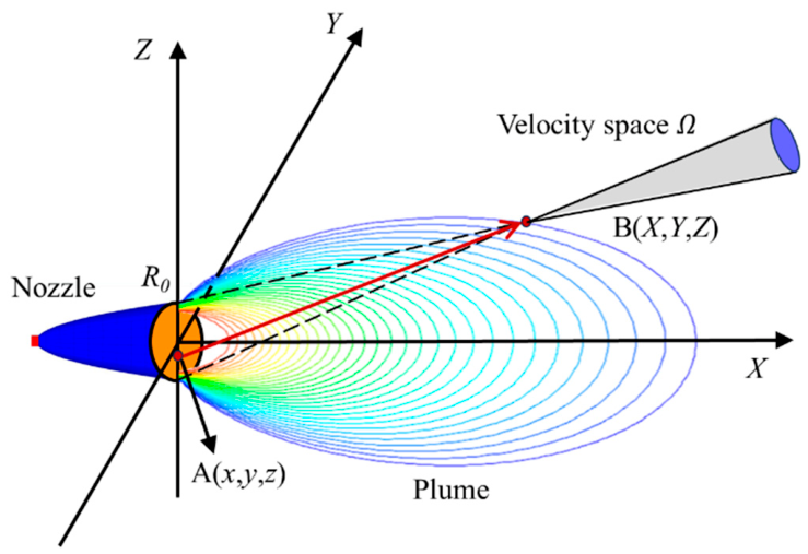
Under these assumptions, a free molecular flow characterized by macroscopic temperature $T_0$, mean velocity $U_0$, and number density $n_0$ at the nozzle exit (radius $R_0$) is ejected into vacuum. The analytical solutions for the flow field parameters were then derived, including the number density, velocity, and temperature at any point downstream of the exit. The equilibrium rarefied-gas velocity distribution follows the Maxwellian form [7]. Only particles whose velocities satisfy geometric constraints at the nozzle exit plane can reach a given downstream point. As depicted in the velocity-space diagram in Figure 1, the exit velocity domain $\mathsf{\Omega }$ is defined by the nozzle geometry [15]:

$$f(u,v,w)=\left\{\begin{array}{c}{\displaystyle \frac{n_0}{\sqrt{{(2R\pi T_0)}^3}}}\exp [{\displaystyle \frac{-(u^2+v^2+w^2)}{2R{T}_0}}] u,v,w\in \mathsf{\Omega };\\ 0\hspace{1em}\hspace{1em}\hspace{1em}\hspace{1em}\hspace{1em}\hspace{1em}\hspace{1em}\hspace{1em}\hspace{1em}\hspace{1em}\hspace{1em}\hspace{1em}\hspace{1em}u,v,w\notin \mathsf{\Omega }\end{array}\right.$$

where $\mathsf{\Omega }$ denotes the integration domain in the velocity phase, $R$ is the gas constant, and $u$, $v$, $w$ represent the instantaneous velocity components.

As shown in Figure 1, for a nozzle with an initial number density $n_0$, velocity $U_0$, temperature $T_0$, and radius $R_0$, the velocity $(u,v,w)$ at a point $A(x,y,z)$ on its cross section can only reach a point $B(X,Y,Z)$ outside the exit cross section if it satisfies the velocity–position relationship given by Equation (1) [16].

$${\displaystyle \frac{X-x}{u+U_0}}={\displaystyle \frac{Y-y}{v}}={\displaystyle \frac{Z-z}{w}}$$

(1)

Based on relevant gas dynamics theories [23], the macroscopic flow field parameters such as the number density, velocity, and temperature can be derived from the velocity distribution function of gas molecules [24]:

$$n_1(X,Y,Z)={\displaystyle \underset{\mathsf{\Omega }}{\int }f(u,v,w)dudvdw}$$

(2)

$$\mathit{U}(X,Y,Z)={\displaystyle \frac{1}{n_1}}{\displaystyle \underset{\mathsf{\Omega }}{\int }\mathit{u}f(u,v,w)dudvdw}$$

(3)

$$T_1(X,Y,Z)={\displaystyle \frac{1}{3R{n}_1}}{\displaystyle \underset{\mathsf{\Omega }}{\int }\left[{(u-U_1)}^2+{(v-V_1)}^2+{(w-W_1)}^2\right]f(u,v,w)dudvdw}$$

(4)

where the subscripts “0” and “1” represent the parameters at the nozzle exit and within the flow field, and $\mathit{U}=(U_1,V_1,W_1)$ represents the macroscopic velocity, $\mathit{u}=(u,v,w)$. Given the axisymmetric nature of the plume about the X-axis, only the flow field distribution in the XOZ plane must be considered. Therefore, in Equation (1), $x$ and $Y$ are set to zero.

Based on Equations (2)–(4), given the velocity distribution $f(u,v,w)$ at a known point $(X,Y,Z)$, the following parameters at $(X,Y,Z)$ can be determined using the velocity distribution function: reference number density-normalized number density, velocity, and translational temperature [25]:

$${\displaystyle \frac{n_1(X,0,Z)}{n_0}}={\displaystyle \frac{\exp (-S_0^2)}{\sqrt{{\pi }^3}{X}^2}}{\displaystyle {\int }_{-\pi /2}^{\pi /2}d\epsilon {\displaystyle {\int }_0^{R_0}rKdr}}$$

(5)

$${\displaystyle \frac{U_1(X,0,Z)}{\sqrt{2R{T}_0}}}={\displaystyle \frac{\exp (-S_0^2)}{\sqrt{{\pi }^3}{X}^2}}{\displaystyle \frac{n_0}{n_1}}{\displaystyle {\int }_{-\pi /2}^{\pi /2}d\epsilon {\displaystyle {\int }_0^{R_0}rMdr}}$$

(6)

$${\displaystyle \frac{W_1(X,0,Z)}{\sqrt{2R{T}_0}}}={\displaystyle \frac{\exp (-S_0^2)}{\sqrt{{\pi }^3}{X}^3}}{\displaystyle \frac{n_0}{n_1}}{\displaystyle {\int }_{-\pi /2}^{\pi /2}d\epsilon {\displaystyle {\int }_0^{R_0}(Z-r\sin \theta )rMdr}}$$

(7)

$${\displaystyle \frac{T_1(X,0,Z)}{T_0}}=-{\displaystyle \frac{U_1^2+W_1^2}{3R{T}_0}}+{\displaystyle \frac{4}{3}}{\displaystyle \frac{\exp (-S_0^2)}{\sqrt{{\pi }^3}{X}^2}}{\displaystyle \frac{n_0}{n_1}}{\displaystyle {\int }_{-\pi /2}^{\pi /2}d\epsilon {\displaystyle {\int }_0^{R_0}rNdr}}$$

(8)

The expressions for variables $K$, $M$, and $N$ are given as follows:

$$K=Q\left\{Q{S}_0\right.+\left[{\displaystyle \frac{1}{2}}+Q{S}_0^2\right]\sqrt{\pi Q}[1+\mathrm{erf}(S_0\sqrt{Q})]\left.\exp (S_0^{2}Q)\right\}$$

(9)

$$M=Q^2\{Q{S}_0^2+1+S_0[{\displaystyle \frac{3}{2}}+Q{S}_0^2]\sqrt{\pi Q}[1+erf(\sqrt{Q}{S}_0)]\exp (S_0^{2}Q)\}$$

(10)

$$N={\displaystyle \frac{S_0{Q}^2}{2}}[{\displaystyle \frac{5}{2}}+Q{S}_0^2]+{\displaystyle \frac{\sqrt{Q^3\pi }}{2}}[{\displaystyle \frac{3}{4}}+3Q{S}_0^2+Q^2{S}_0^4]{[1+\mathrm{erf}(\mathrm{S}}_0\sqrt{Q}{\left)\right]\mathrm{e}}^{{\mathrm{S}}_0^2\mathrm{Q}}$$

(11)

where $S_0=U_0/\sqrt{2R{T}_0}$; the $Q$ variable expression is given as follows:

$$Q={\cos }^2\psi {[{\displaystyle \sum _{n=0}^{\infty }}{P}_n(\sin \psi \sin \epsilon ){({\displaystyle \frac{r}{\sqrt{X^2+Z^2}}})}^n]}^2$$

(12)

where $P_n(\sin \psi \sin \epsilon )$ is the Legendre Polynomial; $\psi =\arctan (Z/X)$.

2.3. Multi-Component Vacuum Plume Model

Previous engineering models neglected multicomponent plume characteristics [6,15,16,17,18,19]. In practice, unsteady fuel–oxidizer reactions yield multicomponent combustion gases whose composition varies with chamber temperature, pressure, and mixture ratio.

To compute mixed-gas number density, temperature, and velocity distributions, we first determine the mixture gas constant as the molar-fraction-weighted average of component gas constants:

$$R={\displaystyle \sum _{s=1}^N{Y}_{0s}{R}_s}$$

(13)

where $Y_{0s}$ denotes the molar fraction of component $s$ at the exit and $R_s$ represents its gas constant.

The source strength $S_{0s}$ of each component, needed for molar fractions and pressure distribution, is expressed as follows:

$$S_{0s}={\displaystyle \frac{U_0}{\sqrt{2R_s{T}_0}}}$$

(14)

where $S_{0s}$ represents the source strength of the component $s$. By incorporating these values, along with other initial parameters, into the plume model, the number density $n_s$ distribution for each component $s$ can be calculated. The molar fraction distribution of each component is then determined as

$$Y_s={\displaystyle \frac{n_s}{{\displaystyle \sum _{s=1}^N{n}_s}}}$$

(15)

where $Y_s$ denotes the molar fraction of the component $s$. The normalized molar fraction ${\eta }_s$ for each component is defined as

$${\eta }_s={\displaystyle \frac{Y_s}{Y_{s,\mathrm{e}}}}$$

(16)

2.4. Interaction Model Between Incoming Flow and Plume

When the combustion gas at the nozzle exit expands ideally and entropically from its initial stagnation state to an absolute vacuum, the theoretical maximum exhaust velocity is determined by gas thermodynamics [26]:

$$U_{\max }=\sqrt{2h_{\mathrm{e}}}=\sqrt{2{\displaystyle \frac{{\gamma }_{\mathrm{e}}{R}_{\mathrm{e}}{T}_{\mathrm{e}}}{{\gamma }_{\mathrm{e}}-1}}}$$

(17)

where $h_{\mathrm{e}}$ denotes the total enthalpy per unit mass of the combustion gas at the nozzle exit, ${\gamma }_{\mathrm{e}}$ indicates the specific heat ratio of the gas at the nozzle exit, $R_{\mathrm{e}}$ represents the gas constant of the combustion gas at the nozzle exit, and $T_{\mathrm{e}}$ denotes the stagnation temperature at the nozzle exit.

The total collision number for a molecule traveling from the nozzle exit to the target point is:

$$c=n_{\mathrm{c}}{\sigma }_{\mathrm{ref}}{k}_{p}L$$

(18)

where $L$ denotes the distance from the nozzle point source to the target point, $n_{\mathrm{c}}$ represents the number density of the incoming flow, ${\sigma }_{\mathrm{ref}}$ denotes the particle collision cross-sectional area, and $k_{\mathrm{p}}$ indicates the probability of a fully elastic collision. Based on the phenomenon that the drag force in a free molecular flow over a sphere generally decreases with increasing relative molecular speed ratio $s_{\mathrm{r}}=U_{\max }/\sqrt{2R_{\infty }{T}_{\infty }}$, the probability $k_{\mathrm{p}}=1/s_{\mathrm{r}}$ of a fully elastic collision can be expressed as a function of this ratio.

The collision process between a plume particle and an incoming flow particle can be specifically described as follows: a plume particle micro-group with volume $\mathsf{\Delta }V$, mass ${\displaystyle \sum n_s{m}_s\mathsf{\Delta }V}$, and velocity $U_{\max }$ undergoes a non-central fully elastic collision with an incoming flow particle of volume $\mathsf{\Delta }V$, mass $c{n}_c{m}_c\mathsf{\Delta }V$, and velocity $U_{\infty }$. The velocity components $U^{\prime }$ and $W^{\prime }$ are determined as follows [26]:

$$U^{\prime }={\displaystyle \frac{U_{\max }\cos \theta ({\displaystyle \sum _s{n}_s{m}_s}-c{n}_c{m}_c)+2c{n}_c{m}_c{U}_{\infty }}{{\displaystyle \sum _s{n}_s{m}_s}+c{n}_c{m}_c}}$$

(19)

$$W^{\prime }={\displaystyle \frac{U_{\max }\sin \theta ({\displaystyle \sum _s{n}_s{m}_s}-c{n}_c{m}_c)}{{\displaystyle \sum _s{n}_s{m}_s}+c{n}_c{m}_c}}$$

(20)

These molecules then travel to a new location $(x^{\prime },o,z^{\prime })$ with the positional correspondence between $(x,o,z)$ and $(x^{\prime },o,z^{\prime })$ provided as

$${\displaystyle \frac{x^{\prime }}{x}}={\displaystyle \frac{U_{\max }\cos \theta \mathsf{\Delta }t+U^{\prime }\mathsf{\Delta }t}{2U_{\max }\cos \theta \mathsf{\Delta }t}}={\displaystyle \frac{U_{\max }\cos \theta +U^{\prime }}{2U_{\max }\cos \theta }}$$

(21)

$${\displaystyle \frac{z^{\prime }}{z}}={\displaystyle \frac{U_{\max }\sin \theta \mathsf{\Delta }t+W^{\prime }\mathsf{\Delta }t}{2U_{\max }\sin \theta \mathsf{\Delta }t}}={\displaystyle \frac{U_{\max }\sin \theta +W^{\prime }}{2U_{\max }\sin \theta }}$$

(22)

2.5. Calculation Mode of Plume Parameters

Macroscopic flow parameters of the gas mixture are calculated via the density-weighted averaging method [27]. Total number density:

$$n={\displaystyle \sum _{s^{\prime }}{n}_{s^{\prime }}}={\displaystyle \sum _s{n}_s}+{\displaystyle \sum _c{n}_c}$$

(23)

Mass density:

$$\overline{\rho }=\overline{m}n={\displaystyle \sum _{s^{\prime }}{n}_{s^{\prime }}{m}_{s^{\prime }}}={\displaystyle \sum _{s^{\prime }}{\rho }_{s^{\prime }}}$$

(24)

Average velocity components:

$$\overline{U}={\displaystyle \frac{{\displaystyle \sum _{s^{\prime }}{\rho }_{s^{\prime }}{U}_{s^{\prime }}}}{{\displaystyle \sum _{s^{\prime }}{\rho }_{s^{\prime }}}}}={\displaystyle \frac{{\displaystyle \sum _s{m}_s{n}_s{U}_s}+{\displaystyle \sum _c{m}_c{n}_c{U}_c}}{{\displaystyle \sum _{s^{\prime }}{\rho }_{s^{\prime }}}}}$$

(25)

$$\overline{W}={\displaystyle \frac{{\displaystyle \sum _{s^{\prime }}{\rho }_{s^{\prime }}{W}_{s^{\prime }}}}{{\displaystyle \sum _{s^{\prime }}{\rho }_{s^{\prime }}}}}={\displaystyle \frac{{\displaystyle \sum _s{m}_s{n}_s{W}_s}}{{\displaystyle \sum _s{\rho }_s}}}$$

(26)

Mixture gas constant:

$$\overline{R}={\displaystyle \sum _{s^{\prime }}\frac{n_{s^{\prime }}}{n}{R}_{s^{\prime }}}$$

(27)

The expression for calculating the statistical temperature $T$ is as follows [26]:

$$T={\displaystyle \frac{1}{3+\zeta }}(3{\displaystyle \frac{Q_{tr}+1.5({\displaystyle \sum _s{m}_s{R}_s{n}_s{T}_s}+{\displaystyle \sum _c{m}_c{R}_c{n}_c{T}_c})}{1.5({\displaystyle \sum _s{m}_s{R}_s{n}_s+{\displaystyle \sum _c{m}_c{R}_c{n}_c}})}}+\zeta {\displaystyle \frac{{\displaystyle \sum _s{m}_s(c-1.5R_s)n_s{T}_s}+{\displaystyle \sum _c{m}_c{n}_c{T}_c}}{{\displaystyle \sum _s{m}_s(c-1.5R_s)n_s}+{\displaystyle \sum _c{m}_c{n}_c}}})$$

(28)

where $Q_{tr}$ and $\zeta$ denoting variable expression are given as follows:

$$Q_{tr}={\displaystyle \frac{1}{2}}{\displaystyle \sum _s{n}_s{m}_s(U_s^2+W_s^2)}+{\displaystyle \frac{1}{2}}{\displaystyle \sum _c{n}_c{m}_c{U}_c}-\overline{\rho }({\overline{U}}^2+{\overline{W}}^2)$$

(29)

$$\zeta ={\displaystyle \sum _{s^{\prime }}2{\rho }_{s^{\prime }}(c-1.5R_{s^{\prime }})}$$

(30)

The aforementioned density-weighted averaging is solely employed to derive macroscopic bulk flow properties; in Section 3, however, species-specific mole fractions and number densities are retained and utilized for the calculation of species-resolved spectral radiation parameters.

2.6. Infrared Radiative Calculation Model

To simplify the computational process, this study neglects non-equilibrium radiation effects and adopts the same infrared radiation calculation methodology used for continuum flow plume simulations [28]. However, this simplification is physically justified by the specific operating conditions of our study: the Maxwellian velocity distribution assumption is adopted, which is valid for the high-vacuum free molecular flow regime (altitudes above 120 km) considered in this work. Under these conditions, rotational–translational equilibrium is already achieved at the nozzle exit plane, and vibrational non-equilibrium effects have a negligible impact on infrared radiation due to the extremely low collision frequency. For transition flow regimes at lower altitudes, non-equilibrium effects would need to be explicitly considered. Accordingly, we employed a statistical narrowband (SNB) model to compute the radiative properties of the plume. The common SNB model variations include the standard, Goody, and Malkmus models [29]. The Malkmus SNB model offers the highest accuracy and was thus selected for this study. In this model, the spectral line intensity is assumed to follow an exponentially tailed inverse distribution. Considering the total pressure $P$, species mole fraction $x$, and path length $l_m$, the average transmissivity within a narrowband can be calculated as [30]

$$\overline{{\tau }_{\eta }}(x)=\exp \left\{-2{\displaystyle \frac{\overline{\gamma }}{\overline{d}}}\left[{\left(1+x\cdot P\cdot l_m\cdot \overline{\kappa }\cdot {\displaystyle \frac{\overline{d}}{\overline{\gamma }}}\right)}^{{\displaystyle \frac{1}{2}}}-1\right]\right\}$$

(31)

where $\overline{\gamma }$ denotes the mean line half-width; $\overline{d}$ indicates the mean line spacing; and $\overline{\kappa }$ represents the average absorption coefficient of the spectral band. For engine exhaust gases composed of multiple species such as H₂O, CO₂, and CO, the mean line half-width for each gas component can be calculated using the empirical equation [31].

The average absorption coefficient $\overline{\kappa }$ within the spectral band can be obtained from the line intensities $S_i$ of $N$ spectral lines over the averaging interval $\mathsf{\Delta }\eta$ as follows:

$$\overline{\kappa }={\displaystyle \frac{1}{\mathsf{\Delta }\eta }}{\displaystyle \sum _{i=1}^N}{S}_i$$

(32)

Upon determining the mean line half-width and average absorption coefficient within the spectral band, the mean line spacing $\overline{d}$ can be expressed as

$$\overline{d}={\displaystyle \frac{\overline{\kappa }\cdot \overline{\gamma }}{{\left(\frac{1}{\mathsf{\Delta }\eta }{\displaystyle \sum _{i=1}^N}\sqrt{S_i}\right)}^2}}$$

(33)

The radiative properties for major plume species were obtained from NASA-SP-3080 [32] and compiled into a narrowband database covering 100–3000 K. The required averages of the transmissivity data were generated through wavenumber–temperature interpolation with pressure corrections.

3. Computational Method

3.1. Radiative Transfer Calculation Model

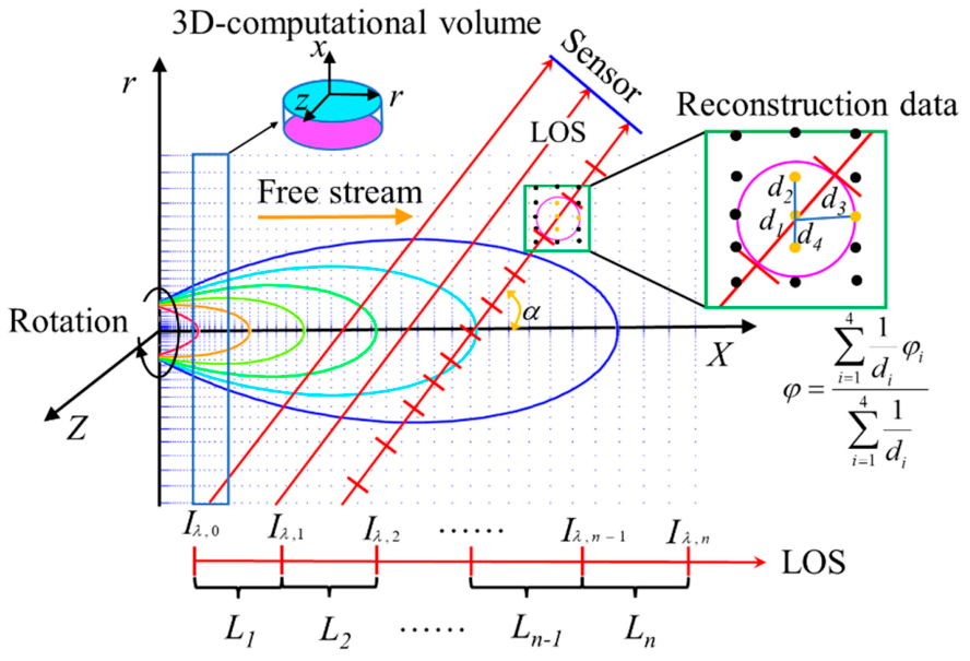
This study did not consider the phase variations in the plume components; thus, the flow field did not contain scattering media. Neglecting the phase changes, we applied the line-of-sight (LOS) method (Figure 2) to compute radiative transfer. The LOS approach simplifies the representation of radiation transfer by translating the 3D inhomogeneous media into a 1D multilayer problem, which enables efficient computation. Figure 2 presents the overall computational procedure of the LOS method, with each step detailed as follows:

(a)

Divide the line-of-sight path into uniform computational layers;

(b)

Reconstruct the flow properties (temperature, pressure, and species mole fractions) of each layer via four-node inverse-distance weighting interpolation;

(c)

Calculate the spectral absorption coefficient based on the layer-averaged properties;

(d)

Solve the radiative transfer equation sequentially along each layer and accumulate to obtain the final exit intensity.

Rotating the 2D planar flow field about its axis produced a 3D cylindrical domain. The parallel rays traversed this domain, which was segmented into homogeneous layers. Four-node inverse-distance weighting (Figure 2) reconstructed flow properties in each layer [33].

This can be expressed as [34]

$${\displaystyle \frac{{\mathrm{dI}}_{\lambda }(l,\overrightarrow{l})}{\mathrm{d}l}}={\kappa }_{\lambda }(l)[I_{b\lambda }(l)-I_{\lambda }(l,\overrightarrow{l})]$$

(34)

where $l$ denotes the radiation transfer path; $\overrightarrow{l}$ indicates the path length vector; $\lambda$ represents the wavelength; $I_{\lambda }$ denotes the spectral radiation intensity; $I_{b\lambda }$ indicates the blackbody radiation intensity; and ${\kappa }_{\lambda }$ represents the spectral absorption coefficient. As ${\tau }_{\lambda }(l)={\kappa }_{\lambda }(l)\mathrm{d}l$, Equation (34) can be rewritten in a differential form using the spectral optical thickness:

$${\displaystyle \frac{d{I}_{\lambda }({\tau }_{\lambda },\overrightarrow{l})}{d{\tau }_{\lambda }}}=I_{b\lambda }(s)-I_{\lambda }({\tau }_{\lambda },\overrightarrow{l})$$

(35)

The spectral radiation intensity of the $i$-th grid cell along the $\overrightarrow{l}$ direction can be expressed as follows:

$$I_{\lambda ,i}(\overrightarrow{l})=I_{\lambda ,i-1}(\overrightarrow{l})\exp (-{\tau }_{\lambda ,i})+I_{b\lambda ,i}[1-\exp (-{\tau }_{\lambda ,i})]$$

(36)

Integrating Equation (36) in the direction opposite to the detection ray yields the boundary-emitted spectral radiation intensity along the $\overrightarrow{l}$ direction:

$$I_{\lambda }(\mathrm{l})=I_{\mathrm{b}\lambda ,n}[1-{\exp }^{-{\tau }_{\lambda .n}}]+{\displaystyle \sum _{i=1}^{n-1}}\left[\exp \left(-{\displaystyle \sum _{j=i+1}^n}{\tau }_{\lambda .j}\right)-\exp \left(-{\displaystyle \sum _{j=i}^n}{\tau }_{\lambda .j}\right)\right]I_{\mathrm{b}\lambda ,i}$$

(37)

where $n$ denotes the total number of layers penetrated by the ray, ${\tau }_{\lambda j}$ represents the spectral optical thickness of the $j$-th grid cell, and $I_{b\lambda j}$ denotes the blackbody spectral radiation intensity at the temperature $T_i$ of the $i$-th grid cell.

3.2. Computational Process

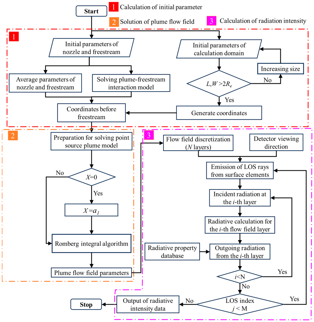
Based on the physical characteristics of vacuum plumes and the requirements for efficient engineering prediction, this study adopts the point-source vacuum plume model (PSVPM), the Malkmus statistical narrowband model, and the line-of-sight (LOS) method. The PSVPM is selected for its advantage in computational efficiency and is extended to accommodate multicomponent gas calculations and plume–freestream non-central elastic collision interactions. The Malkmus model is employed for high-fidelity spectral radiation calculations, while the LOS method is optimized for axisymmetric flow fields. The coupling framework utilizes density-weighted averaging and Romberg integration to achieve a balance between prediction accuracy and computational cost. As illustrated in Figure 3, the engineering model comprises three phases: computing initial flow field parameters, solving the plume flow field, and calculating radiative intensity.

The computational workflow of the proposed PSVM-IR-LOS coupled framework consists of three core stages. The initial parameters include nozzle and freestream conditions as well as computational domain specifications. The domain is discretized, and plume coordinates are established prior to freestream interaction. When domain dimensions are smaller than the nozzle diameter, the solution is truncated, requiring domain resizing. In the second stage, the Romberg integration algorithm is employed to solve the point-source vacuum plume model. To ensure numerical stability, singular points on the Z-axis are replaced with adjacent regular points, yielding plume flow parameters including number density, velocity, temperature, and species mole fractions. In the third stage, radiative properties are determined from the flow field with supplementary NASA-3080 database data, and the line-of-sight (LOS) method is applied to compute radiative transfer. The plume is discretized into uniform computational layers, and radiation intensity is calculated iteratively along each detector ray to obtain spectral radiation intensity over specified wavenumber ranges.

4. Results and Discussion

4.1. Validation of Flow Field Parameters for Vacuum Plume Model

4.1.1. Verification of Ar Plume

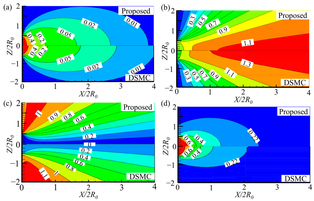
The reliability of the proposed vacuum plume engineering model was validated against the DSMC results for plume flows [19]. The DSMC method simulates real molecules using computational particles accounting for molecular collisions and offering high accuracy, which has been widely adopted for high-altitude plume simulations. The reference study specifies a nozzle radius of 0.5 m, pure argon (Ar) as the medium, a nozzle exit static temperature $T_0$ of 300 K, and a velocity ratio $S_0$ of 0.5. These simulation parameters were used as inputs to compute the vacuum plume. The selected conditions included zero freestream velocity ($U_{\infty }=0\mathrm{m}/\mathrm{s}$) and an altitude of $H=200\mathrm{km}$ corresponding to the ambient number density of $7.2\times {10}^{15}{\mathrm{m}}^{-3}$. Figure 4 presents the normalized plume parameter distributions. Subplots (a), (b), (c), and (d) display the normalized number density, velocity $U$, velocity $W$, and temperature distributions, respectively. Upper halves present model results; lower halves depict DSMC data.

The computed plume flow field parameters were consistent with the DSMC reference data and exhibited consistent distribution patterns. The calculated number density and velocity distributions closely aligned with the reference values. However, as shown in Figure 4, noticeable deviations were observed in the axial and radial velocities within the far-field expansion zone. Since macroscopic velocity is not directly involved in radiation calculations and exerts only a minor influence on temperature via statistical averaging, these velocity deviations have a negligible impact on subsequent infrared signature prediction. As depicted in Figure 4a, the plume number density attains its maximum at the nozzle exit and decays rapidly in an elliptical downstream pattern. The number density peaks at the exit and decays elliptically downstream, with a 7% deviation from DSMC. Core-region axial velocity increases at a distance from the exit, and velocity contours straighten downstream. According to Equation (8), marginally lower computed velocities resulted in correspondingly higher temperature values, particularly at positions farther from the nozzle, where the maximum deviation from the DSMC results was approximately 18%. These comparisons confirm the reliability of the engineering model.

4.1.2. Verification of Multi-Species MBB Engine Plume

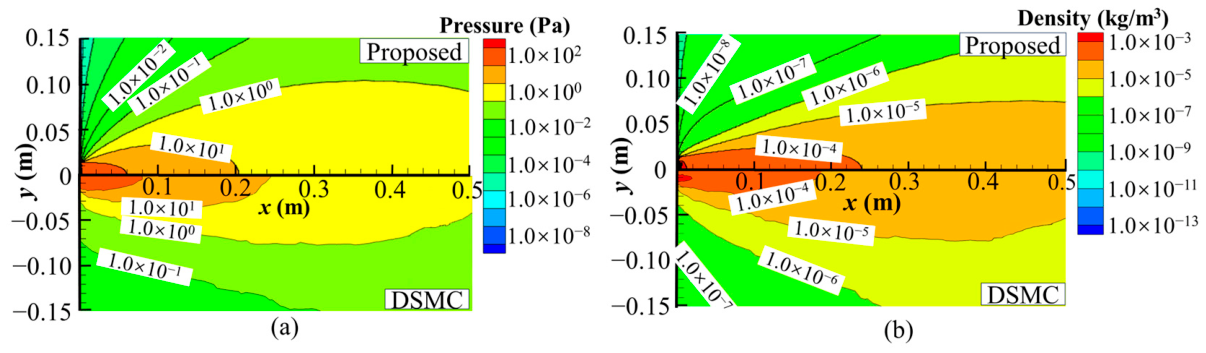
The MBB 10 N engine is a bipropellant, low-thrust satellite thruster with a 35 mm nozzle exit, U₀ = 3117 m/s, and T₀ = 682 K. The exhaust gas mass fractions are listed in

Table 1. Main components and mole fractions at the nozzle outlet plane.

Major species	H2O	N2	H2	CO	CO2	H	OH	NO	Σ(O2, O)
Mole fraction	0.324	0.304	0.157	0.130	0.037	0.024	0.017	2.6 × 10−3	3.1 × 10−3

. Chae et al. [35] used a fully unstructured 3D DSMC code to simulate MBB plume distributions for model validation. Figure 5a,b compare pressure and density distributions: upper halves depict the present model; lower halves display DSMC results. The engineering model predicts plume pressure that is ∼15% lower along the axis and density that is ∼10% higher than DSMC. These outcomes indicate that the multicomponent plume predictions of the engineering model align well with high-fidelity DSMC simulations, validating its applicability for rapid plume prediction.

The pressure and density distributions are comparatively presented in Figure 5a and Figure 5b, respectively, with the upper halves displaying the results from the present model and the lower halves displaying the reference data. The engineering model results showed slightly lower values than the DSMC-calculated flow field distributions. Specifically, the plume pressure computed using the engineering algorithm was ~15% lower along the axial direction, whereas the density was ~10% higher than the DSMC results. These comparisons demonstrate that the plume flow field predictions from the engineering model generally align with the high-fidelity DSMC simulations, thereby validating the reliability of the vacuum plume engineering model for multicomponent plume predictions.

4.1.3. Validation of the Infrared Radiation Computation Model

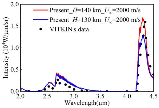
Publicly reported infrared spectral data for vacuum and high-altitude plumes remain scarce. Vitkin et al. [36] developed a computational model based on the Navier–Stokes equations, augmented with chemical kinetics and vibrational relaxation terms, to characterize plume flow and radiation in inhomogeneous, non-equilibrium media. This model was applied to compute the infrared, visible, and ultraviolet spectra of a liquid–rocket engine vacuum plume, thus providing a suitable validation case for the present rapid engineering model. The nozzle parameters of the liquid engine selected by Vitkin et al. are listed in

Table 2. Flow field parameters and mole fraction of species on the exit plane.

De, m	Te, K	Ue, m/s	Pe, atm	Molar Fraction of Species
				H2	H2O	CO	CO2	N2
1	2000	2500	0.3	0.05	0.4	0.05	0.15	0.35

and include a nozzle radius of 0.5 m and an exhaust composition comprising five species. Their spectral calculations yielded radiation data over the 2.0–4.5 μm wavelength range.

The flow field computation employed a computational domain with axial and radial dimensions of 50 m and 30 m, respectively. As the reference study did not specify altitude or freestream velocity, two simulation conditions were selected: altitudes of 130 km and 140 km, both with a freestream velocity of 2000 m/s. The radiation spectrum in the 2.0–4.5 μm band, calculated at a spectral resolution of 5 cm⁻¹, agrees well with the reference data, as depicted in Figure 6. The close alignment of spectral peak and valley positions confirms the reliability of the present computational model.

4.2. Analysis of Vacuum Plume Diffusion Characteristics

A detailed multicomponent plume flow field analysis is conducted under high-vacuum conditions using the Titan Stage 2 engine [37] as a case study, with the exhaust plume treated as free molecular flow. The nozzle exit diameter is 26.03 inches, with an initial temperature of 1367 K, an initial pressure of 0.1388 atm, and an initial velocity of 3061 m/s.

Table 3. Flow field mole fraction of species on the exit plane.

Major species	CO2	H2O	H2	N2	H	CO	NO	OH	Σ(O2, O, N)
Mole fraction	0.1051	0.4652	0.0185	0.3563	0.0089	0.0141	0.0141	0.0021	0.0167

lists the species and corresponding parameters of the exhaust gas composition.

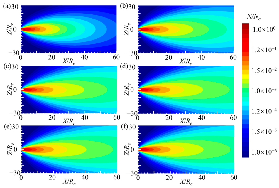
This section presents the plume flow field calculations for six altitudes ranging from $H$ = 120 km to $H$ = 500 km under an oncoming flow velocity of 2500 m/s. Figure 7 depicts the contours of the normalized number density distributions at the six selected altitudes. All distributions exhibit characteristic “feather-like” structures. With increasing altitude, the plume demonstrated progressively greater expansion, especially along the axial direction, as illustrated in Figure 7a–d. At higher altitudes, depicted in Figure 7d–f, the number density distributions underwent minimal further changes, indicating that plume expansion had approached a spatial limit. Considering oncoming flow effects, the environmental molecular number density decreased with increasing altitude. Consequently, the interaction between the oncoming flow and the plume weakened, enabling greater radial expansion of the plume. These results clarify the combined influence of altitude and oncoming flow on plume morphology. Under near-vacuum conditions, where oncoming flow effects become negligible, plume expansion gradually ceases and the number density distribution stabilizes. This morphological evolution is driven by changes in the plume–freestream interaction layer, a thin shear region formed by binary molecular collisions at the plume–atmosphere interface. At lower altitudes (120–200 km), high freestream density leads to frequent collisions, creating a thin but high-temperature interaction layer that compresses the plume radially. As altitude increases above 200 km, the collision frequency drops exponentially, the interaction layer thickens and weakens, and the plume expands freely to form the characteristic “feather-like” structure. Above 300 km, the interaction becomes negligible, and plume expansion stabilizes at the free molecular limit.

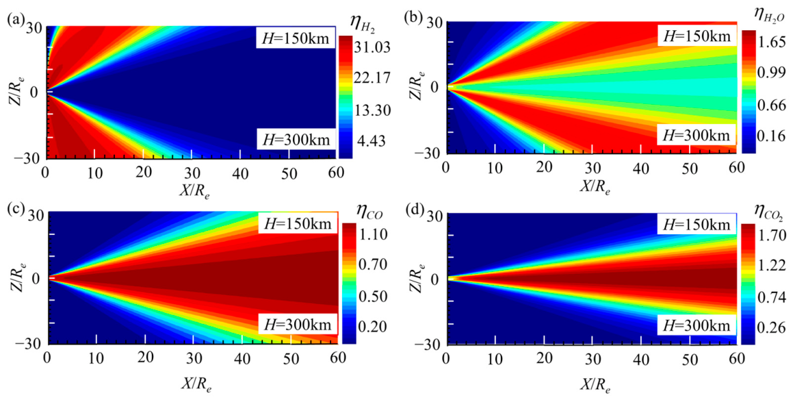
To examine the altitude effect on plume species distribution, Figure 8 presents contours of normalized molar fractions for representative species at $H$ = 150 km (upper half) and $H$ = 300 km (lower half) under a freestream velocity of 2500 m/s. Figure 8a–d depict the axial and radial distributions of H₂, H₂O, CO, and CO₂, respectively. The heaviest species, CO₂, concentrates near the plume centerline due to high inertia, the lightest H₂ disperses near the nozzle exit with significant radial spread, and intermediate-mass H₂O reaches its peak molar fraction at a characteristic off-axis angle. Altitude exerts limited influence on species molar fraction distributions: only H₂ shows marginally greater radial expansion near the nozzle exit at higher altitude, while H₂O, CO and CO₂ distributions remain nearly unchanged, consistent with reported DSMC results [38] and experimental measurements [39]. This distribution pattern arises from species-dependent radial diffusion tendencies: heavier molecules retain initial axial momentum with minimal radial dispersion, while lighter species undergo extensive radial diffusion, and intermediate-mass species exhibit transitional behavior.

4.3. Thermal Distribution Characteristics of Vacuum Plume

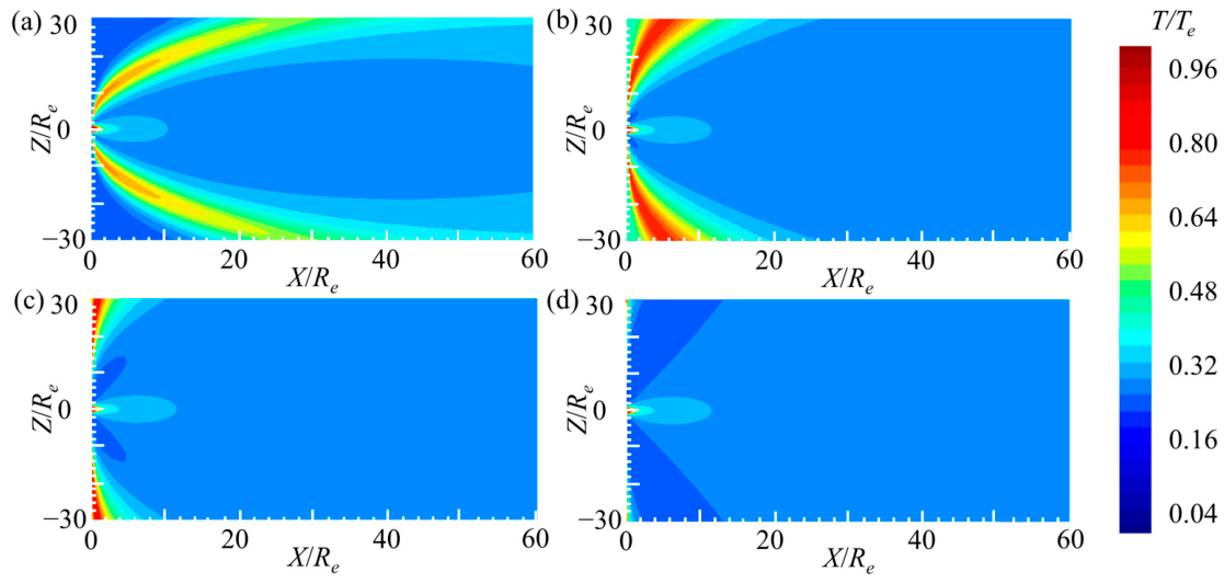
Building on the preceding section’s systematic analysis of multicomponent exhaust plume diffusion characteristics under high-vacuum conditions, this section focuses on the evolutionary characteristics of the plume temperature field and its variation patterns under different flight conditions. Figure 9 shows the contours of normalized temperature distribution for the plume at altitudes of 120 km to 500 km, revealing distinct stagewise evolution of the plume temperature field with increasing altitude. In the 120–200 km low-altitude range, a pronounced localized high-temperature region with strong axial and radial temperature gradients appears near the nozzle exit. As altitude rises to 200–300 km, the high-temperature zone contracts progressively, the overall temperature gradient decreases significantly, and the temperature distribution becomes more uniform. This evolutionary behavior is dominated by the combined effects of ambient atmospheric rarefaction and freestream–plume interaction. Increasing altitude continuously reduces the ambient molecular number density, weakening the momentum and energy exchange between the freestream and the plume. At low altitudes, strong freestream–plume interaction induces intense kinetic energy transfer in the low-velocity region near the nozzle exit, forming the localized high-temperature zone. At higher altitudes, the rarefied atmosphere substantially suppresses freestream–plume interaction, the free expansion of the plume gradually dominates, and the inter-molecular collision probability decreases significantly. Eventually, the high-temperature region near the nozzle exit vanishes, and the plume temperature distribution stabilizes.

4.4. Evaluation of Calculation Efficiency

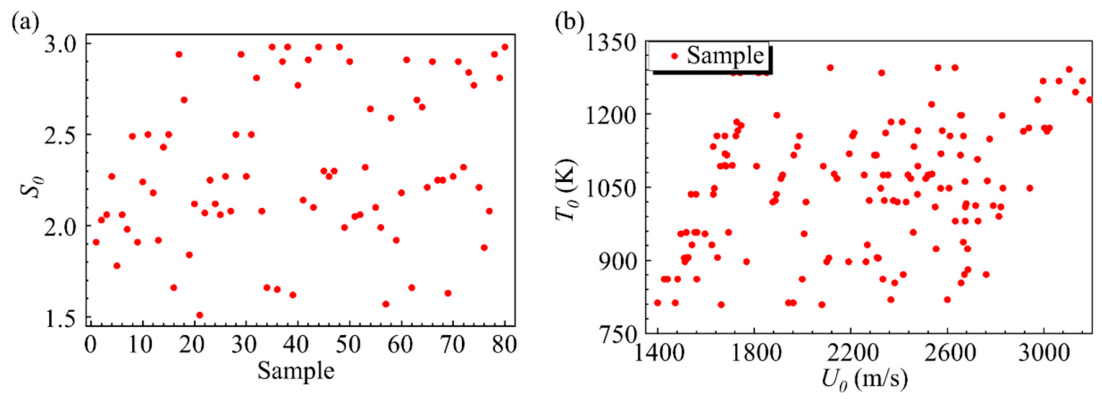
Using the Titan Stage 2 engine as a case study and accounting for variations in the velocity ratio $S_0$ across different rocket engine types, we selected 80 distinct nozzle-exit conditions, each with a specific $S_0$ value, as depicted in Figure 10a. Figure 10b presents a scatter plot of the initial nozzle-exit velocities and corresponding initial temperature values for each individual sample.

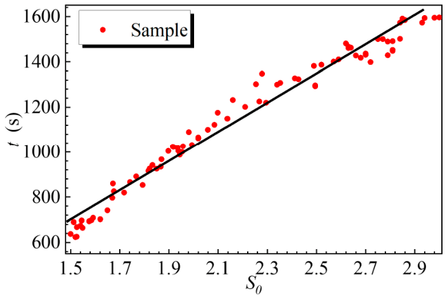
When conventional DSMC methods are employed for plume flow field simulations, the average computation time per case is typically on the order of 10⁵ s [12]. Figure 11 portrays that the engineering algorithm requires between 600 and 1400 s, which lies within the 10³ s range. This represents a substantial reduction compared with traditional DSMC methods. Furthermore, a clear positive correlation exists between computation time and the parameter $S_0$. In the engineering computational approach, the Romberg integration algorithm is utilized to evaluate model integrals. As $S_0$ increases, the exponential term “$\exp (A{S}_0^2)$” in the integrand, where A depends on the computational domain coordinates, grows rapidly. This increase generates a steeper peak near the right endpoint $b$ of the integration interval $(a,b)$. Consequently, the Romberg integration algorithm demands finer domain discretization and additional iterations to meet accuracy requirements, thereby prolonging its convergence time.

4.5. Analysis of Infrared Radiation Characteristics

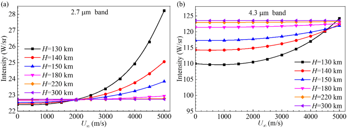
This section presents calculations of plume radiation for freestream velocities from $U_{\infty }$ = 0 to 5000 m/s and altitudes from $H$ = 130 to 300 km. Figure 12 depicts the variation in integrated radiation intensity with freestream velocity at different altitudes for the 2.7 μm and 4.3 μm bands. The results demonstrate that increasing freestream velocity enhances integrated radiation intensity at all altitudes and in both bands, although this effect diminishes at higher altitudes. At $H$ = 130 km, when the freestream velocity is increased from 0 to 5000 m/s, the plume radiation intensity increases by 25.9% at the 2.7 μm band and by 12.9% at the 4.3 μm band. At $H$ = 150 km, the same velocity increase from 0 to 5000 m/s yields smaller enhancements: 5.7% at 2.7 μm and 3.9% at 4.3 μm.

This behavior is attributed to intensified momentum exchange between the freestream and plume at higher velocities, which elevates translational kinetic energy in the core interaction region and thus increases plume temperature. The 2.7 μm band shows higher sensitivity to freestream velocity because H₂O concentrates adjacent to the core momentum exchange region. With increasing altitude, atmospheric rarefaction weakens freestream–plume interaction, gradually reducing the influence of freestream velocity on radiation intensity.

A quantitative contribution analysis shows that the interaction layer accounts for 18.7% of the total radiance at 130 km, but this contribution drops to 6.2% at 150 km and less than 2% above 200 km. The higher sensitivity of the 2.7 μm band to freestream velocity arises because lighter H₂O molecules concentrate in the interaction layer, while heavier CO₂ molecules (dominant in the 4.3 μm band) remain primarily in the plume core. The net increase in radiance at high altitudes is due to the expanded radiative volume, which outweighs the slight reduction in gas temperature.

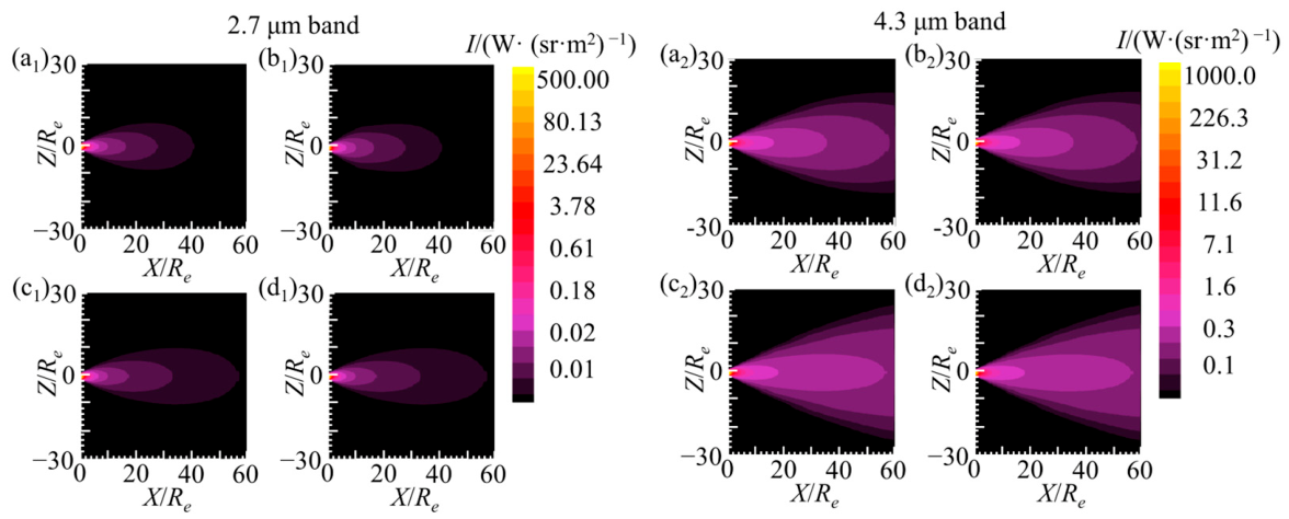
Synthetic IR images of the two bands at $H$ = 150 km and 220 km under freestream velocities of 3000 m/s and 5000 m/s are presented in Figure 13. Both bands exhibit characteristic feather-like radiance distributions, with the 4.3 μm band displaying substantially higher overall radiance than the 2.7 μm band. Overall radiance intensifies with increasing altitude due to greater plume expansion enabled by reduced freestream–plume interaction, while the influence of freestream velocity on radiance distribution becomes less pronounced. The significantly higher radiance in the 4.3 μm band confirms that CO₂ is the dominant contributor to total plume radiation for the Titan Stage 2 engine exhaust.

5. Conclusions

This study presents an engineering methodology for rapid prediction of infrared radiation characteristics from engine vacuum plumes. By integrating multiple physical models, this approach enables end-to-end computation from plume flow field generation to infrared radiative transfer. For the Titan Stage 2 engine test case, the main conclusions are as follows:

• The methodology employs a point-source plume model for circular nozzles and incorporates multicomponent exhaust gases, plume–freestream interactions, and density-weighted averaging to calculate macroscopic flow parameters. The model predicted plume distributions across altitudes and freestream velocities with validation errors within 20%, thus meeting engineering accuracy requirements.
• When combined with infrared radiative transfer modeling, the plume flow field framework constitutes a comprehensive computational approach for vacuum plume infrared characteristics. This method reliably calculated spectral radiance distributions and integrated radiation intensity, producing results consistent with established physical trends.
• The engineering approach rendered computational speeds two to three orders of magnitude faster than conventional DSMC methods, significantly improving efficiency. Computation time exhibited a strong positive correlation with the parameter $S_0$.
• As altitude increases, the influence of freestream on plume diffusion and translational kinetic energy diminishes and nearly ceases under near-vacuum conditions, whereas the effect of freestream velocity on radiation intensity decreases with altitude. Greater plume expansion at higher altitudes intensifies overall radiation.

References

1. U.S. Committee on Extension to the Standard Atmosphere. U.S. Standard Atmosphere; National Oceanic and Atmospheric Administration: Washington, DC, USA, 1976.
2. Paiva, C.; Slusher, H. Space-Based Missile Exhaust Plume Sensing: Strategies for DTCI of Liquid and Solid IRBM Systems. In Space; American Institute of Aeronautics and Astronautics: Long Beach, CA, USA, 2005; p. 6820. [Google Scholar] [CrossRef]
3. Cai, G.; Liu, L.; He, B.; Ling, G.; Weng, H.; Wang, W. A review of research on the vacuum plume. Aerospace 2022, 9, 706. [Google Scholar] [CrossRef]
4. Chung, C.-H.; Kim, S.C.; Stubbs, R.M. Low-density nozzle flow by the direct simulation Monte Carlo and continuum methods. J. Propuls. Power 1995, 11, 64–70. [Google Scholar] [CrossRef]
5. He, B.; Zhang, J.; Cai, G. Research on vacuum plume and its effects. Chin. J. Aeronaut. 2013, 26, 27–36. [Google Scholar] [CrossRef]
6. Cai, C.; Boyd, I.D. Collisionless gas expanding into vacuum. J. Spacecr. Rocket. 2007, 44, 1326–1330. [Google Scholar] [CrossRef]
7. Bird, G.A. Molecular Gas Dynamics and the Direct Simulation of Gas Flows; Oxford University Press: Oxford, UK, 1994. [Google Scholar]
8. Bird, G.A. Molecular gas dynamics. NASA STI/Recon Tech. Rep. A 1976, 76, 40225. [Google Scholar]
9. Oran, E.S.; Oh, C.; Cybyk, B. Direct simulation Monte Carlo: Recent advances and applications. Annu. Rev. Fluid Mech. 1998, 30, 403–441. [Google Scholar] [CrossRef]
10. Gatsonis, N.; Nanson, R.; LeBeau, G. Navier-Stokes/DSMC simulations of cold-gas nozzle/plume flows and flight data comparisons. In Proceedings of the 33rd Thermophysics Conference, Norfolk, VA, USA, 28 June–1 July 1999; p. 3456. [Google Scholar] [CrossRef]
11. Wu, J.-S.; Lian, Y.-Y.; Cheng, G.; Koomullil, R.P. Development and verification of a coupled DSMC–NS scheme using unstructured mesh. J. Comput. Phys. 2006, 219, 579–607. [Google Scholar] [CrossRef]
12. Cai, G.; Zhang, B.; Liu, L.; Weng, H.; Wang, W.; He, B. Fast vacuum plume prediction using a convolutional neural networks-based direct simulation Monte Carlo method. Aerosp. Sci. Technol. 2022, 129, 107852. [Google Scholar] [CrossRef]
13. Simons, G.A. Effect of nozzle boundary layers on rocket exhaust plumes. AIAA J. 1972, 10, 1534–1535. [Google Scholar] [CrossRef]
14. Woronowicz, M.; Rault, D. On plume flowfield analysis and simulation techniques. In Proceedings of the 6th Joint Thermophysics and Heat Transfer Conference, Colorado Springs, CO, USA, 20–23 June 1994; p. 2048. [Google Scholar] [CrossRef]
15. Cai, C. Theoretical and Numerical Studies of Plume Flows in Vacuum Chambers. Ph.D. Thesis, University of Michigan, Ann Arbor, MI, USA, 2005. [Google Scholar]
16. Cai, C.; Boyd, I.D. Theoretical and numerical study of free molecular-flow problems. J. Spacecr. Rocket. 2007, 44, 619–624. [Google Scholar] [CrossRef]
17. Cai, C.; Wang, L. Numerical validations for a set of collisionless rocket plume solutions. J. Spacecr. Rocket. 2012, 49, 59–68. [Google Scholar] [CrossRef]
18. Cai, C.; Wang, L. High speed effusion flows from a rectangular exit into a vacuum. Vacuum 2013, 90, 31–38. [Google Scholar] [CrossRef]
19. Cai, S.; Cai, C.; Li, J. Weakly charged round micro-plasma jet flows into vacuum. Phys. Plasmas 2019, 26, 052109. [Google Scholar] [CrossRef]
20. Xu, J.; Zhou, L.; Wang, Z.; Shi, J.; Shi, H. Calculation method for hypersonic plume infrared radiation based on a fast line-by-line calculation model. Acta Aeronaut. Astronaut. Sin. 2025, 46, 081012. [Google Scholar]
21. Wu, N.; Mu, C.; He, Y.; Liu, H.; Liu, T. Study on a calculation model of infrared radiation characteristics of rocket engine plume. J. Phys. Conf. Ser. 2021, 1952, 012006. [Google Scholar] [CrossRef]
22. Chen, Y.; He, B.; Liu, L.; Xiao, Z.; Weng, H.; Cai, G. Numerical simulation for the effects of nozzle geometry and engine thrust on vacuum plume radiation characteristics. Int. J. Heat Mass Transf. 2025, 241, 126765. [Google Scholar] [CrossRef]
23. Vincenti, W.G.; Kruger, C.H., Jr.; Teichmann, T. Introduction to Physical Gas Dynamics; American Institute of Physics: College Park, MD, USA, 1986. [Google Scholar]
24. Cai, C.; He, X.; Zhang, K. Comprehensive studies on rarefied jet and jet impingement flows with gaskinetic methods. Commun. Comput. Phys. 2017, 22, 712–741. [Google Scholar] [CrossRef]
25. Wang, L.; Cai, C. Gaseous plume flows in space propulsion. Chin. J. Aeronaut. 2013, 26, 522–528. [Google Scholar] [CrossRef][Green Version]
26. Hou, S.; Fu, D. Engineering method for predicting rocket exhaust plumes at high altitude. J. Phys. Conf. Ser. 2025, 2955, 12033. [Google Scholar] [CrossRef]
27. Gupta, V.K. Mathematical Modeling of Rarefied Gas Mixtures. Ph.D. Thesis, Technische Hochschule Aachen, Aachen, Germany, 2015. [Google Scholar]
28. Niu, Q.; Duan, X.; Meng, X.; He, Z.; Dong, S. Numerical analysis of point-source infrared radiation phenomena of rocket exhaust plumes at low and middle altitudes. Infrared Phys. Technol. 2019, 99, 28–38. [Google Scholar] [CrossRef]
29. Malkmus, W. Random Lorentz band model with exponential-tailed S−1 line-intensity distribution function. J. Opt. Soc. Am. 1967, 57, 323–329. [Google Scholar] [CrossRef]
30. Zhang, J.; Qi, H.; Jiang, D.; Gao, B.; He, M.; Ren, Y.; Li, K. Integrated infrared radiation characteristics of aircraft skin and the exhaust plume. Materials 2022, 15, 7726. [Google Scholar] [CrossRef]
31. Rivière, P.; Langlois, S.; Soufiani, A. An approximate data base of H2O infrared lines for high temperature applications at low resolution. Statistical narrow-band model parameters. J. Quant. Spectrosc. Radiat. Transf. 1995, 53, 221–234. [Google Scholar] [CrossRef]
32. Ludwig, C.B.; Malkmus, W.; Reardon, J.; Thomson, J.; Goulard, R. Handbook of Infrared Radiation from Combustion Gases; NASA: Washington, DC, USA, 1973.
33. Niu, Q.; Gao, P.; Yuan, Z.; He, Z.; Dong, S. Numerical analysis of thermal radiation noise of shock layer over an infrared optical dome at near-ground altitudes. Infrared Phys. Technol. 2019, 97, 74–84. [Google Scholar] [CrossRef]
34. Sparrow, E.M. Radiation Heat Transfer; Routledge: London, UK, 2018. [Google Scholar]
35. Chae, J.; Baek, S.W. DSMC analysis of bipropellant thruster plume impingement on a geostationary spacecraft. J. Mech. Sci. Technol. 2016, 30, 4621–4632. [Google Scholar] [CrossRef]
36. Vitkin, E.; Karelin, V.; Kirillov, A.; Suprun, A.; Khadyka, J.V. A physico-mathematical model of rocket exhaust plumes. Int. J. Heat. Mass. Transf. 1997, 40, 1227–1241. [Google Scholar] [CrossRef]
37. Simmons, F.S. Rocket Exhaust Plume Phenomenology; American Institute of Aeronautics and Astronautics, Inc.: Reston, VA, USA, 2000. [Google Scholar]
38. Zitouni, B.; Weber, F.; Kast, R. CFD and DSMC methods for tracking gases and droplets behaviors within the plume. In Systems Contamination: Prediction, Control, and Performance 2020; SPIE: Bellingham, WA, USA, 2020; pp. 48–54. [Google Scholar] [CrossRef]
39. Trinks, H. Gas species separation effects in exhaust plumes. In Proceedings of the 5th Joint Thermophysics and Heat Transfer Conference, Seattle, WA, USA, 18–20 June 1990; p. 1734. [Google Scholar] [CrossRef]
Figure 1. Particle velocity–position relationship diagram.
Aerospace 13 00483 g001
Figure 2. Schematic of radiation transfer calculation.
Aerospace 13 00483 g002
Figure 3. Calculation flowchart.
Aerospace 13 00483 g003
Figure 4. Comparison of normalized parameter calculation results: (a) normalized number density; (b) normalized velocity U; (c) normalized velocity W; (d) normalized temperature. Top: calculation results; bottom: reference data.
Aerospace 13 00483 g004
Figure 5. Comparison of engineering calculation model and DSMC method calculation results: (a) pressure; (b) density.
Aerospace 13 00483 g005
Figure 6. Comparison of calculated and reference values of spectral radiant intensity of jet flame.
Aerospace 13 00483 g006
Figure 7. Contours of normalized number density distribution at different altitudes: (a) H = 120 km; (b) H = 150 km; (c) H = 200 km; (d) H = 300 km; (e) H = 400 km; (f) H = 500 km.
Aerospace 13 00483 g007
Figure 8. Contours of normalized molar fractions for typical species at different altitudes: (a) H2; (b) H2O; (c) CO; (d) CO2.
Aerospace 13 00483 g008
Figure 9. Contours of normalized temperature distribution at different altitudes: (a) H = 120 km; (b) H = 150 km; (c) H = 200 km; (d) H = 300 km.
Aerospace 13 00483 g009
Figure 10. Distribution of initial values of sample calculation: (a) scatter plot of S0 for each sample; (b) sample domain distribution.
Aerospace 13 00483 g010
Figure 11. Scatter diagram of sample point-source intensity with time.
Aerospace 13 00483 g011
Figure 12. In-band radiances at different altitudes and freestream velocities: (a) 2.7 μm band; (b) 4.3 μm band.
Aerospace 13 00483 g012
Figure 13. Synthetic IR image at different altitudes and flow velocities: (a) H = 150 km; U = 3000 m/s; (b) H = 150 km; U = 5000 m/s; (c) H = 220 km; U = 3000 m/s; (d) H = 220 km; U = 5000 m/s. (a1d1) 2.7 µm band. (a2d2) 4.3 µm band.
Aerospace 13 00483 g013