Article

A Bidirectional Initialization Framework for Multi-Phase Indirect Shooting in Time-Optimal Low-Thrust GTO-to-DRO Transfers

School of Astronautics, Harbin Institute of Technology, Harbin 150001, China
*
Author to whom correspondence should be addressed.
Aerospace 2026, 13(5), 429; https://doi.org/10.3390/aerospace13050429
Submission received: 26 March 2026 / Revised: 25 April 2026 / Accepted: 30 April 2026 / Published: 4 May 2026
(This article belongs to the Special Issue Spacecraft Trajectory Design)

Abstract

The distant retrograde orbit (DRO) serves as a strategic staging point for future cislunar missions, and geostationary transfer orbit (GTO) provides a practical departure option for rideshare low-thrust cargo missions. However, time-optimal low-thrust GTO-to-DRO transfers remain computationally demanding. Indirect methods are highly sensitive to boundary conditions and prone to divergence, whereas direct methods face dimensionality issues as the number of variables scales with trajectory duration and revolutions. To address this issue, this paper proposes a bidirectional initialization framework for multi-phase indirect shooting. A forward auxiliary solution is constructed for the GTO-raising phase in planar modified equinoctial elements, while a backward auxiliary solution is generated for the DRO-insertion phase in the planar Earth–Moon circular restricted three-body problem. The two subproblems are connected through an intermediate interface and coordinated by an outer-level stationarity iteration, after which lunar phase continuity and lunar perturbations are reintroduced into a fully coupled indirect shooting problem. The numerical results show that the proposed strategy provides a reliable initial guess for the complete optimization and enables robust convergence to a continuous time-optimal GTO-to-DRO transfer. The method improves the tractability of long-duration multi-phase indirect trajectory optimization for low-thrust cislunar mission design.

1. Introduction

Cislunar transportation is becoming a fundamental enabling capability for future lunar exploration, logistics, and long-term infrastructure deployment. Among the candidate operational orbits in the Earth–Moon system, distant retrograde orbits (DROs) have attracted sustained attention because of their long-term dynamical stability, global accessibility, and strategic relevance for cislunar mission architectures [1,2]. At the departure side, the geostationary transfer orbit (GTO) is especially attractive for secondary-payload and rideshare missions, making GTO-to-DRO transfer design a problem of direct engineering significance rather than a purely theoretical exercise [3]. The combination of a practically accessible departure orbit and a dynamically valuable cislunar destination therefore makes time-optimal low-thrust GTO-to-DRO transfers an important and timely research topic.
Low-thrust propulsion is appealing because its high specific impulse can substantially reduce propellant consumption and increase payload capability. However, these gains come at the cost of long flight durations and multi-revolution trajectories, in which weak continuous thrust must compete with strongly nonlinear multibody dynamics [4,5]. As reviewed by Zhang et al. [4], Earth–Moon transfer design has evolved from traditional direct and phasing-loop strategies to low-energy and low-thrust trajectories; nevertheless, once the problem is posed in a three-body or higher-fidelity dynamical model, the resulting optimization problem remains difficult because convergence and computational efficiency degrade rapidly when long durations, multiple revolutions, and precise terminal constraints are imposed simultaneously.
From a numerical standpoint, existing methods can be broadly classified into direct and indirect approaches [6]. Direct methods transcribe the original optimal control problem into a finite-dimensional nonlinear programming (NLP) problem and are attractive because of their flexibility in handling complex dynamics and path constraints. Representative developments include large-scale direct transcription and collocation for low-thrust lunar transfers [7], shape-based and other fast initial design strategies [8,9,10], bidirectional Q-Law-assisted initialization for high-fidelity cislunar transfers [5], regularized direct multiple-shooting schemes for transfers between cislunar periodic orbits [11], and recent homotopic sequential-convex formulations in high-fidelity dynamics [12]. Despite these advances, direct methods typically require dense meshes, large NLP solvers, and elaborate continuation or penalty mechanisms when the transfer contains many revolutions and multiple phases. This burden becomes particularly severe when one simultaneously demands long-duration Earth-centered spiraling and exact terminal insertion into a multi-body dynamic target.
Indirect methods, on the other hand, preserve the analytical structure of the optimal control problem through Pontryagin’s Maximum Principle (PMP), which transforms the problem into a two-point boundary value problem (TPBVP) [13]. They therefore remain attractive for low-thrust trajectory optimization because of their high accuracy, compact set of unknowns [14], and ability to reveal the continuous switching structure of the optimal control law [6]. In the cislunar space, important advances include end-to-end indirect optimization in the circular restricted three-body problem (CRTBP) [15], rotating frame costate initialization via specific energy targeting subproblems [16], mapped adjoint-control transformations for modified equinoctial elements (MEEs) [17], analytical or reduced-problem initialization for minimum-time multi-revolution geocentric transfers [18], analytical costate estimation from reference trajectories [19], costate transforming for multi-leg low-thrust optimization [20], and multi-arc backward-propagation formulations for cislunar minimum-time transfers [2,21]. Collectively, these studies demonstrate the high potential of indirect methods, but they also confirm their principal weakness: the convergence domain of the resulting boundary value problem is usually narrow, and the success of the algorithm depends critically on the quality of the initial guesses for the costates, time variables, and phase parameters.
The time-optimal low-thrust GTO-to-DRO transfer problem lies precisely at the most difficult intersection of this literature. First, the departure phase is usually a multi-revolution Earth-centered orbit raising process, for which MEEs are numerically attractive but whose associated costates are notoriously unintuitive [17,18]. Second, the target is not an isolated fixed endpoint but a phase-dependent point on a periodic DRO family, so the terminal conditions involve free phase and exact insertion onto a highly nonlinear multibody structure [1,2]. Third, a practical formulation often requires phase decomposition and heterogeneous state representations, which naturally introduce interior matching conditions between different arcs. As a consequence, purely forward end-to-end indirect continuation from GTO can become extremely fragile, while direct or heuristic methods may provide feasible state histories but still cannot furnish the continuous costates needed by a final indirect shooting refinement [5,8,9]. Even recent high-fidelity direct or convex methods remain sensitive to the quality of the reference trajectory and do not remove the adjoint initialization difficulties for indirect formulations [12]. Accordingly, a hybrid strategy that integrates direct and indirect methods offers a principled avenue for further improving low-thrust trajectory optimization for GTO-to-DRO transfers.
For the present GTO-to-DRO problem, the main numerical challenge is not only the large number of revolutions in the Earth-centered departure arc, but also the need to achieve accurate terminal insertion into a phase-dependent DRO within a single optimal-control framework. Purely direct methods are flexible for complex dynamics and constraints, but their transcription size and computational burden grow rapidly as the number of revolutions increases. Purely indirect methods preserve the first-order optimality structure, yet their convergence remains highly sensitive to the initial guess when long-duration, multi-phase transfers and precise terminal conditions are involved. Meanwhile, shape-based [8,9] or guidance-based [5] techniques can efficiently provide feasible reference trajectories, but they are primarily preliminary-design tools and do not in general furnish a sufficiently accurate costate initialization for a final indirect shooting refinement. Recent intelligent optimization methods have also shown strong performance in broader space mission planning problems, including multi-objective orbital maneuver optimization for multi-satellite systems [22] and relay-satellite scheduling with flexible task requirements [23]. However, these studies mainly address mission-level decision-making or resource-scheduling problems, and they do not directly provide the continuous state–costate initialization required for PMP-based low-thrust transfer optimization.
Different from existing backward or forward–backward strategies, which are mainly used to generate feasible or near-optimal continuous trajectories or initial guesses for subsequent optimization [5,24,25], the present work uses bidirectional decomposition in an explicitly optimality-oriented manner. Specifically, the multi-revolution GTO-raising leg is initialized by a forward indirect construction in planar modified equinoctial elements, whereas the DRO-insertion leg is initialized by a backward indirect formulation in the planar Earth–Moon CRTBP assisted by a pseudospectral direct solution and covector mapping. The two locally time-optimal subproblems are then connected through a common intermediate interface [26], and the interface parameters are further corrected by an outer-level stationarity iteration so that the composed total flight time is stationary with respect to the interface variables before lunar phase continuity and lunar perturbations are reintroduced into the final fully coupled indirect shooting problem. The resulting bidirectional initialization is therefore not a purely geometric patching of two trajectory segments, but an optimality-consistent initial guess for a final multi-phase indirect refinement. In this way, the proposed framework combines the robustness of hybrid initialization with the optimality structure of indirect methods, and provides a practical route for solving long-duration time-optimal low-thrust GTO-to-DRO transfers with accurate DRO insertion.
The remainder of this paper is organized as follows. Section 2 presents the forward initialization of the GTO-raising phase. Section 3 introduces the backward initialization of the DRO-insertion phase. Section 4 then develops the interface-matching strategy and the fully coupled indirect shooting formulation. Finally, Section 5 provides the numerical results and validates the effectiveness of the proposed framework.

2. GTO Raising Initialization

At the beginning of the transfer, the spacecraft spends a long time in an Earth-centered, low-energy regime, and most of this phase is devoted to many-revolution low-thrust orbit raising. The purpose of the forward initialization developed in this section is not to solve the final coupled GTO-to-DRO problem directly, but to construct a physically meaningful Earth-centered escape branch that already captures the dominant energy-growth trend of the optimal transfer. In this phase, Earth gravity is the leading dynamical effect, so a geocentric inertial formulation is more appropriate than introducing the full three-body dynamics from the outset. Cartesian coordinates are not ideal for such long spiral arcs because their components oscillate strongly from one revolution to the next, whereas classical orbital elements become ill-conditioned as the trajectory approaches escape and the semi-major axis grows rapidly [27]. For this reason, the forward initialization is formulated in planar modified equinoctial elements (MEEs), which remain regular throughout the low-thrust energy-raising process [18].
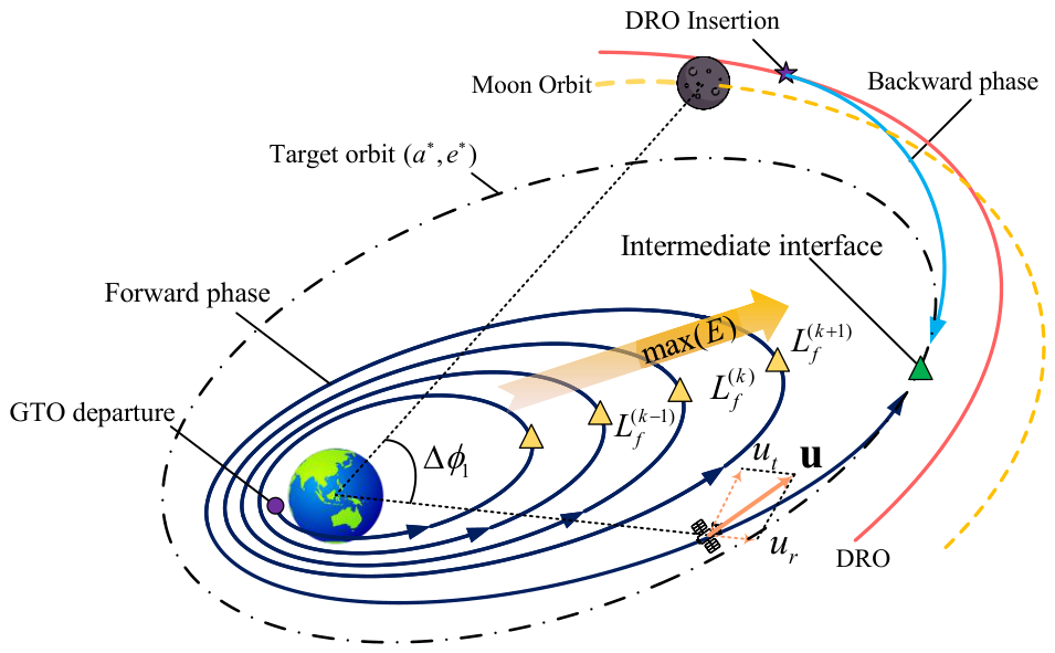
Since practical DROs are typically designed in the Earth–Moon orbital plane, only in-plane motion is considered. The initial GTO is assumed to be coplanar with the lunar orbital plane so that the forward phase can focus on the essential task of raising orbital energy rather than spending control authority on plane changes. A schematic of the transfer initialization strategy is shown in Figure 1. The forward phase is described in the geocentric inertial frame, and the intermediate interface is introduced to connect the long Earth-centered spiral-out process with the subsequent backward initialization from the DRO side. In this way, the forward initialization plays a clear physical role: it guides the trajectory toward a high-energy region that is more suitable for later matching with the lunar-side transfer arc, while still remaining numerically simple enough to support robust continuation.

2.1. Dynamics and Costate Equations

This subsection introduces only the dynamical and optimality structure needed for the forward auxiliary problem. The objective here is to generate a numerically robust family of Earth-centered extremals that can later seed the fixed- ( a , e ) minimum-time problem, rather than to reproduce the full coupled mission model at this stage.
For the planar orbital dynamics, the state vector is defined as
x = p f g L m T ,
where the first four components correspond to the planar MEEs [ p , f , g , L ] T and the last component is the spacecraft mass m. The planar MEEs are related to the classical orbital elements by
p = a ( 1 e 2 ) , f = e cos ω , g = e sin ω , L = ω + θ ,
with a, e, ω , and  θ denoting the semi-major axis, eccentricity, argument of periapsis, and true anomaly, respectively [28]. Hence,
e = f 2 + g 2 , a = p 1 f 2 g 2 .
Introducing
w = 1 + f cos L + g sin L , r = p w ,
the planar dynamics can then be expressed in control-affine form as
x ˙ 1 : 4 = A ( x ) + B ( x ) T max m u + a m ( x , t ) , m ˙ = T max I s p g r ,
where x 1 : 4 denotes the first four components of x corresponding to the planar MEE, u = [ u r , u t ] T is the in-plane thrust-direction unit vector with u = 1 , and T max / m is the maximum thrust acceleration. Here, a m ( x , t ) = [ a m , r , a m , t ] T denotes the lunar disturbing acceleration resolved in the local radial–transverse frame. The normalized maximum thrust coefficient is defined by
T max = 2 η P 0 I s p g r ,
where η is the propulsion efficiency, P 0 is the available power, I s p is the specific impulse, and  g r is the normalized reference gravitational acceleration [29].
In Equation (5), a m ( x , t ) denotes the lunar gravitational perturbation expressed in the planar MEE coordinates. It is retained in the notation to keep the connection with the later fully coupled formulation explicit, but during the first-stage initialization we set this perturbation term to zero. The reason is physical as well as numerical: in the long initial spiral, the gross effect to be captured is the monotonic increase in Earth-centered orbital energy under low thrust, whereas introducing lunar perturbations at this stage would substantially complicate the costate structure without changing that dominant trend. The resulting two-body geocentric model therefore serves as a deliberate auxiliary problem that preserves the main energy-raising behavior while remaining suitable for robust indirect continuation.
The drift vector and control matrix are given by
A ( x ) = 0 0 0 μ p 3 w 2 , B ( x ) = p μ 0 2 p w sin L ( 1 + w ) cos L + f w cos L ( 1 + w ) sin L + g w 0 0 ,
where μ denotes the normalized geocentric gravitational parameter. To maintain normalization consistency with the subsequent Earth–Moon transfer phase, we set μ = μ E / ( μ E + μ M ) , so that the total Earth–Moon gravitational parameter is normalized to unity.
A throttle variable may in principle be introduced in [ 0 , 1 ] . However, for the minimum-time problem considered later, the PMP implies that the thrust magnitude saturates at its upper bound throughout [30]. The forward phase is therefore written directly in the full-thrust form of Equations (5)–(7).
To unify the subsequent formulations, the Hamiltonian is written as
H = + λ 1 : 4 T A ( x ) + B ( x ) T max m u λ m T max I s p g r ,
where = 0 for the fixed-section maximum-energy problem and = 1 for the minimum-time problem, λ 1 : 4 = [ λ p , λ f , λ g , λ L ] T , and  λ m is the mass costate. The full costate vector is defined as λ = [ λ 1 : 4 , λ m ] T . Since u enters the Hamiltonian linearly and is constrained by u = 1 , the optimal control direction is
u * = [ u r * , u t * ] T = B T ( x ) λ 1 : 4 B T ( x ) λ 1 : 4 .
The costate equations follow from
λ ˙ = H x .
The costate equations are generated through automatic differentiation of the Hamiltonian and are omitted here for brevity. For many-revolution continuation, the main numerical difficulty is that the costates associated with the orbital-shape variables can grow at very different rates as the orbit expands. To prevent this scale separation from overwhelming the shooting iteration, the first three costates are scaled as
λ ˜ p = p 2 λ p , λ ˜ f = p λ f , λ ˜ g = p λ g .
The corresponding inverse transformation and the chain-rule form of the scaled costate dynamics, together with the detailed construction of the initial-costate parameterization, are provided in Appendix A. For the shooting formulation, define the scaled initial costate vector as
λ ˜ = λ ˜ p λ ˜ f λ ˜ g λ L λ m T = λ n l , l = 1 ,
where λ n denotes the magnitude of the scaled costate and l R 5 denotes its direction vector [19,31]. The shooting unknowns are therefore represented by the five components of l together with λ n , which provides a compact and numerically convenient parameterization for the continuation and shooting procedures.

2.2. Maximum-Energy Problem Continuation

The multi-revolution low-thrust problem admits multiple extremal branches, and direct shooting for a terminally constrained minimum-time formulation is highly sensitive to the initial costate guess. The role of the maximum-energy continuation introduced here is to select, from these competing extremals, the forward branch that most consistently increases Earth-centered orbital energy and therefore drives the trajectory toward a high-apogee, near-escape region. In physical terms, this continuation follows the Earth-centered spiral-out family that is most useful for later connection with the lunar-side transfer, rather than attempting to guess the final minimum-time branch directly. The geocentric-specific orbital energy in a planar MEE is
E = μ ( f 2 + g 2 1 ) 2 p .
The first forward subproblem is posed as
min J E = E x ( t f )
subject to Equations (5)–(10), the prescribed initial state x ( 0 ) = x 0 , and the terminal section
L ( t f ) = L f .
Here, t f is not prescribed a priori; instead, it is the first time at which the trajectory reaches the section L = L f . In the planar setting, L is equivalent to the phase angle in the chosen frame, so fixing L f amounts to advancing the trajectory by successive half-revolution events rather than by prescribing an absolute terminal time. This choice has a clear physical interpretation: as the spiral expands and the orbital period changes continuously, equal increments in time no longer correspond to comparable orbital progress, whereas equal increments in L continue to represent comparable geometric events along the outward spiral. The fixed-section formulation therefore provides a much more reliable continuation parameter for tracing the same high-energy branch over many revolutions.
For this problem, = 0 in Equation (8), and the optimal control direction is still given by Equation (9). For the maximum terminal-energy problem, the performance index is of Mayer type, Equation (14). According to the PMP, the terminal costates satisfy the transversality condition
λ ( t f ) = ( E ) x f .
Taking the partial derivatives yields
λ p ( t f ) = μ 2 p f 2 f f 2 + g f 2 1 , λ f ( t f ) = μ f f p f , λ g ( t f ) = μ g f p f .
Using the scaling relations summarized in Appendix A, the terminal conditions for the scaled costates become
R E = λ ˜ p ( t f ) μ 2 f f 2 + g f 2 1 λ ˜ f ( t f ) + μ f f λ ˜ g ( t f ) + μ g f λ m ( t f ) H E ( t f ) = 0 .
The free-final-time condition H E ( t f ) = 0 follows from the fact that the terminal event is a fixed section rather than a prescribed final time, forming a TPBVP that can be solved by the shooting method. To progressively increase the number of revolutions, the terminal phase L f is used as the continuation parameter. In this way, each continuation step extends the same forward branch to the next apogee-type section, so the method does not search for a distant many-revolution solution in one attempt; instead, it incrementally pushes the spiral toward higher energy while preserving branch continuity. Starting from a half-revolution solution, a family of many-revolution extremals is obtained by continuation in the terminal section,
L f ( k ) = ( 2 k 1 ) π , k = 1 , 2 , , N
At each continuation step, the converged solution of the previous terminal section is used to construct the initial guess for the next one. Let ( k , ) denote the converged solution at the k-th continuation step, and let ( k + 1 , 0 ) denote the initial guess for the ( k + 1 ) -th continuation problem. The direction of the normalized costate vector is directly inherited from the previous solution,
l ( k + 1 , 0 ) = l ( k , ) .
The magnitude parameter λ n is predicted using the terminal transversality condition. Since the Hamiltonian system is homogeneous with respect to the costate variables, the extremal trajectory remains unchanged under a uniform scaling of the costates. Therefore, the magnitude can be corrected according to the terminal condition of the λ ˜ p component in Equation (18).
Let the subscript f denote the terminal state at the end of the k-th continuation step. The predictor for the costate magnitude is then written as
λ n ( k + 1 , 0 ) = λ n ( k , ) μ 2 f f ( k + 1 ) 2 + g f ( k + 1 ) 2 1 λ ˜ p , f ( k + 1 ) .
Here λ ˜ p , f ( k ) denotes the value of the scaled costate component λ ˜ p evaluated at the terminal point of the k-th continuation solution. This predictor preserves the costate direction while correcting only its magnitude to satisfy the terminal optimality trend of the next section. Numerically, this is effective because adjacent continuation solutions on the same branch usually differ more in scale than in orientation. Physically, it means that the continuation keeps following the same spiral-out mechanism of energy increase instead of jumping to a different extremal family. The resulting parameters [ l , λ n ] for each fixed terminal section L f therefore provide a consistent set of warm starts for the minimum-time forward problem formulated in the next subsection.

2.3. Fixed- ( a , e ) Time-Optimal Problem

The maximum-energy continuation identifies a forward branch with the correct energy-growth tendency, but it is not yet the final time-optimal Earth-centered arc used in the coupled problem. A second forward subproblem is therefore introduced to convert that high-energy branch into a terminally constrained minimum-time segment at a selected interface. In principle, a planar intermediate interface should be characterized by four orbital parameters, namely ( a , e , ω , θ ) . In the present problem, however, the interface is prescribed at the apogee, so the true anomaly is fixed by the terminal event as θ = ( 2 k + 1 ) π , k Z . The remaining angular parameter ω represents only the in-plane orientation of the osculating ellipse. Owing to the rotational symmetry of the planar two-body dynamics, varying ω does not change the size or shape of the optimal trajectory, but only rotates its overall orientation in the plane. Consequently, the mismatch in ω at the intermediate interface can be compensated by adjusting the initial orientation of the GTO orbit, so that the forward trajectory can be connected with the backward phase in a common geocentric frame. For this reason, the target parameters at the intermediate interface are chosen as ( a , e ) .
The energy-continuation family provides not only a consistent branch of costate solutions but also the corresponding semi-major axis and eccentricity at different revolution numbers. From this family, the pair ( a * , e * ) associated with the N-th apogee is selected to define the intermediate interface parameters for the subsequent minimum-time problem, and the corresponding time is denoted by t I . In this sense, the fixed- ( a , e ) problem serves as a bridge: it takes the physically meaningful high-energy orbit identified by the continuation and enforces the time-optimality conditions needed for a later match with the backward arc.
To define the apogee event in the MEE variables with Equation (2), consider the scalar function
γ ( x ) = e sin θ = e cos ω sin ( ω + θ ) e sin ω cos ( ω + θ ) = f sin L g cos L .
Hence, γ ( x ) = 0 is exactly equivalent to an apsidal event. The apogee is identified by a sign crossing of γ ( x ) from positive to negative, which corresponds to an outbound-to-inbound transition of the radial motion. Let t A ( N ) denote the time of the N-th such crossing.
The terminally constrained forward problem is then stated as
min J = 0 t I 1 d t = T 1
subject to Equation (5) together with the corresponding scaled costate dynamics summarized in Appendix A,
x ( t 0 ) = x 0 ,
and
a ( t I ) = a * , e ( t I ) = e * , t I = t A ( N ) .
For this problem, = 1 in Equation (8), so that
H 1 = 1 + λ T A ( x ) + B ( x ) T max m u λ m T max I s p g r ,
with the same optimal direction law as in Equation (9). The free-final-time condition is
H 1 ( t I ) = 0 .
The terminal constraints can be collected as
Φ 1 ( x ( t I ) ) = a ( x ( t I ) ) a * e ( x ( t I ) ) e * γ ( x ( t I ) ) = 0 ,
where
a = p D , e = f 2 + g 2 , D = 1 f 2 g 2 .
If the terminal multipliers were introduced explicitly, the transversality condition would read
λ ( t I ) = G 1 ν 1 , ν 1 R 3 ,
where G 1 R 5 × 3 is the matrix of terminal constraint gradients,   
G 1 = a X , e X , ϕ X t = t I = 1 D 0 0 2 p f D 2 f e sin L 2 p g D 2 g e cos L 0 0 f cos L + g sin L 0 0 0 t = t I .
A direct shooting implementation based on Equation (30) would require the additional unknown Lagrange multipliers ν . To avoid these extra guesses, let N 1 R 5 × 2 be a basis of the null space of G 1 T . For the definition and construction of the null-space operator [32], see Appendix B.
N 1 = null G 1 T .
Since range ( G 1 ) is orthogonal to null ( G 1 T ) , Equation (30) is equivalent to
N 1 T λ ( t I ) = 0 ,
which eliminates the terminal multipliers without sacrificing the exact transversality condition. Using the scaled initial costate parameterization summarized in Appendix A, the shooting unknown can be written as
s for = l T λ n T R 6 .
The TPBVP shooting residual is
R for = a ( x ( t I ) ) a * e ( x ( t I ) ) e * N 1 T λ ( t I ) H 1 ( t I ) l 1 = 0 , R for R 6
which defines six scalar equations for the six unknowns in s for . Specifically, the first two residual components jointly enforce the prescribed terminal orbital-shape conditions at the N-th apogee, namely the semi-major axis and eccentricity constraints. The third residual is a two-dimensional null-space transversality condition, and  N 1 T λ ( t I ) contains two scalar components. This residual enforces the terminal costate transversality condition on the constrained terminal manifold. The fourth residual imposes the free-final-time condition associated with the terminal apogee event. The last residual normalizes the initial costate direction and removes the trivial scaling freedom of the costates.
The role of this subsection should therefore be emphasized clearly. The fixed- ( a , e ) problem is not introduced as an independent final mission optimization problem. Rather, it converts the high-energy continuation family into a forward arc that already satisfies the minimum-time optimality structure at the selected interface, thereby providing a robust bridge between the energy-growth initialization and the later coupled GTO-to-DRO problem.

3. DRO-Insertion Initialization

Due to the change in the dominant gravitational regime, the DRO insertion phase is modeled in the planar Earth–Moon CRTBP. Since the terminal state is constrained on the target DRO and the insertion phase along the DRO is free, this phase is formulated in a backward manner. The main advantage of this construction is that the most restrictive local structure of the second phase is defined at the target end: the terminal geometry on the DRO, the insertion phase, and the associated transversality conditions are all prescribed there more naturally than at the intermediate interface. By propagating backward from the DRO insertion point to the interface specified by the fixed orbital elements ( a * , e * ) , the method first anchors the locally admissible terminal-insertion branch and then transfers this information back to the interface. In this way, the backward subproblem captures the local dynamics of precise DRO insertion, while the forward subproblem remains focused on the long-duration Earth-centered orbit-raising process.

3.1. Target DRO and Phase Parameterization

DROs form a family of stable periodic orbits around the smaller primary in the CRTBP. In the Earth–Moon system, lunar DROs appear as retrograde periodic motions around the Moon in the synodic frame. In this work, a representative 2:1 lunar DRO is selected as the target orbit, where “2:1” denotes the ratio between the lunar orbital period and the DRO period [33]. Let the planar DRO solution be denoted by
χ D ( t ) = x D ( t ) y D ( t ) v x , D ( t ) v y , D ( t ) T , χ D ( t + T D ) = χ D ( t ) ,
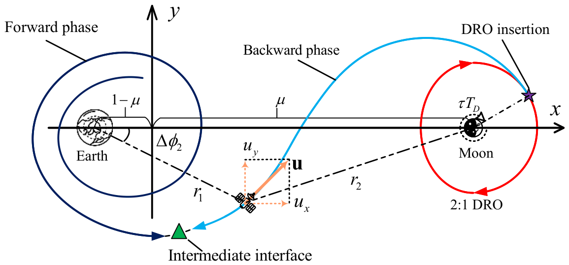
where T D is the DRO normalized period. The geometry of the selected lunar DRO is illustrated in Figure 2, which provides a reference view of the target orbit in the synodic frame.
Since different insertion phase locations on the DRO can significantly affect the transfer time from the intermediate point to the target orbit, the DRO phase is treated as an optimization variable rather than being fixed a priori. Let τ denote the phase parameter of the target DRO. To avoid discontinuity at the periodic wrapping point and to allow smooth local variations during the optimization process, τ is defined over
τ [ 0 , 2 ] ,
with τ = 1 chosen as the reference phase corresponding to the far Earth side point of the target DRO. The associated physical phase time is written as
t τ = τ T D , χ D ( τ ) = χ D ( t ) | t = τ T D .

3.2. Fixed- ( a , e ) Time-Optimal Problem in CRTBP

Let the planar state vector of the insertion leg be defined as
X ( t ) = x ( t ) y ( t ) v x ( t ) v y ( t ) m ( t ) T .
With μ denoting the normalized Earth mass parameter and 1 μ the normalized Moon mass parameter, the Earth and Moon are located at ( ( 1 μ ) , 0 ) and ( μ , 0 ) , respectively. Therefore, the distances to the Earth and Moon are
r 1 = ( x + 1 μ ) 2 + y 2 , r 2 = ( x μ ) 2 + y 2 .
The planar CRTBP low-thrust dynamics are written as
x ˙ = v x , y ˙ = v y ,
v ˙ x = 2 v y + x μ ( x + 1 μ ) r 1 3 ( 1 μ ) ( x μ ) r 2 3 + T max m u x ,
v ˙ y = 2 v x + y μ y r 1 3 ( 1 μ ) y r 2 3 + T max m u y ,
m ˙ = T max I s p g r .
The thrust direction is
u = u x u y T , u = 1 .
The objective of the insertion phase is also minimum transfer time
min J = t f t I 1 d t = T 2
The Hamiltonian is
H 2 = 1 + λ x v x + λ y v y +   λ v x 2 v y + x μ ( x + 1 μ ) r 1 3 ( 1 μ ) ( x μ ) r 2 3 + T max m u x +   λ v y 2 v x + y μ y r 1 3 ( 1 μ ) y r 2 3 + T max m u y λ m T max I s p g r .
The costate equations satisfy
Λ ˙ = H X .
The optimal thrust direction is
u * = 1 λ v x 2 + λ v y 2 λ v x λ v y .

3.3. Backward Shooting Formulation and Initialization

Using the state vector introduced in the previous subsection,
X ( t ) = x ( t ) y ( t ) v x ( t ) v y ( t ) m ( t ) T ,
the terminal state on the target DRO is parameterized by the phase variable τ as
X f = χ D ( τ ) m f , χ D ( τ ) = x D ( τ ) y D ( τ ) v x , D ( τ ) v y , D ( τ ) T ,
Here m f is the terminal mass at the DRO insertion point, which needs to be provided as an initial guess. Therefore, the corresponding terminal costate is prescribed as
λ m , f = 0 .
Starting from X f and the corresponding terminal costate, the state and costate dynamics are integrated backward from the DRO insertion point to the intermediate interface with state X I and costate Λ I .
To express the interface conditions in the CRTBP rotating frame, consider the Earth-centered inertial position and velocity. The apogee event can be equivalently identified by the vanishing of the Earth-centered radial velocity. Therefore, instead of introducing the angular event explicitly, the apogee condition is detected through the inner product of the position and velocity vectors in the Earth-centered synodic coordinate system,
r E I = R ( Δ ϕ ) x + 1 μ y , v E I = R ( Δ ϕ ) v x y v y + x + 1 μ ,
where R ( Δ ϕ ) is the planar rotation matrix and Δ ϕ is the synodic-to-inertial rotation angle, which is also the Moon’s phase angle in the Earth-centered inertial frame. Since R T ( Δ ϕ ) R ( Δ ϕ ) = I , where I denotes the identity matrix, the event condition is invariant under phase rotation. Thus,
Γ 2 ( X ) : = r E I T v E I = x + 1 μ y v x y v y + x + 1 μ = ( x + 1 μ ) v x + y v y .
Accordingly, the intermediate interface constraints are written as
Φ 2 ( X ( t I ) ) = a ( X I ) a * e ( X I ) e * Γ 2 ( X I ) m ( t I ) m * = 0 .
where m * is directly inherited from the terminal mass of the preceding GTO-raising phase to ensure continuity between the two phases.
The osculating semi-major axis and eccentricity in the Earth-centered inertial system can be expressed directly in terms of the CRTBP state as:
r E = ( x + 1 μ ) 2 + y 2 , v E 2 = ( v x y ) 2 + ( v y + x + 1 μ ) 2 ,
h E = ( x + 1 μ ) ( v y + x + 1 μ ) y ( v x y ) ,
E E = 1 2 v E 2 μ r E ,
a ( X ) = μ 2 E E ,
e ( X ) = 1 + 2 E E h E 2 μ 2 .
where r E denotes the Earth-centered distance, v E denotes the magnitude of the Earth-centered inertial velocity, h E denotes the corresponding specific angular momentum, and  E E denotes the specific mechanical energy in the Earth-centered two-body problem. In the backward propagation, the integration is terminated when the event condition Γ ( X ( t I ) ) = 0 is satisfied. During the backward propagation, the apse intersection is detected automatically, so the flight time of this phase does not need to be treated as an additional shooting variable.
The Jacobian of the constraint vector with respect to the state is denoted by
G 2 = Φ 2 X t = t I R 4 × 5 .
The explicit expressions of the partial derivatives involved in G 2 are summarized in Appendix C. Since the interface is defined by the constrained manifold Φ 2 ( X ) = 0 , the associated transversality condition is imposed through the null space of G 2 , similar to the approach used in Section 2.3, where the null space of the Jacobian was also employed.
N 2 = null ( G 2 T ) R 1 × 5 ,
then the interface transversality condition is
N 2 T Λ I = 0 ,
where Λ I denotes the costate vector at the intermediate point.
With λ m , f = 0 already prescribed, the unknown vector of the backward shooting TPBVP is reduced to
s back = λ x , f λ y , f λ v x , f λ v y , f m f τ T R 6 .
For a trial s back , the terminal state and costate at the DRO insertion point are initialized as
X f = χ D ( τ ) m f , Λ f = λ x , f λ y , f λ v x , f λ v y , f T , λ m , f = 0 .
and then propagated backward until the event condition (54) is reached. The free final time condition at the DRO insertion point is
H 2 ( t f ) = 0 .
Moreover, since the insertion point is free to move along the target DRO, the corresponding phase transversality condition is
Λ f T χ D τ = 0
Since the terminal state on the target DRO is parameterized by Equation (38), its derivative with respect to the phase parameter is given by
χ D τ = T D χ ˙ D ( t ) | t = τ T D
where T D is the period of the target DRO. Therefore, the phase transversality condition can be equivalently written as
Λ f T T D χ ˙ D ( t ) | t = τ T D = 0 .
Collecting all residual components, the backward TPBVP shooting function is finally written as
R back = a ( X I ) a * e ( X I ) e * m ( t I ) m * N 2 T Λ I H 2 ( t f ) Λ f T T D χ ˙ D ( τ T D ) = 0 , R back R 6
which defines six scalar equations for the six unknowns in s back . Specifically, the first two residual components jointly enforce the prescribed interface orbital-shape conditions, namely the semi-major axis and eccentricity constraints at the intermediate point. The third residual enforces the continuity of the spacecraft mass at the interface by requiring the backward terminal mass at t I to match the prescribed value m * inherited from the forward phase. The fourth residual is a one-dimensional null-space transversality condition, since N 2 R 1 × 5 , and it imposes the interface costate transversality on the constrained manifold. The fifth residual imposes the free-final-time condition at the DRO insertion point. The last residual enforces the phase transversality condition associated with the freedom of the terminal point to move along the target DRO.
To generate a reliable initial guess for s back , the backward local optimal-control problem is first solved by a Legendre–Gauss–Radau pseudospectral transcription implemented in GPOPS [34]. This choice is particularly suitable for the present DRO-insertion segment because the arc is comparatively short, the terminal manifold on the target DRO is explicitly parameterized by ( m f , τ ) , and the local trajectory does not contain the many-revolution structure that makes direct transcription less attractive in the first phase. Therefore, for this backward arc the direct method has a clear practical advantage: it can rapidly capture the correct local insertion geometry and provide a feasible terminal branch without requiring a delicate a priori guess of the continuous costates [35]. This discrete solution is then used to supply the initial neighborhood required by the subsequent indirect refinement.
The role of the pseudospectral solution is not to replace the subsequent indirect method, but to provide a high-quality initialization for it. Following the costate-estimation idea of Benson [36], the key point is that, with a proper pseudospectral discretization, the Karush–Kuhn–Tucker (KKT) conditions of the resulting nonlinear programming problem are consistent with the discretized first-order necessary conditions of the original continuous optimal-control problem. Consequently, the NLP multipliers can be interpreted as discrete covectors and used to construct an estimate of the continuous costates at the collocation points and the endpoints. In the notation of the costate mapping theorem, this relation can be written schematically as
Λ k ps = Λ ˜ k w k + Λ ˜ f , Λ f ps = Λ ˜ f ,
where Λ ˜ k denotes the KKT multipliers associated with the defect constraints, Λ ˜ f denotes the endpoint multiplier, and  w k is the quadrature weight. Equation (71) expresses the essential meaning of covector mapping: the multiplier information returned by the direct NLP solver provides a consistent approximation of the continuous-time adjoint variables.
Accordingly, after the pseudospectral problem is solved, the mapped terminal covector is used to initialize the four terminal costate components in Equation (64), while the terminal mass and the DRO phase are taken directly from the same discrete solution. The resulting initial guess is written as
s back ( 0 ) = λ x , f ps λ y , f ps λ v x , f ps λ v y , f ps m f ps τ ps T .
It should be emphasized that the pseudospectral solution remains a mesh-dependent discrete approximation and is used here only as an initializer for the indirect TPBVP rather than as the final solution of the backward phase. For the present backward arc, the indirect shooting refinement does not require the direct solution to satisfy the continuous optimality conditions with very high accuracy. Instead, it mainly requires the pseudospectral seed to capture the correct insertion branch, the terminal phase on the DRO, the terminal mass level, and the main local lunar-approach geometry, so that the mapped terminal costates lie within a reasonable convergence neighborhood of the backward TPBVP. Under this condition, the subsequent shooting iteration can usually absorb moderate discretization and optimality errors in the direct seed and rapidly converge to the continuous indirect solution. On the other hand, if the pseudospectral solution is too coarse, converges to an incorrect insertion branch, or does not represent the local terminal geometry adequately, then the mapped covector may fall outside the attraction region of the shooting problem and the refinement may become unreliable. Once s back ( 0 ) is obtained, the shooting equations in Equation (70) are solved to recover a continuous solution that satisfies the Hamiltonian condition, the interface transversality condition, and the DRO phase transversality condition with higher accuracy. In this way, the direct method provides an efficient local initializer, whereas the indirect method restores the continuous first-order optimality conditions in the final refinement.

4. Solution of the Fully Coupled Optimization Problem

The overall transfer optimization is performed in two successive steps. First, with the locally optimal subproblem solutions obtained in Section 2 and Section 3, the interface orbital parameters are adjusted so that the forward Earth-centered arc and the backward DRO-insertion arc meet on a common handover orbit in an optimality-consistent manner. In geometric terms, the pair ( a * , e * ) determines the size and shape of this intermediate geocentric handover orbit. Changing these two parameters moves the interface orbit in the ( a , e ) plane, which changes how the total transfer burden is distributed between the forward orbit-raising phase and the backward DRO-insertion phase. This outer-level step therefore identifies a physically balanced interface configuration and yields a numerically robust initial guess for the coupled problem. Second, using this guided initial solution, the lunar phase evolution and the long-term lunar gravitational perturbation are reintroduced into the GTO-raising phase, and the forward and backward phases are assembled into a fully coupled multi-phase optimal-control problem for further refinement.

4.1. Two-Level Optimization Framework for the Coupled Problem

As established in Section 2 and Section 3, for suitable prescribed interface orbital parameters ( a * , e * ) , the forward GTO-raising subproblem and the DRO backward transfer subproblem can be solved independently, yielding two locally time-optimal trajectories with flight times T 1 ( a * , e * ) and T 2 ( a * , e * ) , respectively. The present subsection therefore reduces the two-phase construction to an outer-level composition problem in which the common handover orbit is adjusted until the two local phases are matched in a first-order optimal sense. The corresponding total performance index is
min T sum ( a * , e * ) = T 1 ( a * , e * ) + T 2 ( a * , e * ) .
Here, T sum denotes the total flight time of the composed two-phase trajectory. Physically, ( a * , e * ) specify the common handover orbit on which the spacecraft leaves the Earth-centered spiral and enters the lunar-side insertion leg. If this handover orbit is chosen too low in energy, the forward phase is easier but the backward phase becomes more demanding; if it is chosen too high, the opposite tradeoff occurs. The role of the outer iteration is therefore to move the handover orbit in the ( a , e ) plane until these competing marginal time costs are balanced, rather than to re-solve the full coupled problem directly at the outset.
For the forward subproblem, the interface conditions are written as
h 1 x I = a ( x I ) a * e ( x I ) e * = 0 .
For the backward subproblem, the same physical interface is expressed in its own state representation as
h 2 X I = a ( X I ) a * e ( X I ) e * = 0 .
Here, the lowercase vector x I denotes the interface state obtained from the forward GTO-raising phase, where the state is expressed in the planar MEE variables. Accordingly, a ( x I ) and e ( x I ) are evaluated from the MEE relations given in Equation (29). By contrast, the uppercase vector X I denotes the interface state obtained from the backward DRO-transfer phase, where the state is expressed in the planar Earth–Moon CRTBP variables. In this case, a ( X I ) and e ( X I ) are evaluated from Equations (59) and (60), respectively. Therefore, x I and X I represent the same physical interface orbit, but in two different state representations.
It should be emphasized that the two local subproblems are formulated with different dynamical models and different state coordinates. Consequently, direct element-wise continuity cannot be imposed on the costates at the phase boundary. Instead, the coupling is established through the Lagrange multipliers associated with the same physical interface constraints,
ν 1 = ν 1 , a ν 1 , e , ν 2 = ν 2 , a ν 2 , e ,
which are coordinate-independent first-order sensitivity quantities with respect to the common parameters ( a * , e * ) . More specifically, ν 1 , a and ν 1 , e describe how the locally optimal flight time of the forward phase varies under small shifts of the handover orbit in the ( a , e ) plane, while ν 2 , a and ν 2 , e play the same role for the backward phase.
According to Equation (30), once the interface costate λ I of the first phase has been obtained, the corresponding multiplier vector ν 1 can be uniquely recovered through the associated constraint-gradient mapping at the intermediate interface, namely
ν 1 = G 1 T G 1 1 G 1 T λ I .
In the same manner, after obtaining the interface costate of the second phase, the corresponding multiplier vector can be recovered as
ν 2 = G 2 T G 2 1 G 2 T Λ I .
Therefore, ν 1 and ν 2 are not introduced as additional independent variables, but are directly computed from the costates at the intermediate interface.
After the two local subproblems have been solved, all other local constraints, including the dynamics, boundary conditions, transversality conditions, and the local apogee event constraint, are already satisfied. Hence, if the interface parameters are perturbed by
δ p = δ a * δ e * ,
the corresponding first-order variations in the two local flight times are contributed to only by the interface constraints, namely,
δ T 1 = ν 1 T δ p , δ T 2 = ν 2 T δ p .
Therefore, for  T sum , its first-order variation is
δ T sum = ( ν 1 + ν 2 ) T δ p .
Since δ a * and δ e * are arbitrary, the first-order optimal condition requires
F ( a * , e * ) = ν 1 + ν 2 = ν 1 , a + ν 2 , a ν 1 , e + ν 2 , e = 0 ,
In other words, the stationarity condition F ( a * , e * ) = 0 means that the forward and backward phases exert equal and opposite first-order time sensitivities on the same handover orbit. If this balance is not satisfied, then a small displacement of the interface orbit can still reduce the total flight time by shortening one phase more than it lengthens the other. Only when these marginal time costs balance does the common interface represent a locally optimal handover orbit for the composed two-phase transfer.
To find a solution that makes F ( a * , e * ) = 0 , a finite-difference iteration is adopted. At the k-th outer iteration, let
p ( k ) = a , ( k ) e , ( k ) , F ( k ) = F a , ( k ) , e , ( k ) .
Using small perturbations δ a and δ e , the Jacobian of the residual is approximated by forward finite differences as
J F ( k ) F 1 ( a , ( k ) + δ a , e , ( k ) ) F 1 ( a , ( k ) , e , ( k ) ) δ a F 1 ( a , ( k ) , e , ( k ) + δ e ) F 1 ( a , ( k ) , e , ( k ) ) δ e F 2 ( a , ( k ) + δ a , e , ( k ) ) F 2 ( a , ( k ) , e , ( k ) ) δ a F 2 ( a , ( k ) , e , ( k ) + δ e ) F 2 ( a , ( k ) , e , ( k ) ) δ e .
The parameter correction is then computed from
Δ p ( k ) = J F ( k ) 1 F ( k ) ,
followed by the update
p ( k + 1 ) = p ( k ) + Δ p ( k ) .
Through this procedure, the interface orbital parameters are corrected step by step until Equation (81) is driven to zero, which is equivalent to satisfying the first-order stationarity condition of T sum with respect to ( a * , e * ) .
However, the present subsection adjusts only the interface orbital parameters ( a * , e * ) . The lunar phase continuity and the long-term lunar gravitational effect along the first phase are not yet enforced as part of the strict coupled optimization. The purpose of this intermediate step is therefore not to produce the final coupled optimum directly, but to isolate the dominant handover–orbit tradeoff before the remaining coupling effects are restored. Once the interface sensitivities have been balanced, the resulting two-phase construction already lies near a locally optimal transfer geometry and provides a much better initial guess for the final coupled shooting problem. Therefore, the solution obtained here is used as the initial iterate for Section 4.2, where the fully coupled optimal-control problem is reintroduced with lunar phase variation, first-phase lunar perturbation, and complete inter-phase coupling conditions.

4.2. Fully Coupled Indirect Shooting with Lunar-Phase Matching

Starting from the planar affine dynamics in Equation (5), the forward arc is augmented by the lunar phase ϕ , so that the state is extended from x to
x = p f g L m ϕ T .
Under the present nondimensionalization, the lunar angular rate is unity, i.e.,  ϕ ˙ = 1 . Accordingly, the time-dependent perturbation term a m ( x , t ) can be re-parameterized as a m ( x , ϕ ) .
Let
w = 1 + f cos L + g sin L , r = p w , Δ ϕ = L ϕ .
In the local radial–transverse frame, define the unit vector pointing from the Earth to the Moon as
e M = cos Δ ϕ sin Δ ϕ ,
and the spacecraft-to-Moon relative position vector as
ρ = r 0 e M = r cos Δ ϕ sin Δ ϕ , ρ = ρ = r 2 2 r cos Δ ϕ + 1 .
The lunar disturbing acceleration is then written as the direct lunar attraction on the spacecraft minus the lunar attraction on the Earth. Therefore,
a m ( x , ϕ ) = ( 1 μ ) ρ ρ 3 e M = ( 1 μ ) r cos Δ ϕ sin Δ ϕ r 2 2 r cos Δ ϕ + 1 3 / 2 + cos Δ ϕ sin Δ ϕ .
This form makes the perturbation depend explicitly on the instantaneous Earth–spacecraft–Moon geometry, which is exactly the quantity required later in the interface phase matching.
Accordingly, Equation (26) is updated to
H 1 = H 1 + λ T B ( x ) a m ( x , ϕ ) + λ ϕ ,
where H 1 is the Hamiltonian defined in Equation (26). The augmented costate equations are still obtained from Equation (10) after including ϕ in the state, and the optimal thrust direction remains Equation (9). Since ϕ 0 is free to guess, its conjugate transversality condition is
λ ϕ ( t 0 ) = 0 ,
To derive the initial phase ϕ 0 , the following interface phase differences are introduced as:
Δ ϕ 1 = mod L I ϕ I + π , 2 π π , Δ ϕ 1 ( π , π ] ,
and
Δ ϕ 2 = atan2 ( y I , x I + 1 μ ) , Δ ϕ 2 ( π , π ] ,
where atan2 ( · , · ) denotes the four-quadrant inverse tangent. Thus, Δ ϕ 1 and Δ ϕ 2 represent the same Moon-relative geometric angle at the interface in the two distinct coordinate systems, as indicated in Figure 1 and Figure 2.
Since the phase evolution satisfies
ϕ I = ϕ 0 + T 1 ϕ ˙ ,
one has
ϕ 0 = L I Δ ϕ 1 T 1 ϕ ˙ .
Therefore, using the initial values obtained from the two subproblems and enforcing the interface-phase matching at the initialization level, i.e.,
Δ ϕ 1 * = Δ ϕ 2 * ,
a consistent initial guess for the coupled shooting problem is given by
ϕ 0 ( 0 ) = L I * Δ ϕ 2 * T 1 * ϕ ˙ .
In the normalized Earth–Moon system adopted here, ϕ ˙ = 1 .
Compared with Equations (28) and (55), the coupled interface is defined on the common quantities ( a , e , m ) , the apsidal constraint, and the Moon-relative phase. Let the forward and backward interface states be
x I = p I f I g I L I m I ϕ I T , X I = x I y I v x , I v y , I m I T .
For the GTO-raising arc, according to Equation (22), define
Γ 1 ( x ) = r E I T v E I = μ p w γ ( x ) = μ p w f sin L g cos L ,
so that Γ 1 = 0 defines the same apsidal section as γ = 0 , but with the physically consistent radial-velocity scaling required in the interface multiplier matching.
Define the two interface constraint vectors as
Ψ 1 ( x I ) = a ( x I ) e ( x I ) Γ 1 ( x I ) m ( x I ) Δ ϕ 1 ( x I ) , Ψ 2 ( X I ) = a ( X I ) e ( X I ) Γ 2 ( X I ) m ( X I ) Δ ϕ 2 ( X I ) .
The explicit continuity conditions retained in the shooting residual are
a ( x I ) a ( X I ) = 0 , e ( x I ) e ( X I ) = 0 , m ( x I ) m ( X I ) = 0 , Δ ϕ 1 Δ ϕ 2 = 0 .
The apsidal condition does not appear as an additional explicit residual because both arcs are already terminated on the apogee section, but it remains part of the interface manifold and must therefore be retained in the costate linkage.
The corresponding Jacobians are written as
G 1 = Ψ 1 x t = t I R 5 × 6 , G 2 = Ψ 2 X t = t I R 5 × 5 .
Here G 1 is obtained from the forward-interface Jacobian in the previous subsection after replacing γ by Γ 1 and appending the phase row, whereas G 2 is the corresponding Jacobian for the backward CRTBP interface constraints. The only new phase derivatives are
Δ ϕ 1 x = 0 0 0 1 0 1 , Δ ϕ 2 X = y I ρ I 2 x I + 1 μ ρ I 2 0 0 0 ,
where
ρ I 2 = ( x I + 1 μ ) 2 + y I 2 .
Using the same null-space elimination as in the previous sections, define
G all = ( G 1 ) T ( G 2 ) T R 11 × 5 , N all = null G all T R 11 × 6 ,
so that the interface costate linkage is imposed by
N all T λ I Λ I = 0 ,
where λ I R 6 and Λ I R 5 are the forward and backward interface costates, respectively. The terminal insertion conditions of the backward arc remain those given previously, namely H 2 ( t f ) = 0 and Equation (69).
Using the same scaled initial-costate parameterization as Equations (34) and (67), then the complete shooting vector is
s all = l 0 λ n , 0 ϕ 0 Λ f m f τ f T R 13
The initial guess for the shooting iteration is entirely provided by the bidirectional initialization framework developed in Section 4.1, and the fully coupled shooting residual is   
R all = a ( x I ) a ( X I ) e ( x I ) e ( X I ) m ( x I ) m ( X I ) Δ ϕ 1 Δ ϕ 2 N all T λ I Λ I l 0 1 Λ f T T D χ ˙ D ( τ f T D ) H 2 ( t f ) , R all R 13 .
The first two residual components jointly enforce the continuity of the interface orbital shape, namely the semi-major axis and eccentricity, between the forward and backward phases. The third residual enforces the continuity of the spacecraft mass at the interface. The fourth residual enforces the continuity of the Moon-relative phase angle at the interface. The fifth residual is a six-dimensional null-space costate-linkage condition, since N all R 11 × 6 , and it imposes the transversality-consistent linkage between the forward and backward interface costates on the common constrained manifold. The sixth residual normalizes the initial costate direction and removes the trivial scaling freedom of the forward-phase costates. The seventh residual enforces the phase transversality condition at the terminal point on the target DRO. The last residual imposes the free-final-time condition at the DRO insertion point. Equation (109) provides 13 scalar equations for the 13 unknowns in Equation (108), and therefore defines a square fully coupled shooting problem. Its solution yields a low-thrust transfer from GTO raising to DRO insertion that satisfies the first-order necessary conditions of optimality.

4.3. Algorithmic Framework of the Bidirectional Initialization Method

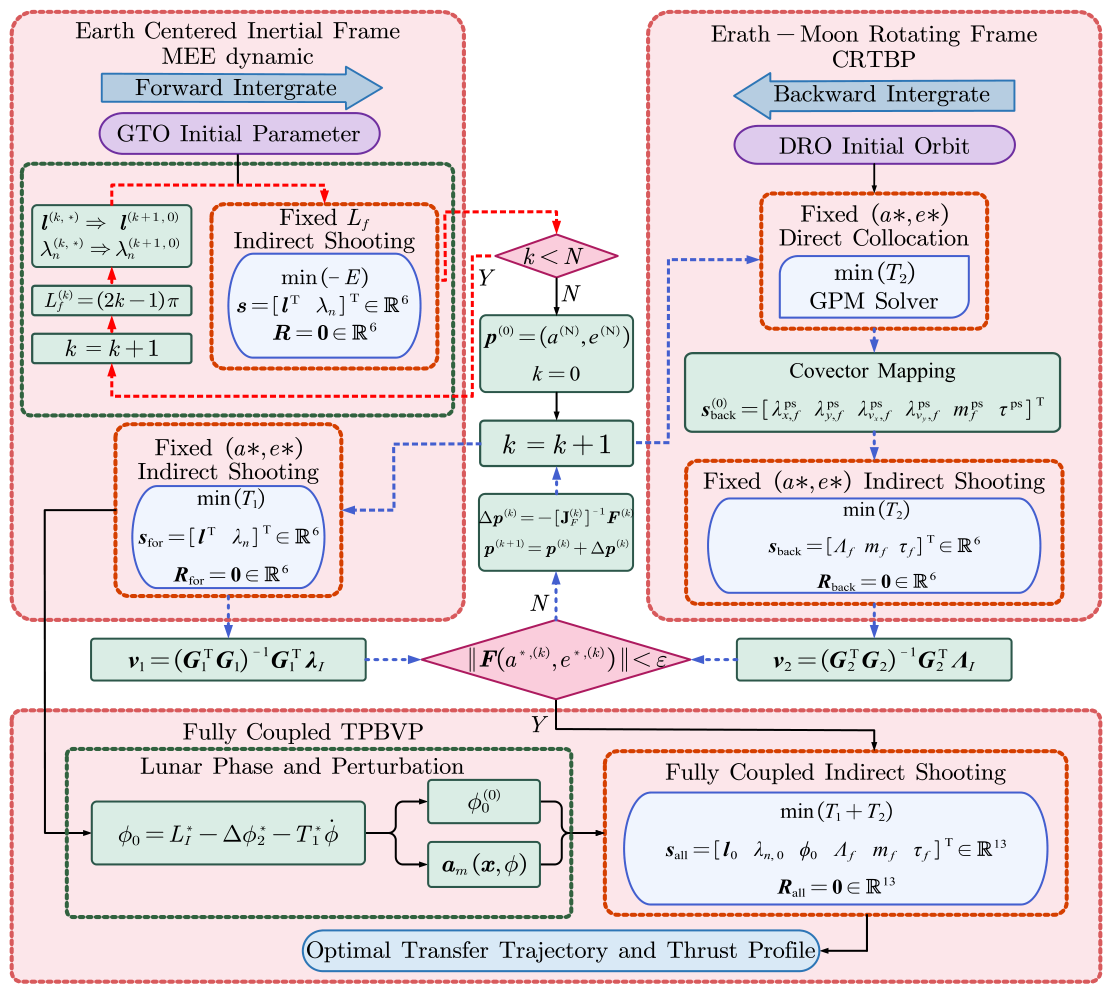
The overall solution procedure is summarized in Algorithm 1 and Figure 3. Here, the algorithm is intended as a concise companion to the flowchart, highlighting only the main computational stages of the proposed framework. The forward auxiliary solution is generated in the geocentric inertial model with planar modified equinoctial elements, where a fixed-section maximum-energy continuation is used to obtain a many-revolution orbit-raising family. A selected member of this family then initializes the fixed- ( a * , e * ) minimum-time forward subproblem. The backward auxiliary solution is constructed in the planar Earth–Moon CRTBP by propagating backward from the target DRO to the same intermediate interface. In this phase, a pseudospectral transcription and covector mapping are employed to provide a reliable initial guess for the backward indirect shooting variables. The two local solutions are coordinated by an outer-level iteration on the common interface parameters ( a * , e * ) , and the resulting bidirectional solution is finally refined by a fully coupled indirect shooting problem.
With the forward and backward subproblems solved for prescribed interface parameters ( a * , e * ) , the outer-level iteration moves the common handover orbit until the first-order time sensitivities of the two local phases are balanced. The converged bidirectional initialization therefore represents not merely a geometric connection of two trajectory segments, but a locally balanced state–costate neighborhood for the overall transfer. Based on this initialization, the lunar phase and the lunar perturbation on the forward arc are reintroduced, and the two phases are assembled into a fully coupled 13-dimensional indirect shooting problem. The converged solution of this final system yields the optimal transfer trajectory and the corresponding thrust profile.
Algorithm 1: Bidirectional Initialization and Fully Coupled Refinement
Aerospace 13 00429 i001

5. Numerical Results

All numerical examples in this section are carried out using the common normalization constants and propulsion parameters listed in Table 1 [37]. The normalized distance, time, and velocity units are denoted by LU, TU, and VU, respectively, where VU = LU / TU and TU = T E M / ( 2 π ) , with  T E M being the lunar orbital period.
The initial GTO state and the target DRO parameters are summarized in Table 2 [3,33]. The initial GTO state is specified at the perigee, with the initial argument of latitude set to zero. The initial GTO parameters are selected to represent a typical departure condition reported in the literature for rideshare or secondary-payload missions, in which the launch vehicle can only provide a limited injection energy and the remaining transfer must be completed by the spacecraft’s onboard low-thrust propulsion system. The initial perigee and apogee radii are denoted by [ r p , 0 , r a , 0 ] , equivalent to the MEEs. The target DRO is defined by its planar rotating-frame state at τ = 0 . In particular, a representative 2:1 lunar DRO is adopted because this orbit family is dynamically stable and is widely regarded as a practical staging orbit in cislunar mission design. Therefore, although the numerical example is not tied to a specific flight program, the adopted GTO–DRO configuration is intended to represent a practically meaningful low-thrust cargo-transfer scenario in cislunar space. All indirect TPBVP shooting equations are solved using MATLAB’s fsolve. All indirect TPBVP shooting equations are solved using the fsolve function in MATLAB R2024a. For the target 2:1 DRO, after one full-period solution is generated numerically, the DRO state and its time derivative at an arbitrary phase τ are evaluated by deval from the stored periodic solution at t τ = τ T D . This interpolation procedure is used in both the backward local shooting and the final fully coupled shooting computations.

5.1. Forward Continuation Characteristics and Interface-Parameter Selection

Before solving the fully coupled GTO-to-DRO shooting problem, the forward maximum-energy continuation is first examined, as it provides the reference orbit family for the subsequent bidirectional initialization. Its evolution with increasing energy also identifies a suitable intermediate interface reference for the later matching and full shooting procedure.
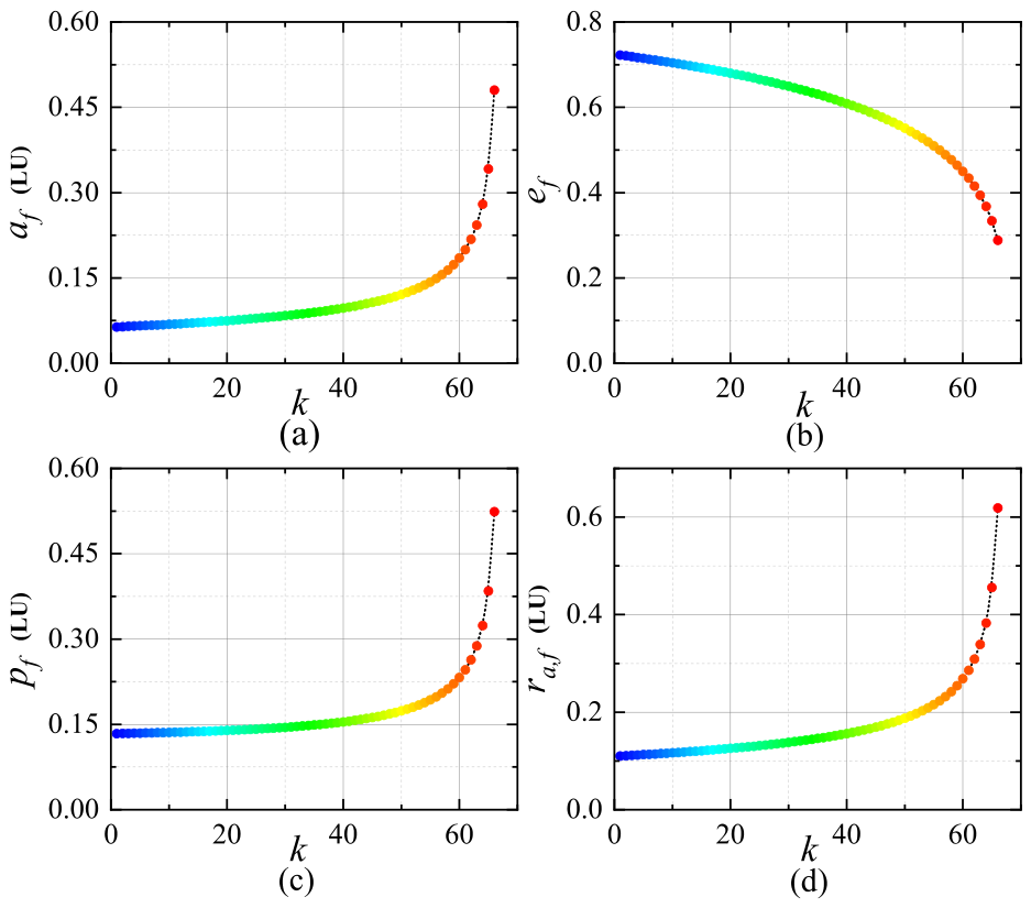
Figure 4 shows the evolution of the terminal orbital quantities along the forward maximum-energy continuation branch with respect to the continuation index k. As the continuation proceeds, the terminal orbit moves progressively toward a higher-energy regime, as reflected by the monotonic growth of the semi-major axis a f , semilatus rectum p f , and apogee radius r a , f , together with the gradual decrease in eccentricity e f . By the 66th apogee, the terminal orbit has already reached a f = 0.48048 ( LU ) , p f = 0.44049 ( LU ) , and r a , f = 0.61910 ( LU ) , while the eccentricity has decreased to e f = 0.28851 . This indicates that the forward branch has been lifted to a substantially higher orbital energy level and, at the same time, has become noticeably less eccentric. Such a trend is consistent with the expected behavior of continuous low-thrust orbit raising, in which the spacecraft gains orbital energy progressively while the osculating orbit tends to circularize as it approaches the escape boundary.
This high-energy tendency, however, is accompanied by a gradual loss of numerical robustness. As the terminal state approaches the near-escape regime, the shooting problem becomes increasingly sensitive to perturbations, so that reliable convergence is more difficult to maintain. In the present study, the continuation remains convergent up to k = 66 , whereas the attempt at k = 67 no longer converges reliably because the terminal orbit is already too close to the escape regime. Therefore, the 66th apogee event is selected as the intermediate interface for the subsequent bidirectional initialization.
As discussed in Section 2.3, the monotonic increase in a f together with the monotonic decrease in e f therefore reveals the characteristic evolution of the terminal orbit along the maximum-energy branch, and these orbital elements’ trend provides a useful reference for selecting a suitable intermediate interface for the subsequent bidirectional matching.
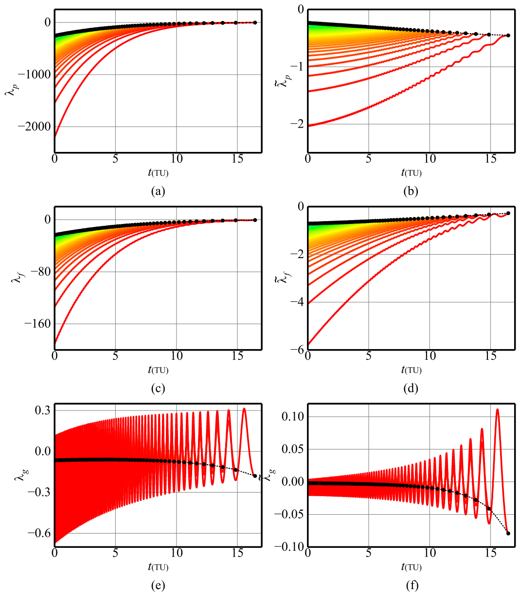
The costate histories presented in Figure 5 further demonstrate the benefit of the scaled formulation. As the continuation proceeds toward higher-energy terminal orbits, the original costates associated with the orbital elements, especially λ p , λ f , and λ g , exhibit a rapid growth in their initial values, consistent with the strong increase in a f and p f . In the last several continuation steps, the differences between neighboring unscaled costates become particularly pronounced, leading to large magnitude separation across the family and making warm-start continuation increasingly difficult. By contrast, after the scaling transformation is introduced, λ ˜ p , λ ˜ f , and λ ˜ g remain well confined within the same order of magnitude throughout the branch, indicating that the dominant growth trend has been effectively absorbed by the scaling. This significantly improves the numerical similarity between adjacent solutions and is particularly important near the pre-escape regime, where the continuation would otherwise become much harder to maintain.
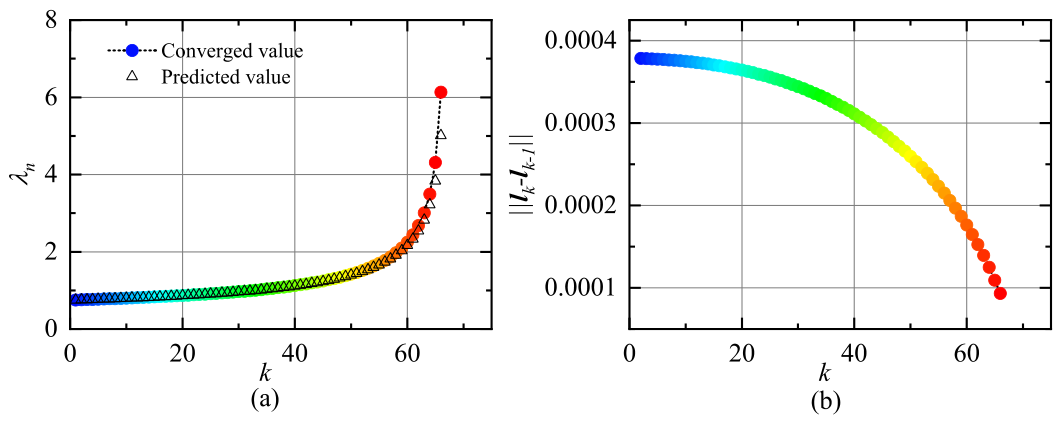
A more quantitative view of this regularity is given in Figure 6. The left panel shows the converged values of the costate magnitude λ n together with the predicted values for the next continuation step. The two sets of points almost overlap over the entire continuation range, indicating that λ n evolves in a highly structured manner and can be extrapolated accurately from the previous solution. This directly validates the predictor introduced in Equation (21). The right panel reports the Euclidean variation in the normalized direction vector, which remains small and changes smoothly during continuation. Therefore, the dominant evolution of the initial costate occurs in its magnitude rather than in its direction. In practical terms, this means that the previous converged direction l k already provides an excellent initial guess for the next step, while only a mild correction of λ n is required. This property is particularly favorable for many-revolution indirect shooting, because it explains why the continuation branch can be advanced reliably over a wide range before entering the near-escape region.
Figure 5. Histories of the original and scaled costates for all continuation solutions. The color varies from cold to warm, corresponding to the continuation results from steps 1 to 66. The black dots denote the terminal values of the corresponding costate history at each continuation step. Histories of the original and scaled costates for all continuation solutions: (a) λ p ; (b) λ ˜ p ; (c) λ f ; (d) λ ˜ f ; (e) λ g ; and (f) λ ˜ g . The color varies from cold to warm, corresponding to the continuation results from steps 1 to 66, and the color assigned to each solution is consistent with that of the corresponding continuation step k in Figure 5 and Figure 7. The black dots denote the terminal values of the corresponding costate history at each continuation step.
Aerospace 13 00429 g005
Figure 6. (a) The corresponding magnitude λ n along the continuation steps. (b) Variation in the Euclidean distance between neighboring normalized costate directions.
Aerospace 13 00429 g006
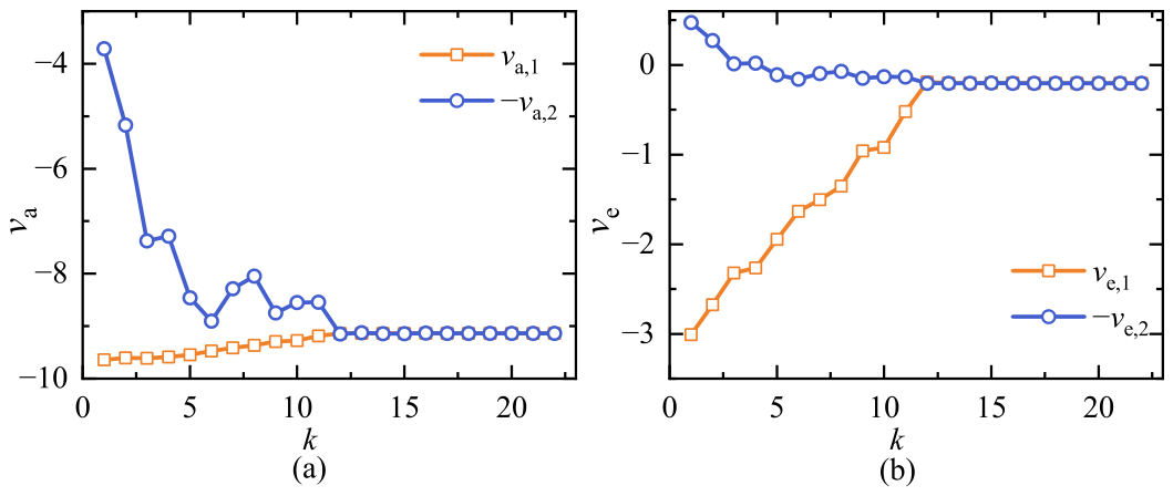
Figure 7. Iteration histories of the Lagrange multipliers associated with the interface constraints: (a) Lagrange multiplier for the semi-major axis constraint; (b) Lagrange multiplier for the eccentricity constraint.
Aerospace 13 00429 g007

5.2. Outer-Level Iteration Optimization Results

Since both the forward GTO-raising subproblem and the backward DRO insertion subproblem can be solved with robust convergence properties, the corresponding Lagrange multipliers associated with the intermediate-interface constraints can be obtained reliably. Based on these multipliers, the interface variables ( a * , e * ) are further corrected in an outer-level differential-correction procedure to enforce the stationarity condition of the overall problem. Specifically, the Jacobian matrix with respect to ( a * , e * ) is evaluated by finite differences, where the perturbation steps are chosen as δ a = 0.0001 and δ e = 0.0001 . The resulting sensitivity information is then used to iteratively update ( a * , e * ) until the interface matching condition error F is less than ε = 10 4 .
Figure 7 compares the evolution of the Lagrange multipliers associated with the interface constraints, which represent the sensitivities of the total cost with respect to the interface parameters in the two phases. For clarity, the multipliers of the second phase are plotted with a reversed sign, so that coincidence of the two curves directly indicates sensitivity balance at the interface. Both the semi-major axis and eccentricity constraint sensitivities converge to a common value, with the former reaching 9.1375 and the latter 0.2034 . This means that, at convergence, the forward and backward phases have equal first-order sensitivities with respect to both interface parameters, and therefore small perturbations of a * or e * no longer produce a first-order change in the total cost T sum . The convergence histories also indicate that the second phase is more sensitive to the semi-major axis, while the first phase is more sensitive to the eccentricity.
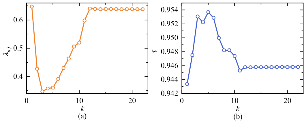
Figure 8 shows the evolution of the shooting variables λ n , 0 and τ . Both variables remain in a narrow range throughout the iteration and converge to stable values, with λ n , 0 = 0.6380 and τ = 0.9458 . The converged phase indicates that the optimal insertion point is close to, but not exactly at the far-Earth-side reference point τ = 1 . The convergence performance is shown in Figure 9. The residual norm F decreases rapidly and becomes nearly zero after about twelve iterations, indicating that the interface mismatch has been effectively removed. At the same time, the total flight time decreases monotonically toward a stable minimum. The converged total flight time is 19.3609 TU , with T 1 = 16.3807 TU and T 2 = 2.9802 TU . This confirms that the outer-level iteration not only enforces interface consistency, but also drives the composite transfer toward a locally optimal time performance.
The local optimality of the converged interface parameters is further verified by the contour maps in Figure 10 and Figure 11. In both cases, the marked point at a = 0.470125 and e = 0.247914 is located at the same local optimum region. This demonstrates that minimizing the multiplier mismatch is fully consistent with minimizing the total flight time in the ( a , e ) plane. The contour patterns also show a steeper variation in the a-direction than in the e-direction, which is consistent with the larger magnitude of the converged a-sensitivity observed in Figure 7.
These results confirm that the proposed outer-level interface optimization can identify an interface orbit for which the two locally optimal phases are first-order matched and the total transfer time is locally minimized. More importantly, the converged values of a * , e * , λ n , 0 , and τ provide a numerically precise and dynamically consistent initial guess for the subsequent fully coupled optimization problem.

5.3. Fully Coupled Time-Optimal Solution

After the bidirectional initialization and the interface correction procedure, the fully coupled 13-variable shooting problem converges to a continuous time-optimal transfer from the GTO departure orbit to the target DRO. The resulting trajectory is shown in Figure 12 in both the Earth-centered inertial frame and the Earth–Moon rotating frame. In Figure 12a, the black solid curve represents the target 2:1 DRO baseline. Its ellipse-like appearance in the inertial frame reflects the fact that the 2:1 DRO period is one-half of the lunar orbital period; consequently, within one revolution of the dashed lunar reference orbit, the DRO completes two far-side-to-near-side-to-far-side passages. In contrast, in Figure 12b, the same DRO baseline appears as a closed curve around the Moon, with a visibly wider extent in the y-direction, which more directly reflects its local synodic-frame geometry near the Moon.
The blue trajectory in both panels denotes the GTO-raising phase. In the inertial frame, its revolution-by-revolution outward expansion clearly shows the gradual growth of the Earth-centered orbit before reaching the intermediate interface. The red trajectory denotes the DRO insertion phase. In Figure 12a, this segment starts from the intermediate interface and departs smoothly from the end of the GTO-raising arc without any visible corner or break, which is a necessary geometric feature of a continuous two-phase solution. The same red arc then approaches the target DRO smoothly and becomes tangent to the DRO baseline before entering it at the marked insertion point. In Figure 12b, the interface point again represents the same physical connection between the two phases, but now expressed in the rotating frame, where the red segment can be interpreted more clearly as the lunar-approach and terminal capture process. Therefore, the two panels together show that the interface is not merely an auxiliary matching point, but the common physical connection at which the Earth-centered spiral-out phase transitions continuously into the DRO insertion phase.
This geometric interpretation is also consistent with the coupled interface conditions introduced in Section 4.2, where the two phase solutions are matched through the common interface quantities ( a , e , m , Δ ϕ ) . In particular, the smooth connection seen in Figure 12 is further supported by the continuity histories in Figure 13. In addition, the optimized insertion phase is τ f = 0.94634 , which indicates that the final insertion point lies very close to the far-Earth-side reference phase τ = 1 , but slightly in advance of it. This is physically reasonable for the minimum-time problem, since an earlier phase entry can reduce the total transfer time while still allowing a smooth terminal capture onto the target DRO.
Figure 13 further examines the evolution of the interface constrained state variables along the complete transfer. All state variables are smoothly connected at the intermediate interface. The semi-major axis increases in a regular manner during the GTO-raising phase, which indicates a monotonic energy growth of the Earth-centered orbit. Meanwhile, the eccentricity decreases in an overall regular fashion, showing the gradual circularization tendency of the low-thrust raising process. The mass decreases continuously and almost linearly, since the thrust remains saturated throughout the transfer. During the GTO-raising phase, Δ ϕ exhibits a variation pattern similar to the orbital period due to the multi-revolution process; this periodic behavior vanishes once the spacecraft approaches the lunar vicinity. These trends are consistent with the thrust history in Figure 14, where the first-phase thrust direction is primarily aligned with the tangential direction and therefore mainly acts to increase the orbital energy. After the interface point, however, the variations in a and e no longer follow the same regular pattern. This change is physically expected, because once the spacecraft enters the lunar vicinity, the Moon’s gravity becomes significant and the transfer dynamics can no longer be interpreted as a simple Earth-centered low-thrust orbit-raising process. In particular, the mass and the relative phase angle Δ ϕ coincide exactly at the connection point. This is essential for the physical validity of the final transfer, because without simultaneous continuity of m and Δ ϕ , the two locally optimal phases would not represent a realizable continuous trajectory under the fully coupled model.
The control profiles of the two phases are presented in Figure 14. For the first phase, the thrust direction in the local orbital frame is dominated by the tangential component u t , while the radial component u r mainly oscillates with the orbital phase. This is consistent with the role of the first phase, namely, to raise the orbital energy efficiently during the long GTO-raising process. By contrast, the control history of the DRO insertion phase, expressed in the rotating-frame components ( u x , u y ) , is determined by the coupled state–costate evolution near the Moon. Its structure is therefore less intuitive from a purely geometric viewpoint, which also reflects the stronger dynamical coupling in the terminal insertion stage.
To quantify the quality of the initialization more explicitly, Table 3 and Table 4 now report not only the absolute difference but also the relative error of each shooting variable with respect to the final optimized value. For the first phase, most variables remain close to their converged values. The largest relative error in Table 3 is 72.31 % for l L , 0 , followed by 66.67 % for l g , 0 . These two relatively large percentages are associated with variables whose optimal values are very close to zero, so even a very small absolute deviation leads to a comparatively large relative error. For the remaining first-phase variables, the relative errors remain moderate, for example 15.84 % for λ n , 0 and 2.95 % for ϕ 0 , which indicates that the first-phase initialization still stays close to the final optimized solution overall.
For the second phase, the agreement between the bidirectional initial guess and the converged solution is also good. The largest relative error in Table 4 is 11.75 % for λ v x , f , while the other terminal costate components remain within 2.26 % . The terminal mass m f and the DRO phase parameter τ f show particularly small deviations, with relative errors of only 0.0046 % and 0.0539 % , respectively. Overall, these results indicate that the proposed bidirectional initialization provides a sufficiently accurate starting point for the fully coupled indirect shooting problem and places both phases in the neighborhood of the final converged optimum.
These results indicate that the proposed initialization places both segmental subproblems directly in the neighborhood of the final optimum. The particularly high accuracy of the first phase initialization is physically reasonable, because before reaching the interface the trajectory is still mainly governed by the Earth’s gravity, and the lunar perturbation remains relatively weak. As a result, the forward phase is less sensitive to the full three-body dynamic coupling, so the inferred initial shooting variables stay very close to those of the final optimized solution. As a result, the 13-dimensional nonlinear indirect optimal control problem becomes numerically tractable and converges rapidly to the mathematically optimal solution, which confirms the effectiveness of the proposed framework.

5.4. Robustness Assessment of the Initialization

The robustness of the proposed initialization is further assessed by Monte Carlo random-shooting tests. For the present GTO-to-DRO transfer, a conventional direct end-to-end transcription is difficult to apply directly because the long multi-revolution GTO-raising phase would require an excessively large number of mesh points. A conventional indirect shooting formulation is also impractical without a high-quality initial guess, since its convergence basin is extremely narrow and arbitrary costate guesses usually fail to generate a valid terminal event. Moreover, existing indirect initialization strategies based on analytical costate estimation are not directly applicable to the present multi-phase problem with a free DRO phase, interface constraints, and heterogeneous dynamical models [19]. Therefore, to provide a meaningful comparison and to quantify the convergence robustness of the shooting problems, controlled random perturbations are generated around the converged reference solutions. This Monte Carlo assessment evaluates the local attraction basin of each stage and demonstrates whether the proposed initialization can provide reliable starting values for the complete indirect optimization.
For the forward GTO-raising phase, the scaled initial costate is expressed by its direction and magnitude, as introduced in Equation (A6). This parameterization allows the directional and magnitude errors in the initial costate guess to be examined separately. Table 5 compares the initial costate parameters obtained from the maximum-energy strategy with those of the fixed- ( a * , e * ) optimum, where a * = 0.47013 and e * = 0.24791 are prescribed interface parameters for this local GTO-raising subproblem. It should be noted that this fixed- ( a * , e * ) optimum is used as the reference solution for the present robustness assessment, and is different from the first-phase optimum reported in Section 5.3, where the interface parameters have already been corrected by the outer-level iteration and further refined in the fully coupled problem.
As shown in Table 5, the maximum-energy strategy provides a costate direction close to that of the fixed- ( a * , e * ) optimum, whereas the magnitude parameter λ n , 0 differs substantially. This indicates that the maximum-energy continuation mainly captures the directional structure required by the subsequent fixed- ( a * , e * ) time-optimal shooting problem, while the costate magnitude still needs to be corrected during the shooting iteration. Therefore, the directional and magnitude sensitivities are examined separately.
For the direction-perturbation test, the magnitude λ n , 0 is fixed at its optimal value, while each component of the optimal costate-direction vector is perturbed by a prescribed relative level ρ . The perturbed initial guess for the j-th random trial is generated as
l 0 ( j ) = l 0 * + ρ ξ ( j ) l 0 * , λ n , 0 ( j ) = λ n , 0 * ,
Here, j denotes the random-trial index, ξ ( j ) is a random vector with components uniformly distributed in [ 1 , 1 ] , ∘ denotes the component-wise product, and ρ is the prescribed relative perturbation level. For each value of ρ , 50 independent random trials are performed.
The results are shown in Table 6. The forward shooting problem remains fully convergent for direction perturbations of 0.5 % and 1 % . When the perturbation level increases to 5 % , the success rate decreases to 58 % , and it further drops to 12 % at 10 % . This behavior confirms that the fixed- ( a , e ) GTO-raising TPBVP is primarily sensitive to the costate direction. Once the direction is not sufficiently accurate, the propagated trajectory may fail to reach the expected apogee terminal event, so the shooting residual cannot be reduced effectively. The function evaluations and CPU time also increase with the perturbation level, indicating that larger direction errors require a more difficult nonlinear correction even for successful trials.
For the magnitude-scaling test, the optimal direction is fixed and only the costate magnitude is changed as
l 0 ( j ) = l 0 * , λ n , 0 ( j ) = k λ n , 0 * ,
where k is the prescribed scale factor. This test is closely related to the homogeneous structure of the Hamiltonian system with respect to the costate variables. In particular, a uniform scaling of the costate vector does not change the normalized costate direction, and the optimal thrust direction in Equation (9) is mainly determined by this direction rather than by the absolute magnitude of the costates. Therefore, once the costate direction is sufficiently close to that of the optimal solution, the magnitude error can be corrected separately during the nonlinear shooting iteration.
As shown in Table 7, all non-nominal scale factors converge to the reference solution, even when the costate is changed by two orders of magnitude. This confirms that the convergence of the GTO-raising shooting problem is much less sensitive to the magnitude than to the direction of the initial costate. Nevertheless, very large scale factors still increase the function evaluations and CPU time, indicating that the magnitude affects the conditioning and efficiency of the nonlinear correction. This result also explains why the maximum-energy strategy is effective for the subsequent fixed- ( a , e ) problem: although its costate magnitude may differ considerably from the fixed- ( a , e ) optimum, it already provides a costate direction close to the optimal one, which is the key factor for entering the correct convergence basin.
The same type of local robustness test is then applied to the backward DRO-insertion subproblem. The shooting vector s back in Equation (64) is perturbed around the converged reference solution by
s back ( j ) = s back * + ρ ξ ( j ) s back * ,
where each perturbation level again contains 50 independent random trials. The results in Table 8 show that the backward shooting problem is also sensitive to the initial adjoint variables. The success rate remains 86 % for a 1 % perturbation, but decreases to 14 % and 8 % for 10 % and 20 % perturbations, respectively. This means that the pseudospectral solution and covector mapping do not need to provide an extremely accurate costate estimate, but they must still place the backward shooting variables within a reasonably close neighborhood of the optimal solution.
Finally, the complete 13-dimensional shooting vector in Equation (108) is perturbed around the fully coupled optimal solution. Each perturbation level contains 50 independent trials. The results are summarized in Table 9. Compared with the two segmental subproblems, the full GTO-to-DRO shooting problem has a much narrower convergence basin. A 0.5 % perturbation already reduces the success rate to 60 % , and a 5 % perturbation leads to only 6 % successful convergence. This sharp reduction is expected because the full problem simultaneously contains the forward costate direction, the costate magnitude, the lunar phase, the backward terminal costates, the terminal mass, and the DRO phase parameter. Small inconsistencies among these variables can destroy the interface matching and the terminal transversality conditions at the same time.
It should be emphasized that the above robustness tests are not intended to provide a global convergence guarantee for arbitrary perturbations. The perturbations are imposed as component-wise uniform relative errors around the reference solution. In the actual indirect shooting problem, however, the convergence basin may be highly anisotropic: some costate components or parameter directions can be extremely sensitive, whereas others may have only a weak influence on convergence. In addition, when some reference components are close to zero, their relative perturbations may have limited physical meaning. Therefore, failure or success outside the tested perturbation ranges should not be interpreted as a strict boundary of the true convergence domain. Rather, these Monte Carlo tests provide a practical local assessment of how rapidly the convergence deteriorates when the initial guess departs from the optimal neighborhood.
Within this interpretation, the perturbation results clearly show that even guesses generated around the optimal solution must remain within a sufficiently small neighborhood to ensure reliable convergence. This also implies that completely unstructured random guesses, which have no information about the costate direction, terminal phase, or interface consistency, are highly unlikely to converge for the present multi-phase TPBVP. Therefore, the proposed initialization is not merely a numerical convenience, but a necessary mechanism for making the complete indirect shooting problem tractable. For the GTO-raising phase, the maximum-energy continuation provides a costate direction that is already close to that of the fixed- ( a , e ) optimum, while the remaining magnitude mismatch can be corrected by the shooting iteration. For the DRO-insertion phase, the pseudospectral solution and covector mapping provide a sufficiently close estimate of the terminal costates. After the interface stationarity correction and lunar-phase matching, these two guided guesses form a complete 13-variable initial vector located inside the narrow convergence basin of the fully coupled TPBVP. Therefore, the proposed bidirectional initialization framework provides a practical route for solving the time-optimal low-thrust GTO-to-DRO transfer, whereas arbitrary indirect guesses would almost certainly fail for this highly sensitive multi-phase problem.


6. Conclusions

This paper addressed the overall time-optimal low-thrust GTO-to-DRO transfer problem, which is difficult to solve satisfactorily by either direct or indirect methods alone. For such long-duration multi-phase transfers, direct methods suffer from the rapid growth of discretization nodes and computational burden under multi-revolution orbit raising and precise terminal insertion in a multi-body dynamical environment, while indirect methods remain highly sensitive to the initial guesses of the state, costate, and phase variables and are therefore difficult to converge without a reliable initialization strategy.
To overcome these difficulties, a bidirectional initialization framework was developed by combining a forward initialization for the multi-revolution GTO-raising phase, a backward initialization for the DRO-insertion phase, and an outer-level interface-matching iteration. Based on this construction, the full problem was further refined as a fully coupled indirect shooting problem with lunar phase continuity and lunar perturbations restored.
The results showed that the proposed framework can provide a reliable and physically consistent initial guess for the complete optimization problem, and that the initialized variables remain very close to the final optimal solution. This indicates that the proposed bidirectional construction can capture the essential state–costate structure of the overall time-optimal transfer and substantially improve the solvability of a class of problems that are otherwise difficult for either direct or indirect methods used alone. Therefore, this method may also serve as a useful reference for future extensions to higher-fidelity cislunar models and other long-duration multi-phase low-thrust transfer problems.

Author Contributions

Conceptualization, C.Q. and N.Z.; methodology, C.Q.; software, C.Q.; validation, C.Q. and N.Z.; formal analysis, C.Q. and N.Z.; investigation, C.Q. and N.Z.; resources, C.Q. and N.Z.; data curation, C.Q. and N.Z.; writing—original draft preparation, C.Q.; writing—review and editing, C.Q.; visualization, C.Q.; supervision, C.Q. and S.S.; project administration, C.Q. and S.S.; funding acquisition, W.M. and H.C.; All authors have read and agreed to the published version of the manuscript.

Funding

This work is supported by Shanghai Aerospace Science and Technology Innovation Fund (No. SAST2024-034) and the National Natural Science Foundation of China (No. U20B2001).

Data Availability Statement

The original contributions presented in this study are included in the article. Further inquiries can be directed to the corresponding author.

Conflicts of Interest

The authors declare no conflicts of interest.

Appendix A. Costate Scaling and Initial Costate Parameterization

This appendix provides the detailed expressions for the costate scaling and the initial-costate parameterization used in the forward shooting formulation. These relations are needed to construct the scaled costate variables, define the shooting unknowns, and support the continuation procedure described in Section 2.1.
Starting from the scaling definition in Equation (11), the inverse transformation is
λ p = λ ˜ p p 2 , λ f = λ ˜ f p , λ g = λ ˜ g p ,
and the scaled costate dynamics follow from the chain rule as
λ ˜ ˙ p = p 2 λ ˙ p + 2 p p ˙ λ p , λ ˜ ˙ f = p λ ˙ f + p ˙ λ f , λ ˜ ˙ g = p λ ˙ g + p ˙ λ g .
For the shooting initialization, the scaled initial costate is expressed in terms of its overall magnitude and direction. Let the scaled costate vector be
λ ˜ = λ ˜ p λ ˜ f λ ˜ g λ L λ m T ,
with norm
λ n = λ ˜ ,
and unit direction
l = λ ˜ λ n , l R 5 , l = 1 .
The initial scaled costate can therefore be written as
λ ˜ = λ n l .
This decomposition separates the slowly varying directional information from the overall scale variation along the continuation family, which is why it is effective for warm-starting the indirect shooting iterations from one continuation step to the next.

Appendix B. The Null-Space Operator

For a matrix G R n × m , the null-space operator null ( G T ) denotes a matrix whose columns form a basis of the null space of G T , namely,
N ( G T ) = z R n : G T z = 0 .
Accordingly, if
N = null G T ,
then every column of N satisfies
G T N = 0 .
If rank ( G ) = r , then by the rank–nullity theorem the dimension of N ( G T ) is
dim N ( G T ) = n r ,
so that the null-space basis matrix has size
N R n × ( n r ) .
A standard way to compute N is through the singular value decomposition
G T = U Σ V T .
If V is partitioned as
V = V r V 0 ,
where V 0 contains the right singular vectors associated with the zero singular values, then
N = V 0 .
Therefore, null ( G T ) returns an orthonormal basis of all vectors orthogonal to the column space of G .

Appendix C. Jacobian Matrix of G2

For the DRO insertion phase, the Jacobian matrix of the intermediate-point constraints with respect to the state vector
X = x y v x v y m T
is written as
G 2 = a X e X Γ X m X T .
For compactness, introduce
ρ = ( x + μ ) 2 + y 2 , D = ( v x y ) 2 + ( v y + x + μ ) 2 2 ( 1 μ ) ρ ,
and
h = ( x + μ ) ( v y + x + μ ) y ( v x y ) .
The partial derivative of the semi-major axis constraint with respect to the state vector is
a X = 1 μ D 2 2 ( v y + x + μ ) + 2 ( 1 μ ) ( x + μ ) ρ 3 2 ( v x y ) + 2 ( 1 μ ) y ρ 3 2 ( v x y ) 2 ( v y + x + μ ) 0 T .
The partial derivative of the eccentricity constraint with respect to the state vector is
e X = 1 2 e ( 1 μ ) 2 h 2 2 ( v y + x + μ ) + 2 ( 1 μ ) ( x + μ ) ρ 3 + 2 D h v y + 2 ( x + μ ) h 2 2 ( v x y ) + 2 ( 1 μ ) y ρ 3 + 2 D h v x + 2 y 2 h 2 ( v x y ) 2 D h y 2 h 2 ( v y + x + μ ) + 2 D h ( x + μ ) 0 T .
The partial derivative of the apse-section event function with respect to the state vector is
Γ X = v x v y x + μ y 0 .
The partial derivative of the mass constraint with respect to the state vector is
m X = 0 0 0 0 1 .

References

  1. Wang, M.; Zhang, C.; Zhang, H. Mechanism analysis of the DRO low-energy transfer problem: An energy perspective. Astrodynamics 2025, 9, 165–193. [Google Scholar] [CrossRef] [Scilit]
  2. Pozzi, C.; Pontani, M.; Beolchi, A.; Fantino, E. Optimal low-thrust orbit transfers connecting Gateway with Earth and Moon. Acta Astronaut. 2025, 228, 1107–1121. [Google Scholar] [CrossRef] [Scilit]
  3. Peng, C.; Shang, Y.; He, S.; Zhu, Z.; Wen, C. Low-energy transfers to lunar distant retrograde orbits from geostationary transfer orbits. J. Spacecr. Rocket. 2024, 61, 1293–1304. [Google Scholar] [CrossRef] [Scilit]
  4. Zhang, J.; Yu, H.; Dai, H. Overview of Earth-Moon Transfer Trajectory Modeling and Design. Comput. Model. Eng. Sci. (CMES) 2023, 135, 5–43. [Google Scholar] [CrossRef] [Scilit]
  5. Shannon, J.L.; Ozimek, M.T.; Atchison, J.A.; Hartzell, C.M. Rapid design of high-fidelity low-thrust transfers to the moon. J. Spacecr. Rocket. 2022, 59, 1522–1535. [Google Scholar] [CrossRef] [Scilit]
  6. Malyuta, D.; Yu, Y.; Elango, P.; Açıkmeşe, B. Advances in trajectory optimization for space vehicle control. Annu. Rev. Control 2021, 52, 282–315. [Google Scholar] [CrossRef] [Scilit]
  7. Betts, J.T.; Erb, S.O. Optimal low thrust trajectories to the moon. SIAM J. Appl. Dyn. Syst. 2003, 2, 144–170. [Google Scholar] [CrossRef] [Scilit]
  8. Fan, Z.; Huo, M.; Qi, J.; Qi, N. Fast initial design of low-thrust multiple gravity-assist three-dimensional trajectories based on the Bezier shape-based method. Acta Astronaut. 2021, 178, 233–240. [Google Scholar] [CrossRef] [Scilit]
  9. Vijayakumar, M.; Abdelkhalik, O. Shape-based approach for low-thrust earth–moon trajectories initial design. J. Guid. Control Dyn. 2022, 45, 103–120. [Google Scholar] [CrossRef] [Scilit] [PubMed]
  10. Li, J.; Zhang, G.; Cui, L. A Fast Midcourse Trajectory Optimization Method for Interceptors Based on the Bézier Curve. Aerospace 2025, 12, 893. [Google Scholar] [CrossRef] [Scilit]
  11. Oshima, K. Regularized direct method for low–thrust trajectory optimization: Minimum–fuel transfer between cislunar periodic orbits. Adv. Space Res. 2023, 72, 2051–2063. [Google Scholar] [CrossRef] [Scilit]
  12. Hofmann, C.; Topputo, F. Homotopic Approach for High-Fidelity Convex Low-Thrust Trajectory Optimization. IEEE Trans. Aerosp. Electron. Syst. 2025, 61, 11991–12007. [Google Scholar] [CrossRef] [Scilit]
  13. Jiang, F.; Baoyin, H.; Li, J. Practical techniques for low-thrust trajectory optimization with homotopic approach. J. Guid. Control Dyn. 2012, 35, 245–258. [Google Scholar] [CrossRef] [Scilit]
  14. Hu, J.; Yang, H.; Li, S.; Liang, G. Rapid trajectory design for low-thrust many-revolution rendezvous using analytical derivations. J. Guid. Control Dyn. 2025, 48, 1449–1457. [Google Scholar] [CrossRef] [Scilit]
  15. Zhang, C.; Topputo, F.; Bernelli-Zazzera, F.; Zhao, Y.S. Low-thrust minimum-fuel optimization in the circular restricted three-body problem. J. Guid. Control Dyn. 2015, 38, 1501–1510. [Google Scholar] [CrossRef] [Scilit]
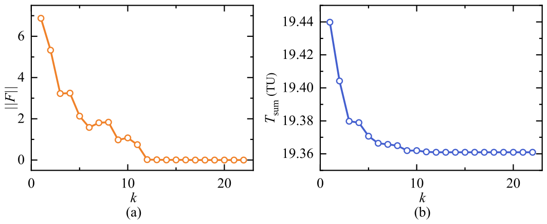
  16. Lee, D.; Bang, H.; Kim, H.D. Optimal earth-moon trajectory design using new initial costate estimation method. J. Guid. Control Dyn. 2012, 35, 1671–1676. [Google Scholar] [CrossRef] [Scilit]
  17. Ayyanathan, P.J.; Taheri, E. Mapped adjoint control transformation method for low-thrust trajectory design. Acta Astronaut. 2022, 193, 418–431. [Google Scholar] [CrossRef] [Scilit]
  18. Wu, D.; Wang, W.; Jiang, F.; Li, J. Minimum-time low-thrust many-revolution geocentric trajectories with analytical costates initialization. Aerosp. Sci. Technol. 2021, 119, 107146. [Google Scholar] [CrossRef] [Scilit]
  19. Wu, D.; Cheng, L.; Jiang, F.; Li, J. Analytical costate estimation by a reference trajectory-based least-squares method. J. Guid. Control Dyn. 2022, 45, 1529–1537. [Google Scholar] [CrossRef] [Scilit]
  20. Chen, S.; Li, H.; Baoyin, H. Multi-rendezvous low-thrust trajectory optimization using costate transforming and homotopic approach. Astrophys. Space Sci. 2018, 363, 128. [Google Scholar] [CrossRef] [Scilit]
  21. Yoon, S.W.; Petukhov, V.; Ivanyukhin, A. An approach for end-to-end optimization of low-thrust interplanetary trajectories using collinear libration points. Acta Astronaut. 2024, 221, 12–25. [Google Scholar] [CrossRef] [Scilit]
  22. Yin, Q.; Wu, G.; Sun, G.; Gu, Y. Multi-objective orbital maneuver optimization of multi-satellite using an adaptive feedback learning NSGA-II. Swarm Evol. Comput. 2025, 93, 101835. [Google Scholar] [CrossRef] [Scilit]
  23. Gu, Y.; Liu, H.; Pan, T.; Bai, S.; Liu, J.; Wu, Y.; Wu, G. Ensemble time freedom heuristic and intelligent optimization algorithm for relay satellites scheduling considering multi-type task requirements. Expert Syst. Appl. 2026, 316, 131815. [Google Scholar] [CrossRef] [Scilit]
  24. Du, C.; Song, L.; Zhang, J.; Liu, Y. A novel calculation method for low-thrust transfer trajectories in the Earth-Moon restricted three-body problem. Aerosp. Sci. Technol. 2024, 147, 109048. [Google Scholar] [CrossRef] [Scilit]
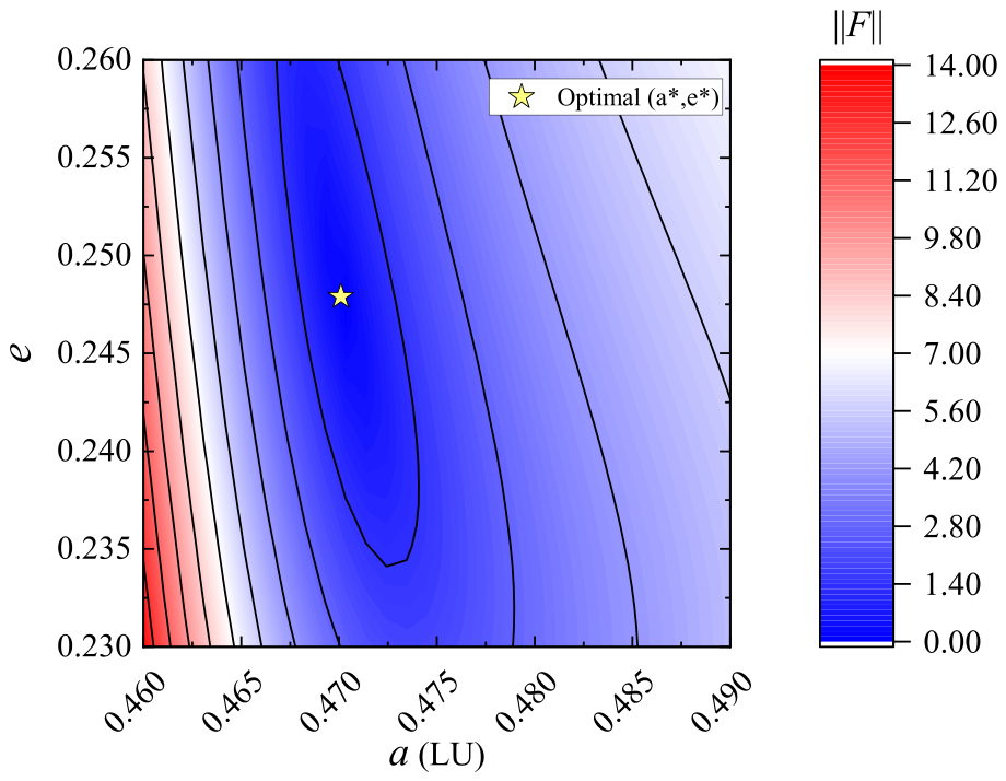
  25. Sidhoum, Y.; Oguri, K. Indirect forward–backward shooting for low-thrust trajectory optimization in complex dynamics. J. Guid. Control Dyn. 2024, 47, 2164–2172. [Google Scholar] [CrossRef] [Scilit]
  26. Alvarado, K.I.; Singh, S.K. Exploring the Design Space of Low-Thrust Transfers with Ballistic Terminal Coast Segments in Cis-Lunar Space. Aerospace 2025, 12, 217. [Google Scholar] [CrossRef] [Scilit]
  27. Suslov, K.; Shirobokov, M.; Tselousova, A. Minimum-energy transfer optimization between near-circular orbits using an approximate closed-form solution. Aerospace 2023, 10, 1002. [Google Scholar] [CrossRef] [Scilit]
  28. Quarta, A.A.; Mengali, G. Minimum-time space missions with solar electric propulsion. Aerosp. Sci. Technol. 2011, 15, 381–392. [Google Scholar] [CrossRef] [Scilit]
  29. Chi, Z.; Li, H.; Jiang, F.; Li, J. Power-limited low-thrust trajectory optimization with operation point detection. Astrophys. Space Sci. 2018, 363, 122. [Google Scholar] [CrossRef] [Scilit]
  30. Lin, X.; Zhang, G.; Vazquez, R. Spacecraft Constant-Thrust Minimum-Time Rendezvous via Reachable Set Theory. IEEE Trans. Aerosp. Electron. Syst. 2025, 61, 13224–13232. [Google Scholar] [CrossRef] [Scilit]
  31. Guo, X.; Wu, D.; Jiang, F. Minimum-time rendezvous via simplified initial costate normalization and auxiliary orbital transfer. J. Guid. Control Dyn. 2023, 46, 1627–1636. [Google Scholar] [CrossRef] [Scilit]
  32. Zhao, C.; Liu, A.; Jiang, A.; Zheng, X.; Wang, H.; Zhao, R. Design and Implementation of a Reduced-Space SQP Solver with Column Reordering for Large-Scale Process Optimization. Algorithms 2025, 18, 699. [Google Scholar] [CrossRef] [Scilit]
  33. Wang, M.; Yang, C.; Sun, Y.; Zhang, H. Family of 2:1 resonant quasi-periodic distant retrograde orbits in cislunar space. Front. Astron. Space Sci. 2024, 11, 1352489. [Google Scholar] [CrossRef] [Scilit]
  34. Patterson, M.A.; Rao, A.V. GPOPS-II: A MATLAB software for solving multiple-phase optimal control problems using hp-adaptive Gaussian quadrature collocation methods and sparse nonlinear programming. ACM Trans. Math. Softw. (TOMS) 2014, 41, 1. [Google Scholar] [CrossRef] [Scilit]
  35. Spada, F.; Sagliano, M.; Topputo, F. Direct–indirect hybrid strategy for optimal powered descent and landing. J. Spacecr. Rocket. 2023, 60, 1787–1804. [Google Scholar] [CrossRef] [Scilit]
  36. Benson, D.A.; Huntington, G.T.; Thorvaldsen, T.P.; Rao, A.V. Direct trajectory optimization and costate estimation via an orthogonal collocation method. J. Guid. Control Dyn. 2006, 29, 1435–1440. [Google Scholar] [CrossRef] [Scilit]
  37. Ceccherini, S.; Mani, K.V.; Topputo, F. Combined System–Trajectory Design for Geostationary Orbit Platforms on Hybrid Transfer. J. Spacecr. Rocket. 2022, 59, 448–466. [Google Scholar] [CrossRef] [Scilit]
Figure 1. Forward GTO-raising phase and backward DRO insertion phase in the Earth-centered inertial frame. Schematic of forward GTO-raising phase and backward DRO insertion phase in the Earth-centered inertial frame. The dark-blue trajectories denote the forward GTO-raising solutions of the maximum-energy problem with different terminal longitudes L f ( k ) , marked by the yellow triangles. The light-blue trajectory denotes the backward DRO insertion phase in the inertial frame. The green triangle indicates the intermediate interface, i.e., the tangency point on the target-parameter orbit. The red and yellow curves represent the reference DRO and the Moon orbit, respectively, and the star marks the DRO insertion point. The purple circle marks the GTO perigee departure point. The forward phase spacecraft–Moon angle Δ ϕ 1 is also indicated. The orange vector illustrates the thrust direction u and its radial and transverse components u r and u t .
Aerospace 13 00429 g001
Figure 2. Intermediate interface and target DRO in the Earth–Moon synodic frame.Schematic of the intermediate interface and the target DRO in the Earth–Moon synodic frame centered at the Earth–Moon barycenter. The dark-blue and light-blue trajectories denote the forward GTO-raising phase and the backward DRO insertion phase, respectively. The green triangle indicates the intermediate interface between the two phases. The spacecraft–Earth and spacecraft–Moon distances are denoted by r 1 and r 2 , respectively. The spacecraft–Moon angle in the backward phase is denoted by Δ ϕ 2 . The purple star marks the DRO insertion point, and its corresponding periodic phase on the DRO is denoted by τ T D . The orange vectors illustrate the unit thrust vector u and its components u x and u y in the synodic frame.
Aerospace 13 00429 g002
Figure 3. GTO-DRO low-thrust bidirectional initialization framework flowchart.
Aerospace 13 00429 g003
Figure 4. Terminal orbital elements of the maximum-energy continuation branch versus the continuation step k. (a) Variation in a f with the continuation step. (b) Variation in e f with the continuation step. (c) Variation in p f with the continuation step. (d) Variation in r a , f with the continuation step.
Aerospace 13 00429 g004
Figure 8. Iteration histories of the auxiliary shooting variables λ n , f in (a) and τ in (b).
Aerospace 13 00429 g008
Figure 9. Convergence histories of the residual norm in (a) and the total flight time in (b).
Aerospace 13 00429 g009
Figure 10. Contour map of F in the neighborhood of the optimum.
Aerospace 13 00429 g010
Figure 11. Contour map of T sum near the optimum.
Aerospace 13 00429 g011
Figure 12. Fully coupled time-optimal GTO–DRO transfer trajectory. (a) Earth-centered inertial-frame view of the final solution. The GTO-raising arc expands outward from the Earth to the intermediate interface, and the DRO insertion arc then departs smoothly from this interface and joins the target 2:1 DRO near the optimized insertion point. The dashed curve denotes the lunar orbital reference, and the black solid curve denotes the target DRO baseline. (b) Earth–Moon rotating-frame view of the same solution. In this frame, the target 2:1 DRO appears as a closed curve around the Moon, and the geometric transition from the Earth-centered spiral-out phase to the lunar-approach and DRO-insertion phase is shown more directly.
Aerospace 13 00429 g012
Figure 13. Evolution of the interface constrained state variables throughout the transfer. The dashed line corresponds to the intermediate interface time, t I = 16.3708 TU . (a) Semi-major axis a. (b) Eccentricity e. (c) Spacecraft mass m. (d) Relative phase angle Δ ϕ .
Aerospace 13 00429 g013
Figure 14. Control histories of the fully coupled optimal transfer in the local thrust coordinate systems of the two phases. (a) Radial and tangential thrust components ( u r , u t ) during the GTO-raising phase. (b) Rotating frame thrust components ( u x , u y ) during the DRO insertion phase.
Aerospace 13 00429 g014
Table 1. Normalized constants and propulsion parameters used in the numerical simulations.
ParameterValueDescription
μ E 398 , 600.4415 km 3 / s 2 Earth gravitational parameter
μ M 4902.8000 km 3 / s 2 Moon gravitational parameter
LU 384 , 388.174 km Earth–Moon distance
TU 375 , 172.945 s Lunar orbital period in radians
VU 1.024560 km / s Characteristic velocity
η 0.7 Propulsion efficiency
P 0 14 kW Available power
I s p 3100 s Specific impulse
g 0 9.806650 m / s 2 Standard sea-level gravitational acceleration
Table 2. Initial GTO and target DRO parameters.
ParameterValueUnit
[ p 0 , f 0 , g 0 , L 0 ] [ 0.030390 , 0.723459 , 0 , 0 ] LU, –, –, rad
m 0 1500kg
[ r p , 0 , r a , 0 ] [ 6777.861 , 42 , 240.950 ] km, km
[ x D , y D , v x , D , v y , D ] | τ = 0 [ 1.175408 , 0 , 0 , 0.494260 ] LU, LU, VU, VU
Table 3. Comparison between the bidirectional initial guess and the final optimized solution for the first-phase shooting variables.
ParameterInitialOptimalAbsolute DifferenceRelative Error (%)
l p , 0 0.36280 0.36751 0.00471 1.28
l f , 0 0.93175 0.92993 0.00182 0.20
l g , 0 0.00005 0.00003 0.00002 66.67
l L , 0 0.00112 0.00065 0.00047 72.31
l m , 0 0.01475 0.01268 0.00207 16.32
λ n , 0 0.63804 0.55078 0.08726 15.84
ϕ 0 ( rad ) 2.28749 2.35705 0.06956 2.95
Table 4. Comparison between the bidirectional initial guess and the final optimized solution for the second-phase shooting variables.
ParameterInitialOptimalAbsolute DifferenceRelative Error (%)
λ x , f 6.13457 5.99875 0.13583 2.26
λ y , f 3.25138 3.21607 0.03531 1.10
λ v x , f 0.15901 0.18019 0.02118 11.75
λ v y , f 5.79937 5.69858 0.10079 1.77
m f ( kg ) 1345.95 1346.01 0.06153 0.0046
τ f 0.94583 0.94634 0.00051 0.0539
Table 5. Comparison between the maximum-energy strategy and the fixed- ( a * , e * ) optimum for the forward GTO-raising shooting variables, with a * = 0.47013 and e * = 0.24791 .
ParameterMaximum-Energy StrategyFixed- ( a , e ) OptimumAbsolute Difference
l p , 0 0.33131 0.36280 0.03149
l f , 0 0.94351 0.93175 0.01176
l g , 0 0.00057 0.00005 0.00061
l L , 0 0.00375 0.00112 0.00263
l m , 0 0.00360 0.01475 0.01114
λ n , 0 6.13556 0.63803 5.49753
Table 6. Random direction perturbation results for the GTO-raising subproblem.
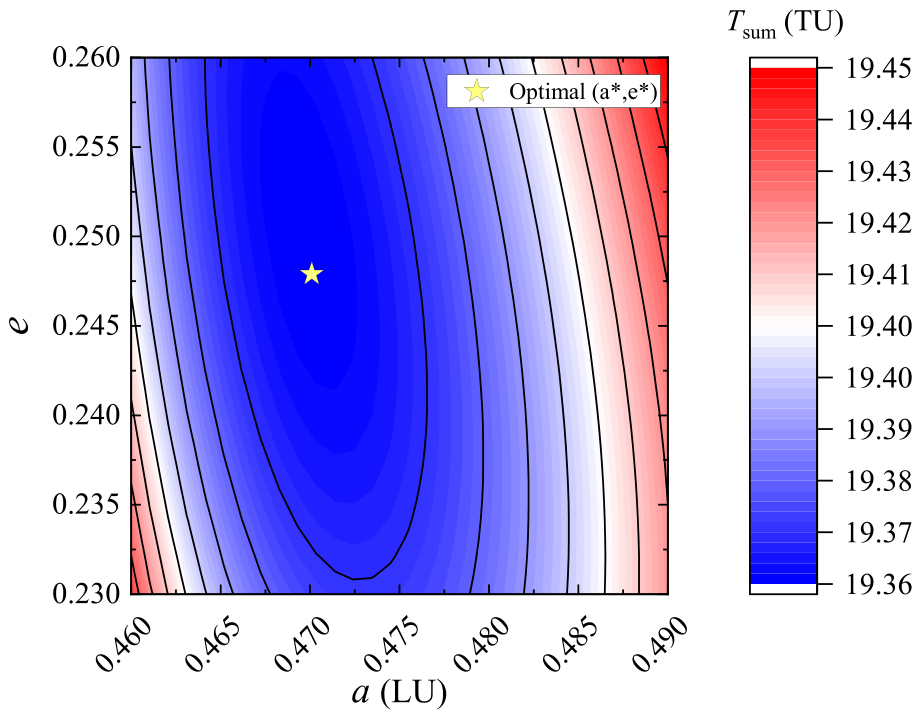
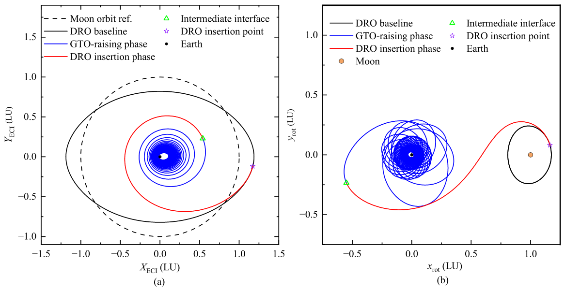
Perturbation LevelSuccess RateAvg. Function Eval. (Successful)Avg. CPU Time (s, Successful)
0.5 % 100 % 35 12.15
1 % 100 % 42 21.15
5 % 58 % 88 43.73
10 % 12 % 156 88.09
Table 7. Magnitude-scaling results for the GTO-raising subproblem with fixed costate direction.
Scale FactorFunction Eval.CPU Time (s)
0.01 28 8.63
0.1 35 10.75
10149 52.42
100520 163.21
Table 8. Random perturbation results for the DRO-insertion subproblem.
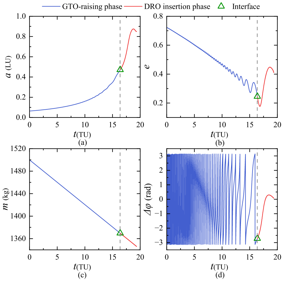
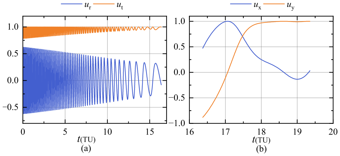
Perturbation LevelSuccess RateAvg. Function Eval. (Successful)Avg. CPU Time (s, Successful)
0.1 % 100 % 45 0.29
1 % 86 % 72 0.44
10 % 14 % 91 0.58
20 % 8 % 146 0.74
Table 9. Random perturbation results for the fully coupled GTO–DRO shooting problem.
Perturbation LevelSuccess RateAvg. Function Eval. (Successful)Avg. CPU Time (s, Successful)
0.1 % 100 % 84 39.71
0.5 % 60 % 112 53.26
1 % 34 % 112 54.12
5 % 6 % 170 75.91
Disclaimer/Publisher’s Note: The statements, opinions and data contained in all publications are solely those of the individual author(s) and contributor(s) and not of MDPI and/or the editor(s). MDPI and/or the editor(s) disclaim responsibility for any injury to people or property resulting from any ideas, methods, instructions or products referred to in the content.