Incremental Nonlinear Reinforcement Learning Control for a Civil Aircraft with Model Uncertainties and Actuator Faults

Abstract

The problem of fault-tolerant attitude tracking control for the civil aircraft with model uncertainties and actuator faults is studied. A robust multiple inversion-based incremental nonlinear dynamic inversion (RMI-INDI) fault-tolerant control method is proposed for the problem. Firstly, considering that the higher-order term is neglected in the INDI method, an RMI method is proposed to deal with the higher-order term and model uncertainties of the INDI control. Secondly, to achieve the optimal control parameters for the INDI controller, a reinforcement learning (RL) method is suggested, where a Deep Deterministic Policy Gradient (DDPG) algorithm with a smooth reward function is designed. Finally, performances of the proposed RL-RMI-INDI fault-tolerant controller are demonstrated by using two scenario simulations. Compared with the SMC control, RMI-NDI control and INDI control without RL, tracking errors and overshoots are greatly reduced by the proposed RL-RMI-INDI controller for attitude tracking missions, even under model uncertainties and actuator faults.

1. Introduction

Flight safety is a hot topic for civil aircraft recently [1]. For instance, many flight accidents result from faults of flight control system, including actuator stuck and sensor failure, etc. These faults not only cause large model uncertainties but also threaten the stability of the system [2]. Therefore, designing a novel fault-tolerant flight control system that maintain aircraft stability under fault conditions and uncertainties becomes a significant challenge for aviation safety.

Due to the strong nonlinear characteristics of the aircraft under actuator faults and model uncertainties, the traditional linear control design at the balance points can hardly meet the control requirements. Feedback linearization (FL) is a kind of important nonlinear control method [3], but this method makes it vulnerable in the presence of model mismatch or unmodeled dynamics. Therefore, researchers have proposed various other methods to enhance robustness, such as H∞ control [4,5,6] and a robust multiple inversion method [7]. To achieve optimal control gain for the robust stabilization system, a differential evolution (DE) algorithms combined with linear matrix inequalities (LMIs) was proposed [8], but the parameters that resulted from DE easily made the system unstable. The Robust Granular Feedback Linearization (RGFL) controller was proposed to combine with Evolutionary Participatory Learning (EPL), which could estimate and compensate model uncertainties online [9,10], but there are no systematic comparisons for measurement noises, model mismatch, and actuator faults. Nonlinear dynamic inversion (NDI) control was achieved by effectively compensating for the nonlinear effects of the system inversion [11,12,13,14]. However, the performances of the NDI controllers were highly dependent on the accuracy of the model [15]. To enhance robustness for model uncertainties, an incremental nonlinear dynamic inversion (INDI) method has been proposed [16,17]. The INDI applies angular acceleration as feedback, which reduces reliance on precise models and overcomes the impact of model uncertainties. Due to its low sensitivity to model parameters, INDI has been successfully applied to many kinds of the aircraft [18,19].

Although INDI reduces the reliance on accurate models and improves robustness by an incremental form, it is a critical issue to maintain performances and to ensure stability of the system with actuator faults. In the existing studies, there are very few studies on fault-tolerant control and advanced intelligent algorithms for the civil aircraft. Furthermore, parameters optimization of INDI control is critical but challenging, especially for fault-tolerant control systems. Currently the incremental nonlinear dynamic inversion parameters are optimization mainly was depended on engineering experience [20]. When sudden disturbances or actuator faults occur, effectiveness of the controller may be significantly reduced. Therefore, it is imperative to explore novel adaptive parameter optimization methods.

Several intelligent algorithms have been applied to parameter optimization. Han [21] used a frequency domain analysis algorithm and neural network to adaptively optimize the parameters of the closed-loop control system. Wang [22] proposed an improved fuzzy particle swarm optimization method to adjust the control parameters. Jiang [23] applied the improved fuzzy particle swarm optimization algorithm to identify and optimize parameters of the aircraft, which showed good robustness.

With the development of artificial intelligence technology, reinforcement learning is widely applied in the field of flight control. Yu and Choong [24] used an RL method to optimize the parameters of a fixed-wing UAV, and time consumption is significantly reduced. For the two-degree-of-freedom flight simulator, Mo [25] discussed intelligent control methods integrating fuzzy logic and neural networks and also explored in-depth various aspects of each control technique concerning stability, disturbance rejection, response time, asymptotic, exponential convergence, and finite-time convergence. For the actuator fault problem in highly flexible aircraft, Ma [26] proposed a model-free adaptive fault-tolerant control method based on integral reinforcement learning. By introducing an augmented system with tracking errors and a reference model-based observer, the proposed method can effectively compensate for uncertainties and external disturbances without system model information. For strictly feedback nonlinear systems affected by intermittent actuator faults, Yang [27] designed an adaptive fault-tolerant control scheme based on RL. This scheme automatically identified and switched the control through a switching function and achieved optimal tracking control through approximating the Hamilton–Jacobi–Bellman (HJB) equation by using neural networks. For actuator effectiveness loss and bias faults in nonlinear servo systems, Xie [28] proposed a fault-tolerant control strategy that combined the prescribed performance with reinforcement learning. An identification–critic–actor architecture and a fuzzy logic system were employed, and this strategy assured the tracking error remained within prescribed bounds and performance optimization simultaneously. For the problem of uncertain parameters and time-varying state constraints in multi-actuator aerospace systems, Liu [29] constructed a state constraint observer based on collision detection, which combined a barrier function with an actor–critic architecture, and it could implement cooperative fault-tolerant control and collision avoidance.

Although the RL algorithm has shown potential value, research on reinforcement learning in fault-tolerant control systems of the large civil aircraft, especially for parameter optimization under actuator faults, is still greatly limited. To overcome the effect of faults and uncertainties on the flight control of a civil aircraft, a fault-tolerant control method based on RL-RMI-INDI is proposed. The main contributions can be summarized as follows:

• For the uncertainties problem of higher-order terms in INDI control, an estimation method based on robust multiple inversion is proposed. The RMI method is employed to estimate and compensate for the high-order truncation terms that are neglected in the INDI, specifically under actuator faults in aircraft control. By constructing an augmented system and designing an integral loop to calculate the RMI factor, effective estimation of high-order uncertain terms is achieved while feedback linearization effect of the system remains unaffected.
• For the parameter optimization problem of the RMI-INDI controller in the case of actuator faults, a reinforcement learning approach based on DDPG is proposed. A smooth reward function based on hyperbolic tangent is designed that incorporates system tracking error with control input and state constraints, thereby controller parameter optimization is achieved.
• A RL-RMI-INDI controller is designed for fault-tolerant control of the aircraft with actuator faults. The tracking control of attitude is achieved by the outer loop NDI, while the RL-RMI-INDI is designed for fault-tolerant control in the angular rate inner loop, and the stability of the closed-loop system under varying gain condition has been proven through Lyapunov theory.

The rest of the paper is organized as follows: the dynamics modeling, uncertainties analysis and problem formulation are presented in Section 2; the design process of fault-tolerant controller based on RMI-INDI and a RL method based on the DDPG are presented for parameter optimization in Section 3; simulation and analysis are presented in Section 4; and the conclusion is presented in Section 5.

2. Dynamics Modeling and Problem Formulation

2.1. Dynamics Modeling of the Civil Aircraft

The attitude dynamics model of the aircraft is as follows [30]

$${\dot{x}}_1={\left[\begin{array}{ccc}\cos \alpha \cos \beta & 0& \sin \alpha \\ \sin \beta & 1& 0\\ \sin \alpha \cos \beta & 0& -\cos \alpha \end{array}\right]}^{-1}\left(-T_{BV}\left[\begin{array}{c}-\dot{\chi }\sin \gamma \\ \dot{\gamma }\\ \dot{\chi }\cos \gamma \end{array}\right]+\left[\begin{array}{c}{p}_d\\ q_d\\ r_d\end{array}\right]\right)$$

(1)

where $x_1={\left[\mu ,\alpha ,\beta \right]}^{\mathrm{T}}$ is the attitude angles vector, $\mu$ is the kinematic bank angle. $\alpha$ and $\beta$ are the angle of attack and angle of sideslip, respectively. $\chi$ is the kinematic azimuth angle and $\gamma$ is the flight path angle. $u_1=x_{2d}={\omega }_d={\left[p_d,q_d,r_d\right]}^{\mathrm{T}}$ is the desired angular rate vector. $T_{BV}$ is the coordinate transformation matrix from the velocity frame to the body frame, that is,

$$T_{BV}=\left[\begin{array}{ccc}\cos \alpha \cos \beta & -\cos \alpha \sin \beta \cos \mu +\sin \alpha \sin \mu & -\cos \alpha \sin \beta \sin \mu -\sin \alpha \cos \mu \\ \sin \beta & \cos \beta \cos \mu & \cos \beta \sin \mu \\ \sin \alpha \cos \beta & -\sin \alpha \sin \beta \cos \mu -\cos \alpha \sin \mu & -\sin \alpha \sin \beta \sin \mu +\cos \alpha \cos \mu \end{array}\right]$$

(2)

The dynamics model of the angular rate is expressed as follows [31]

$${\dot{x}}_2=\dot{\omega }=J^{-1}\left(M-\omega \times J\omega \right)$$

(3)

where $x_2=\omega ={\left[p,q,r\right]}^{\mathrm{T}}$; the inertia matrix $J$ is expressed as follows

$$J=\left[\begin{array}{ccc}{I}_{xx}& -I_{xy}& -I_{xz}\\ -I_{xy}& I_{yy}& -I_{yz}\\ -I_{xz}& -I_{yz}& I_{zz}\end{array}\right]$$

(4)

where ${\left[\begin{array}{ccc}{I}_{xx}& I_{yy}& I_{zz}\end{array}\right]}^{\mathrm{T}}$ is the moment of inertia vector, and ${\left[\begin{array}{ccc}{I}_{xy}& I_{xz}& I_{yz}\end{array}\right]}^{\mathrm{T}}$ is the inertia product vector.

The moment $M$ in Equation (3) can be presented as follows

$$M=M_0+M_u=M_0+C_{M_u}{u}_2$$

(5)

where

$$M_0=\overline{q}S\left[\begin{array}{c}b{C}_l\left(\beta ,p,r,V_T\right)\\ \overline{c}{C}_m\left(\alpha ,q,V_T\right)\\ b{C}_n\left(\beta ,p,r,V_T\right)\end{array}\right]$$

(6)

$$M_u=C_{M_u}u=\overline{q}S\left[\begin{array}{ccc}b{C}_{l{\delta }_a}& 0& b{C}_{l{\delta }_r}\\ 0& \overline{c}{C}_{m{\delta }_e}& 0\\ b{C}_{n{\delta }_a}& 0& b{C}_{n{\delta }_r}\end{array}\right]\left[\begin{array}{c}{\delta }_a\\ {\delta }_e\\ {\delta }_r\end{array}\right]$$

(7)

where $b$ is the wing span, $S$ is the wing area, $q_{dp}$ is the dynamic pressure, and $\overline{c}$ is the mean aerodynamic chord, and $V_T$ is the flight velocity, $u_2={\left[{\delta }_a,{\delta }_e,{\delta }_r\right]}^{\mathrm{T}}$ denotes deflection of aileron, elevator and rudder, respectively. $C_{M_u}$ is the coefficient related to $M_u$, which can be expressed as follows

$$C_{M_u}=\left[\begin{array}{ccc}b{C}_{l{\delta }_a}& 0& b{C}_{l{\delta }_r}\\ 0& \overline{c}{C}_{m{\delta }_e}& 0\\ b{C}_{n{\delta }_a}& 0& b{C}_{n{\delta }_r}\end{array}\right]$$

(8)

Equation (3) can be rewritten in an affine form as follows

$$\dot{\omega }=f_2(\omega )+G_2(\omega )u_2$$

(9)

where $f_2(\omega )=J^{-1}\left(M_0-\omega \times J\omega \right)$, $G_2(\omega )=J^{-1}{C}_{M_u}$.

2.2. Uncertainties Analysis Due to the INDI Design

Consider a MIMO affine nonlinear control system as follows

$$\dot{x}=f(x)+G(x)u$$

(10a)

$$y=x$$

(10b)

where $x$ is the state vector $x\in R^n$, $u$ is the control input vector $u\in R^n$, and $y$ is the output vector $y\in R^n$. $f(x)$ is the state function, $G(x)$ is the control input matrix function, and $G(x)$ is assumed to be non-singular.

According to the INDI principle [32], Equation (10a) can be expanded by Taylor expansion as follows

$$\dot{x}={\dot{x}}_0+{\displaystyle \frac{\partial \left[f(x)+G(x)u\right]}{\partial x}}\left|\begin{array}{c}x=x_0\\ u=u_0\end{array}\right.(x-x_0)+{\displaystyle \frac{\partial \left[f(x)+G(x)u\right]}{\partial u}}\left|\begin{array}{c}x=x_0\\ u=u_0\end{array}\right.(u-u_0)+\Delta H.O.T$$

(11)

where $x_0$ and $u_0$ represent $x$ and $u$ at the previous sampling time, and $\Delta H.O.T$ denotes the higher-order truncation term.

It is assumed that the sampling time $\Delta t$ is small enough and $u$ will change faster than $x$. Therefore, state $x$ can be approximated by $x_0$, but control variable $u$ cannot be approximated by $u_0$.

Remark 1. 

The higher-order terms $\Delta H.O.T$ can be neglected if the sampling time $\Delta t$ is sufficiently small, and compared with the control input, the system state changes slowly. This is a standard assumption in the INDI design; that is, if $‖x-x_0‖$ is of order $O(\Delta t^2)$ and the dynamics are Lipschitz continuous, then the residual is bounded through a constant multiplied by $\Delta t^2$, and for small values of $\Delta t$, this residual can be neglected.

So, Equation (11) can be simplified as

$$\dot{x}={\dot{x}}_0+G(x_0)(u-u_0)$$

(12)

where $\dot{x}$ is replaced by the designed pseudo-inverse control input $v$, and the INDI control law can be obtained from Equation (12).

$$u=u_0+G^{-1}(x_0)(v-{\dot{x}}_0)$$

(13)

Substituting Equation (13) into Equation (12) yields

$$\dot{x}={\dot{x}}_0+G(x_0)(u_0+G^{-1}(x_0)(v-{\dot{x}}_0)-u_0)={\dot{x}}_0+G(x_0)G^{-1}(x_0)(v-{\dot{x}}_0)=v$$

(14)

In the INDI control law design for a practical aircraft, assuming that ${\dot{x}}_0$ is an angular acceleration, ${\dot{x}}_0$ cannot be measured directly because the aircraft is not equipped with angular acceleration sensors. Therefore, ${\dot{x}}_0$ is obtained by using a differential combined with a second-order low-pass filter. The second-order low-pass filter $Z(s)$ is designed as follows

$$Z(s)={\displaystyle \frac{s{\omega }_n^2}{s^2+2{\xi }_n{\omega }_{n}s+{\omega }_n^2}}$$

(15)

where ${\omega }_n$ is the angular frequency of the filter, ${\xi }_n$ is the damping ratio of the filter, and $s$ denotes the Laplace factor.

It can be seen that model uncertainties $\Delta G(x_0)$ of the INDI are considered for $G(x_0)$, and $f(x)$ in Equation (10a) is replaced by ${\dot{x}}_0$, so Equation (12) can be rewritten as follows:

$$\dot{x}={\dot{x}}_0+(G(x_0)+\Delta G(x_0))(u-u_0)$$

(16)

Substituting Equation (13) into Equation (16) yields

$$\begin{array}{cc}\hfill \dot{x}& ={\dot{x}}_0+(G(x_0)+\Delta G(x_0))(G^{-1}(x_0)(v-{\dot{x}}_0))\hfill \\ & =v-\Delta G(x_0)G^{-1}(x_0){\dot{x}}_0+\Delta G(x_0)G^{-1}(x_0)v\hfill \\ & =(I+\Delta G(x_0)G^{-1}(x_0))v-\Delta G(x_0)G^{-1}(x_0){\dot{x}}_0\hfill \end{array}$$

(17)

Define ${\Delta }_G=\Delta G(x_0)G^{-1}(x_0)$, then Equation (17) can be transformed as follows:

$$\dot{x}=-{\Delta }_G{\dot{x}}_0+(I+{\Delta }_G)v$$

(18)

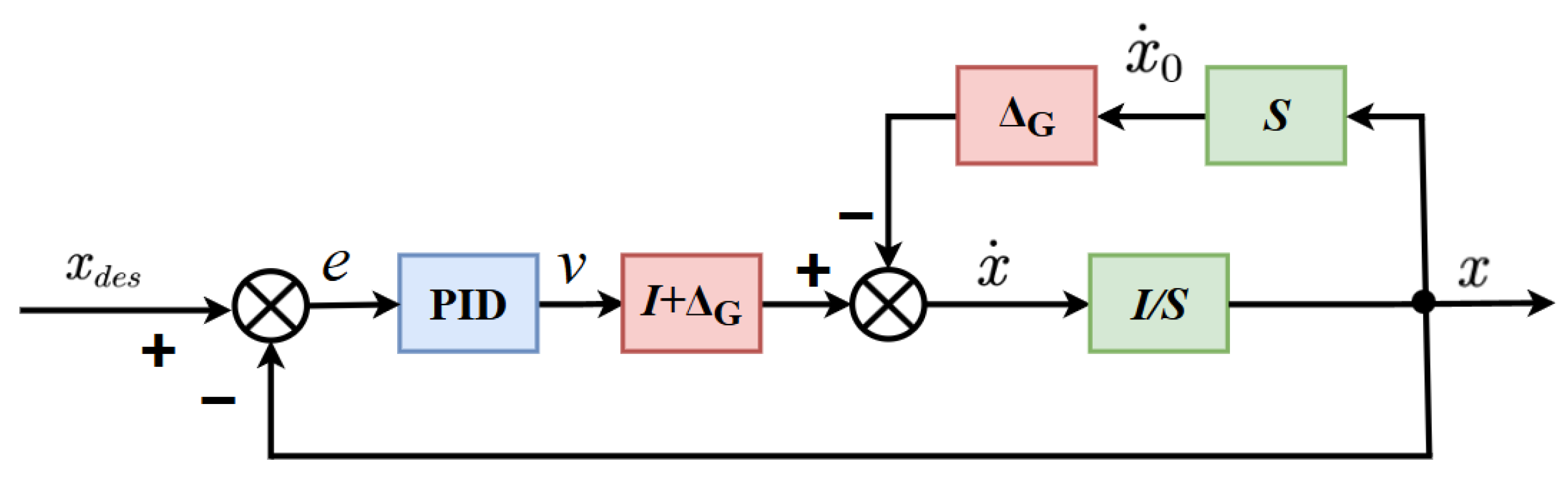
According to Equation (18), the control scheme is designed as Figure 1, where ${\Delta }_G$ denotes the model uncertainties, PID denotes Proportional Integral Derivative (PID) algorithm, and $s,I/s$ denote integration or differentiation respectively.

The pseudo-inverse control input $v(t)=(K_P+{\displaystyle \raisebox{1ex}{$K_I$}\!\left/ \!\raisebox{-1ex}{$s$}\right.}+K_{D}s)e(t)$ is obtained by PID design and the transfer function of the system (18) is defined as $G_f(s)$. The transfer function $G_f(s)$ is presented as follows:

$$G_f(s)={\displaystyle \frac{v(s)(I+{\Delta }_G)\frac{I/s}{I+s{\Delta }_G/s}}{1+(v(s)(I+{\Delta }_G)\frac{I/s}{I+s{\Delta }_G/s})}}={\displaystyle \frac{v(s)\frac{I+{\Delta }_G}{s(I+{\Delta }_G)}}{1+v(s)\frac{I+{\Delta }_G}{s(I+{\Delta }_G)}}}={\displaystyle \frac{v(s)}{s+v(s)}}$$

(19)

It can be seen that model uncertainties ${\Delta }_G=\Delta G(x_0)G^{-1}(x_0)$ in Equation (19) have been eliminated. However, the INDI method is based on Taylor’s expansion principle and the higher-order term of $\Delta H.O.T$ in Equation (11) is omit. To improve the control precision of the aircraft, the effect of higher-order terms must be considered. So, Equation (12) can be rewritten as follows:

$$\dot{x}={\dot{x}}_0+G(x_0)(u-u_0)+\Delta H.O.T$$

(20)

Therefore, it is necessary to find a method to deal with the model uncertainties due to the higher-order term $\Delta H.O.T$ of the INDI.

2.3. Problem Formulation

To realize precision control for the civil aircraft, the main objective of this study is to design a reinforcement learning-based INDI fault-tolerant controller, which meets the following requirements:

(1)

The closed-loop system is stable with model uncertainties including $\Delta H.O.T$ and actuator faults;

(2)

The system state $x$ is driven towards the desired $x_d$, and the tracking error $e=x_d-x$, meets $\lim {‖e‖}_2<\epsilon$, where the $\epsilon$ is a prescribed constant. ${‖e‖}_2=\sqrt{e^{\mathrm{T}}e}$ represents the 2-norm of the vector $e$.

3. RL-RMI-INDI-Based Controller Design

To improve attitude tracking control of a civil aircraft under actuator faults and model uncertainties, an RL-RMI-INDI-based fault-tolerant control method is proposed in this section.

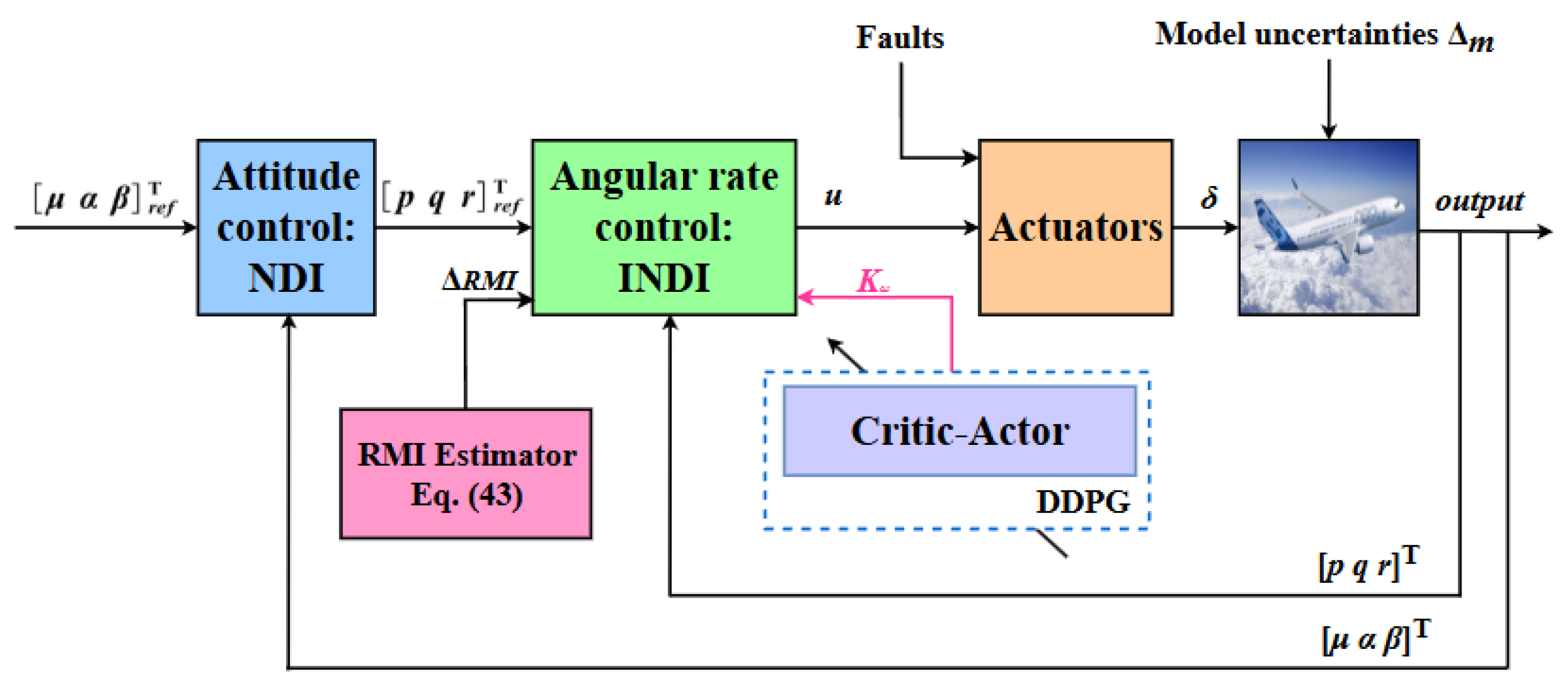
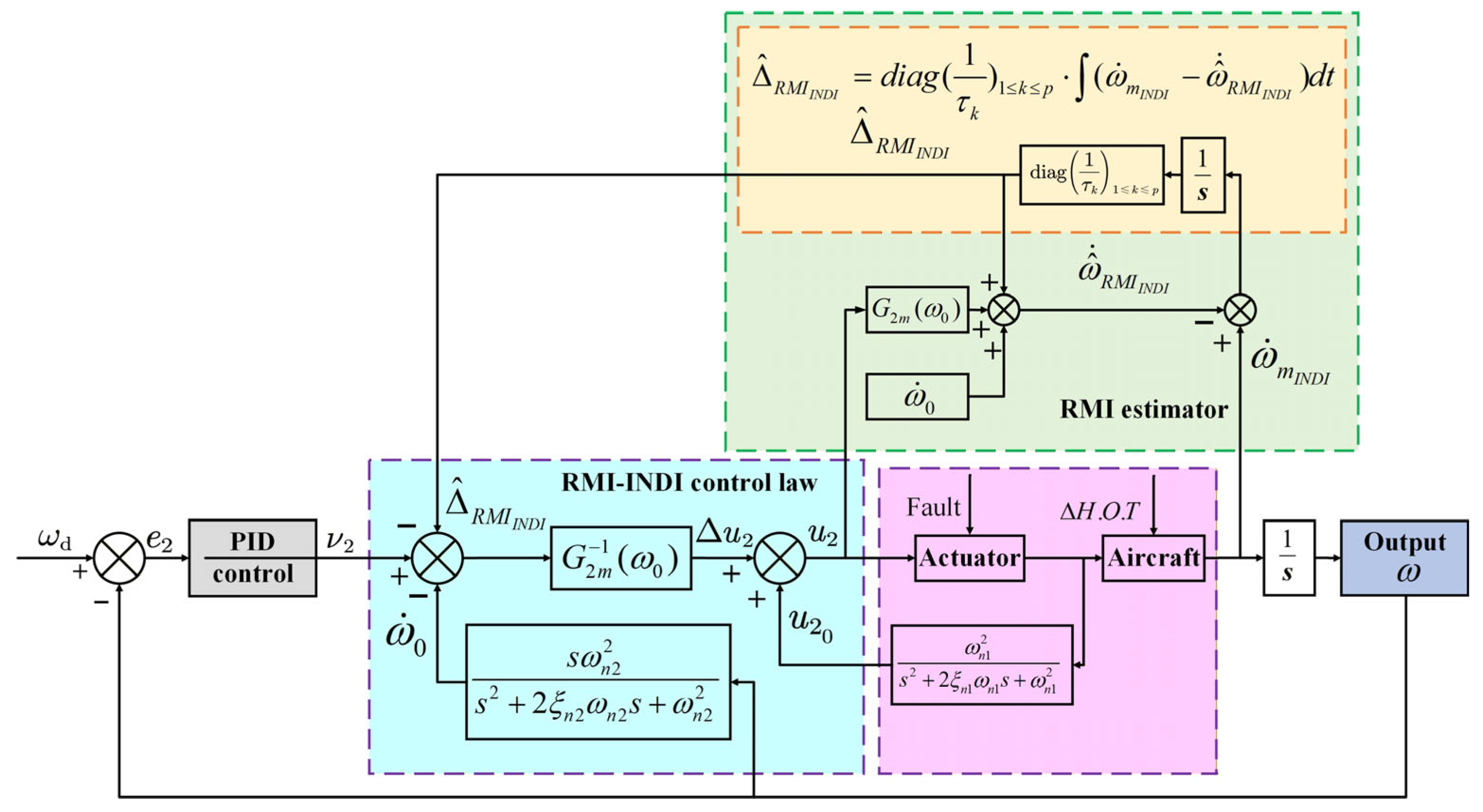
The control structure based on RL-RMI-INDI is shown in Figure 2, which includes a DDPG-based reinforcement learning loop, an update of the gain $K_{\omega }$, an attitude control loop, an angular rate control loop, and a RMI estimator.

3.1. Attitude Control Loop

The objective of the attitude control loop is to track the reference command vector $x_{1d}={\left[{\mu }_{ref},{\alpha }_{ref},{\beta }_{ref}\right]}^{\mathrm{T}}$, where ${\beta }_{ref}$ is assumed to be zero, because it is small during flight or coordinated turn. The control input is the angular rate, $u_1=x_{2d}={\omega }_d$. Since there are no model uncertainties in the attitude control loop, the NDI method is adopted [33].

$${\dot{x}}_1=f_1+G_1{u}_1=f_1+G_1{\omega }_d$$

(21)

where $x_1={\left[\mu ,\alpha ,\beta \right]}^{\mathrm{T}}$, $u_1=x_{2d}={\omega }_d={\left[p_d,q_d,r_d\right]}^{\mathrm{T}}$.

$$f_1={\left[\begin{array}{ccc}\cos \alpha \cos \beta & 0& \sin \alpha \\ \sin \beta & 1& 0\\ \sin \alpha \cos \beta & 0& -\cos \alpha \end{array}\right]}^{-1}(-T_{BV}\left[\begin{array}{c}-\dot{\chi }\sin \gamma \\ \dot{\gamma }\\ \dot{\chi }\cos \gamma \end{array}\right])$$

(22)

$$G_1={\left[\begin{array}{ccc}\cos \alpha \cos \beta & 0& \sin \alpha \\ \sin \beta & 1& 0\\ \sin \alpha \cos \beta & 0& -\cos \alpha \end{array}\right]}^{-1}$$

(23)

where $T_{BV}$ is the coordinate transformation matrix, as shown in Equation (2).

By using the dynamic inverse method, the desired angular rate can be obtained by Equation (21):

$$u_1={\omega }_d=G_1^{-1}({\dot{x}}_1-f_1)=G_1^{-1}(v_1-f_1)$$

(24)

The virtual control $v_1$ is designed by the PID control.

$$v_1=K_{P_1}{e}_1(t)+K_{I_1}{\displaystyle {\int }_0^t{e}_1(\tau )d\tau }+K_{D_1}{\displaystyle \frac{d{e}_1(t)}{dt}}$$

(25)

where the attitude error $e_1(t)=x_{1d}-x_1$, $K_{P_1},K_{I_1},K_{D_1}$ are the control parameters to be designed.

3.2. Angular Rate Control Loop

The angular rate inner loop controller structure based on the RMI-INDI is shown in Figure 3, which includes the RMI-INDI controller, a robust multiple inversion-based estimator, actuator model and aircraft model.

3.2.1. The Robust Multiple Inversion Estimator Design

Consider the angular rate system of the aircraft with model uncertainties as follows:

$${\dot{\omega }}_m=f_{2m}(\omega )+G_{2m}(\omega )u_2$$

(26)

where $f_{2m}(\omega )=f_2(\omega )+\Delta f_{2m}(\omega )$, $G_{2m}(\omega )=G_2(\omega )+\Delta G_{2m}(\omega )$, $\Delta f_{2m}(\omega )$ and $\Delta G_{2m}(\omega )$ represent the model uncertainties associated with the functions of $f_2(\cdot )$ and $G_2(\cdot )$, respectively. By using the NDI control, the control input $u_2$ is obtained as follows:

$$u_2=G_{2m}^{-1}(\omega )(v_2-f_{2m}(\omega ))$$

(27)

where $v_2$ denotes the pseudo-control input. Equation (26) can be expressed as follows:

$${\dot{\omega }}_m=f_2(\omega )+G_2(\omega )u_2+{\Delta }_m$$

(28)

where ${\Delta }_m=\Delta f_{2m}(\omega )+\Delta G_{2m}(\omega )u_2$.

To reduce the effects of model uncertainties, a novel RMI estimator system ${\dot{\widehat{\omega }}}_{RMI}$ is designed. Let ${\dot{\omega }}_{aug}=\left[\begin{array}{c}\dot{\omega }\\ {\dot{\omega }}_m\\ {\dot{\widehat{\omega }}}_{RMI}\end{array}\right]$, the augmentation system is presented as follows:

$${\dot{\omega }}_{aug}=\left[\begin{array}{c}\dot{\omega }\\ {\dot{\omega }}_m\\ {\dot{\widehat{\omega }}}_{RMI}\end{array}\right]=\left[\begin{array}{c}{f}_2(\omega )+G_2(\omega )u_2\\ f_2(\omega )+G_2(\omega )u_2+{\Delta }_m\\ f_2(\omega )+G_2(\omega )u_2+{\Delta }_m-{\Delta }_{RMI}\end{array}\right]$$

(29)

The robust multiple inversion factor ${\Delta }_{RMI}$ in Equation (29) is designed by an error integral as follows:

$${\widehat{\Delta }}_{RMI}=diag{({\displaystyle \frac{1}{{\tau }_k}})}_{1\le k\le p}\cdot {\displaystyle \int ({\dot{\widehat{\omega }}}_{RMI}-\dot{\omega })}dt=diag{({\displaystyle \frac{1}{{\tau }_k}})}_{1\le k\le p}\cdot {\displaystyle \int ({\Delta }_m-{\widehat{\Delta }}_{RMI})}dt$$

(30)

where $diag{({\displaystyle \frac{1}{{\tau }_k}})}_{1\le k\le p}=diag(1/{\tau }_1,1/{\tau }_2,\cdots ,1/{\tau }_p)$, and ${\tau }_k>0$, $k$ is the relative degree of the system, $p$ is the maximum relative degree of the system, and ${\widehat{\Delta }}_{RMI}$ is the estimated value of the robust multiple inversion factor ${\Delta }_{RMI}$.

Since the static error of the system can be eliminated by the integral control, the convergence process can be obtained by Equations (29) and (30) as follows:

$$\underset{t\to \infty }{\lim }{\widehat{\Delta }}_{RMI}(t)={\Delta }_m$$

(31)

Substituting Equation (31) into Equation (30) yields

$${\displaystyle \int ({\Delta }_m-{\widehat{\Delta }}_{RMI})}dt=0$$

(32)

According to Equations (30) and (32), ${\widehat{\Delta }}_{RMI}$ will keep un-changeable Therefore, ${\Delta }_m={\widehat{\Delta }}_{RMI}={\Delta }_{RMI}$ can be obtained, this illustrates that ${\Delta }_m$ can be estimated by the RMI-based estimator.

Substituting ${\Delta }_m={\widehat{\Delta }}_{RMI}={\Delta }_{RMI}$ into Equation (29) yields

$${\dot{\widehat{\omega }}}_{RMI}=f_2(\omega )+G_2(\omega )u_2+{\Delta }_m-{\Delta }_{RMI}=f_2(\omega )+G_2(\omega )u_2=\dot{\omega }$$

(33)

Therefore, the RMI system ${\dot{\widehat{\omega }}}_{RMI}$ is reversible.

According to the NDI control principle, the NDI control law $u_2$ of the RMI system ${\dot{\widehat{\omega }}}_{RMI}$ is as follows:

$$u_2=G_{2m}^{-1}(v_2-f_{2m}(\omega )+{\widehat{\Delta }}_{RMI})$$

(34)

where $v_2$ is the pseudo-input. Substituting ${\Delta }_m={\widehat{\Delta }}_{RMI}={\Delta }_{RMI}$ and Equation (34) into the RMI system (33) yields

$${\dot{\widehat{\omega }}}_{RMI}=f_{2m}(\omega )+G_{2m}(\omega )[G_{2m}^{-1}(v_2-f_{2m}(\omega )+{\widehat{\Delta }}_{RMI})]-{\Delta }_{RMI}=f_{2m}(\omega )+v_2-f_{2m}(\omega )+{\widehat{\Delta }}_{RMI}-{\Delta }_{RMI}=v_2$$

(35)

By using Equations (33) and (35), the following result can be obtained:

$${\dot{\widehat{\omega }}}_{RMI}=\dot{\omega }=v_2$$

(36)

In conclusion, not only ${\Delta }_m$ can be well-estimated by the RMI-based estimator, but also the feedback linearization of the system will not be affected.

3.2.2. RMI-INDI-Based the Angular Rate Fault-Tolerant Control Law Design

A. Fault-Tolerant Control of INDI

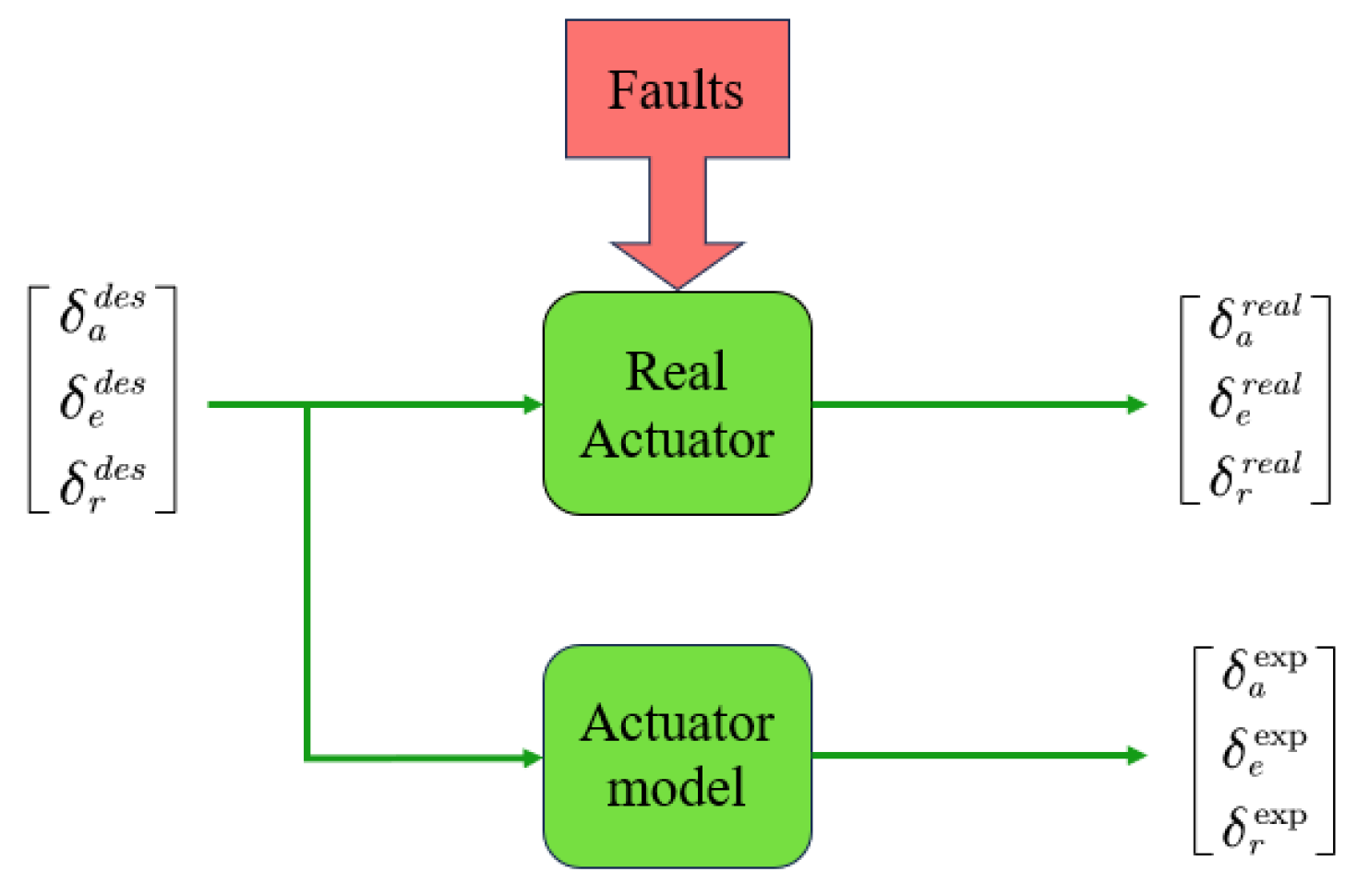
The schematic diagram of the actuator fault is shown in Figure 4.

In Figure 4, $u_{des}=({\delta }_a^{des},{\delta }_e^{des},{\delta }_r^{des})$ is the expected control variable of the control surface calculated by the controller, $u_{real}=({\delta }_a^{real},{\delta }_e^{real},{\delta }_r^{real})$ is the control surface deflection with the influence of actuator fault, and $u_{\exp }=({\delta }_a^{\exp },{\delta }_e^{\exp },{\delta }_r^{\exp })$ is the control surface deflection without actuator fault.

Taking the fault of the aileron as an example, that is:

$${\delta }_a^{real}={\lambda }_f{\delta }_a^{\exp }+{\overline{\delta }}_a^{stuck}$$

(37)

where ${\overline{\delta }}_a^{stuck}$ is the aileron stuck angle and the proportional coefficient ${\lambda }_f$ is a positive coefficient with ${\lambda }_f<1$. It can be divided into four fault cases:

(1)

${\lambda }_f=1,{\overline{\delta }}_a^{stuck}=0$: it indicates no fault on the control surface.

(2)

$0<{\lambda }_f<1,{\overline{\delta }}_a^{stuck}=0$: it indicates partial failure of the control surface.

(3)

${\lambda }_f=0,{\overline{\delta }}_a^{stuck}=0$: it indicates that the control surface has completely failed.

(4)

${\lambda }_f=0,{\overline{\delta }}_a^{stuck}\ne 0$: it indicates that the control surface is stuck.

For Case (4), an INDI-based fault tolerance control is proposed. Now consider the attitude dynamics system with actuator faults:

$$\dot{\omega }=f_2(\omega )+G_2(\omega )u_{real}$$

(38)

where the practical control input can be described as follows by Equation (11):

$$u_{real}=u_{\exp }+u^{fault}$$

(39)

Substituting Equation (39) into Equation (38) yields

$$\dot{\omega }=f_2(\omega )+G_2(\omega )(u_{\exp }+u^{fault})=f_2(\omega )+G_2(\omega )u_{\exp }+G_2(\omega )u^{fault}$$

(40)

where $u^{fault}$ is the control input generated by a single control surface with stuck fault. According to the INDI principle, and by using the Taylor expansion principle and ignoring the error of higher-order terms, Equation (40) can be rewritten as

$$\begin{array}{cc}\hfill \dot{\omega }& ={\dot{\omega }}_0+{\displaystyle \frac{\partial }{\partial \omega }}{\left(f_2(\omega )+G_2(\omega )u_{\exp }+G_2(\omega )u^{fault}\right)}_{\left|\omega ={\omega }_0,\right.u_{\exp }=u_{\exp 0},u^{fault}=u_0^{fault}}\left(\omega -{\omega }_0\right)\hfill \\ & +{\displaystyle \frac{\partial }{\partial u_{\exp }}}{\left(f_2(\omega )+G_2(\omega )u_{\exp }+G_2(\omega )u^{fault}\right)}_{\left|\omega ={\omega }_0,\right.u_{\exp }=u_{\exp 0},u^{fault}=u_0^{fault}}(u_{\exp }-u_{\exp 0})\hfill \\ & +{\displaystyle \frac{\partial }{\partial u^{fault}}}{\left(f_2(\omega )+G_2(\omega )u_{\exp }+G_2(\omega )u^{fault}\right)}_{\left|\omega ={\omega }_0,\right.u_{\exp }=u_{\exp 0},u^{fault}=u_0^{fault}}(u^{fault}-u_0^{fault})\hfill \end{array}$$

(41)

Assumption 1. 

The actuator fault type is stuck, and the fault mode is the step jump form, that is,

$$u_t^{fault}=\left\{\begin{array}{cc}0& 0<t<t_{fault}\\ {\overline{u}}^{stuck}& t_{fault}\le t\end{array}\right.$$

(42)

where $u_t^{fault}$ denotes the stuck fault of the control surface, and $t_{fault}$ is the time when the stuck fault occurs.

Define the sampling time as $\Delta t$, then $u^{fault}-u_0^{fault}$ in Equation (41) can be rewritten as

$$u^{fault}-u_0^{fault}=u_{t_{fault}+(i+1)\Delta t}^{fault}-u_{t_{fault}+i\Delta t}^{fault}(i=-1,0,1,2,3\cdots )$$

(43)

Define the actuator fault impact factor:

$${\Delta }_{fault}={\displaystyle \frac{\partial }{\partial u^{fault}}}{\left(f_2(\omega )+G_2(\omega )u_{\exp }+G_2(\omega )u^{fault}\right)}_{\left|\omega ={\omega }_0,\right.u_{\exp }=u_{\exp 0},u^{fault}=u_0^{fault}}(u^{fault}-u_0^{fault})$$

(44)

When $t=t_{fault}$, $u^{fault}-u_0^{fault}={\overline{u}}^{stuck}\ne 0$; so Equation (44) can be written as follows:

$${\Delta }_{fault}={\displaystyle \frac{\partial }{\partial u^{fault}}}{\left(f_2(\omega )+G_2(\omega )u_{\exp }+G_2(\omega )u^{fault}\right)}_{\left|\omega ={\omega }_0,\right.u_{\exp }=u_{\exp 0},u^{fault}=u_0^{fault}}{\overline{u}}^{stuck}\ne 0$$

(45)

Equation (45) indicates that the sudden actuator stuck fault impacts on the controller only at $t_{fault}$ time.

When $t\ne t_{fault}$, $u^{fault}-u_0^{fault}=0$; so Equation (44) can be written as follows:

$${\Delta }_{fault}={\displaystyle \frac{\partial }{\partial u^{fault}}}{\left(f_2(\omega )+G_2(\omega )u_{\exp }+G_2(\omega )u^{fault}\right)}_{\left|\omega ={\omega }_0,\right.u_{\exp }=u_{\exp 0},u^{fault}=u_0^{fault}}(u^{fault}-u_0^{fault})=0$$

(46)

Thus, INDI design can implement fault-tolerant control.

B. RMI-INDI-Based Angular Rate Fault-Tolerant Control Law Design

Considering the model uncertainties in the angular rate inner loop, the RMI-INDI control method is designed to achieve accurate control for angular rate. The dynamics model in the angular rate loop with model uncertainties is presented as follows:

$${\dot{\omega }}_m=f_{2m}(\omega )+G_{2m}(\omega )u_2=f_2(\omega )+G_2(\omega )u_2+{\Delta }_m=J^{-1}\left(M_0-\omega \times J\omega \right)+J^{-1}{C}_{M_u}{u}_2+{\Delta }_m$$

(47)

where $\omega ={\left[p,q,r\right]}^{\mathrm{T}}$, $u_2={\left[{\delta }_a,{\delta }_e,{\delta }_r\right]}^{\mathrm{T}}$, $f_2(\omega )\triangleq J^{-1}\left(M_0-\omega \times J\omega \right)$, $G_2(\omega )\triangleq J^{-1}{C}_{M_u}$. The first term $f_2(\omega )$ in Equation (47) indicates the uncertainties of nonlinear cross-coupling existing in the model of the angular rate model. The second term $G_2(\omega )$ represents the control effectiveness matrix. ${\Delta }_m=\Delta f_{2m}(\omega )+\Delta G_{2m}(\omega )u_2$ represents model uncertainties.

It can be found that in the INDI control law of Equation (13), the complex and variable aerodynamic moment $M_0$ in $f_2(\omega )$ is absent, which means that the INDI controller is not sensitive to the aerodynamic moment of the aircraft. Compared with NDI, the robustness of the system has been improved.

According to the Taylor series expansion, Equation (47) can be simplified as

$$\begin{array}{cc}\hfill {\dot{\omega }}_{m_{INDI}}& ={\dot{\omega }}_0+G_{2m}({\omega }_0)(u_2-u_{2_0})+\Delta H.O.T\hfill \\ & ={\dot{\omega }}_0+G_2({\omega }_0)(u_2-u_{2_0})+{\Delta }_m+\Delta H.O.T\hfill \end{array}$$

(48)

Now the RMI method can be applied to estimate and compensate for the higher-order term $\Delta H.O.T$.

Using Equation (29), the RMI-INDI system ${\dot{\widehat{\omega }}}_{RM{I}_{INDI}}$ in the angular rate loop is described as follows:

$${\dot{\widehat{\omega }}}_{RM{I}_{INDI}}={\dot{\omega }}_0+G_{2m}({\omega }_0)(u_2-u_{2_0})+{\widehat{\Delta }}_{RM{I}_{INDI}}$$

(49)

Let ${\dot{\omega }}_{aug-INDI}=\left[\begin{array}{c}{\dot{\omega }}_{INDI}\\ {\dot{\omega }}_{m_{INDI}}\\ {\dot{\widehat{\omega }}}_{RM{I}_{INDI}}\end{array}\right]$; the augmentation system is presented as follows:

$${\dot{\omega }}_{aug-INDI}=\left[\begin{array}{c}{\dot{\omega }}_{INDI}\\ {\dot{\omega }}_{m_{INDI}}\\ {\dot{\widehat{\omega }}}_{RM{I}_{INDI}}\end{array}\right]=\left[\begin{array}{c}{\dot{\omega }}_0+G_{2m}({\omega }_0)(u_2-u_{2_0})\\ {\dot{\omega }}_0+G_{2m}({\omega }_0)(u_2-u_{2_0})+\Delta H.O.T\\ {\dot{\omega }}_0+G_{2m}({\omega }_0)(u_2-u_{2_0})+{\Delta }_{RM{I}_{INDI}}\end{array}\right]$$

(50)

According to Equation (30), the RMI factor ${\Delta }_{RM{I}_{INDI}}$ in Equation (50) can be designed by the error integration as follows:

$${\widehat{\Delta }}_{RM{I}_{INDI}}=diag{({\displaystyle \frac{1}{{\tau }_k}})}_{1\le k\le p}\cdot {\displaystyle \int ({\dot{\omega }}_{m_{INDI}}-{\dot{\widehat{\omega }}}_{RM{I}_{INDI}})}dt=diag{({\displaystyle \frac{1}{{\tau }_k}})}_{1\le k\le p}\cdot {\displaystyle \int (\Delta H.O.T-{\widehat{\Delta }}_{RM{I}_{INDI}})}dt$$

(51)

where $diag{({\displaystyle \frac{1}{{\tau }_k}})}_{1\le k\le p}=diag(1/{\tau }_1,1/{\tau }_2,\cdots ,1/{\tau }_p)$, ${\tau }_k>0$, ${\widehat{\Delta }}_{RM{I}_{INDI}}$ is the estimated value of the robust multiple inversion factor ${\Delta }_{RM{I}_{INDI}}$, and the detailed RMI loop structure is shown in Figure 3.

As the above, the RMI-based estimator can effectively estimate the higher-order term $\Delta H.O.T$ in Equation (48), and by using Equation (50), the RMI-INDI-based angular rate control law $u_2$ is designed as follows:

$$u_2=u_{2_0}+\Delta u_2=u_{2_0}+G_{2m}^{-1}({\omega }_0)(v_2-{\dot{\omega }}_0-{\widehat{\Delta }}_{RM{I}_{INDI}})$$

(52)

where $\Delta u_2={\left[\Delta {\delta }_a,\Delta {\delta }_e,\Delta {\delta }_r\right]}^{\mathrm{T}}$, and the pseudo-inverse control input $v_2$ is designed as

$$v_2=K_{P_2}{e}_2(t)+K_{I_2}{\displaystyle {\int }_0^t{e}_2(\tau )d\tau }+K_{D_2}{\displaystyle \frac{d{e}_2(t)}{dt}}+{\dot{\omega }}_d$$

(53)

where ${\dot{\omega }}_d$ is the derivative of the angular rate command ${\omega }_d$, $e_2(t)={\omega }_d-{\widehat{\omega }}_{RM{I}_{INDI}}$, ${\widehat{\omega }}_{RM{I}_{INDI}}$ is the system feedback angular rate, $K_{\omega }=(K_{P_2},K_{I_2},K_{D_2})$ are control parameters to be designed.

3.3. Parameters Optimization of the RL-Based RMI-INDI Controller

To achieve the optimization of control parameters of the civil aircraft with actuator faults, a fault-tolerant control parameter optimization method is proposed based on the DDPG algorithm. DDPG is chosen because it is simple and effective in continuous control tasks that employ deterministic strategies. This method can realize adaptive parameters optimization offline for the control system and significantly improves flight control performances under actuator faults.

Since the function approximation is used by the neural network, it cannot guarantee obtaining the global optimal solution of the Hamilton–Jacobi–Bellman (HJB) equation under the strong nonlinear characteristics of aircraft dynamics. However, the proposed RL framework is to find a set of high-performance and near-optimal control gains that minimize the cumulative cost of the reward function. The objective is to significantly improve the efficiency of tuning parameters and the performance of baseline controllers.

The DDPG algorithm can be regarded as a combination of deterministic policy gradients and deep neural network; it overcomes the defects that traditional RL can only output discrete actions. Therefore, the DDPG algorithm is applied to optimize the control parameters $K_{\omega }=(K_{P_2},K_{I_2},K_{D_2})$ in Equation (53).

Reinforcement learning takes the Markov decision process as its basic framework and makes the optimal decision through the continuous interaction between the controller system and the environment [34]. The basic model can be represented by $\left\{s,a,p,R\right\}$, where $s$ represents the total set of states, $a$ represents the set of all actions, $p$ represents the probability of state transition, which is the probability that the state changes from $s_t$ to the next state $s_{t+1}$ under action $a_t$, and can be defined as $p(\left.s_{t+1}\right|s_t,a_t)$. $R$ represents the total reward function. The accumulated reward value $R_t$ during the training process is

$$R_t=r_t+\lambda r_{t+1}+{\lambda }^2{r}_{t+2}+\cdots ={\displaystyle \sum _{k=1}^{\infty }{\lambda }^k{r}_{t+k+1}}$$

(54)

where $\lambda$ is the discount factor, satisfying $\lambda \in \left[\begin{array}{cc}0& 1\end{array}\right]$, $r_t$ is the reward at the time $t$.

In the DDPG design, an actor is a deterministic policy function that can be expressed as $\pi$. The parameters of the actor network to be learned are represented as ${\theta }^{Q^{\prime }}$, and the parameters of the critic network to be learned are represented as ${\theta }^{{\mu }^{\prime }}$. Each action of the aircraft control system is directly calculated by $a_t=\mu (s_t)$ and does not need to be sampled from the random policy [35]. In the state $s_t$, the action $a_t$ is performed through policy $\pi$ to obtain the next state $s_{t+1}$ and the reward value $r_t$.

The actor network comprises two hidden layers by using the ReLU activation function, which includes 256 neurons and 128 ones, respectively. The tanh activation function is used by the output layer, and the output is scaled according to the action range. The critic network also comprises two hidden layers, which includes 256 neurons and 128 ones, respectively, and the state and action are concatenated before they are feedback to the second hidden layer.

The DDPG produce is as follows:

Step 1: Select the action according to the current policy: $a_t=\mu (\left.s_t\right|{\theta }^{\mu })$.

Step 2: Perform the action $a_t$, obtain the reward $r_t$, and the environment state changes from $s_t$ to $s_{t+1}$. Store transition $\left[s_t,a_t,r_t,s_{t+1}\right]$ in D.

Step 3: Sample a random minibatch of N transitions ${\{(s_i,a_i,r_i,s_{i+1})\}}_{i=1,\dots ,N}$ from D.

Step 4: Calculate using the target network: $y_i=r_i+\lambda Q^{\prime }(s_{i+1},\left.{\mu }^{\prime }(\left.s_{i+1}\right|{\theta }^{{\mu }^{\prime }})\right|{\theta }^{Q^{\prime }})$

Step 5: Update the current critic network by minimizing the target loss function:

$$L={\displaystyle \frac{1}{N}}{{\displaystyle \sum _i(y_i-Q(s_i,\left.a_i\right|{\theta }^Q))}}^2$$

(55)

Step 6: Update the current network by calculating the sampled policy gradient:

$${\nabla }_{{\theta }^{\mu }}{\left.\mu \right|}_{s_i}\approx {\displaystyle \frac{1}{N}}{\displaystyle \sum _i\left.{\nabla }_{a}Q(s,a\right|{\theta }^Q}{\left.)\right|}_{s=s_i,a=\mu (s_i)}{\nabla }_{{\theta }^{\mu }}\mu (s\left|{\theta }^{\mu }\right.){|}_{s_i}$$

(56)

Step 7: Update the target network by using exponential smoothing:

$$\begin{array}{ll}\hfill {\theta }^{Q^{\prime }}& \leftarrow \rho {\theta }^Q+(1-\rho ){\theta }^{Q^{\prime }}\hfill \\ \hfill {\theta }^{{\mu }^{\prime }}& \leftarrow \rho {\theta }^{\mu }+(1-\rho ){\theta }^{{\mu }^{\prime }}\hfill \end{array}$$

(57)

where $\rho \in (0,1)$ represents the learning rate.

The Algorithm 1 is as follows:

Algorithm 1 DDPG

1: Set hyperparameters: soft update factor $\rho$, reward discount factor $\lambda$.

2: Randomly initialize weight parameter ${\theta }^Q$ of the critic network $Q(\left.s_t\right|{\theta }^Q)$ and weight parameter ${\theta }^{\mu }$ of the actor network $\mu (\left.s_t\right|{\theta }^{\mu })$.

3: Initialize target networks $Q^{\prime }$ and ${\mu }^{\prime }$ with weight parameters ${\theta }^{Q^{\prime }}\leftarrow {\theta }^Q$, ${\theta }^{{\mu }^{\prime }}\leftarrow {\theta }^{\mu }$.

4: Initialize replay buffer D.

5: for episode = 1, …, M do

6: Receive initial observation $s_1$.

7: for t = 1, …, T do

8: Select the action according to the current policy: $a_t=\mu (\left.s_t\right|{\theta }^{\mu })$.

9: Perform the action $a_t$, obtain the reward $r_t$, and the environment state changes from $s_t$ to $s_{t+1}$.

10: Store transition $\left[s_t,a_t,r_t,s_{t+1}\right]$ in D.

11: Sample a random minibatch of N transitions ${\{(s_i,a_i,r_i,s_{i+1})\}}_{i=1,\dots ,N}$ from D.

12: Calculate using the target network: $y_i=r_i+\lambda Q^{\prime }(s_{i+1},\left.{\mu }^{\prime }(\left.s_{i+1}\right|{\theta }^{{\mu }^{\prime }})\right|{\theta }^{Q^{\prime }})$.

13: Update the current critic network by minimizing the target loss function: $L={\displaystyle \frac{1}{N}}{{\displaystyle \sum _i(y_i-Q(s_i,\left.a_i\right|{\theta }^Q))}}^2$

14: Update the current network by calculating the sampled policy gradient: ${\nabla }_{{\theta }^{\mu }}{\left.\mu \right|}_{s_i}\approx {\displaystyle \frac{1}{N}}{\displaystyle \sum _i\left.{\nabla }_{a}Q(s,a\right|{\theta }^Q}{\left.)\right|}_{s=s_i,a=\mu (s_i)}{\nabla }_{{\theta }^{\mu }}\mu (s\left|{\theta }^{\mu }\right.){|}_{s_i}$

15: Update the target network by using exponential smoothing: $\begin{array}{ll}\hfill {\theta }^{Q^{\prime }}& \leftarrow \rho {\theta }^Q+(1-\rho ){\theta }^{Q^{\prime }}\hfill \\ \hfill {\theta }^{{\mu }^{\prime }}& \leftarrow \rho {\theta }^{\mu }+(1-\rho ){\theta }^{{\mu }^{\prime }}\hfill \end{array}$

16: end for

17: end for

To ensure that the control parameters can achieve the desired flight control performances in cases of faults and uncertainties, thus ensuring flight safety, the DDPG method is used to optimize the control parameter $K_{\omega }=(K_{P_2},K_{I_2},K_{D_2})$ in Equation (53), The algorithm application process is as follows:

(1)

State space design

The state space represents aircraft state information and is the basis for control parameters evaluation. First, define the angular rate error:

$$e_2(t)=\left[\begin{array}{c}{e}_p\\ e_q\\ e_r\end{array}\right]=\left[\begin{array}{c}{p}_d-p\\ q_d-q\\ r_d-r\end{array}\right]$$

(58)

where ${(e_p,e_q,e_r)}^{\mathrm{T}}$ is the angular rate error, ${(p_d,q_d,r_d)}^{\mathrm{T}}$ is the angular rate, and ${(p,q,r)}^{\mathrm{T}}$ is the angular rate real-time output.

The state space based on the angular rate real-time output and angular rate error can be represented as

$$s=\left[e_p,e_q,e_r,p,q,r\right]$$

(59)

(2)

Action space design

Considering the parameter optimization of the aircraft control system in scenarios with faults and uncertainties, the action space can be defined as follows:

$$a=K_{\omega }=(K_{P_2},K_{I_2},K_{D_2})$$

(60)

The parameter $K_{\omega }$ is dynamically offline optimized in each period of $\left[\begin{array}{cc}0& \mathrm{T}\end{array}\right]$; $K_{\omega }$ is related to the action $a$ directly.

(3)

Reward function design

In this part, the current state of the aircraft is effectively evaluated by designing a composite reward function, which is designed according to the state error, the control input and state constraints. To achieve the best result of the DDPG algorithm, the novel reward function is designed as follows:

$$r_t=-w_e{\left|e_2(t)\right|}^2-w_u{\left|u_2\right|}^2-w_{\omega }\tanh (w_{\alpha }{\left|\omega (t)\right|}^2)$$

(61)

where the tracking error term $-w_e{\left|e_2(t)\right|}^2$ is used to penalize the deviation from the target angular acceleration and directly reflects the control accuracy; the control input term $-w_u{\left|u_2\right|}^2$ is used to constrain excessive deflection of the control surface and to prevent actuator saturation; the state term $-w_{\omega }\tanh (w_{\alpha }{\left|\omega (t)\right|}^2)$ is used to penalize excessive angular rates by a smooth saturation function, which can assure that the aircraft flies within the safety envelope while preventing instability in the learning process due to hard constraints; $w_e,w_u,w_{\omega },w_{\alpha }$ are configuration parameters of the reward function.

Remark 2. 

The hyperbolic tangent function $tanh(·)$ is chosen because it is smooth and bounded; these properties can effectively suppress excessive angular acceleration while discontinuous phenomenon is avoided.

3.4. Stability Analysis

By using RMI systems (50) and the control law (52), the derivative of the tracking error ${\dot{e}}_2(t)$ can be obtained as follows:

$$\begin{array}{cc}\hfill {\dot{e}}_2(t)& ={\dot{\omega }}_d-{\dot{\widehat{\omega }}}_{RM{I}_{INDI}}\hfill \\ & ={\dot{\omega }}_d-({\dot{\omega }}_0+G_{2m}({\omega }_0)\Delta u_2+{\Delta }_{RM{I}_{INDI}})\hfill \\ & ={\dot{\omega }}_d-\left[{\dot{\omega }}_0+G_{2m}({\omega }_0)G_{2m}^{-1}({\omega }_0)(v_2-{\dot{\omega }}_0-{\widehat{\Delta }}_{RM{I}_{INDI}})+{\Delta }_{RM{I}_{INDI}}\right]\hfill \\ & ={\dot{\omega }}_d-\left[{\dot{\omega }}_0+v_2-{\dot{\omega }}_0+{\Delta }_{RM{I}_{INDI}}-{\widehat{\Delta }}_{RM{I}_{INDI}}\right]\hfill \\ & ={\dot{\omega }}_d-v_2+{\widehat{\Delta }}_{RM{I}_{INDI}}-{\Delta }_{RM{I}_{INDI}}\hfill \end{array}$$

(62)

Substituting Equation (53) into Equation (62) yields

$$\begin{array}{cc}\hfill {\dot{e}}_2(t)& ={\dot{\omega }}_d-(K_{P_2}{e}_2(t)+K_{I_2}{\displaystyle {\int }_0^t{e}_2(\tau )d\tau }+K_{D_2}{\displaystyle \frac{d{e}_2(t)}{dt}})-{\dot{\omega }}_d+{\widehat{\Delta }}_{RM{I}_{INDI}}-{\Delta }_{RM{I}_{INDI}}\hfill \\ \hfill {\dot{e}}_2(t)& =-(K_{P_2}{e}_2(t)+K_{I_2}{\displaystyle {\int }_0^t{e}_2(\tau )d\tau }+K_{D_2}{\displaystyle \frac{d{e}_2(t)}{dt}})+{\widehat{\Delta }}_{RM{I}_{INDI}}-{\Delta }_{RM{I}_{INDI}}\hfill \\ \hfill {\dot{e}}_2(t)& =-(K_{P_2}{e}_2(t)+K_{I_2}{\displaystyle {\int }_0^t{e}_2(\tau )d\tau }+K_{D_2}{\dot{e}}_2(t))+{\widehat{\Delta }}_{RM{I}_{INDI}}-{\Delta }_{RM{I}_{INDI}}\hfill \\ \hfill (I+K_{D_2}){\dot{e}}_2(t)& =-K_{P_2}{e}_2(t)-K_{I_2}{\displaystyle {\int }_0^t{e}_2(\tau )d\tau }+{\widehat{\Delta }}_{RM{I}_{INDI}}-{\Delta }_{RM{I}_{INDI}}\hfill \end{array}$$

(63)

and then define $\eta ={\displaystyle {\int }_0^t{e}_2(\tau )d\tau }$, $P(t)=(I+K_{D_2})$, ${\Delta }_e={\widehat{\Delta }}_{RM{I}_{INDI}}-{\Delta }_{RM{I}_{INDI}}$, where $\dot{\eta }=e_2(t)$, ${\Delta }_e$ represents all uncertainties of the RMI system, and Equation (63) can be rewritten as follows:

$${\dot{e}}_2(t)=-P^{-1}(t)[(K_{P_2}{e}_2(t)+K_{I_2}\eta -{\Delta }_e]$$

(64)

To ensure the feasibility of stability analysis, the following assumptions are introduced:

Assumption 2. 

There exists a constant $d\ge 0$ such that $‖{\Delta }_e‖\le d$, and if the RMI estimator converges asymptotically, then $d$ can be set arbitrarily small.

Since $K_{P_2},K_{I_2},K_{D_2}$ is obtained through the RL dynamic training, it can be assumed that the $K_{P_2},K_{I_2},K_{D_2}$ are time-varying bounded gain matrices, and its rate of change is also bounded during the training process.

Assumption 3. 

There exist constants and $0<{\lambda }_m\le {\lambda }_M<\infty$ such that for all $t\ge 0$,

$${\lambda }_{m}I\le K_{P_2},K_{I_2},P(t)\le {\lambda }_{M}I$$

(65)

where $K_{P_2},K_{I_2},P(t)$ are symmetric gain matrices.

Assumption 4. 

There exists a constant $\epsilon \ge 0$, and $\epsilon$ is sufficiently small such that

$$‖\dot{P}(t)‖\le \epsilon ,‖{\dot{K}}_{P_2}(t)‖\le \epsilon ,‖{\dot{K}}_{I_2}(t)‖\le \epsilon$$

(66)

Remark 3. 

In the actual implementation of RL, these assumptions can be ensured as follows: (1) DDPG gains can be designed in the prescribed range by projection clipping of its output; (2) low-pass filtering can constrain the change rate of the DDPG updated gains; (3) the parameters of the RMI estimator can be designed reasonably.

Based on the above assumptions, the stability of the closed-loop system is proven by the Lyapunov theory. The detailed proof process is shown in the Appendix A.

4. Simulation and Analysis

In this section, the civil aircraft is used as a research model with the structural parameters shown in

Table 1. Parameters for the civil aircraft.

Parameter	Values	Unit
$m$	4500	$\mathrm{kg}$
$S$	24.99	${\mathrm{m}}^2$
$\overline{c}$	1.9910	$\mathrm{m}$
$b$	13.32500	$\mathrm{m}$
$x_{cg}$	6.340	$\mathrm{m}$
$x_{cg}^{ref}$	6.500	$\mathrm{m}$
$I_{xx}$	1.12 × 104	$\mathrm{kg}\cdot {\mathrm{m}}^2$
$I_{yy}$	2.29 × 104	$\mathrm{kg}\cdot {\mathrm{m}}^2$
$I_{zz}$	3.20 × 104	$\mathrm{kg}\cdot {\mathrm{m}}^2$
$I_{xz}$	1.93 × 103	$\mathrm{kg}\cdot {\mathrm{m}}^2$
$I_{xy},I_{yz}$	0	$\mathrm{kg}\cdot {\mathrm{m}}^2$

, where $x_{cg}$ is the center of gravity position, and $x_{cg}^{ref}$ is the reference center of gravity position.

Actuator dynamics of the civil aircraft modeled as a first-order inertial transfer function [32], $G_a(s)=1/({\tau }_{a}s+1)$, where the constant value is ${\tau }_a$, is shown in

Table 2. Actuator parameters.

Actuator	Minimum Position Values (rad)	Maximum Position Values (rad)	${\mathit{\tau }}_{\mathit{a}}(\mathit{s})$
Elevator	−0.36	0.36	14
Aileron	−0.66	0.66
Rudder	−0.40	0.40

.

The filter parameters of ${\omega }_{n1}={\omega }_{n2}=25 \mathrm{rad}/\mathrm{s}$ and ${\xi }_{n1}={\xi }_{n2}=0.8$ are shown in Figure 3. The simulation experiments are carried out under the following initial flight conditions: $V_T=90 \mathrm{m}/\mathrm{s}$, $H_0=2000 \mathrm{m}$, throttle ${\delta }_t=0.38$, initial attitude angle ${(\mu ,\alpha ,\beta )}^{\mathrm{T}}={(0,3.2,0)}^{\mathrm{T}}(\mathrm{deg})$.

4.1. Simulation of Parameter Optimization

Learning parameters of the DDPG are configured as follows: the total number of rounds M = 1000; the period of a single round $\mathrm{T}=60s$; the discount factor is $\lambda =0.99$; the replacement parameter $\rho =0.02$ of the target network, the learning rates for the actor and critic are 10⁻³ and 10⁻⁴, respectively; the replay buffer size is 10⁵ and the batch size is 64; and the reward function configuration parameters are set as $w_e=10,w_u=1,w_{\omega }=5,w_{\alpha }=0.01$.

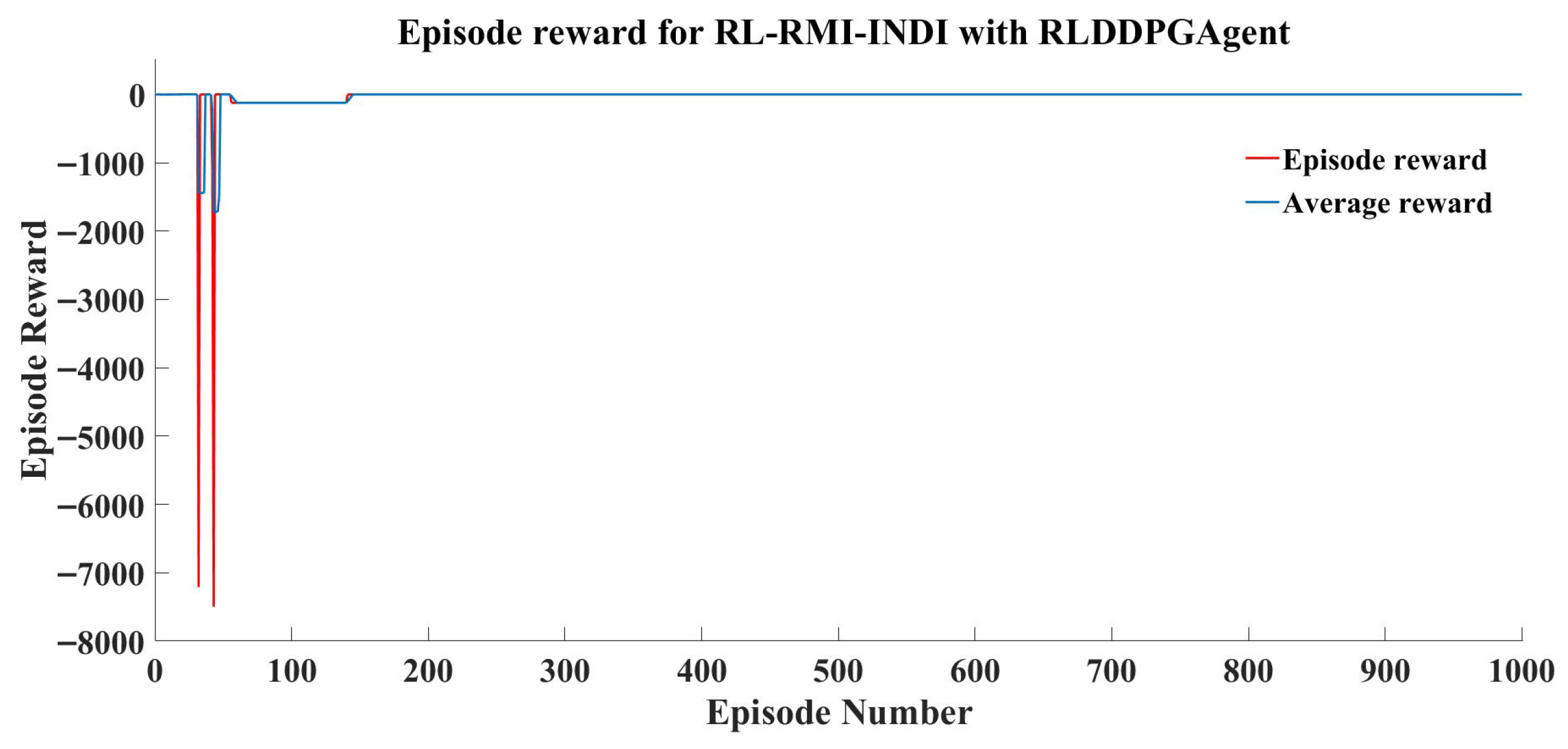
The RL training is performed offline in a simulated environment. The DDPG is used to optimize the control parameters; the training process is shown in Figure 5.

To evaluate the sensitivity of the hyperparameter of the DDPG algorithm, a series of experiments are carried out by one hyperparameter changed at a time while others are remained. The final average episode reward is recorded for each training (where more than five seeds are used). The results are summarized in

Table 3. Hyperparameter sensitivity results.

Hyperparameter	Tested Values	Final Reward (mean ± std)
Actor LR	5 × 10−4, 1 × 10−3, 5 × 10−3	−125.3 ± 4.2, −120.1 ± 3.8, −122.5 ± 5.1
Critic LR	5 × 10−5, 1 × 10−4, 5 × 10−4	−122.8 ± 4.5, −120.1 ± 3.8, −124.2 ± 4.9
Discount $\lambda$	0.95, 0.99, 0.995	−124.5 ± 4.7, −120.1 ± 3.8, −123.8 ± 5.2
Hidden neurons	[128, 64], [256, 128], [512, 256]	−121.8 ± 4.1, −120.1 ± 3.8, −119.5 ± 4.3

.

The test values of the learning rate including {10⁻⁴, 5 × 10⁻⁴, 10⁻³, 5 × 10⁻³}, and 10⁻³ (actor) and 10⁻⁴ (critic) are selected based on the convergence speed; the test range of the discount factor $\lambda$ is [0.9, 0.99]; three network structures are tested: [128, 64], [256, 128], [512, 256]; [256, 128] is selected to balance capacity and efficiency.

From Table 3, it can be seen that the algorithm remains stable within the reasonable range of these parameters, where the discount factor $\lambda$ has the greatest influence, and it remains stable within the range of $\lambda \in [0.95,0.99]$.

To verify the consistency of the RL training, a Monte Carlo simulation is carried out and the DDPG optimization process is tested by five different random seeds. The results in Table 3 show that all responses converge to a similar reward level after about 190 episodes, where a final standard deviation of the average reward is less than 8%. This demonstrates that the proposed RL algorithm is feasible and stable.

Scenario 1. 

Angular rate control loop with actuator faults.

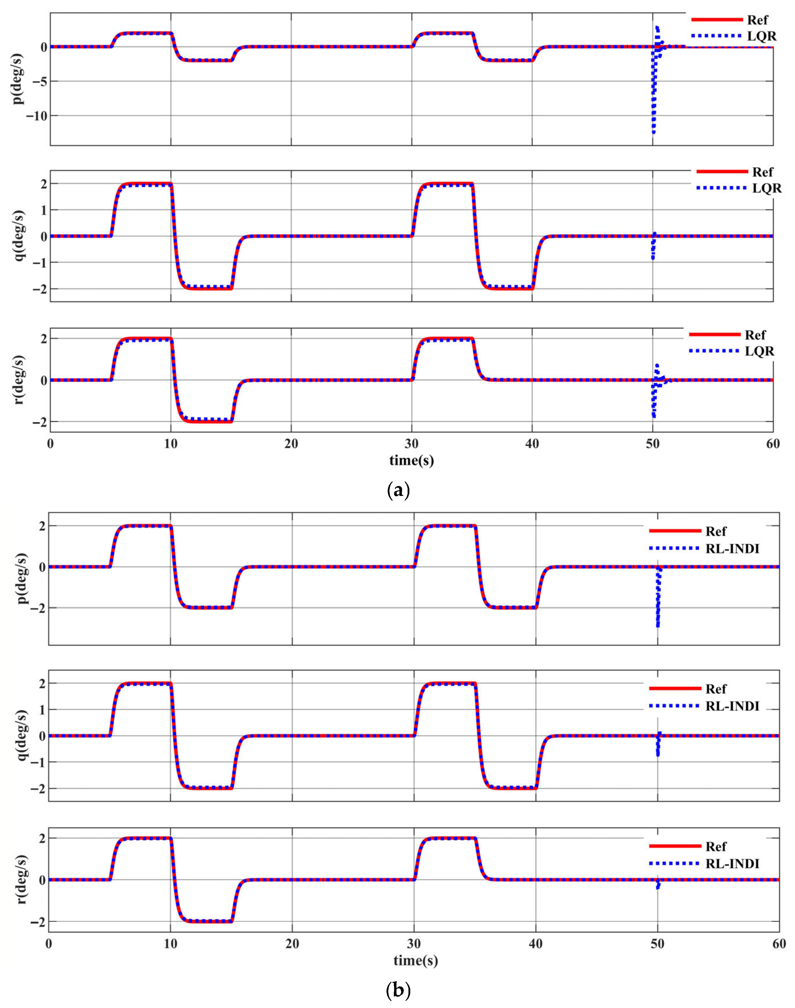
In this scenario, stuck faults of the actuators are studied, the configuration is shown in

Table 4. Actuator faults.

Time Interval	Actuator	Stuck Angle (rad)
$t>50 \mathrm{s}$	Aileron (left)	0.34
$t>50 \mathrm{s}$	Elevator (left)	0.52
$t>50 \mathrm{s}$	Rudder (upper)	0.2

.

As in Figure 6 and

Table 5. Performance comparative data under actuator faults.

Controller	Variable	Overshoot (deg/s)	Settling Time (s)
LQR	p	−13.2	1.2
	q	−0.9	0.23
	r	−1.9	1.3
RL-INDI	p	−3	0.3
	q	−0.75	0.2
	r	−0.5	0.16

, when the actuator is stuck, the tracking performances of the angular rate by the RL-INDI with fault-tolerant control are significantly better than those by the LQR design. Therefore, the RL-INDI design has better control performances for sudden faults.

4.2. Simulation of Attitude Tracking Control with Model Uncertainties and Actuator Faults

Scenario 2. 

Attitude tracking control with model uncertainties

In this Scenario, the controller parameters and the RMI time constant matrix ${\tau }_k$ of the RL-RMI-INDI controller are designed as shown in

Table 6. Controller parameters and time constant matrix.

${({\mathit{K}}_{{\mathit{P}}_1},{\mathit{K}}_{{\mathit{I}}_1},{\mathit{K}}_{{\mathit{D}}_1})}^{\mathit{T}}$	${({\mathit{K}}_{{\mathit{P}}_2},{\mathit{K}}_{{\mathit{I}}_2},{\mathit{K}}_{{\mathit{D}}_2})}^{\mathit{T}}$	${\mathit{\tau }}_{\mathit{k}}$
$\left[\begin{array}{c}{K}_{P_1}(p,q,r)\\ K_{I_1}(p,q,r)\\ K_{D_1}(p,q,r)\end{array}\right]=\left[\begin{array}{ccc}10& 10& 10\\ 0.25& 0.25& 0.25\\ 0.5& 0.5& 0.5\end{array}\right]$	$\left[\begin{array}{c}{K}_{P_2}(p,q,r)\\ K_{I_2}(p,q,r)\\ K_{D_2}(p,q,r)\end{array}\right]=\left[\begin{array}{ccc}25& 25& 50\\ 10& 5& 15\\ 1& 0.5& 2.5\end{array}\right]$	$\left[\begin{array}{ccc}20& 0& 0\\ 0& 20& 0\\ 0& 0& 6\end{array}\right]$

.

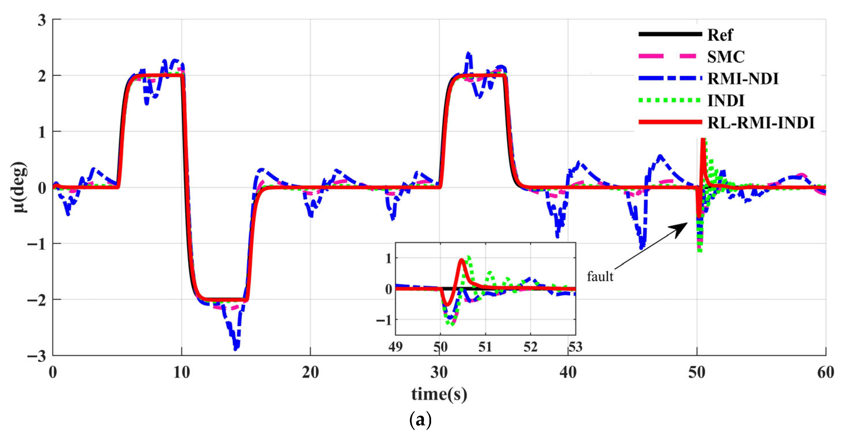
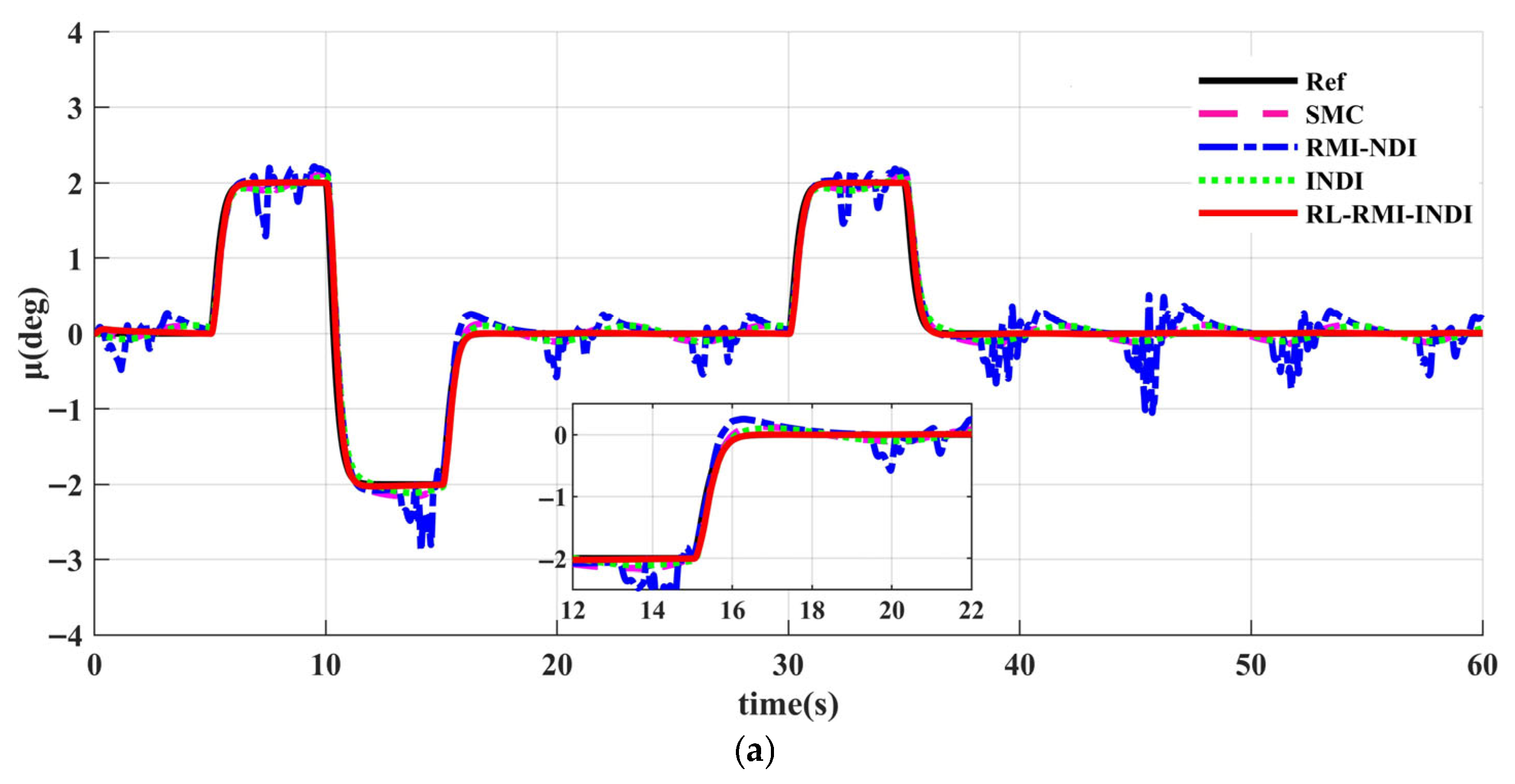
In this Scenario, an attitude tracking mission is carried out with uncertainties, the model uncertainties ${\Delta }_m$ are set as 20% reduction in the values of model parameters $m$, $I_{xx}$, $I_{yy}$, and $I_{xz}$ as shown in Table 1 and the higher-order term $\Delta H.O.T={\left[\begin{array}{ccc}0.5\sin (t)& 0.5\sin (t)& 0.5\sin (t)\end{array}\right]}^{\mathrm{T}}$. Using the proposed algorithm, the simulation results are shown in Figure 7 and Figure 8.

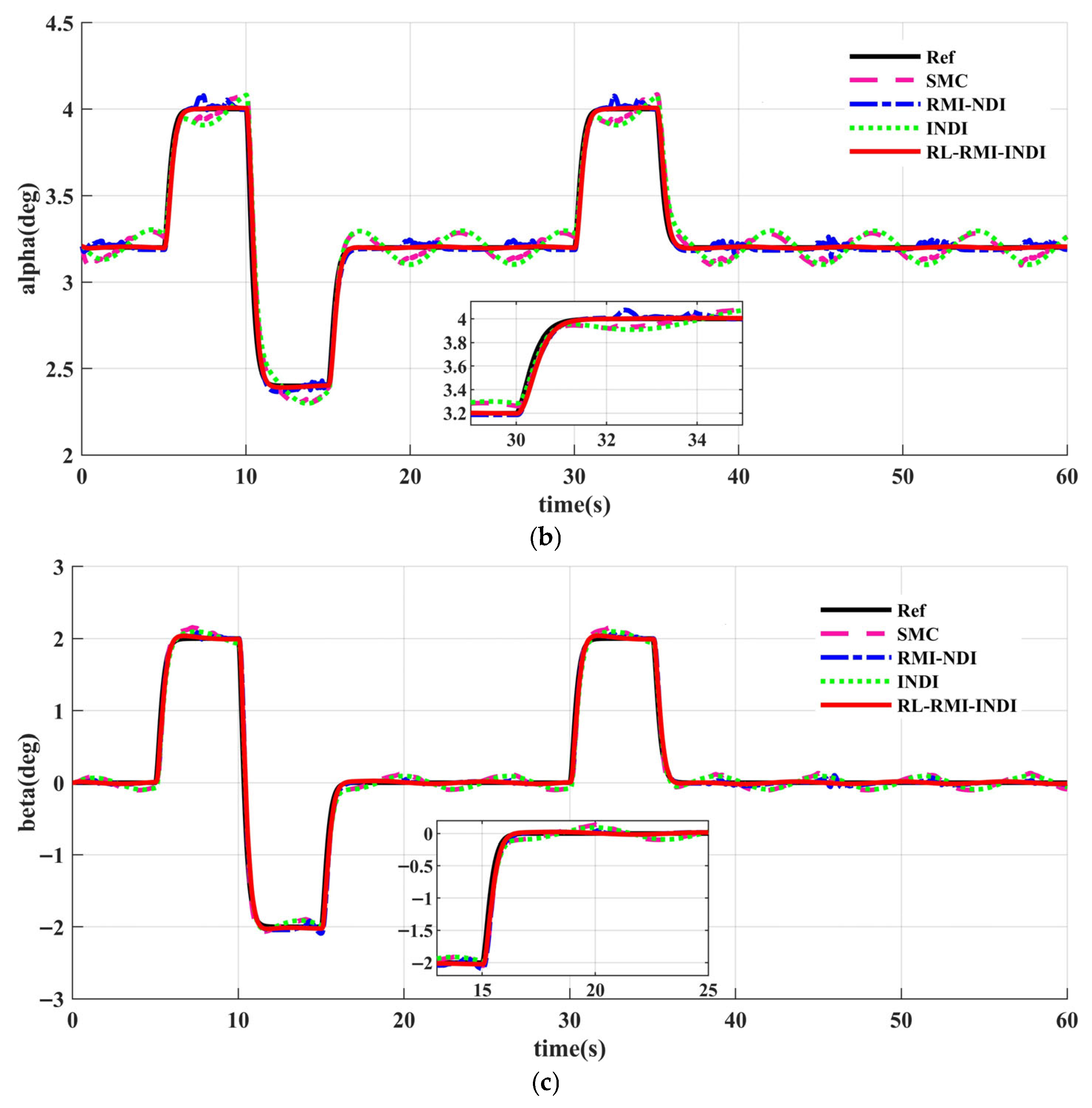
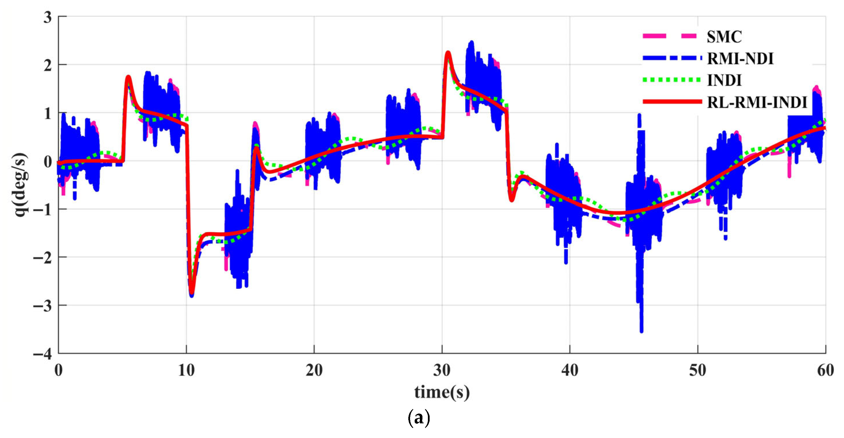
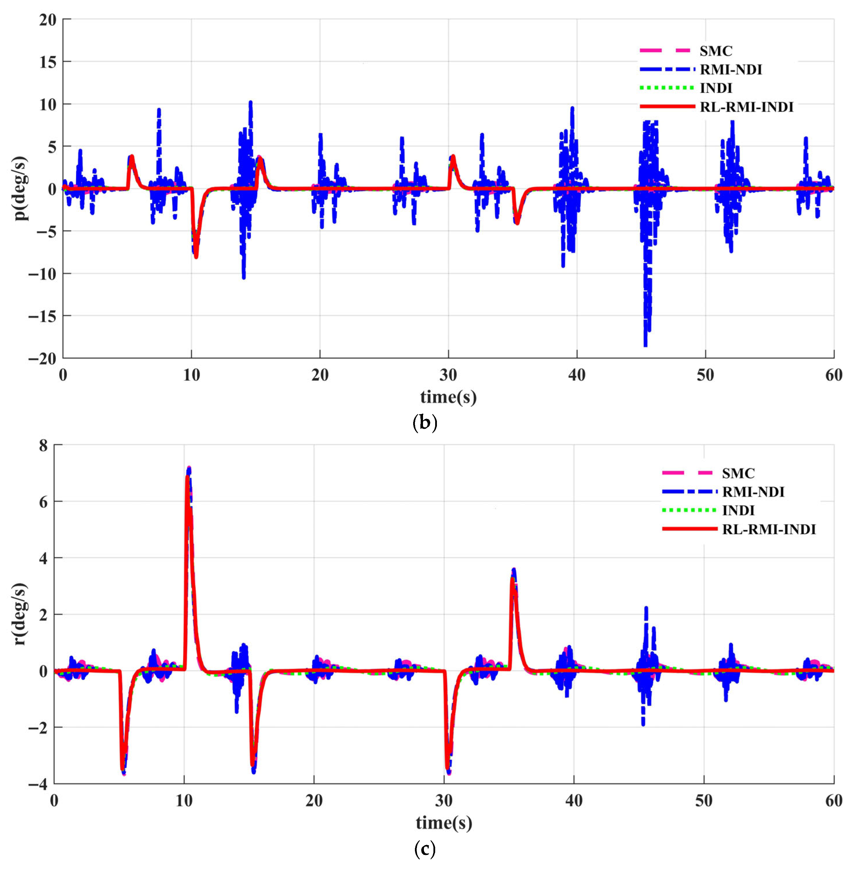
As in Figure 7 and Figure 8, the attitude tracking responses fluctuate when there are model uncertainties in the aircraft system all the time. Among which as

Table 7. Performance comparative data under uncertainties.

Controller	Variable	Overshoot (deg)	RMSE (deg)
SMC	$\mu$	−1.923	0.094
	$\alpha$	0.394	0.071
	$\beta$	0.720	0.093
RMI-NDI	$\mu$	−1.053	0.205
	$\alpha$	0.234	0.029
	$\beta$	0.735	0.065
INDI	$\mu$	−2.012	0.100
	$\alpha$	0.352	0.075
	$\beta$	0.620	0.085
RL-RMI-INDI	$\mu$	0.751	0.059
	$\alpha$	0.077	0.026
	$\beta$	0.602	0.057

, the root mean square errors of the RL-RMI-INDI are the smallest, that is E = [0.059, 0.026, 0.057] (deg), while those of the RMI-NDI are the largest, and the RMI-NDI and INDI controls are less robust in this case. Compared with the SMC, RMI-NDI, and INDI methods, the attitude tracking responses have lower overshoots by the RL-RMI-INDI, which shows it has better robust performance than the RMI-NDI and INDI designs.

Scenario 3. 

Attitude tracking control with model uncertainties and actuator faults

In this Scenario, the controller parameters and the RMI time constant matrix ${\tau }_k$ of the RL-RMI-INDI controller are designed as

Table 8. Controller parameters and time constant matrix.

${({\mathit{K}}_{{\mathit{P}}_1},{\mathit{K}}_{{\mathit{I}}_1},{\mathit{K}}_{{\mathit{D}}_1})}^{\mathit{T}}$	${({\mathit{K}}_{{\mathit{P}}_2},{\mathit{K}}_{{\mathit{I}}_2},{\mathit{K}}_{{\mathit{D}}_2})}^{\mathit{T}}$	${\mathit{\tau }}_{\mathit{k}}$
$\left[\begin{array}{c}{K}_{P_1}(p,q,r)\\ K_{I_1}(p,q,r)\\ K_{D_1}(p,q,r)\end{array}\right]=\left[\begin{array}{ccc}10& 10& 10\\ 0.25& 0.25& 0.25\\ 0.5& 0.5& 0.5\end{array}\right]$	$\left[\begin{array}{c}{K}_{P_2}(p,q,r)\\ K_{I_2}(p,q,r)\\ K_{D_2}(p,q,r)\end{array}\right]=\left[\begin{array}{ccc}25& 25& 25\\ 15& 15& 15\\ 1& 0.5& 1\end{array}\right]$	$\left[\begin{array}{ccc}20& 0& 0\\ 0& 20& 0\\ 0& 0& 6\end{array}\right]$

.

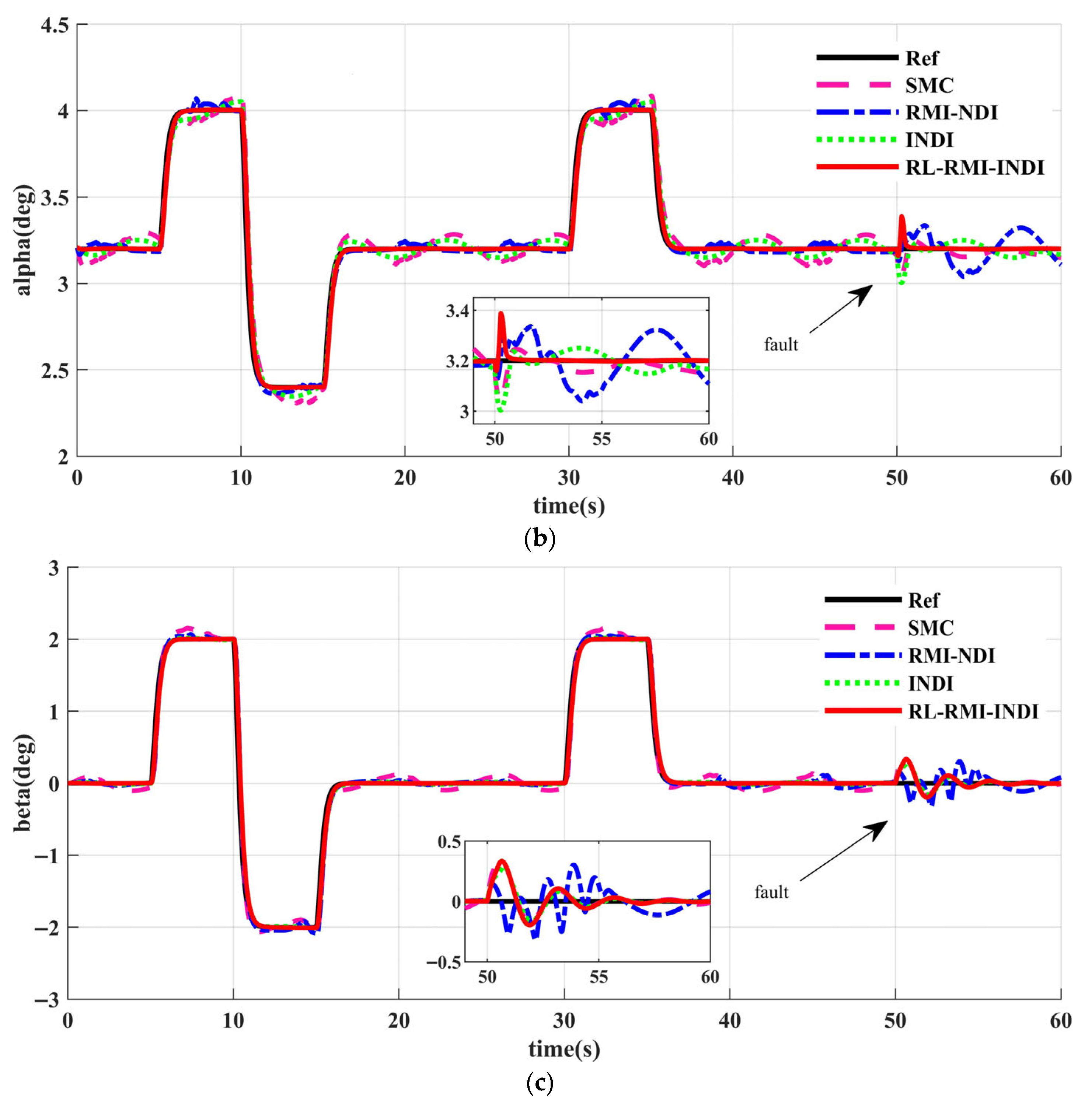
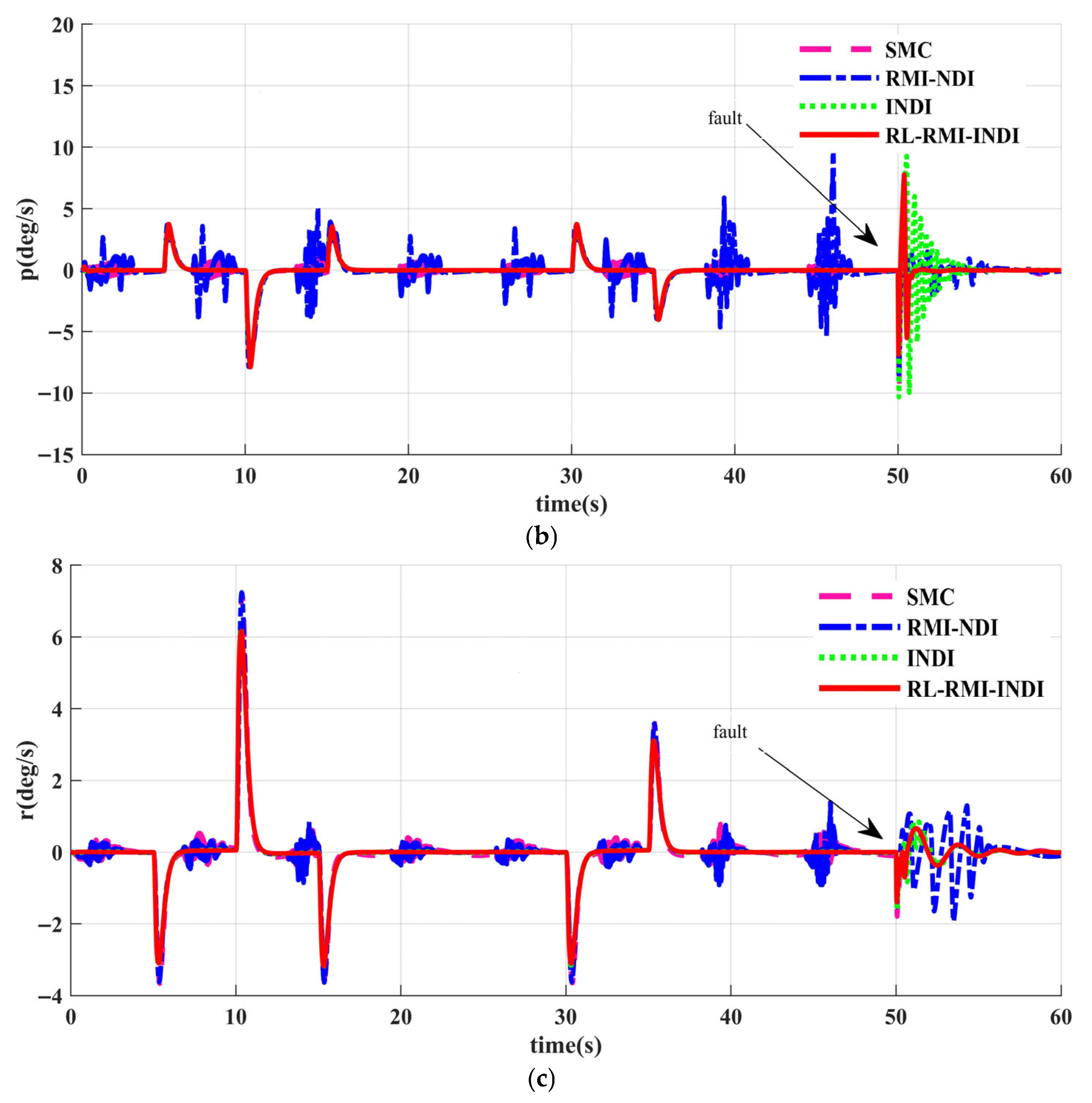
The model uncertainties ${\Delta }_m$ are set as a 20% reduction in the values of model parameters $m$, $I_{xx}$, $I_{yy}$, and $I_{xz}$ as shown in Table 1, the higher-order term $\Delta H.O.T={\left[\begin{array}{ccc}0.5\sin (t)& 0.5\sin (t)& 0.5\sin (t)\end{array}\right]}^{\mathrm{T}}$ and the specific time of fault occurrence and the angle of jamming are shown in

Table 9. Actuator faults.

Time Interval	Actuator	Stuck Angle (rad)
$t>50 \mathrm{s}$	Aileron (left)	0.28
$t>50 \mathrm{s}$	Elevator (left)	0.13
$t>50 \mathrm{s}$	Rudder (upper)	0.19

. In this scenario, the simulation results by using the proposed algorithm are shown in Figure 9 and Figure 10.

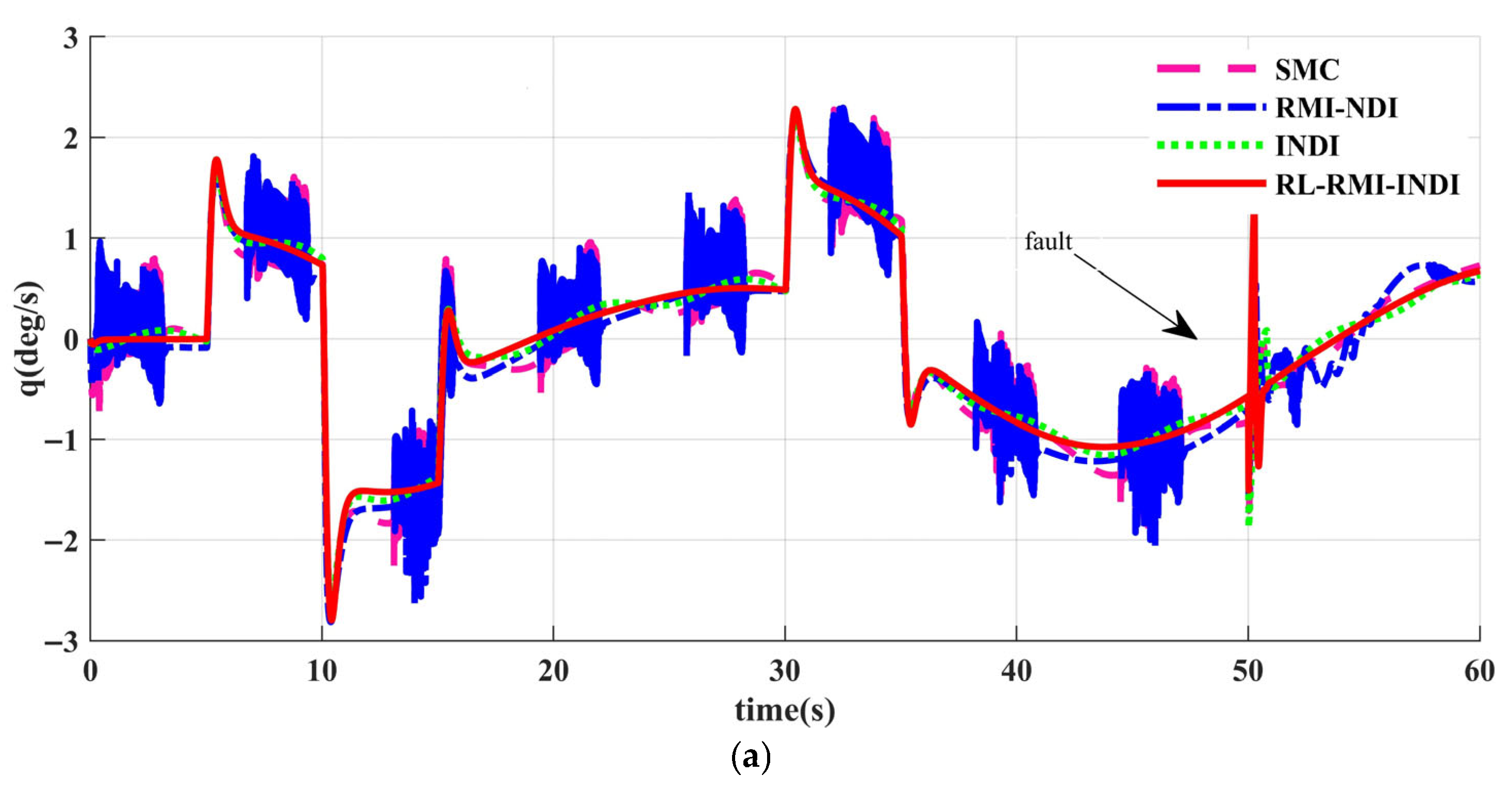
As in Figure 9 and Figure 10, the attitude tracking response initially fluctuates when the faults in elevator, aileron, and rudder occur at times of 50 s; however, the closed-loop tracking system eventually converge. Among which as

Table 10. Performance comparative data under uncertainties and actuator faults.

Controller	Variable	Overshoot (deg)	RMSE (deg)
SMC	$\mu$	−1.102	0.151
	$\alpha$	−0.132	0.043
	$\beta$	0.636	0.936
RMI-NDI	$\mu$	−1.086	0.233
	$\alpha$	0.232	0.062
	$\beta$	0.736	0.094
INDI	$\mu$	2.001	0.107
	$\alpha$	0.302	0.053
	$\beta$	0.698	0.071
RL-RMI-INDI	$\mu$	0.931	0.078
	$\alpha$	0.072	0.028
	$\beta$	0.607	0.070

, the root mean square errors of the RL-RMI-INDI are the smallest, that is E = [0.078, 0.028, 0.070] (deg), while those of the RMI-NDI are the largest; the RMI-NDI and INDI controls are less robust in this case. Compared with the SMC, RMI-NDI, and INDI methods, RL-RMI-INDI has lower overshoots, which shows that it has more robust performance than the RMI-NDI and INDI designs.

The results show that RMI effectively estimates and compensates the high-order truncation terms through its robust multi-inverse integral structure, but they are ignored in the INDI method, and thus, the RMI design can significantly improve the tracking accuracy of the system. RL uses the DDPG algorithm to adaptively optimize the controller gains and dynamically adjusts the control parameters under actuator faults; thus, the tracking accuracy of the system is effectively improved. From above, the RL-RMI-INDI architecture is proposed, which combines the estimation ability of RMI, the optimization ability of RL, and the fault-tolerant ability of INDI. The overall architecture of the RL-RMI-INDI achieves the best performance, and the effectiveness of the three parts in the proposed framework is demonstrated by the above simulations.

4.3. Flight Simulator Test

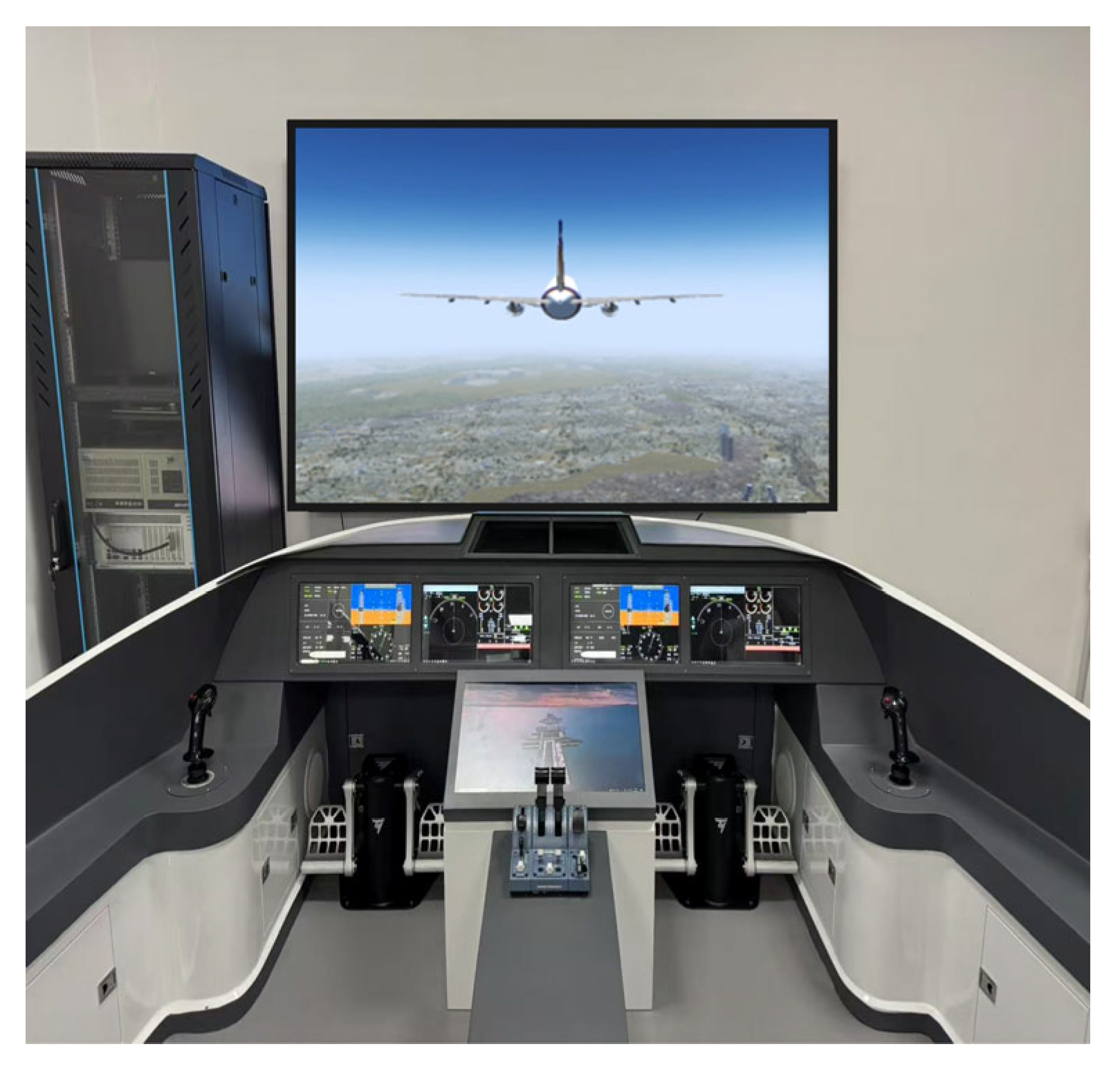
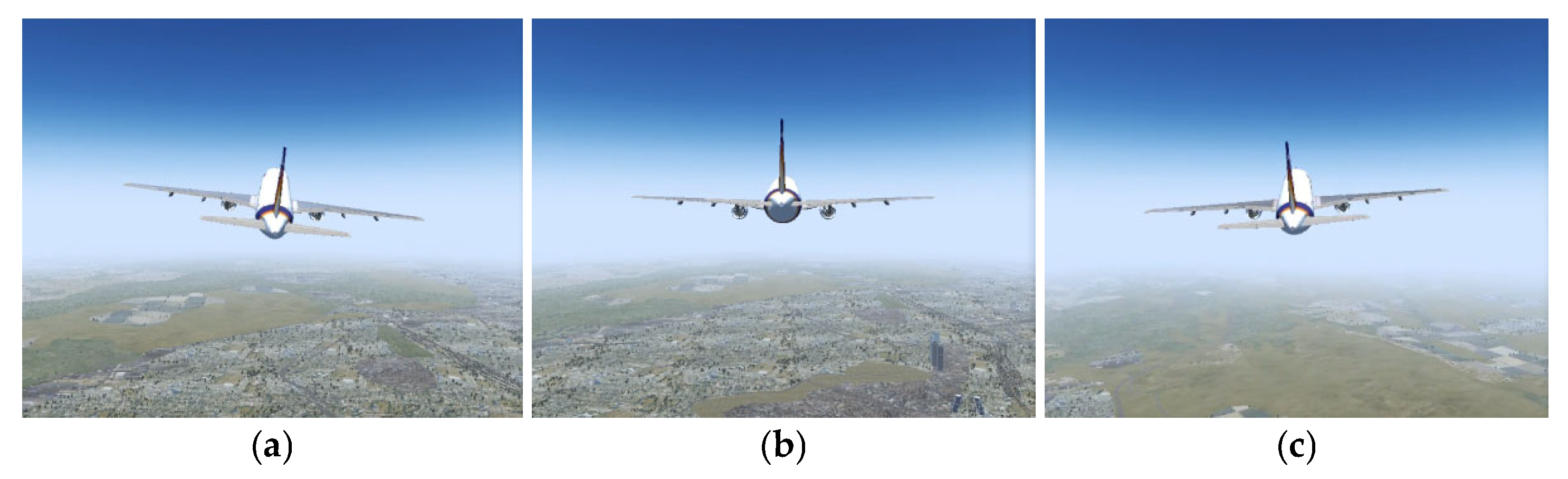
In order to simulate the practical flight environment as realistically as possible, this study conducted tests on the flight simulator in the flight control laboratory in Shanghai Jiao Tong University; the results are shown in Figure 11.

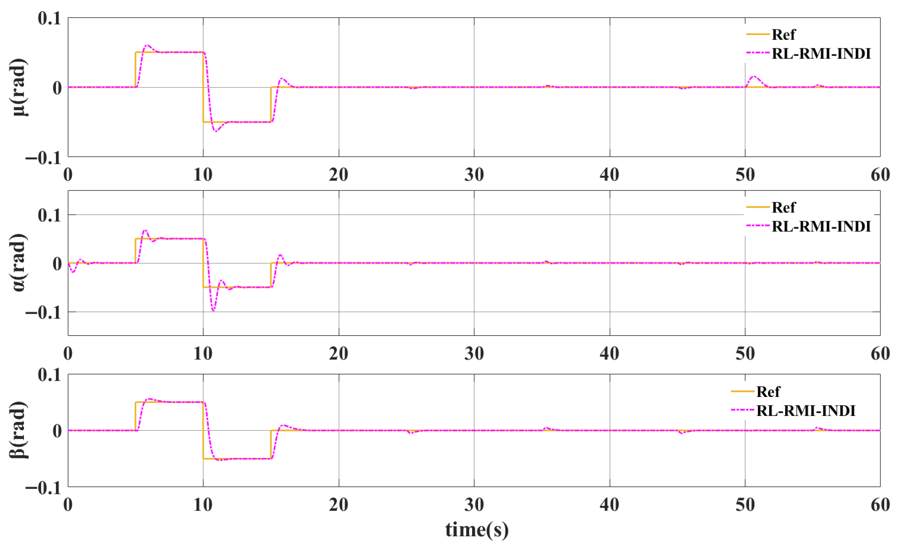
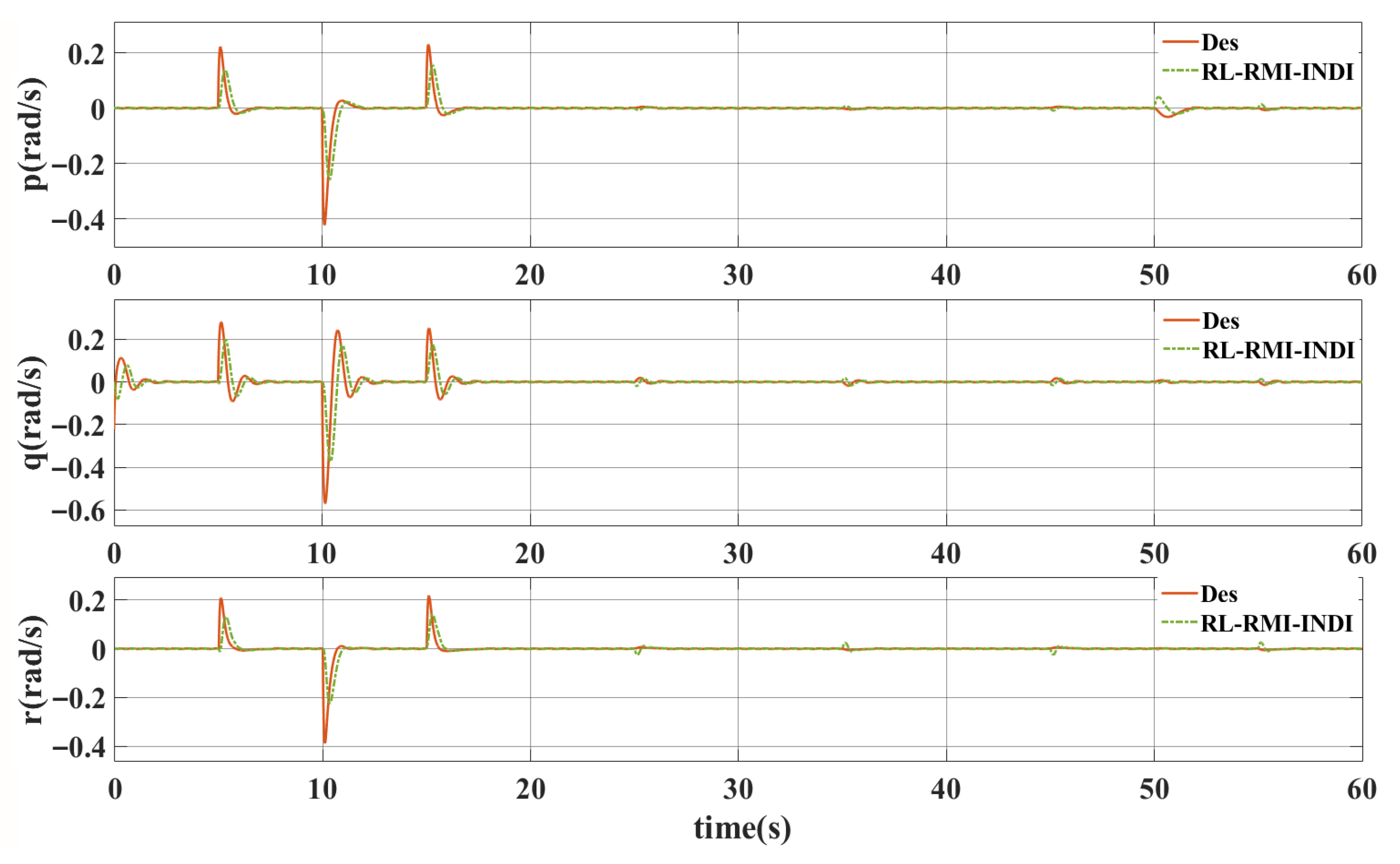
The experiments are carried out under the following initial flight conditions: $V_T=90 \mathrm{m}/\mathrm{s}$, $H_0=2000 \mathrm{m}$, and initial attitude angle of ${(\mu ,\alpha ,\beta )}^{\mathrm{T}}={(0,0,0)}^{\mathrm{T}}(\mathrm{rad})$. The actuator (left aileron) fault stuck angle of 0.12 rad $(t>50 \mathrm{s})$ and the angular rate sensor noise/fault are set as shown in

Table 11. The angular rate sensor noise/fault.

The Angular Rate Sensor	$\mathbf{Noise} {\mathit{\sigma }}_{\mathit{s}\mathit{e}\mathit{n}\mathit{s}\mathit{o}\mathit{r}}^2$	Bias Fault (rad/s)
p	10−6	0.02 $(45 \mathrm{s}>t>35 \mathrm{s})$
q	10−6	0.02 $(30 \mathrm{s}>t>20 \mathrm{s})$
r	10−6	0.02 $(15 \mathrm{s}>t>5 \mathrm{s})$

.

As in Figure 12, Figure 13 and Figure 14 and

Table 12. Simulator test data of RMSE for p, q, r.

p (rad/s)	q (rad/s)	r (rad/s)
7.6 × 10−4	7.4 × 10−4	7.3 × 10−4

, the results indicate that the proposed RL-RMI-INDI controller, combined with the signal reconstruction method based on the Kalman filter, can still maintain satisfactory performance under sensor faults. This shows that the proposed method can realize not only fault-tolerant control of actuator faults but also reconstruct the sensor faults.

5. Conclusions

A RL-RMI-INDI method is proposed to achieve fault-tolerant control of a civil aircraft. The precise attitude tracking controller is designed through two cascaded loops of attitude angle and angular rate control. The RL-RMI-INDI controller not only stabilizes the attitude and angular rate control system of the aircraft in the presence of the uncertainties but also accurately tracks the ideal attitude angular of the civil aircraft under actuator faults. In addition, robust multi-inversion is designed to estimate the uncertainties. Stability analysis indicates that the closed-loop system is stable, by the Lyapunov theory. Two scenarios of uncertainties and faults have been simulated, demonstrating the robustness of the proposed RL-RMI-INDI control. Compared with RMI-NDI and INDI controllers, the RL-RMI-INDI control can achieve more robust tracking performances under uncertainties and faults. Therefore, the effectiveness and capability of the RL-RMI-INDI design have been demonstrated. Although the effectiveness of DDPG is demonstrated by this work, future research can involve a comprehensive comparison with more advanced reinforcement learning algorithms, such as the TD3 and the SAC, and a Hardware-In-the-Loop (HIL) semi-physical simulation platform test and eventually conduct actual flight experiments in the future.

References

1. Wang, X.; Wang, S.; Yang, Z. Active fault-tolerant control strategy of large civil aircraft under elevator failures. Chin. J. Aeronaut. 2015, 28, 1658–1666. [Google Scholar] [CrossRef] [Scilit]
2. Yu, X.; Jiang, J. A survey of fault-tolerant controllers based on safety-related issues. Annu. Rev. Control 2015, 39, 46–57. [Google Scholar] [CrossRef] [Scilit]
3. Oliveira, L.; Leite, V.; Bento, A. Robust granular feedback linearization. In IEEE International Conference on Fuzzy Systems (FUZZ-IEEE); IEEE: New York, NY, USA, 2019; pp. 1–6. [Google Scholar]
4. Franco, A.L.D.; Bourlès, H. Robust Nonlinear Control Associating Robust Feedback Linearization and H∞ Control. IEEE Trans. Autom. Control 2006, 51, 1200–1207. [Google Scholar] [CrossRef]
5. Farlane, D.M.; Glover, K. A loopshaping design procedure using H∞ synthesis. IEEE Trans. Autom. Control 1992, 37, 759–769. [Google Scholar] [CrossRef] [Scilit]
6. Guillard, H.; Bourles, H. Robust feedback linearization. In Proceedings of the 14th International Symposium on Mathematical Theory of Networks and Systems, Perpignan, France, 19–23 June 2000. [Google Scholar]
7. Lavergne, F.; Villaume, F.; Jeanneau, M. Nonlinear robust Autoland. In Proceedings of the AIAA Guidance, Navigation, and Control Conference and Exhibit, San Francisco, CA, USA, 15–18 August 2005; p. AIAA 2005-5848. [Google Scholar]
8. Chakraborty, U.K. Advances in Differential Evolution; Springer Science & Business Media: New York, NY, USA, 2008. [Google Scholar]
9. Oliveira, L.; Bento, A.; Leite, V. Robust evolving granular feedback linearization. In International Fuzzy Systems Association World Congress; Springer International Publishing: Cham, Switzerland, 2019; pp. 442–452. [Google Scholar]
10. Lima, E.; Gomide, F.; Ballini, R. Participatory evolving fuzzy modeling. In International Symposium on Evolving Fuzzy Systems; IEEE: New York, NY, USA, 2006; pp. 36–41. [Google Scholar]
11. Li, Y.; Sun, L.; Qu, X. Acceleration measurement-based incremental nonlinear flight control for air-breathing hypersonic vehicles. Aerosp. Sci. Technol. 2016, 58, 235–247. [Google Scholar] [CrossRef] [Scilit]
12. Lungu, M. Backstepping and dynamic inversion combined controller for auto-landing of fixed wing UAVs. Aerosp. Sci. Technol. 2020, 96, 105526. [Google Scholar] [CrossRef] [Scilit]
13. Mullen, J.; Bailey, S.C.C.; Hoagg, J.B. Filtered dynamic inversion for altitude control of fixed-wing unmanned air vehicles. Aerosp. Sci. Technol. 2016, 54, 241–252. [Google Scholar] [CrossRef] [Scilit]
14. Wu, G.; Meng, X.; Wang, F. Improved nonlinear dynamic inversion control for a flexible air-breathing hypersonic vehicle. Aerosp. Sci. Technol. 2018, 78, 734–743. [Google Scholar] [CrossRef] [Scilit]
15. Lungu, M. Auto-landing of UAVs with variable centre of mass using the backstepping and dynamic inversion control. Aerosp. Sci. Technol. 2020, 103, 105912. [Google Scholar] [CrossRef] [Scilit]
16. Cheng, H.H.; Liu, S.Q.; Ma, X.J. Neural network incremental dynamic inversion-based trajectory tracking control of an aircraft with pilot mishandling. J. Aeronaut. Astronaut. Aviat. 2021, 53, 43–56. [Google Scholar]
17. Liu, S.Q.; Whidborne, J.F.; Lyv, W.Z.; Zhang, Q. Observer based incremental backstepping terminal sliding-mode control with learning rate for a multi-vectored propeller airship. Aerosp. Sci. Technol. 2023, 140, 108490. [Google Scholar] [CrossRef] [Scilit]
18. Rudin, K.; Ducard, G.J.J.; Siegwart, R.Y. Active fault-tolerant control with imperfect fault detection information: Applications to UAVs. IEEE Trans. Aerosp. Electron. Syst. 2019, 56, 2792–2805. [Google Scholar] [CrossRef] [Scilit]
19. Fourlas, G.K.; Karras, G.C. A survey on fault diagnosis and fault-tolerant control methods for unmanned aerial vehicles. Machines 2021, 9, 197. [Google Scholar] [CrossRef] [Scilit]
20. Solihin, M.I.; Tack, L.F.; Kean, M.L. Tuning of PID controller using particle swarm optimization (PSO). Int. J. Adv. Sci. Eng. Inf. Technol. 2011, 1, 458–461. [Google Scholar] [CrossRef] [Scilit]
21. Han, J.; Zhu, Z.; Jiang, Z. Simple PID parameter tuning method based on outputs of the closed loop system. Chin. J. Mech. Eng. 2016, 29, 465–474. [Google Scholar] [CrossRef] [Scilit]
22. Wang, Z.; Wang, Q.; He, D. An improved particle swarm optimization algorithm based on fuzzy PID control. In Proceedings of the 4th International Conference on Information Science and Control Engineering (ICISCE), Changsha, China, 21–23 July 2017; IEEE: New York, NY, USA, 2017; pp. 835–839. [Google Scholar]
23. Jiang, T.; Li, J.; Huang, K. Longitudinal parameter identification of a small unmanned aerial vehicle based on modified particle swarm optimization. Chin. J. Aeronaut. 2015, 28, 865–873. [Google Scholar] [CrossRef] [Scilit]
24. Yu, M.P.; Chong, S.H. Deploying UAV based on Reinforcement Learning for Throughput Maximization in UAV Environments. J. Kiise 2020, 47, 700–706. [Google Scholar]
25. Mo, H.; Ghulam, F. Nonlinear and adaptive intelligent control techniques for quadrotor UAV—A Survey. Asian J. Control 2019, 21, 989–1008. [Google Scholar] [CrossRef] [Scilit]
26. Ma, J.; Peng, C. Adaptive model-free fault-tolerant control based on integral reinforcement learning for a highly flexible aircraft with actuator faults. Aerosp. Sci. Technol. 2021, 119, 107204. [Google Scholar] [CrossRef] [Scilit]
27. Yang, Q.; Li, H.; Ruan, Z.; Fan, B.; Sam Ge, S. Reinforcement Learning-Based Fault-Tolerant Control of Uncertain Strict-Feedback Nonlinear Systems with Intermittent Actuator Faults. IEEE Trans. Neural Netw. Learn. Syst. 2025, 36, 10464–10478. [Google Scholar] [CrossRef] [Scilit]
28. Xie, N.; Lv, S.; Huang, Z.; Shen, H. Reinforcement learning-based fault-tolerant control of nonlinear servo systems with performance guarantees. Nonlinear Dyn. 2026, 114, 120. [Google Scholar] [CrossRef] [Scilit]
29. Liu, B.; Fu, Z.; Hua, Z.; Fang, Z.; Jing, F.; Yao, J. Reinforcement-Learning-Based Cooperative Fault-Tolerant Control for Multiactuator System with Uncertain Parameters and State Constraints. IEEE Trans. Aerosp. Electron. Syst. 2025, 61, 17084–17095. [Google Scholar] [CrossRef] [Scilit]
30. Bacon, B.; Gregory, I. General equations of motion for a damaged asymmetric aircraft. In Proceedings of the AIAA Atmospheric Flight Mechanics Conference and Exhibit, Hilton Head, SC, USA, 20–23 August 2007; p. AIAA 2007-6306. [Google Scholar]
31. Li, Y.; Liu, X.; Lu, P. Angular acceleration estimation-based incremental nonlinear dynamic inversion for robust flight control. Control Eng. Pract. 2021, 117, 104938. [Google Scholar] [CrossRef] [Scilit]
32. Lu, P.; Van, K.E.J.; De, V.C. Aircraft fault-tolerant trajectory control using incremental nonlinear dynamic inversion. Control Eng. Pract. 2016, 57, 126–141. [Google Scholar] [CrossRef] [Scilit]
33. Liu, S.Q.; Lyu, W.Z.; Zhang, Q. Neural-Network-Based Incremental Backstepping Sliding Mode Control for Flying-Wing Aircraft. J. Guid. Control Dyn. 2025, 48, 600–614. [Google Scholar] [CrossRef] [Scilit]
34. Zhang, Q.; Liu, S.Q.; Lyu, W.Z. Reinforcement Learning-Incremental Nonlinear Dynamic Inversion Based Intelligent Fault-Tolerant Control. In International Conference on Guidance, Navigation and Control; Springer Nature: Singapore, 2024; pp. 534–544. [Google Scholar]
35. Bouhamed, O.; Ghazzai, H.; Besbes, H. Autonomous UAV navigation: A DDPG-based deep reinforcement learning approach. In Proceedings of the IEEE International Symposium on circuits and systems (ISCAS), Seville, Spain, 12–14 October 2020; IEEE: New York, NY, USA, 2020; pp. 1–5. [Google Scholar]
36. Lyu, W.; Zhang, Q.; Yang, C.; Chen, J.; Liu, S.; Whidborne, J.F. LPV-Based Adaptive Robust-Augmented Control for a Blended-Wing-Body Aircraft Under Icing, Faults, Disturbances, and Uncertainties. IEEE Trans. Autom. Sci. Eng. 2026, 23, 612–630. [Google Scholar] [CrossRef] [Scilit]
Figure 1. The closed-loop control system with uncertainties.
Aerospace 13 00315 g001
Figure 2. The RL-RMI-INDI-based control structure of the civil aircraft.
Aerospace 13 00315 g002
Figure 3. Block of the RMI-INDI controller.
Aerospace 13 00315 g003
Figure 4. The schematic diagram of the actuator faults.
Aerospace 13 00315 g004
Figure 5. DDPG training process for angle rate control loop.
Aerospace 13 00315 g005
Figure 6. Angle rate tracking responses under actuator faults: (a) the output tracking responses by LQR Control; (b) the output tracking responses by the RL-INDI Control.
Aerospace 13 00315 g006
Figure 7. Attitude angle tracking responses under model uncertainties: (a) kinematic roll angle tracking responses; (b) angle of attack tracking responses; (c) sideslip angle tracking responses.
Aerospace 13 00315 g007aAerospace 13 00315 g007b
Figure 8. Angle rate tracking responses under model uncertainties: (a) pitch angle rate tracking responses; (b) roll angle rate tracking responses; (c) yaw angle rate tracking responses.
Aerospace 13 00315 g008aAerospace 13 00315 g008b
Figure 9. Attitude angle tracking responses under model uncertainties and faults: (a) kinematic roll angle tracking responses; (b) angle of attack tracking responses; (c) sideslip angle tracking responses.
Aerospace 13 00315 g009aAerospace 13 00315 g009b
Figure 10. Angle rate tracking responses under model uncertainties and faults: (a) pitch angle rate tracking responses; (b) roll angle rate tracking responses; (c) yaw angle rate tracking responses.
Aerospace 13 00315 g010aAerospace 13 00315 g010b
Figure 11. The civil aircraft simulator.
Aerospace 13 00315 g011
Figure 12. Flight process diagram of the simulator: (a) the aircraft in a rightward flight state; (b) the aircraft in a level flight state; (c) the aircraft in a leftward flight state.
Aerospace 13 00315 g012
Figure 13. Attitude angle tracking responses.
Aerospace 13 00315 g013
Figure 14. Angle rate tracking responses.
Aerospace 13 00315 g014