Adaptive Incremental Nonlinear Dynamic Inversion Control with Guaranteed Stability for Aerial Manipulators

Abstract

This paper introduces an adaptive Incremental Nonlinear Dynamic Inversion (INDI) control methodology with guaranteed stability for a highly maneuverable unmanned aerial manipulator (UAM) designed to operate under demanding conditions, such as rapid arm movements and varying manipulated payloads. This work extends previous work on the control of aerial manipulators by addressing control effectiveness uncertainties. The stability bounds of the inertia matrix within the control effectiveness matrix are derived through a detailed eigenvalue analysis, ensuring that the eigenvalues consistently remain within a specified stability threshold. The proposed methodology ensures both stability and control responsiveness by dynamically adjusting the inertia parameters of the control effectiveness matrix within stability-guaranteeing limits. The methodology is validated through extensive simulation tests showing that the proposed adaptive INDI controller outperforms previous UAM controllers, effectively coping with disturbances caused by varying grasped payloads/masses and extended arm movements with guaranteed stability.

1. Introduction

Uncrewed aerial vehicles (UAVs) have garnered substantial attention for both military and civilian applications in recent decades [1,2]. However, current UAV operations are predominantly passive, with most missions limited to observing, collecting data, or performing tasks without actively engaging or interacting with the environment or specific targets.

To expand UAV mission capabilities, researchers are integrating robotic manipulators into UAV systems, enabling them to have more dynamic and versatile interactions with their surroundings. Such enhancements would allow UAVs to perform traditionally uncommon tasks, such as clearing paths through collapsed buildings and conducting repairs in hard-to-reach industrial structures. Despite the promising potential of unmanned aerial manipulators (UAMs), their operational capabilities are currently limited by their inability to achieve fast and aggressive arm movements during flight other than hovering. Key challenges to overcome include managing changes in the UAM’s inertia parameters—such as shifts in mass, the center of mass, and the moment of inertia tensor—as well as coping with the reactionary forces and torques acting on the UAV during arm movement, especially under fast arm movements.

To address the challenge of varying inertia parameters in UAMs, researchers have developed various flight control techniques. Craig et al. in [3] addressed varying inertias and model dynamics by developing a parameter-adaptive control scheme that enhances nonlinear, model-based controllers for mechanical manipulators, ensuring uniform disturbance rejection and trajectory tracking across all configurations. Other methods focus on estimating UAV inertia parameters under different conditions, including payload additions [4], changes in the moment of inertia tensor [5], and maneuvers involving object manipulation [6]. However, these algorithms often require several seconds to converge to accurate values, which can compromise flight performance, thus limiting their applicability to simple aerial manipulation cases. Lee and Kim proposed an online parameter estimator for unknown payloads, reducing the reliance on extended convergence times [7], while Park et al. employed a Kalman filter to rapidly estimate UAM inertia parameters during manipulation maneuvers [8].

Despite efforts to manage varying inertia parameters, UAMs have yet to achieve optimal performance due to complex coupled dynamics between the UAV and manipulator. Incremental Nonlinear Dynamic Inversion (INDI) controllers [9,10,11], known for their robustness in addressing uncertainties and system coupling, are particularly suitable for complex systems such as UAMs, which involve intricate modeling and dynamic coupling formulation. INDI controllers have proven effective in UAV applications for aggressive flight control [12,13,14] and disturbance rejection [15,16,17].

Although INDI controllers are highly robust against disturbances, they require fairly comprehensive mathematical models that capture relevant information—such as geometric, inertial, and aerodynamic characteristics—typically represented in a matrix known as the control effectiveness matrix in INDI control applications. Acquiring these parameters for each system is often considered time-consuming, and they can vary in real time, particularly in UAM applications when the robotic arm moves or grasps an object. To address this challenge, Smeur et al. used a least mean squares algorithm for real-time control effectiveness matrix estimation [18], while Cao et al. combined a neural network adaptive law with INDI [19]. Similarly, Ahmadi et al. proposed a modified INDI controller to manage unmodeled dynamics resulting from actuator faults [20], and Atmaca and Kampen in [21] employed an online two-step method to estimate changes in the control effectiveness resulting from aircraft damage or faults.

Additional research has focused on INDI controllers’ robustness and stability regarding model uncertainty. Van ’t Veld et al. demonstrated that the stability of such controllers is impacted by model mismatches at different sampling times; specifically, achieving a sampling time below 0.02 s results in large stability margins [22]. Further studies have established conditions to address model mismatches in INDI controllers, ensuring bounded residual errors at high sampling frequencies [23,24,25,26]. Huang et al. in [27] found that the stability margin of an INDI controller is influenced by actuator dynamics and sampling time, which can allow for the use of relaxed model mismatch conditions. This implies that the controller can tolerate greater inaccuracies in the plant model.

In our previous reported work, INDI controllers developed for an unconventional UAV, the Navig8 aircraft, were extended to the UAM version of this aircraft [28,29,30]. In [29], a Kalman filter was used to continually estimate the control effectiveness matrix for the INDI controller without relying on information from the manipulator. Additionally, Ref. [30] presented an approach to estimate the UAM’s inertia parameters during rapid arm movements by utilizing partially known UAM parameters. This method addresses the reaction forces, moments, and rapid model variations that occur during fast arm maneuvers, particularly when grasping an unknown object in flight. While the adaptive laws in [29,30] were shown to successfully execute various UAM maneuvers, their stability was not formally guaranteed.

This paper presents an adaptive INDI control scheme for UAM systems, extending previous work to enhance the estimation of varying UAM model parameters with guaranteed stability. Similar to [30], the proposed control effectiveness matrix for the INDI controller is factored into two separate matrices but in a different formulation. One matrix is computed from known UAM parameters, while the other, ideally representing the inertia parameters of the UAM with an object in the gripper, is estimated based on a set of inequality conditions using a constrained Kalman filter. This approach ensures that the stability of the INDI controller is consistently maintained, thereby enabling the stable execution of advanced flight and robotic arm maneuvers simultaneously, whereas previous work [29,30] did not address the stability aspect.

The remainder of this paper is organized as follows: Section 2 describes the UAM system targeted in this research and outlines the general INDI control formulation for the system. Section 3 details the proposed adaptive INDI control scheme and stability analysis. Section 4 presents simulation results, and Section 5 concludes the paper with general observations.

2. INDI for UAMs

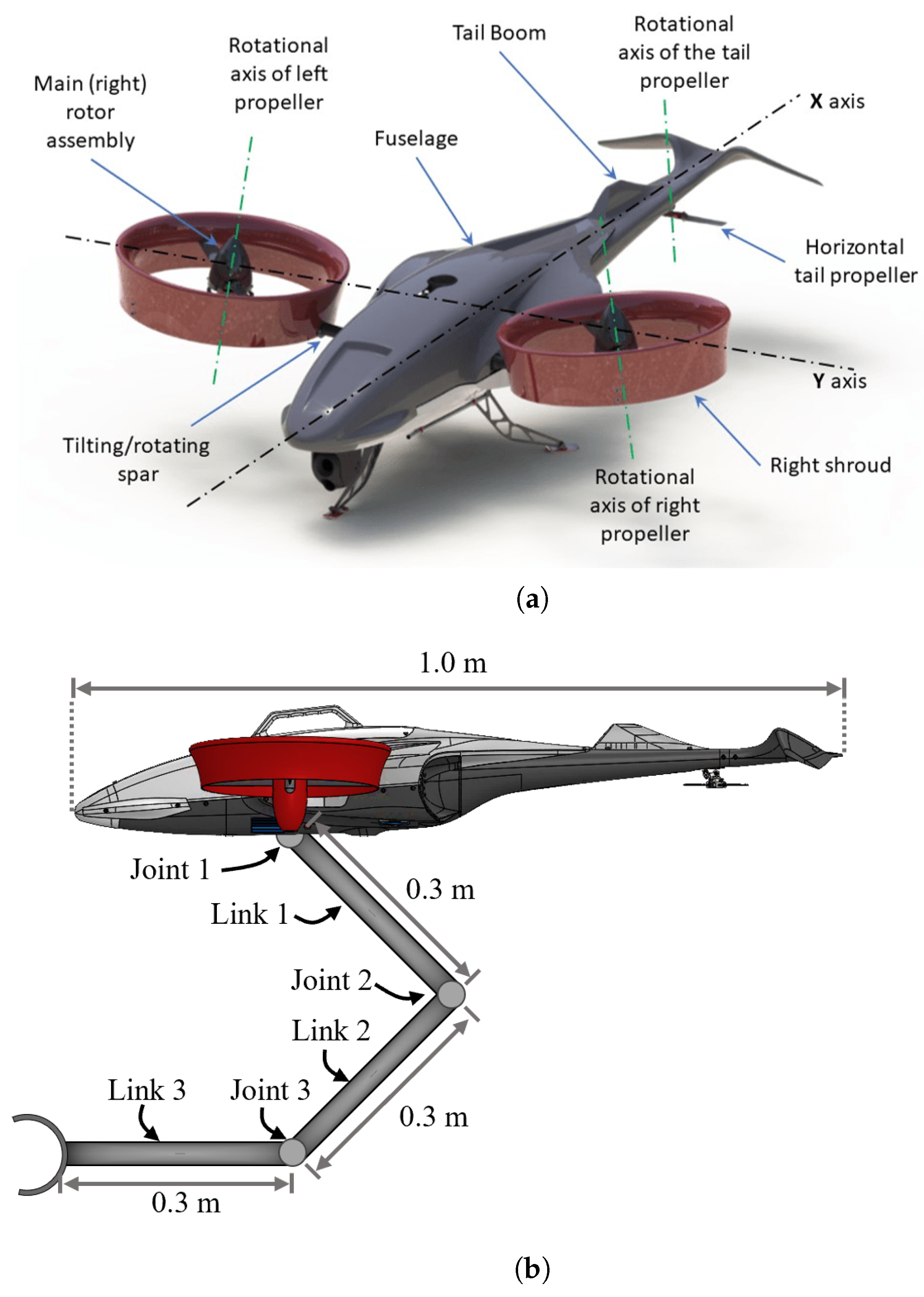
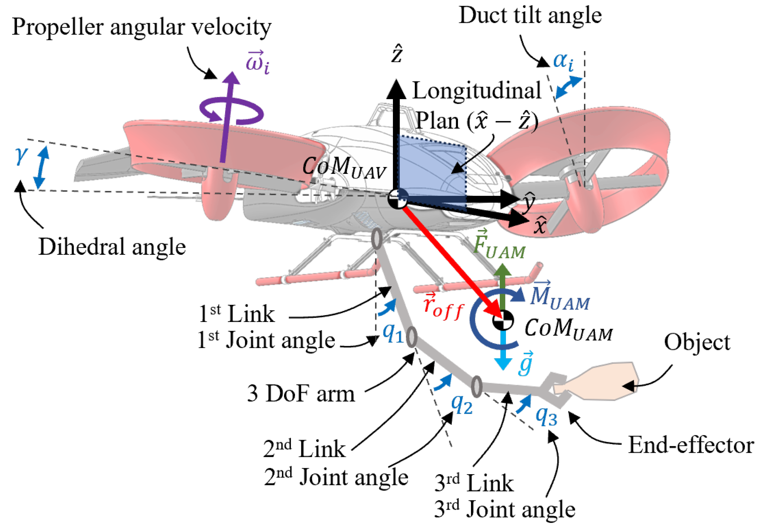
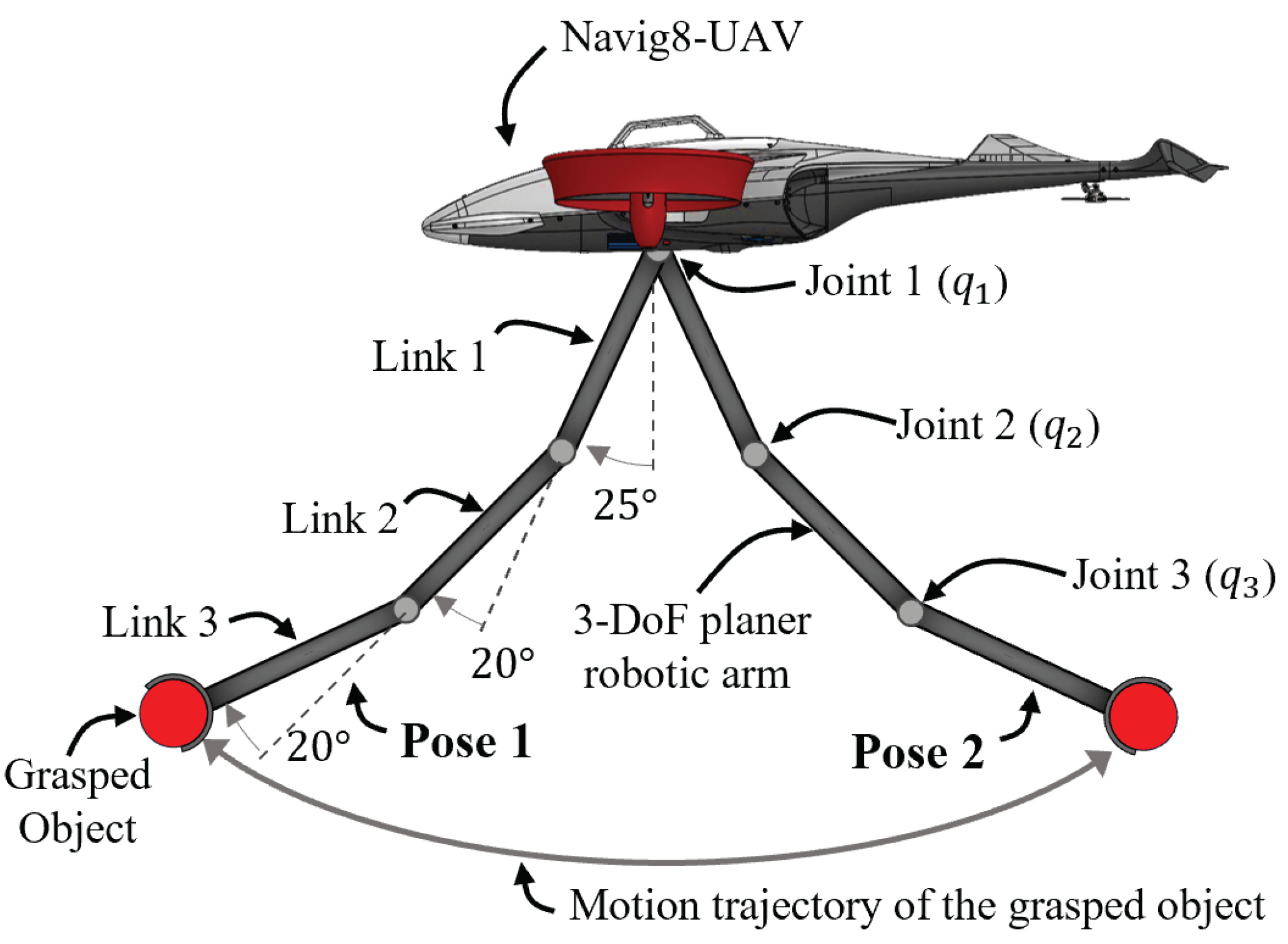
2.1. Navig8-UAM System

Although the mechanisms proposed in this paper can potentially be applied to various UAM types (e.g., helicopters and quadrotors), this research focuses on a highly maneuverable tilt-rotor VTOL vehicle, Navig8 (Figure 1a), equipped with a 3-degree-of-freedom (DoF) manipulator (Figure 1b), as the targeted dynamic system platform for analysis and testing. The Navig8-UAV, specifically designed for operations in confined spaces, is a scalable tilt rotorcraft featuring two ducted variable-pitch (VP) propellers on the left and right sides and a horizontal, non-tiltable VP tail propeller (Figure 1a). To mitigate aerodynamic effects from ground and wall proximity, the two main propellers incorporate a dihedral angle, $\gamma$, and are shrouded to enhance thrust. This configuration enables the UAV to perform unconventional, slow-speed aerobatic maneuvers that are ideal for confined-space flights, including hovering at any non-zero pitch angle. Such capabilities facilitate takeoff and landing on inclined surfaces (e.g., mountains) and allow for perching on vertical walls and ceilings.

Various control methods have been developed by the research team at the University of Calgary and 4Front Robotics Ltd. (Calgary, AB, Canada) for both the Navig8-UAV [28,31,32,33] and the Navig8-UAM [29,30,34]. The Navig8-UAM, shown in Figure 1b, integrates a 3-DoF manipulator mounted beneath the UAV, with the rotational axes of its joints aligned parallel to one another, constraining the manipulator’s movement to the longitudinal ($\widehat{x}-\widehat{z}$) plane of the UAV, as illustrated in Figure 2. The arm is equipped with an end-effector capable of grasping objects of varying sizes and weights. The Navig8-UAM is symmetric with respect to its longitudinal plane. In this research, it is assumed that accurate values for the geometric, inertial, and aerodynamic parameters of the UAM are provided. The UAV has a mass of 5 kg, with each arm linkage weighing 0.5 kg. The UAV has a body length of 1.0 m, with each arm linkage measuring 0.3 m, as shown in Figure 1b. It is important to note, however, that no information about the object to be grasped by the manipulator is provided at any time before or during flight.

2.2. INDI for UAMs

The INDI control law is derived from the force and moment equations applied to the Navig8-UAM [29]. The relationship between control input increments, $\Delta U$, and acceleration measurement increments, $\Delta Acc$, is expressed through the control effectiveness matrix G, shown in Equation (1):

$$\Delta U={\left[\begin{array}{c}{I}_{\mathrm{UAM}}^{-1}{\displaystyle \frac{\partial {\overrightarrow{M}}_{\mathrm{UAM}}}{\partial U}}\\ {\displaystyle \frac{1}{m_{\mathrm{UAM}}}}{\displaystyle \frac{\partial {\overrightarrow{F}}_{{\mathrm{UAM}}_{x,z}}}{\partial U}}\end{array}\right]}^{-1}·\Delta Acc=G^{-1}·\Delta Acc$$

(1)

where $\Delta Acc$ = $[\Delta \dot{P}$, $\Delta \dot{Q}$, $\Delta \dot{R}$, $\Delta a_x^P$, $\Delta a_z^P$]; $\dot{P}$, $\dot{Q}$, and $\dot{R}$ represent the UAV’s angular accelerations along the body axes $\widehat{x}$, $\widehat{y}$, and $\widehat{z}$, respectively; and $\Delta a_x^P$ and $\Delta a_z^P$ represent the linear accelerations along the corresponding body axes [28]. The terms $I_{\mathrm{UAM}}$ and $m_{\mathrm{UAM}}$ represent the moment of inertia and mass of the UAM, respectively, while ${\overrightarrow{M}}_{\mathrm{UAM}}$ and ${\overrightarrow{F}}_{\mathrm{UAM}}$ represent the torques and forces generated by the propellers acting on the UAM’s center of mass (CoM).

By applying the inverse rules of matrix algebra, the inverse control effectiveness matrix $G^{-1}$ can be decomposed into two matrices, $G_C^{-1}$ and $G_I$, as shown in Equation (2), where $G_C^{-1}$ is a 5 by 5 matrix that includes the parameters of the UAM, as well as the position of its CoM, and $G_I$ is a 5 by 5 matrix containing the UAM’s moment of inertia tensor and mass parameters [30].

$$\begin{array}{cc}{G}^{-1}& ={\left[\begin{array}{c}{\displaystyle \frac{\partial {\overrightarrow{M}}_{\mathrm{UAM}}}{\partial U}}\\ {\displaystyle \frac{\partial {\overrightarrow{F}}_{{\mathrm{UAM}}_{x,z}}}{\partial U}}\end{array}\right]}^{-1}·\left[\begin{array}{cc}{I}_{\mathrm{UAM}}& 0_{3\times 2}\\ 0_{2\times 3}& \left[\begin{array}{cc}{m}_{\mathrm{UAM}}& 0\\ 0& m_{\mathrm{UAM}}\end{array}\right]\end{array}\right]\\ \hfill & =G_C^{-1}·G_I\hfill \end{array}$$

(2)

The control effectiveness matrix is determined by the geometric and inertial properties of the system. However, these characteristics vary over time due to changes in the UAM’s operation, such as during a grasping task. In previous research, the inverse of the control effectiveness matrix for the given UAM system was estimated as an integrated whole to implement the INDI controller in UAM systems, without detailed knowledge of the manipulator or the object involved [29]. Furthermore, the inertia matrix ($G_I$) was estimated using the $G_C^{-1}$ matrix, which was calculated based on partially informed UAM parameters [30]. Despite these efforts, the stability of such controllers was not guaranteed.

2.3. Stability Criterion for INDI

Several studies have examined the robustness and stability of INDI controllers in the presence of control effectiveness model mismatches [22,23,24,25,26,27]. In the literature, the following proposition was established using a stability analysis of Neutral Functional Differential Equations (NFDEs) with a time delay, reformulated from INDI-controlled systems without considering actuator dynamics:

Proposition 1

([27]). G is a control effectiveness matrix obtained from the system’s true information, and $\widehat{G}$ is the corresponding estimated matrix. Assume that the square matrix $\widehat{G}{G}^{-1}$ is diagonalizable and has non-zero eigenvalues denoted by ${\lambda }_i$. Then, the necessary condition for the INDI-controlled system with the time delay to be stable is that the real part of all its eigenvalues satisfies $Re\left({\lambda }_i\right)>0.5$.

Furthermore, research has shown that the stability condition in Proposition 1 can be relaxed when actuator dynamics are included [27]. The relaxed stability analysis of the proposed INDI controller presented in this paper addresses control effectiveness uncertainties, accounting for actuator dynamics, as well as the sampling time and low-pass filters used to mitigate sensor noise, as discussed in Section 3.2.

3. Adaptive INDI with Guaranteed Stability

As described in Proposition 1, there exists a specific stability condition for the INDI controller concerning control effectiveness uncertainty. This section introduces a novel adaptive INDI control law that guarantees the stability of the INDI controller in the presence of uncertainties within the control effectiveness matrix.

For the proposed adaptive INDI control law, the control effectiveness matrix $\widehat{G}$ is formulated as per Equation (3):

$$\widehat{G}=K·G_{I_{\mathrm{UAM}}}^{-1}·G_{C_{\mathrm{UAM}}}$$

(3)

where K is a 5 by 5 positive real diagonal weighting factor matrix composed of four distinct weighting factors, represented as $K=\mathrm{diag}(K_1,K_2,K_3,K_4,K_4)$. To effectively constrain the estimation parameters within $\widehat{G}$, the control effectiveness matrix $\widehat{G}$ is partitioned differently from the method used in previous research [30], thereby ensuring the stability of the proposed INDI controller. Although a different number of weighting factors, $K_i$, can be used, only four weighting factors are used here, as they apply to the three moments of inertia and the total mass, leading to the four inertia parameters to be estimated (i.e., ${\widehat{I}}_{xx}$, ${\widehat{I}}_{yy}$, ${\widehat{I}}_{zz}$, and $\widehat{m}$). The subscript UAM in the matrices $G_{I_{\mathrm{UAM}}}^{-1}$ and $G_{C_{\mathrm{UAM}}}$, defined in Equation (2), is used to denote that such matrices are for the UAM and not for the UAV used in prior work. Such matrices are constructed using the actual UAM parameters without considering an object in the gripper. As a result, the inverse of the proposed control effectiveness matrix is formulated as Equation (4), where the inverse of the weighting factors, $K^{-1}$, is multiplied by the inertia parameters of the UAM, $G_{I_{\mathrm{UAM}}}$, creating a new inertia matrix, ${\widehat{G}}_I$, representing the updated inertia matrix of the UAM after it has grasped any unknown object (e.g., ${\widehat{I}}_{xx}={\displaystyle \frac{I_{{\mathrm{UAM}}_{xx}}}{K_1}}$, $\widehat{m}={\displaystyle \frac{m_{\mathrm{UAM}}}{K_4}}$).

$$\begin{array}{cc}\hfill {\widehat{G}}^{-1}& =G_{C_{\mathrm{UAM}}}^{-1}·G_{I_{\mathrm{UAM}}}·K^{-1}\hfill \\ \hfill & =G_{C_{\mathrm{UAM}}}^{-1}·\left[\begin{array}{ccccc}{\displaystyle \frac{I_{{\mathrm{UAM}}_{xx}}}{K_1}}& 0& {\displaystyle \frac{I_{{\mathrm{UAM}}_{xz}}}{K_3}}& 0& 0\\ 0& {\displaystyle \frac{I_{{\mathrm{UAM}}_{yy}}}{K_2}}& 0& 0& 0\\ {\displaystyle \frac{I_{{\mathrm{UAM}}_{xz}}}{K_1}}& 0& {\displaystyle \frac{I_{{\mathrm{UAM}}_{zz}}}{K_3}}& 0& 0\\ 0& 0& 0& {\displaystyle \frac{m_{\mathrm{UAM}}}{K_4}}& 0\\ 0& 0& 0& 0& {\displaystyle \frac{m_{\mathrm{UAM}}}{K_4}}\end{array}\right]\hfill \\ \hfill & =G_{C_{\mathrm{UAM}}}^{-1}·\left[\begin{array}{ccccc}{\widehat{I}}_{xx}& 0& {\widehat{I}}_{xz}& 0& 0\\ 0& {\widehat{I}}_{yy}& 0& 0& 0\\ {\widehat{I}}_{zx}& 0& {\widehat{I}}_{zz}& 0& 0\\ 0& 0& 0& \widehat{m}& 0\\ 0& 0& 0& 0& \widehat{m}\end{array}\right]\hfill \\ \hfill & =G_{C_{\mathrm{UAM}}}^{-1}·{\widehat{G}}_I\hfill \end{array}$$

(4)

It should be noted that ${\widehat{G}}_I$ is asymmetrically structured, differing from the actual system’s inertia matrix due to the formulation by the multiplication of $G_{I_{\mathrm{UAM}}}$ and $K^{-1}$. This inertia matrix, ${\widehat{G}}_I$, is estimated directly using a constrained Kalman filter, described in Section 3.3, which accounts for the simultaneous maneuvers of both the UAV and the manipulator. Although $\widehat{G}$ ideally represents the inertia matrix for the UAM system with an unknown object, it may not match the true inertia matrix exactly, as it changes and needs to be adjusted based on real-time UAM maneuvers.

The control input increment for the INDI controller ($\Delta U$) is thus formulated as per Equation (5) using the proposed control effectiveness matrix:

$$\Delta U=G_{C_{\mathrm{UAM}}}^{-1}·{\widehat{G}}_I·\Delta Acc$$

(5)

The INDI control input vector is then formulated as per Equation (6):

$$U=U_0+\Delta U$$

(6)

where $U_0$ represents the control inputs derived from the actuator output measurements (i.e., $U_0$ = $[\cos {\alpha }_{1_0}{\omega }_{1_0}^2$, $sin{\alpha }_{1_0}{\omega }_{1_0}^2$, $cos{\alpha }_{3_0}{\omega }_{3_0}^2$, $sin{\alpha }_{3_0}{\omega }_{3_0}^2$, $\mathrm{sign}\left({\omega }_{2_0}\right){\omega }_{2_0}^2{]}^T$, where ${\omega }_{1_0}$, ${\omega }_{2_0}$, and ${\omega }_{3_0}$ are the propeller angular speed measurements, and ${\alpha }_{1_0}$ and ${\alpha }_{3_0}$ are the duct tilt angle measurements processed through a low-pass filter to reduce noise).

Figure 3 illustrates the overall proposed adaptive INDI control structure for the UAM. In the adaptive law section, enclosed within the purple dashed-line box in Figure 3, $G_{C_{\mathrm{UAM}}}^{-1}$ is computed based on the angular pose of the manipulator, utilizing the provided UAM parameters [30]. ${\widehat{G}}_I$ is then estimated using the calculated $G_{C_{\mathrm{UAM}}}^{-1}$ matrix along with the available sensor measurements from the UAV and arm while taking into account the maneuvers that the UAM undergoes. In order to ensure the stability of the proposed INDI controller with respect to the control effectiveness matrix, the estimation of ${\widehat{G}}_I$ must satisfy any required inequality constraints, as detailed in Section 3.2 and Section 3.3. The combination of the estimated ${\widehat{G}}_I$ and the calculated $G_{C_{\mathrm{UAM}}}^{-1}$ matrices is then used in the INDI control law (red dashed-dotted line box area shown in Figure 3) to generate the required control inputs U, as per Equation (6). The control inputs, defined as U = $[cos{\alpha }_{1_{cmd}}{\omega }_{1_{cmd}}^2$, $sin{\alpha }_{1_{cmd}}{\omega }_{1_{cmd}}^2$, $cos{\alpha }_{3_{cmd}}{\omega }_{3_{cmd}}^2$, $sin{\alpha }_{3_{cmd}}{\omega }_{3_{cmd}}^2$, $\mathrm{sign}\left({\omega }_{2_{cmd}}\right){\omega }_{2_{cmd}}^2{]}^T$, are then converted to actuator input commands (i.e., ${\alpha }_{1_{cmd}}=atan2(U_2,U_1)$, ${\alpha }_{3_{cmd}}=atan2(U_4,U_3)$, ${\omega }_{1_{cmd}}=\sqrt[4]{U_1^2+U_2^2}$, ${\omega }_{2_{cmd}}=\mathrm{sign}\left(U_5\right)\sqrt{\left|U_5\right|}$, ${\omega }_{3_{cmd}}=\sqrt[4]{U_3^2+U_4^2}$, where ${\alpha }_i$ and ${\omega }_i$ denote the duct tilt angle and rotational speed of the ith propeller ($i=1,2,3$; see Figure 2)) [28].

3.1. Stability Analysis of the Proposed INDI for the Navig8-UAM

As shown in [27], the stability conditions regarding control effectiveness uncertainty can be relaxed when considering the sampling time and actuator dynamics. This subsection analyzes the relaxed stability condition for the given UAM system. It is important to note that the low-pass filters, used to reduce sensor measurement noise in this research, as shown in Figure 3, are also included in this stability analysis. Figure 4 presents the general structure of an INDI-controlled Multi-Input Multi-Output (MIMO) system with a local linear system ($\dot{x}=Fx+Gu$, where $x\in {\mathbb{R}}^n$ is the state vector, $u\in {\mathbb{R}}^m$ is the input vector, $F\in {\mathbb{R}}^{n\times n}$ is the linearized system matrix, and $G\in {\mathbb{R}}^{n\times m}$ is the control effectiveness matrix) incorporating actuator dynamics ($A\left(s\right)=diag(A_1\left(s\right),\dots ,A_n\left(s\right))$), the sampling time delay ($e^{-{\tau }_{s}s}$), and low-pass filters ($L\left(s\right)=diag(L_1\left(s\right),\dots ,L_n\left(s\right))$). For analytical simplicity, the same dynamics are used for each actuator, and an identical time constant is applied to all low-pass filters. The inverse matrix ${\widehat{G}}^{-1}\in {\mathbb{R}}^{m\times n}$ represents the inverse of the estimated control effectiveness matrix, accounting for the presence of dynamic model uncertainties. Since this is a generalized structure, it can be applied to any INDI-controlled system that incorporates actuator dynamics and low-pass filters. This structure corresponds to the red dashed-dot box shown in Figure 3 (i.e., $v={[{\dot{P}}_{cmd},{\dot{Q}}_{cmd},{\dot{R}}_{cmd},a_{x_{cmd}}^P,a_{z_{cmd}}^P]}^T$ and $\dot{x}={[\dot{P},\dot{Q},\dot{R},a_x^P,a_z^P]}^T$).

According to the time separation rule [18,35], which assumes a sufficiently high controller sampling rate and significantly faster actuator dynamics compared to the system dynamics (i.e., $F\approx 0$), the relationship between the virtual control input $\left(v\right)$ and the state derivative ($\dot{x}$) in Figure 4 is given by Equation (7) [27]:

$$\left(\widehat{G}{G}^{-1}+A\left(s\right)e^{-{\tau }_{s}s}L\left(s\right)(I-\widehat{G}{G}^{-1})\right)sx\left(s\right)=A\left(s\right)v\left(s\right)$$

(7)

Through an eigenvalue decomposition process, given by $\widehat{G}{G}^{-1}=M\mathsf{\Lambda }{M}^{-1}$, where $\mathsf{\Lambda }=\mathrm{diag}({\lambda }_1,\dots ,{\lambda }_n)$ is an eigenvalue matrix, M is an eigenvector matrix, and $\mathit{\chi }=M^{-1}x$ and $\mathit{\upsilon }=M^{-1}v$ represent linear transformations, the MIMO INDI-controlled system equation is decoupled as per Equation (8) [27]:

$$\left(\mathsf{\Lambda }+A\left(s\right)e^{-\tau s}L\left(s\right)(I-\mathsf{\Lambda })\right)s\mathit{\chi }\left(s\right)=A\left(s\right)\mathit{\upsilon }\left(s\right)$$

(8)

Each decoupled Single-Input Single-Output transfer function ($H_i\left(s\right)$, where $i=1,\dots ,n$), parameterized by the ith eigenvalue of $\widehat{G}{G}^{-1}$, ${\lambda }_i$, is given by Equation (9). The eigenvalue of $\widehat{G}{G}^{-1}$ represents the model mismatch indicator between G and $\widehat{G}$, as the matrix $\widehat{G}{G}^{-1}$ encapsulates the relationship between the estimated and actual control effectiveness [27].

$$H_i\left(s\right)={\displaystyle \frac{s{\mathit{\chi }}_{\mathit{i}}\left(\mathit{s}\right)}{{\mathit{\upsilon }}_i\left(s\right)}}={\displaystyle \frac{A_i\left(s\right)}{{\lambda }_i+(1-{\lambda }_i)A_i\left(s\right)L_i\left(s\right)e^{-{\tau }_{s}s}}}$$

(9)

Each of the actuator dynamics, $A_i\left(s\right)$, is modeled as a second-order transfer function, Equation (10), while each of the required sets of low-pass filters, $L_i\left(s\right)$, is represented by a first-order transfer function, Equation (11):

$$A_i\left(s\right)={\displaystyle \frac{{\omega }_n^2}{s^2+2\zeta {\omega }_{n}s+{\omega }_n^2}}$$

(10)

$$L_i\left(s\right)={\displaystyle \frac{1}{{\tau }_{L}s+1}}$$

(11)

To facilitate the use of the above-mentioned formulations, the sampling time delays used for the UAM control, $e^{-{\tau }_{s}s}$, are approximated using a first-order Pade approximation, as per Equation (12) [27]:

$$e^{-{\tau }_{s}s}\approx {\displaystyle \frac{1-{\tau }_{s}s/2}{1+{\tau }_{s}s/2}}$$

(12)

Using Equations (10)–(12), the transfer function $H_i\left(s\right)$ in Equation (9) is reformulated, as shown in Equation (13):

$$H_i\left(s\right)={\displaystyle \frac{{\omega }_n^2(2+{\tau }_{s}s)({\tau }_{L}s+1)}{\left(\begin{array}{cc}\hfill {\lambda }_i{\tau }_s{\tau }_L{s}^4+{\lambda }_i(2{\tau }_s{\tau }_L\zeta {\omega }_n+2{\tau }_L+{\tau }_s)s^3& +{\lambda }_i\left({\tau }_s{\tau }_L{\omega }_n^2+2\zeta {\omega }_n(2{\tau }_L+{\tau }_s)+2\right)s^2\hfill \\ \hfill & +\left(2{\lambda }_i{\omega }_n^2{\tau }_L+2{\lambda }_i{\omega }_n^2{\tau }_s+4{\lambda }_i\zeta {\omega }_n-{\omega }_n^2{\tau }_s\right)s+2{\omega }_n^2\hfill \end{array}\right)}}$$

(13)

For the given UAM system, the natural frequency (${\omega }_n$) and damping ratio ($\zeta$) of the actuator are set to 120 rad/s and 1, respectively, representing feasible actuator dynamic characteristics for achieving fast and stable UAV control. The sampling time (${\tau }_s$) is 0.01 s, and the time constant for the low-pass filters (${\tau }_L$) is 0.1 s, considering sensor measurement noise. Using these parameter values, the poles of $H\left(s\right)$ in Equation (13) can be determined at various $\lambda$ values, as illustrated in Figure 5.

In Figure 5, it can be observed that two dominant poles move toward the right-half plane as $\lambda$ decreases, with the poles reaching the imaginary axis when $\lambda \approx 0.1$. These observations indicate that the stability condition regarding the control effectiveness mismatch from Proposition 1 is relaxed when the actuator dynamics, sampling time delay, and low-pass filters are taken into account. In the case illustrated in Figure 5, the eigenvalue bound for the effectiveness mismatch is reduced from 0.5 [27] to 0.1.

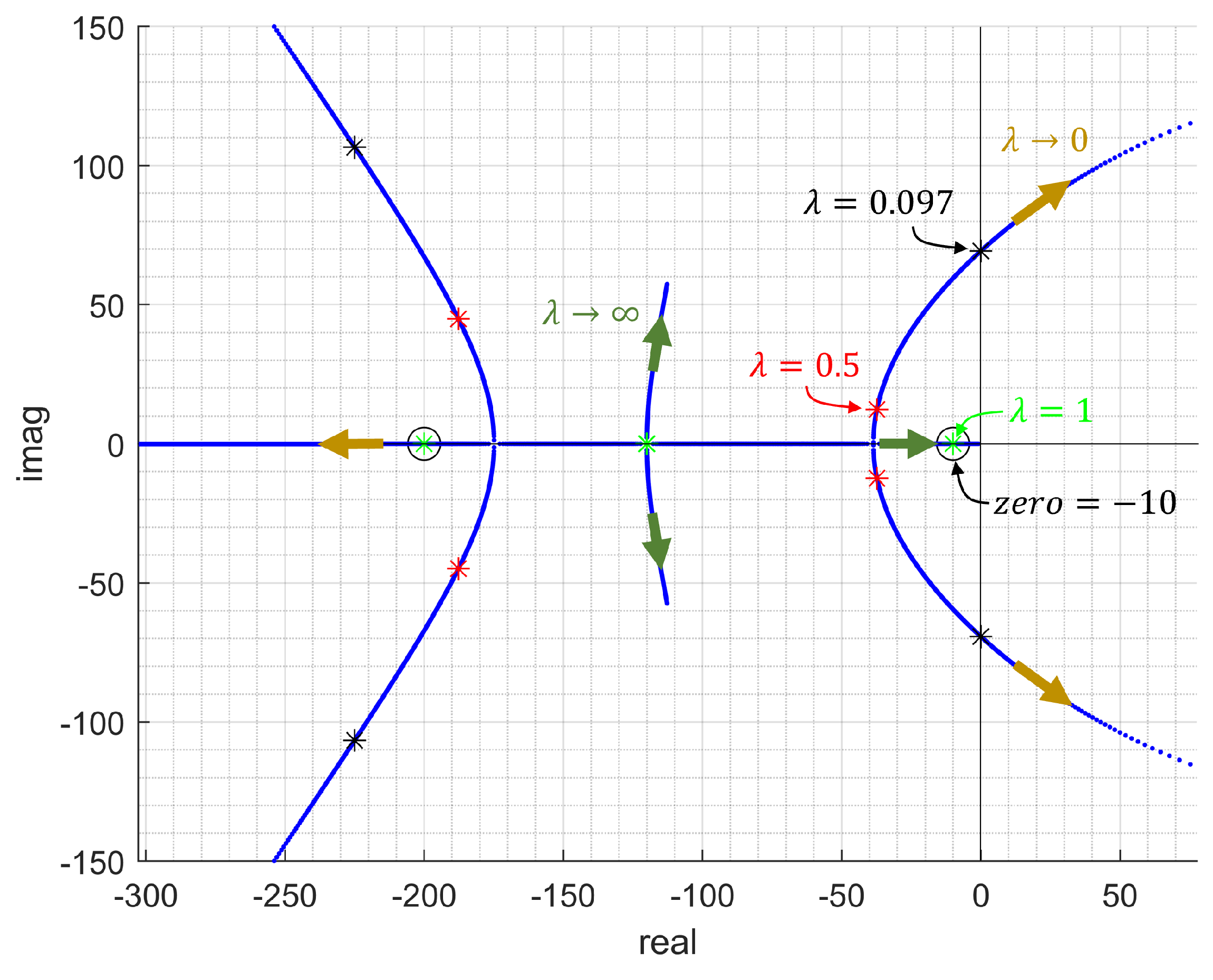
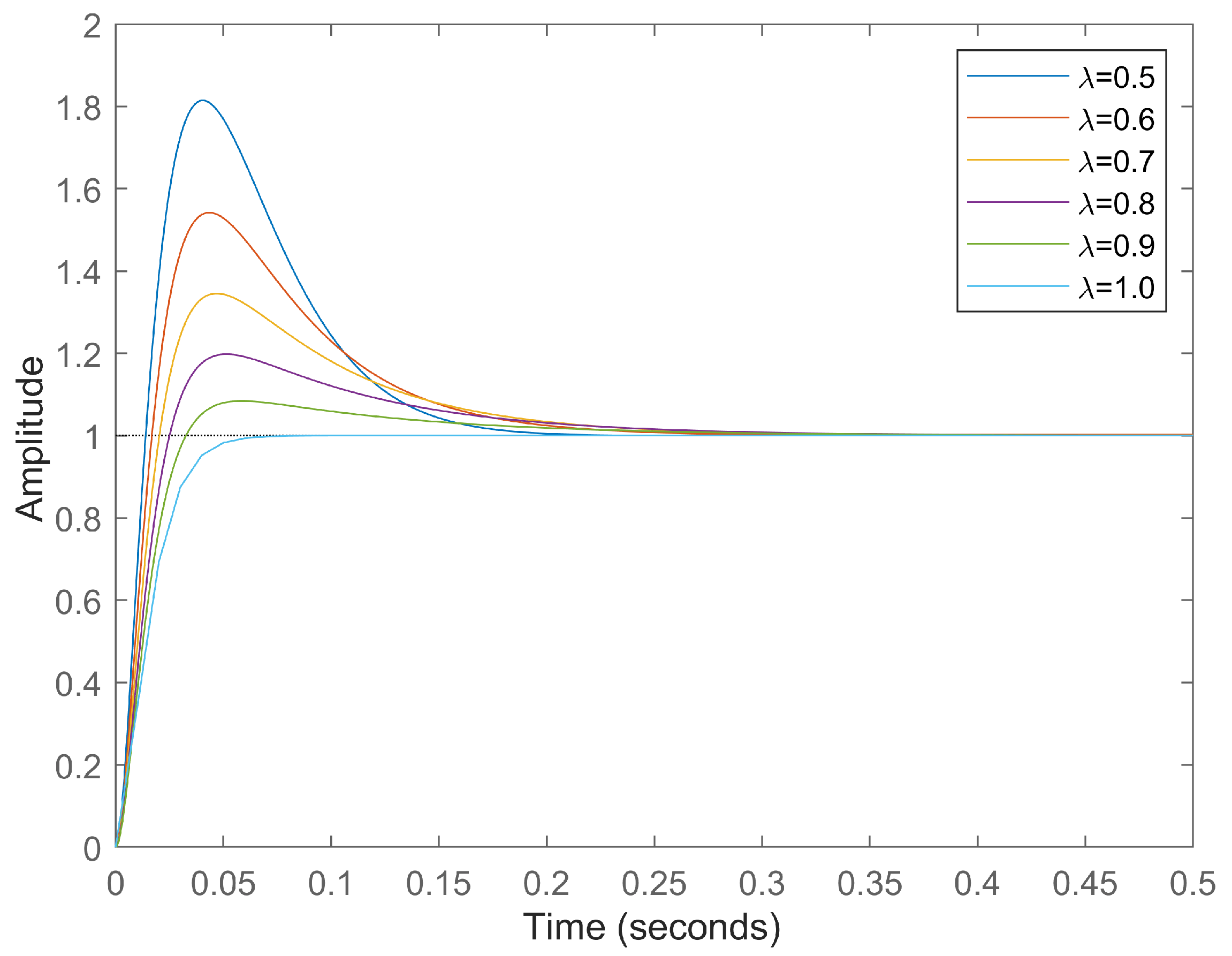
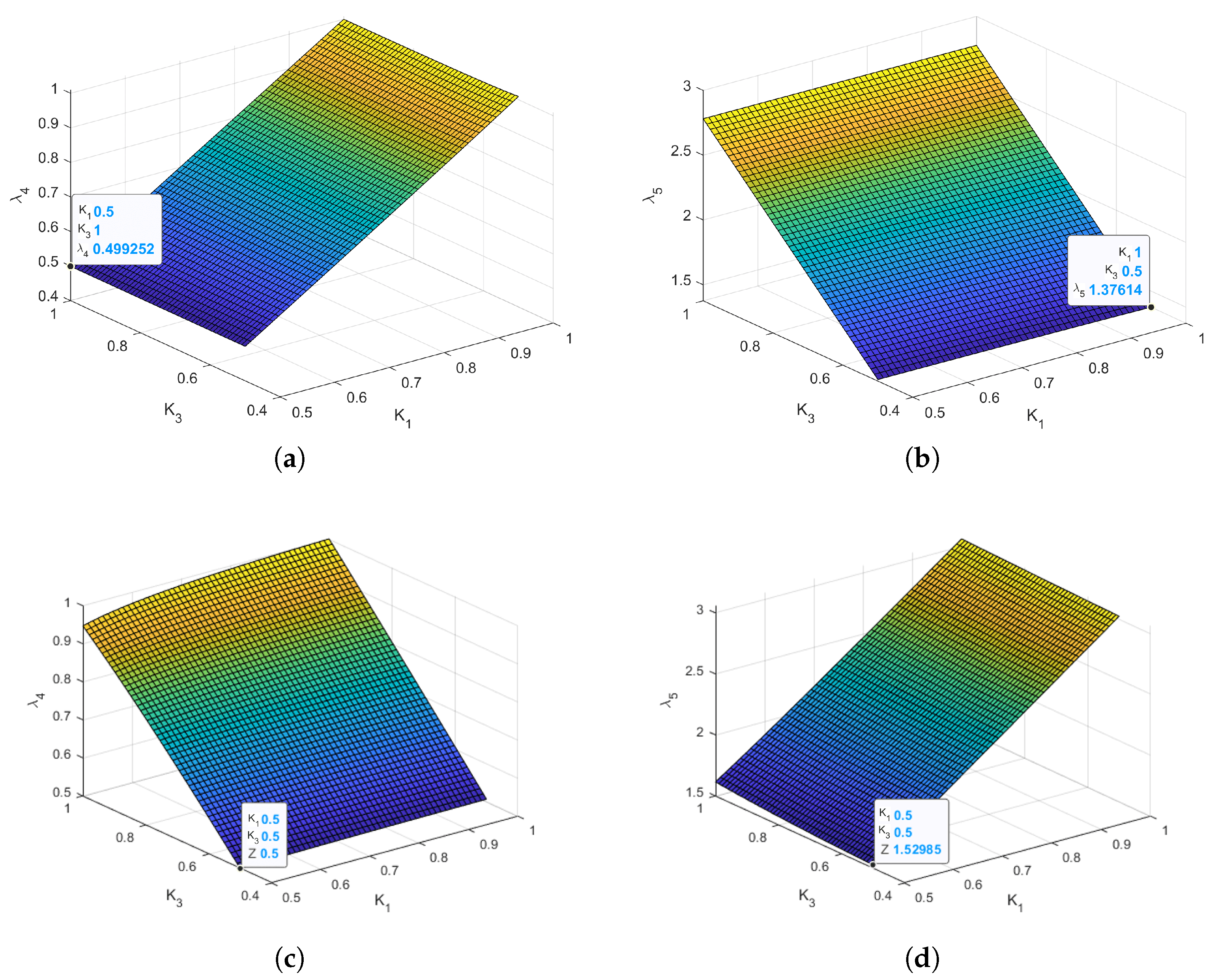
3.2. Bounds on K to Ensure Stability with Control Performance Considerations

In the previous subsection, it was shown that the stability margin regarding control effectiveness uncertainty is significantly relaxed by accounting for the actuator dynamics, sampling time delay, and low-pass filters. However, it was also observed that control performance may degrade as $\lambda$ approaches the imaginary axis, leading to a reduction in the damping ratio. This degradation was further amplified by the low-pass filter, which introduces a zero at −10 in Figure 5, causing exaggerated overshoots. Thus, it is preferable to set a minimum desired value for $\lambda$ to maintain effective control performance of the INDI controller.

To select this minimum $\lambda$, the step response at various values of $\lambda$ was examined. As shown in Figure 6, the minimum $\lambda$ was chosen to be approximately 0.5 (${\lambda }_{\min }\approx 0.5$) based on the overshoot characteristics of the transfer function $H\left(s\right)$ in Equation (13). It is important to note that the step responses exhibited greater overshoot than expected based on the pole locations due to the effect of the zero located at −10, which is relatively close to the origin and amplifies the transient response.

Next, based on the desired minimum $\lambda$, the lower bound of the components of the K matrix in Equation (3) can be determined. For the proposed control effectiveness matrix, the square matrix $\widehat{G}{G}^{-1}$ is formulated as shown in Equation (14) by using Equation (4):

$$\widehat{G}{G}^{-1}=K·G_{I_{\mathrm{UAM}}}^{-1}·G_{C_{\mathrm{UAM}}}·G_{C_{\mathrm{UAM}\&o}}^{-1}·G_{I_{\mathrm{UAM}\&o}}=K·\mathsf{\Xi }$$

(14)

where $G=G_{I_{\mathrm{UAM}\&o}}^{-1}·G_{C_{\mathrm{UAM}\&o}}$ is the control effectiveness matrix comprising the true geometric and inertial parameters of the UAM and the object in the gripper ($\mathrm{UAM}\&o$). To simplify the eigenvalue analysis of the given UAM, the center of mass of the picked-up object is constrained to lie along the UAM’s longitudinal plane (Figure 2), thereby preserving symmetry with respect to this plane while the object is being held. For convenience, $G_{I_{\mathrm{UAM}}}^{-1}·G_{C_{\mathrm{UAM}}}·G_{C_{\mathrm{UAM}\&o}}^{-1}·G_{I_{\mathrm{UAM}\&o}}$ is represented as $\mathsf{\Xi }$.

It is important to note that, for the given UAM, the square matrix $\widehat{G}{G}^{-1}$, Equation (14), always has positive real eigenvalues with zero imaginary components. This holds true because $\mathsf{\Xi }$ has positive real eigenvalues with no imaginary components, as illustrated in Equation (15), where

$$\mathsf{\Pi }={\displaystyle \frac{K_{T_1}sin\gamma \left(K_{Q_1}d{r}_{of{f}_x}-K_{T_1}{r}_{p_{1_y}}d{r}_{of{f}_z}\right)}{K_{Q_1}^{2}cos\gamma +K_{T_1}^2{r}_{p_{1_y}}^{2}cos\gamma -K_{Q_1}{K}_{T_1}sin\gamma \left(r_{p_{1_x}}-r_{of{f}_{x_{\mathrm{UAM}\&o}}}\right)+K_{T_1}^2{r}_{p_{1_y}}sin\gamma \left(r_{p_{1_z}}-r_{of{f}_{z_{\mathrm{UAM}\&o}}}\right)}}$$

and $K_{T_i}$ and $K_{Q_i}$ represent the propeller thrust and torque coefficients. Multiplying the $\mathsf{\Xi }$ matrix by the positive real diagonal matrix K ensures that the eigenvalues remain positive real with no imaginary components. The eigenvalues of the $\mathsf{\Xi }$ matrix are given as Equation (15):

$$\begin{array}{cc}\hfill {\lambda }_{{\mathsf{\Xi }}_1}& =\left(1+\mathsf{\Pi }\right)\left\{1+m_{\mathrm{UAM}}·\left(1+{\displaystyle \frac{m_{\mathrm{UAM}}}{m_o}}\right)·\left({\displaystyle \frac{I_{{\mathrm{UAM}}_{xx}}d{r}_{of{f}_x}^2+I_{{\mathrm{UAM}}_{zz}}d{r}_{of{f}_z}^2+2I_{{\mathrm{UAM}}_{xz}}d{r}_{of{f}_x}d{r}_{of{f}_z}}{I_{{\mathrm{UAM}}_{xx}}{I}_{{\mathrm{UAM}}_{zz}}-I_{{\mathrm{UAM}}_{xz}}^2}}\right)\right\}\hfill \\ \hfill {\lambda }_{{\mathsf{\Xi }}_2}& =1\hfill \\ \hfill {\lambda }_{{\mathsf{\Xi }}_3}& =1+m_{\mathrm{UAM}}·\left(1+{\displaystyle \frac{m_{\mathrm{UAM}}}{m_o}}\right)\left({\displaystyle \frac{d{r}_{of{f}_x}^2+d{r}_{of{f}_z}^2}{I_{{\mathrm{UAM}}_{yy}}}}\right)\hfill \\ \hfill {\lambda }_{{\mathsf{\Xi }}_4}& =1+{\displaystyle \frac{m_o}{m_{\mathrm{UAM}}}}\hfill \\ \hfill {\lambda }_{{\mathsf{\Xi }}_5}& =1+{\displaystyle \frac{m_o}{m_{\mathrm{UAM}}}}\hfill \end{array}$$

(15)

The term $d{r}_{off}$ in Equation (15) denotes the shift in the center of mass that occurs when an object is grasped or added to the UAM. Among the five obtained eigenvalues, the four eigenvalues from ${\lambda }_{{\mathsf{\Xi }}_2}$ to ${\lambda }_{{\mathsf{\Xi }}_5}$ are real and greater than or equal to 1, with zero imaginary components. This is because the analytic terms in ${\lambda }_{{\mathsf{\Xi }}_{3\sim 5}}$, as shown in Equation (15), apart from the constant value of 1, are non-negative. These non-negative analytic terms reduce to zero when the object’s mass, $m_o$, is zero. To evaluate the first eigenvalue of the $\mathsf{\Xi }$ matrix, ${\lambda }_{{\mathsf{\Xi }}_1}$, it is expressed differently as per Equation (16):

$${\lambda }_{{\mathsf{\Xi }}_1}=\left(1+\mathsf{\Pi }\right)\left\{1+m_{\mathrm{UAM}}·\left(1+{\displaystyle \frac{m_{\mathrm{UAM}}}{m_o}}\right)·{\displaystyle \frac{\left[\begin{array}{cc}d{r}_{of{f}_x}& d{r}_{of{f}_z}\end{array}\right]\left[\begin{array}{cc}{I}_{{\mathrm{UAM}}_{xx}}& I_{{\mathrm{UAM}}_{xz}}\\ I_{{\mathrm{UAM}}_{xz}}& I_{{\mathrm{UAM}}_{zz}}\end{array}\right]\left[\begin{array}{c}d{r}_{of{f}_x}\\ d{r}_{of{f}_z}\end{array}\right]}{I_{{\mathrm{UAM}}_{xx}}{I}_{{\mathrm{UAM}}_{zz}}-I_{{\mathrm{UAM}}_{xz}}^2}}\right\}$$

(16)

The right-hand term in braces in Equation (16) always has a real value greater than or equal to 1. The denominator in the rightmost fraction represents the determinant of the inertia tensor in the $\widehat{x}-\widehat{z}$ plane, which is always greater than 0, as the UAM is assumed to be a rigid body. In turn, since all leading principal minors of the inertia tensor matrix in the $\widehat{x}-\widehat{z}$ plane are positive according to Sylvester’s criterion [36], the numerator term in Equation (16) is positive definite. The left parenthesis term ($1+\mathsf{\Pi }$) is also positive real when considering the actual UAM parameters. Therefore, ${\lambda }_{{\mathsf{\Xi }}_1}$ is real and positive, with no imaginary part.

The eigenvalues of the $\mathsf{\Xi }$ matrix have been shown to be positive and real, with no imaginary components. Similarly, the eigenvalues of the $\widehat{G}{G}^{-1}$ matrix, which are also positive and real with no imaginary components, will now be derived analytically following the approach used for the $\mathsf{\Xi }$ matrix. This derivation enables the determination of the lower bounds for the components of the K matrix in Equation (3). Among the five positive real eigenvalues of the square matrix $\widehat{G}{G}^{-1}$, three eigenvalues (${\lambda }_1$ to ${\lambda }_3$) can be expressed analytically in terms of the moment of inertia in the $\widehat{y}$ direction, the total mass, and the parameters $K_2$ and $K_4$, as presented in Equation (17):

$$\begin{array}{cc}\hfill {\lambda }_1& =K_2{\displaystyle \frac{I_{\mathrm{UAM}\&o_{yy}}}{I_{{\mathrm{UAM}}_{yy}}}}\hfill \\ \hfill {\lambda }_2& ={\lambda }_3=K_4{\displaystyle \frac{m_{\mathrm{UAM}\&o}}{m_{\mathrm{UAM}}}}\hfill \end{array}$$

(17)

The remaining two eigenvalues of $\widehat{G}{G}^{-1}$ (${\lambda }_4$ and ${\lambda }_5$) are expressed as functions of the moment of inertia in the $\widehat{x}$ and $\widehat{z}$ directions, the product of inertia in the $\widehat{x}-\widehat{z}$ plane, and $K_1$ and $K_3$. Due to the length of the full set of eigenvalues and space constraints, they are not included in this paper; however, Equation (18) offers a general representation of these eigenvalues:

$$\begin{array}{c}\hfill {\lambda }_4={\lambda }_5=f(I_{{\mathrm{UAM}}_{xx}},I_{\mathrm{UAM}\&o_{xx}},I_{{\mathrm{UAM}}_{yy}},I_{\mathrm{UAM}\&o_{yy}},I_{{\mathrm{UAM}}_{xz}},I_{\mathrm{UAM}\&o_{xz}},K_1,K_3)\end{array}$$

(18)

Since $K_2$ and $K_4$ are related only to ${\lambda }_1$, ${\lambda }_2$, and ${\lambda }_3$, the bounds of $K_2$ and $K_4$ can be determined from these three eigenvalues while considering that the desired minimum eigenvalue must be ${\lambda }_{\min }\approx 0.5$. As the UAM picks up an object, the moment of inertia in its $\widehat{y}$ direction ($I_{{\mathrm{UAM}}_{yy}}$) and the mass ($m_{\mathrm{UAM}}$) increase, meaning that $I_{\mathrm{UAM}\&o_{yy}}/I_{{\mathrm{UAM}}_{yy}}$ and $m_{\mathrm{UAM}\&o}/m_{\mathrm{UAM}}$ are always greater than or equal to 1 (equal to 1 when the UAM has no object). Therefore, by setting the lower bounds of both $K_2$ and $K_4$ to 0.5, ${\lambda }_1$, ${\lambda }_2$, and ${\lambda }_3$ remain greater than or equal to 0.5.

Due to the analytical complexity, the lower bounds of $K_1$ and $K_3$ were determined numerically by considering the lower bounds of ${\lambda }_4$ and ${\lambda }_5$. Figure 7 presents the numerical values of ${\lambda }_4$ and ${\lambda }_5$ with respect to $K_1$ and $K_3$ for specific cases where the manipulator is either stretched forward ($q_1={80}^{\circ }$, $q_2=q_3={10}^{\circ }$; see Figure 7a,b) or curled ($q_1=-{60}^{\circ }$, $q_2={60}^{\circ }$, $q_3={60}^{\circ }$; see Figure 7c,d), representing typical grasp-and-hold maneuvers. In both scenarios, the manipulator holds a 2 kg object, with the minimum bound of K set to 0.5.

In Figure 7a,c, it can be observed that the eigenvalue ${\lambda }_4$ falls slightly below 0.5 for the stretched arm configuration and reaches exactly 0.5 for the curled arm configuration when the difference between $K_1$ and $K_3$ is maximized. Additionally, Figure 7b,d show that ${\lambda }_5$ consistently remains greater than ${\lambda }_4$. Through a numerical analysis of ${\lambda }_4$ and ${\lambda }_5$ across all possible configurations and object mass weights, the lower bounds of $K_1$ and $K_3$ are set to 0.5 to ensure that the minimum eigenvalues of ${\lambda }_4$ and ${\lambda }_5$ remain close to 0.5. This is a loose constraint; however, the stability of the INDI controller in terms of control effectiveness uncertainty is still ensured, as a sufficient margin exists for the eigenvalues (from 0.5 to 0.1), and control performance degradation is prevented by maintaining the minimum eigenvalues of ${\lambda }_4$ and ${\lambda }_5$ close to 0.5.

As illustrated in Figure 5, the dominant pole moves closer to the imaginary axis as $\lambda$ increases, resulting in a reduced natural frequency and degraded control performance for the transfer function $H\left(s\right)$. Thus, it is preferable to establish an upper bound for K to keep the eigenvalues of $\widehat{G}{G}^{-1}$ within limits. To determine this upper bound for K, an inertial property of the UAM is utilized. In Equation (3), ${\widehat{G}}_I$ ideally represents the matrix composed of the inertia parameters of the UAM, including an object in the gripper, if present. The maximum K values are chosen based on the principle that adding an object increases the inertia parameters (the moment of inertia and total mass) of the UAM system compared to those of the UAM without the object, as shown in Equation (19):

$$\begin{array}{cc}\hfill & {\widehat{I}}_{xx}={\displaystyle \frac{I_{{\mathrm{UAM}}_{xx}}}{K_1}}\ge I_{{\mathrm{UAM}}_{xx}}\hfill \\ \hfill & {\widehat{I}}_{yy}={\displaystyle \frac{I_{{\mathrm{UAM}}_{yy}}}{K_2}}\ge I_{{\mathrm{UAM}}_{yy}}\hfill \\ \hfill & {\widehat{I}}_{zz}={\displaystyle \frac{I_{{\mathrm{UAM}}_{zz}}}{K_3}}\ge I_{{\mathrm{UAM}}_{zz}}\hfill \\ \hfill & \widehat{m}={\displaystyle \frac{m_{\mathrm{UAM}}}{K_4}}\ge m_{\mathrm{UAM}}\hfill \end{array}$$

(19)

Utilizing the inequality relations in Equation (19), the maximum values of $K_1$, $K_2$, $K_3$, and $K_4$ are determined to be 1. Therefore, the bounds for K are defined as shown in Equation (20):

$$0.5\le K_i\le 1,\mathrm{where}i=1,2,3,4$$

(20)

3.3. Constrained Kalman Filter

In this subsection, the estimation procedure for ${\widehat{G}}_I$ is described. The bounds of the weighting factor K were defined, as shown in Equation (20), to ensure the stability of the INDI controller under control effectiveness matrix uncertainty while maintaining control performance. Based on these defined bounds, the limits of the ${\widehat{G}}_I$ components—representing a combination of the weighting factor K and the inertia parameters of the UAM without the object—can be established as shown in Equation (21):

$$\begin{array}{cc}\hfill & I_{{\mathrm{UAM}}_{xx}}\le {\displaystyle \frac{I_{{\mathrm{UAM}}_{xx}}}{K_1}}={\widehat{I}}_{xx}\le 2·I_{{\mathrm{UAM}}_{xx}}\hfill \\ \hfill & I_{{\mathrm{UAM}}_{yy}}\le {\displaystyle \frac{I_{{\mathrm{UAM}}_{yy}}}{K_2}}={\widehat{I}}_{yy}\le 2·I_{{\mathrm{UAM}}_{yy}}\hfill \\ \hfill & I_{{\mathrm{UAM}}_{zz}}\le {\displaystyle \frac{I_{{\mathrm{UAM}}_{zz}}}{K_3}}={\widehat{I}}_{zz}\le 2·I_{{\mathrm{UAM}}_{zz}}\hfill \\ \hfill & m_{\mathrm{UAM}}\le {\displaystyle \frac{m_{\mathrm{UAM}}}{K_4}}=\widehat{m}\le 2·m_{\mathrm{UAM}}\hfill \end{array}$$

(21)

The components of ${\widehat{G}}_I$ in Equation (4) will be estimated by considering the maneuvers of both the UAV and the manipulator while satisfying the inequality conditions in Equation (21). Since the estimation variables must adhere to these inequality constraints (Equation (21)), a constrained Kalman filter is used in this research, which applies a quadratic programming step after the correction stage in the Kalman filter estimation process [37]. Similar to the approaches in [30], this estimation process leverages the relationship between the control input measurements and the accelerations of both the UAV and the manipulator. The estimation variables include the moments of inertia (${\widehat{I}}_{xx},{\widehat{I}}_{yy},{\widehat{I}}_{zz}$) and the total mass ($\widehat{m}$). Similar to traditional Kalman filters, the proposed approach employs two models for variable estimation: (i) a motion model and (ii) a measurement model.

The motion model equations for inertia estimation are given in Equation (22):

$$\begin{array}{cc}\hfill {\dot{I}}_{{\mathrm{UAM}}_{xx}}& ={\dot{I}}_{{\mathrm{UAM}}_{11}}^{\prime }+{\epsilon }_{xx}\hfill \\ \hfill {\dot{I}}_{{\mathrm{UAM}}_{yy}}& ={\dot{I}}_{{\mathrm{UAM}}_{22}}^{\prime }+{\epsilon }_{yy}\hfill \\ \hfill {\dot{I}}_{{\mathrm{UAM}}_{zz}}& ={\dot{I}}_{{\mathrm{UAM}}_{33}}^{\prime }+{\epsilon }_{zz}\hfill \\ \hfill {\dot{m}}_{\mathrm{UAM}}& ={\epsilon }_m\hfill \end{array}$$

(22)

where ${\dot{I}}_{\mathrm{UAM}}^{\prime }$ represents the time derivatives of the UAM moment of inertia tensor components, and $\epsilon$ denotes Gaussian noise for each motion component. ${\dot{I}}_{\mathrm{UAM}}^{\prime }$ is obtained using measurements of the arm joint positions and velocities, along with the inertia parameters of the UAM without the object, as described in [8]. Given the model uncertainty due to unknown object inertia and sensor noise, Gaussian noise is incorporated into the motion models. The motion model for the total mass ($\widehat{m}$) is represented as a simple random walk model [38].

For the measurement models, the relationship between the control input increments and the acceleration increments in Equation (23) is used, with Gaussian noise, $\nu$, added to account for measurement uncertainty:

$$\Delta U=G_{C_{\mathrm{UAM}}}^{-1}·{\widehat{G}}_I·\Delta Ac{c}_m+\nu$$

(23)

where

$$\begin{array}{cc}\hfill & \Delta Ac{c}_m=\Delta Ac{c}_{\mathrm{UAV}}+\Delta Ac{c}_{\mathrm{ARM}}\hfill \\ \hfill & \Delta Ac{c}_{\mathrm{UAV}}={\left[\begin{array}{ccccc}\Delta P& \Delta Q& \Delta R& \Delta a_x^P& \Delta a_z^P\end{array}\right]}^T\hfill \\ \hfill & \Delta Ac{c}_{\mathrm{ARM}}=[0;0;0;\Delta {\displaystyle \frac{d^2}{d{t}^2}}\left(q_1\right)\times {}_1\overrightarrow{r}_{{\mathrm{CoM}}_{1\sim o}}+\Delta {\displaystyle \frac{d^2}{d{t}^2}}\left(q_2\right)\times {}_2\overrightarrow{r}_{{\mathrm{CoM}}_{2\sim o}}+\Delta {\displaystyle \frac{d^2}{d{t}^2}}\left(q_3\right)\times {}_3\overrightarrow{r}_{{\mathrm{CoM}}_{3\sim o}}]\hfill \end{array}$$

The acceleration increments ($\Delta Ac{c}_m$) incorporate both the acceleration from the arm movement ($\Delta Ac{c}_{ARM}$) and the UAV acceleration ($\Delta Ac{c}_{UAV}$) to account for the reaction forces generated by the arm’s motion. In Equation (23), ${}_j\overrightarrow{r}_{{\mathrm{CoM}}_{i\sim o}}$, where $j=1,2,3$ and $i=1,2,3$, is the position vector from the jth joint to the position of the center of mass of the combination from the ith link onward to the object. Details about Equation (23) can be found in [30]. Gaussian noises are added to account for the inertia mismatch and the sensor measurements. It should be noted that ${\widehat{I}}_{xz}$ and ${\widehat{I}}_{zx}$ in ${\widehat{G}}_I$ can be reformulated as ${\widehat{I}}_{zz}·{\displaystyle \frac{I_{{\mathrm{UAM}}_{xz}}}{I_{{\mathrm{UAM}}_{zz}}}}$ and ${\widehat{I}}_{xx}·{\displaystyle \frac{I_{{\mathrm{UAM}}_{xz}}}{I_{{\mathrm{UAM}}_{xx}}}}$, respectively, since ${\widehat{I}}_{xz}$ contains the weighting factor $K_3$, and ${\widehat{I}}_{zx}$ contains the weighting factor $K_1$, as shown in Equation (4), which is determined by the estimation of ${\widehat{I}}_{xx}$ and ${\widehat{I}}_{zz}$. Therefore, Equation (23) can be reformulated as Equation (24):

$$\begin{array}{cc}\hfill \Delta U_1& ={\widehat{I}}_{xx}\Delta Ac{c}_{m_1}\left(G_{C_{{\mathrm{UAM}}_{11}}}^{-1}+G_{C_{{\mathrm{UAM}}_{13}}}^{-1}{\displaystyle \frac{I_{{\mathrm{UAM}}_{xz}}}{I_{{\mathrm{UAM}}_{xx}}}}\right)+{\widehat{I}}_{yy}\Delta Ac{c}_{m_2}{G}_{C_{{\mathrm{UAM}}_{12}}}^{-1}\hfill \\ \hfill & +{\widehat{I}}_{zz}\Delta Ac{c}_{m_3}\left(G_{C_{{\mathrm{UAM}}_{13}}}^{-1}+G_{C_{{\mathrm{UAM}}_{11}}}^{-1}{\displaystyle \frac{I_{{\mathrm{UAM}}_{xz}}}{I_{{\mathrm{UAM}}_{zz}}}}\right)+m_{\mathrm{UAM}}\left(\Delta Ac{c}_{m_4}{G}_{C_{{\mathrm{UAM}}_{14}}}^{-1}+\Delta Ac{c}_{m_5}{G}_{C_{{\mathrm{UAM}}_{15}}}^{-1}\right)+{\nu }_1\hfill \\ \hfill \Delta U_2& ={\widehat{I}}_{xx}\Delta Ac{c}_{m_1}\left(G_{C_{{\mathrm{UAM}}_{21}}}^{-1}+G_{C_{{\mathrm{UAM}}_{23}}}^{-1}{\displaystyle \frac{I_{{\mathrm{UAM}}_{xz}}}{I_{{\mathrm{UAM}}_{xx}}}}\right)+{\widehat{I}}_{yy}\Delta Ac{c}_{m_2}{G}_{C_{{\mathrm{UAM}}_{22}}}^{-1}\hfill \\ \hfill & +{\widehat{I}}_{zz}\Delta Ac{c}_{m_3}\left(G_{C_{{\mathrm{UAM}}_{23}}}^{-1}+G_{C_{{\mathrm{UAM}}_{21}}}^{-1}{\displaystyle \frac{I_{{\mathrm{UAM}}_{xz}}}{I_{{\mathrm{UAM}}_{zz}}}}\right)+m_{\mathrm{UAM}}\left(\Delta Ac{c}_{m_4}{G}_{C_{{\mathrm{UAM}}_{24}}}^{-1}+\Delta Ac{c}_{m_5}{G}_{C_{{\mathrm{UAM}}_{25}}}^{-1}\right)+{\nu }_2\hfill \\ \hfill \Delta U_3& =-{\widehat{I}}_{xx}\Delta Ac{c}_{m_1}\left(G_{C_{{\mathrm{UAM}}_{11}}}^{-1}+G_{C_{{\mathrm{UAM}}_{13}}}^{-1}{\displaystyle \frac{I_{{\mathrm{UAM}}_{xz}}}{I_{{\mathrm{UAM}}_{xx}}}}\right)+{\widehat{I}}_{yy}\Delta Ac{c}_{m_2}{G}_{C_{{\mathrm{UAM}}_{12}}}^{-1}\hfill \\ \hfill & -{\widehat{I}}_{zz}\Delta Ac{c}_{m_3}\left(G_{C_{{\mathrm{UAM}}_{13}}}^{-1}+G_{C_{{\mathrm{UAM}}_{11}}}^{-1}{\displaystyle \frac{I_{{\mathrm{UAM}}_{xz}}}{I_{{\mathrm{UAM}}_{zz}}}}\right)+m_{\mathrm{UAM}}\left(\Delta Ac{c}_{m_4}{G}_{C_{{\mathrm{UAM}}_{34}}}^{-1}+\Delta Ac{c}_{m_5}{G}_{C_{{\mathrm{UAM}}_{35}}}^{-1}\right)+{\nu }_3\hfill \\ \hfill \Delta U_4& =-{\widehat{I}}_{xx}\Delta Ac{c}_{m_1}\left(G_{C_{{\mathrm{UAM}}_{21}}}^{-1}+G_{C_{{\mathrm{UAM}}_{23}}}^{-1}{\displaystyle \frac{I_{{\mathrm{UAM}}_{xz}}}{I_{{\mathrm{UAM}}_{xx}}}}\right)-{\widehat{I}}_{yy}\Delta Ac{c}_{m_2}{G}_{C_{{\mathrm{UAM}}_{22}}}^{-1}\hfill \\ \hfill & -{\widehat{I}}_{zz}\Delta Ac{c}_{m_3}\left(G_{C_{{\mathrm{UAM}}_{23}}}^{-1}+G_{C_{{\mathrm{UAM}}_{21}}}^{-1}{\displaystyle \frac{I_{{\mathrm{UAM}}_{xz}}}{I_{{\mathrm{UAM}}_{zz}}}}\right)+m_{\mathrm{UAM}}\left(\Delta Ac{c}_{m_4}{G}_{C_{{\mathrm{UAM}}_{44}}}^{-1}+\Delta Ac{c}_{m_5}{G}_{C_{{\mathrm{UAM}}_{45}}}^{-1}\right)+{\nu }_4\hfill \\ \hfill \Delta U_5& ={\widehat{I}}_{yy}\Delta Ac{c}_{m_2}{G}_{C_{{\mathrm{UAM}}_{52}}}^{-1}+m_{\mathrm{UAM}}\left(\Delta Ac{c}_{m_4}{G}_{C_{{\mathrm{UAM}}_{54}}}^{-1}+\Delta Ac{c}_{m_5}{G}_{C_{{\mathrm{UAM}}_{55}}}^{-1}\right)+{\nu }_5\hfill \end{array}$$

(24)

Using the motion and measurement models (Equations (22) and (24), respectively), along with the inequality condition (Equation (21)), a constrained Kalman filter is formulated within the adaptive law to estimate the components of the inertia matrix (${\widehat{G}}_I$) based on the approach in [37]. The estimated inertia matrix will be used to formulate the necessary control increment, as shown in Equation (5).

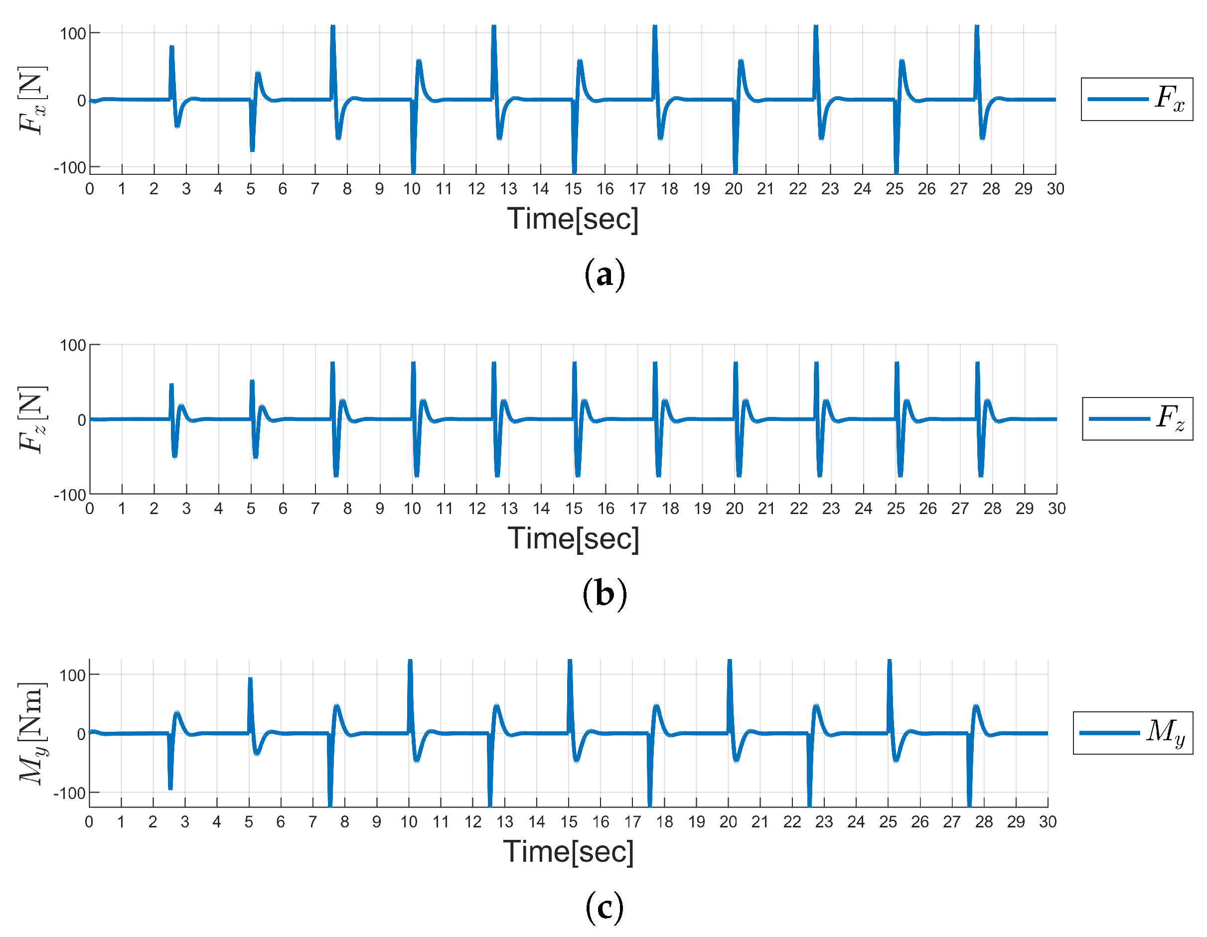
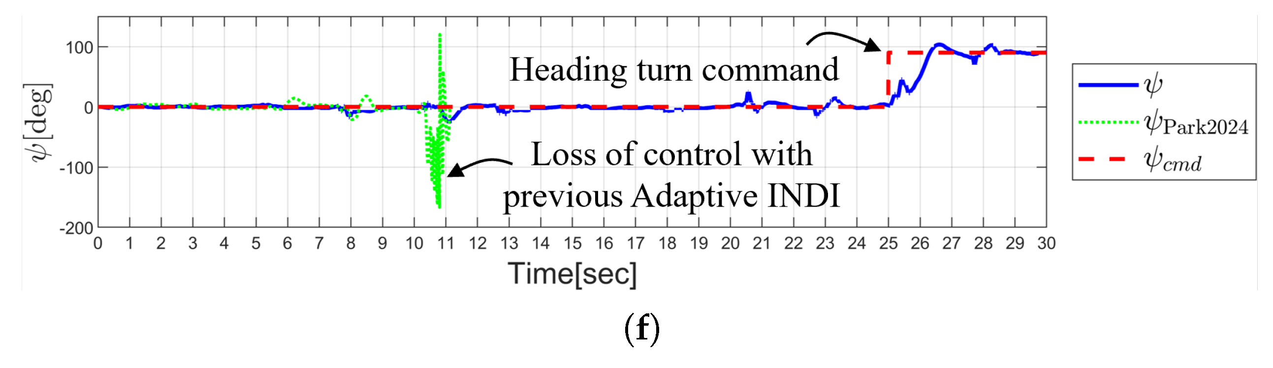
4. Simulation Results

The proposed adaptive INDI control methodology was analyzed to validate its stability and performance advantages over previously developed UAM controllers, particularly in scenarios involving rapid arm movements while holding objects with varying mass. To achieve this, a simulation test using a multi-step command scenario was conducted, similar to that in [30]. During the simulation, the UAV followed a series of step-input trajectory commands of ENU positions ($p{E}_{cmd}$, $p{N}_{cmd}$, and $p{U}_{cmd}$) and pitch and yaw attitude (${\theta }_{cmd}$, ${\psi }_{cmd}$) as per Equation (25), while the robot arm moved swiftly back and forth between Pose 1 and Pose 2 every 2.5 s as per Equation (26), as illustrated in Figure 8 and Figure 9.

$$\begin{array}{cc}\hfill & p{E}_{cmd}=2u(t-5)\mathrm{m}\hfill \\ \hfill & p{N}_{cmd}=2u(t-10)\mathrm{m}\hfill \\ \hfill & p{U}_{cmd}=2(u(t-15)+1)\mathrm{m}\hfill \\ \hfill & {\theta }_{cmd}=-45u(t-20)deg\hfill \\ \hfill & {\psi }_{cmd}=90u(t-25)deg\hfill \\ \hfill & \mathrm{where}u\left(t\right)=\left\{\begin{array}{c}0,t<0\\ 1,t\ge 0\end{array}\right.\hfill \end{array}$$

(25)

$$q_{1_{cmd}}=q_{2_{cmd}}=q_{3_{cmd}}=20\left(1+\sum _{k=1}^{\infty }{(-1)}^{k}2u(t-2.5k)\right)deg$$

(26)

The size and inertia parameters of each component of the UAM utilized in the simulation tests are detailed in

Table 1. Size and inertia parameters of the UAM components.

	Size [m]	Mass [kg]	${\mathit{I}}_{\mathbf{xx}}$ [$\mathbf{kg}\mathit{·}{\mathbf{m}}^2$]	${\mathit{I}}_{\mathbf{yy}}$ [$\mathbf{kg}\mathit{·}{\mathbf{m}}^2$]	${\mathit{I}}_{\mathbf{zz}}$ [$\mathbf{kg}\mathit{·}{\mathbf{m}}^2$]	${\mathit{I}}_{\mathbf{xz}}$ [$\mathbf{kg}\mathit{·}{\mathbf{m}}^2$]	${\mathit{I}}_{\mathbf{xy}}$ [$\mathbf{kg}\mathit{·}{\mathbf{m}}^2$]	${\mathit{I}}_{\mathbf{yz}}$ [$\mathbf{kg}\mathit{·}{\mathbf{m}}^2$]
Navig8-UAV	Length: 1.0 Width: 0.8 Height: 0.2	5.0	0.0667	0.1492	0.2019	0.0147	0	0
Each arm linkage	Length: 0.3	0.5	0.0037	0.0037	0	0	0	0
Object (Sphere)	Radius: 0.05	1→2	0.001	0.001	0.001	0	0	0

.

Compared to the previous simulation [30], the mass of the object held by the gripper was increased from 1 kg to 2 kg during the simulation, and the manipulator’s range of motion was expanded. These adjustments were made to produce greater reaction forces and torques on the UAV, thereby providing a more rigorous test of the controller’s capabilities. The arm movement generated significant reaction forces and torques on the UAV, as illustrated in Figure 10, along with high joint angular velocities and accelerations, as shown in Figure 11.

The maximum angular velocity and acceleration of the joints were recorded at 4.0 rad/s and 42 rad/${\mathrm{s}}^2$, respectively, while the peak reaction force and torque from the arm movement on the UAM reached 130.7 N and 125.8 Nm, respectively.

The proposed controller was implemented using the same outer-loop control structure described in [29]. To simulate the noisy characteristics of real-world sensors, the position and velocity of the three arm joints ($q_1$, $q_2$, and $q_3$) were assumed to have noise with standard deviations of 0.08 rad and 0.01 rad/s. Joint accelerations were obtained by differentiating the measured angular velocities. For the UAV, the sensor noise standard deviations were set as follows: 0.01 rad/s for the angular velocity, 0.5 m/${\mathrm{s}}^2$ for the linear acceleration, 20 rad/s for the propeller angular speed, and 0.08 rad for the duct tilt angle measurements. The angular acceleration of the UAV was calculated by differentiating the angular velocity measurements directly.

Given the sensor noise levels, the Kalman filter’s noise covariance was set to $[{1500}^2$, ${2000}^2$, ${1500}^2$, ${2000}^2$, ${10,000}^2]$ for each measurement model equation. For each motion model involving the moment of inertia tensor components and the mass motion, the covariance values were set to $[{10}^{-4}$, $5·{10}^{-5}$, ${10}^{-4}$, $5·{10}^{-4}]$. The time constant for the low-pass filters in the adaptive law was set to 0.7 s, while the low-pass filter for INDI control acceleration feedback was set to 0.1 s. These values were determined through a process of trial and error.

Figure 12 shows the UAV’s position ($pE$, $pN$, and $pU$) and attitude angles ($\varphi$, $\theta$, and $\psi$) during the simulation.

The solid blue lines represent the actual UAV states controlled by the proposed adaptive INDI controller, the dotted green line indicates the UAV states controlled by the adaptive INDI controller reported in [30], and the dashed red lines represent the commands applied to the UAV. Furthermore, Figure 13 displays the UAV’s acceleration states ($\dot{P}$, $\dot{Q}$, $\dot{R}$, $a_x^P$, $a_y^P$, and $a_z^P$) under the control of the proposed adaptive controller.

Figure 14 shows the actuator inputs (duct tilt angles and propeller angular speeds) during the simulation.

Figure 15 shows the results of the ${\widehat{G}}_I$ matrix estimation process, where the solid blue line represents the estimated values, the dashed red line represents the true inertia parameters of the UAM with an object, and the dash–dot green lines show the upper and lower bounds for each inertia component, as specified in Equation (21).

The UAV is initially positioned at coordinates (x, y, z) = (0, 0, 2), hovering in a stationary flight mode in the inertial ENU frame, oriented eastward ($\psi =0^{\circ }$), with the roll and pitch angles set to zero. The robotic arm starts in a downward configuration ($q_1=q_2=q_3=0$) and gradually transitions to Pose 1, as shown in Figure 8. From 2.5 s onward, the arm follows the pulse commands specified in Equation (26) and Figure 9. The estimation of ${\widehat{G}}_I$ begins 0.5 s after the start of the simulation, once the hovering flight has stabilized.

At 5 s, the UAV is commanded to move forward by 2 m, following the position command $p{E}_{cmd}$ defined in Equation (25) (Figure 12a). The proposed INDI controller accurately tracks the linear acceleration commands along $\widehat{x}$ and $\widehat{z}$ (Figure 13d,f), resulting in precise forward position tracking. Despite disturbances from stepwise arm motions every 2.5 s, the proposed INDI controller successfully counteracts these effects by adapting the inertia components in ${\widehat{G}}_I$, as shown in Figure 15. As the estimated inertia parameters remain within the specified upper and lower bounds, the eigenvalues of the $\widehat{G}{G}^{-1}$ matrix consistently stay above the desired stability threshold (≈0.5) without rising to levels that could degrade control performance, as shown in Figure 16. The object’s mass increases from 1 kg to 2 kg at 6 s when the arm is fully extended (Pose 1). Although the adaptive law does not respond immediately to the added mass, it adjusts during subsequent maneuvers. Following the command to move forward, the UAV successfully responds to additional step commands in the lateral and upward directions, as well as pitch-up and yawing commands, by adjusting the components of ${\widehat{G}}_I$ within stability-guaranteeing bounds. In contrast, the previously developed controller [30] struggles with such intense disturbances, ultimately losing stability and failing at 10 s, as shown in Figure 12. This simulation highlights the effectiveness of the adaptive INDI controller in managing UAMs with rapid arm movements, ensuring stability throughout the operation.

Finally, Figure 16 represents the five eigenvalues of the $\widehat{G}{G}^{-1}$ matrix throughout the simulation.

5. Conclusions

This study proposes an INDI control methodology with guaranteed stability for managing a UAV equipped with a robotic arm under demanding conditions, such as rapid arm movements while carrying objects. Stability bounds for the inertia matrix within the control effectiveness matrix are established through an eigenvalue analysis of the square $\widehat{G}{G}^{-1}$ matrix. This ensures that the eigenvalues remain above the stability threshold and within an optimal range, thereby balancing the control responsiveness of the proposed INDI controller while guaranteeing stability, which was not considered in previous studies. By continuously estimating inertia components within stability-guaranteeing bounds, the controller effectively compensates for disturbances, maintaining stability throughout operation. Simulation testing demonstrates that the adaptive INDI controller provides superior performance over the previous UAM controller, successfully preserving system stability even with an increased object mass and extended arm movements. While the proposed stability analysis can be applied to other systems through an eigenvalue analysis, the current analysis is based on a UAM that is symmetric with respect to the longitudinal plane, with the manipulator constrained to move within that plane. Since mission scenarios can be significantly diversified as the arm’s workspace extends beyond the longitudinal plane, developing an INDI controller for UAMs that are asymmetric with respect to the longitudinal plane, along with a corresponding stability analysis, remains as future work.

References

1. Konert, A.; Balcerzak, T. Military autonomous drones (UAVs)-from fantasy to reality. Legal and Ethical implications. Transp. Res. Procedia 2021, 59, 292–299. [Google Scholar] [CrossRef]
2. Shakhatreh, H.; Sawalmeh, A.H.; Al-Fuqaha, A.; Dou, Z.; Almaita, E.; Khalil, I.; Othman, N.S.; Khreishah, A.; Guizani, M. Unmanned Aerial Vehicles (UAVs): A Survey on Civil Applications and Key Research Challenges. IEEE Access 2019, 7, 48572–48634. [Google Scholar] [CrossRef]
3. Craig, J.J.; Hsu, P.; Sastry, S.S. Adaptive control of mechanical manipulators. Int. J. Robot. Res. 1987, 6, 16–28. [Google Scholar]
4. Wang, C.; Nahon, M.; Trentini, M. Controller development and validation for a small quadrotor with compensation for model variation. In Proceedings of the 2014 International Conference on Unmanned Aircraft Systems (ICUAS), Orlando, FL, USA, 27–30 May 2014; pp. 902–909. [Google Scholar] [CrossRef]
5. Wang, C.; Song, B.; Huang, P.; Tang, C. Trajectory tracking control for quadrotor robot subject to payload variation and wind gust disturbance. J. Intell. Robot. Syst. 2016, 83, 315–333. [Google Scholar] [CrossRef]
6. Baraban, G.; Sheckells, M.; Kim, S.; Kobilarov, M. Adaptive parameter estimation for aerial manipulation. In Proceedings of the 2020 American Control Conference (ACC), Denver, CO, USA, 1–3 July 2020; pp. 614–619. [Google Scholar] [CrossRef]
7. Lee, H.; Kim, H.J. Estimation, control, and planning for autonomous aerial transportation. IEEE Trans. Ind. Electron. 2016, 64, 3369–3379. [Google Scholar] [CrossRef]
8. Park, C.; Ramirez-Serrano, A.; Bisheban, M. Estimation of Time-Varying Inertia of Aerial Manipulators Performing Manipulation of Unknown Objects. In Proceedings of the 10th International Conference of Control Systems, and Robotics (CDSR’23), Ottawa, ON, Canada, 1–3 June 2023; p. 209. [Google Scholar] [CrossRef]
9. Enns, D.; Bugajski, D.; Hendrick, R.; Stein, G. Dynamic inversion: An evolving methodology for flight control design. Int. J. Control 1994, 59, 71–91. [Google Scholar] [CrossRef]
10. Lombaerts, T.; Chu, P.; Mulder, J.A.; Joosten, D. Flight Control Reconfiguration based on a Modular Approach. IFAC Proc. Vol. 2009, 42, 259–264. [Google Scholar] [CrossRef]
11. Simplício, P.; Pavel, M.; VanKampen, E.; Chu, Q. An acceleration measurements-based approach for helicopter nonlinear flight control using incremental nonlinear dynamic inversion. Control Eng. Pract. 2013, 21, 1065–1077. [Google Scholar] [CrossRef]
12. Sun, S.; Romero, A.; Foehn, P.; Kaufmann, E.; Scaramuzza, D. A comparative study of nonlinear mpc and differential-flatness-based control for quadrotor agile flight. IEEE Trans. Robot. 2022, 38, 3357–3373. [Google Scholar] [CrossRef]
13. Tal, E.; Karaman, S. Accurate tracking of aggressive quadrotor trajectories using incremental nonlinear dynamic inversion and differential flatness. IEEE Trans. Control Syst. Technol. 2020, 29, 1203–1218. [Google Scholar] [CrossRef]
14. Yang, J.; Cai, Z.; Zhao, J.; Wang, Z.; Ding, Y.; Wang, Y. INDI-based aggressive quadrotor flight control with position and attitude constraints. Robot. Auton. Syst. 2023, 159, 104292. [Google Scholar] [CrossRef]
15. Yang, Y.; Zhu, J.; Yang, J. INDI-based transitional flight control and stability analysis of a tail-sitter UAV. In Proceedings of the 2020 IEEE International Conference on Systems, Man, and Cybernetics (SMC), Toronto, ON, Canada, 11–14 October 2020; pp. 1420–1426. [Google Scholar] [CrossRef]
16. Smeur, E.J.; de Croon, G.C.; Chu, Q. Cascaded incremental nonlinear dynamic inversion for MAV disturbance rejection. Control Eng. Pract. 2018, 73, 79–90. [Google Scholar] [CrossRef]
17. Kim, H.J.; Lombaerts, T.; Looye, G. Design and Evaluation of Nonlinear Inversion Based Automated Landing Control for an Airliner in a High Crosswind Scenario. In Proceedings of the AIAA SCITECH 2025 Forum, Orlando, FL, USA, 6–10 January 2025; p. 0079. [Google Scholar]
18. Smeur, E.J.; Chu, Q.; DeCroon, G.C. Adaptive incremental nonlinear dynamic inversion for attitude control of micro air vehicles. J. Guid. Control Dyn. 2016, 39, 450–461. [Google Scholar] [CrossRef]
19. Cao, S.; Shen, L.; Zhang, R.; Yu, H.; Wang, X. Adaptive Incremental Nonlinear Dynamic Inversion Control Based on Neural Network for UAV Maneuver. In Proceedings of the 2019 IEEE/ASME International Conference on Advanced Intelligent Mechatronics (AIM), Hong Kong, China, 8–12 July 2019; pp. 642–647. [Google Scholar] [CrossRef]
20. Ahmadi, K.; Asadi, D.; Nabavi-Chashmi, S.-Y.; Tutsoy, O. Modified adaptive discrete-time incremental nonlinear dynamic inversion control for quad-rotors in the presence of motor faults. Mech. Syst. Signal Process. 2023, 188, 109989. [Google Scholar] [CrossRef]
21. Atmaca, D.; Van Kampen, E.-J. Fault Tolerant Control for the Flying-V Using Adaptive Incremental Nonlinear Dynamic Inversion. In Proceedings of the AIAA SCITECH 2025 Forum, Orlando, FL, USA, 6–10 January 2025; p. 0081. [Google Scholar]
22. van’t Veld, R.; Van Kampen, E.-J.; Chu, Q.P. Stability and robustness analysis and improvements for incremental nonlinear dynamic inversion control. In Proceedings of the 2018 AIAA Guidance, Navigation,and Control Conference, Kissimmee, FL, USA, 8–12 January 2018; p. 1127. [Google Scholar] [CrossRef]
23. Wang, X.; Kampen, E.-J.v.; Chu, Q.; Lu, P. Incremental sliding-mode fault-tolerant flight control. J. Guid. Control Dyn. 2019, 42, 244–259. [Google Scholar] [CrossRef]
24. Wang, X.; VanKampen, E.-J.; Chu, Q.; Lu, P. Stability analysis for incremental nonlinear dynamic inversion control. J. Guid. Control Dyn. 2019, 42, 1116–1129. [Google Scholar] [CrossRef]
25. Chang, J.; DeBreuker, R.; Wang, X. Discrete-time design and stability analysis for nonlinear incremental fault-tolerant flight control. In Proceedings of the AIAA SciTech 2022 Forum, San Diego, CA, USA and Virtual, 3–7 January 2022; p. 2034. [Google Scholar]
26. Chang, J.; DeBreuker, R.; Wang, X. Adaptive nonlinear incremental flight control for systems with unknown control effectiveness. IEEE Trans. Aerosp. Electron. Syst. 2022, 59, 228–240. [Google Scholar] [CrossRef]
27. Huang, Y.; Zhang, Y.; Pool, D.M.; Stroosma, O.; Chu, Q. Time-delay margin and robustness of incremental nonlinear dynamic inversion control. J. Guid. Control. Dyn. 2022, 45, 394–404. [Google Scholar] [CrossRef]
28. Taherinezhad, M.; Ramirez-Serrano, A. An Enhanced Incremental Nonlinear Dynamic Inversion Control Strategy for Advanced Unmanned Aircraft Systems. Aerospace 2023, 10, 843. [Google Scholar] [CrossRef]
29. Park, C.; Ramirez-Serrano, A.; Bisheban, M. Adaptive Incremental Nonlinear Dynamic Inversion Control for Aerial Manipulators. Aerospace 2024, 11, 671. [Google Scholar] [CrossRef]
30. Park, C.; Ramirez-Serrano, A.; Bisheban, M. Advanced Adaptive INDI for UAMs. In Proceedings of the 2025 AIAA Scitech, AIAA, Orlando, FL, USA, 6–10 January 2025; pp. 4916–4921. [Google Scholar] [CrossRef]
31. Jansen, F.; Ramirez-Serrano, A. Agile unmanned vehicle navigation in highly confined environments. In Proceedings of the 2011 IEEE International Conference on Systems, Man, and Cybernetics, Anchorage, AK, USA, 9–12 October 2011; pp. 2381–2386. [Google Scholar] [CrossRef]
32. Amiri, N.; Ramirez-Serrano, A.; Davies, R.J. Integral backstepping control of an unconventional dual-fan unmanned aerial vehicle. J. Intell. Robot. Syst. 2013, 69, 147–159. [Google Scholar] [CrossRef]
33. Majnoon, M.; Samsami, K.; Mehrandezh, M.; Ramirez-Serrano, A. Mobile-Target Tracking via Highly-Maneuverable VTOL UAVs with EO Vision. In Proceedings of the 2016 13th Conference on Computer and Robot Vision (CRV), Victoria, BC, Canada, 1–3 June 2016; pp. 260–265. [Google Scholar] [CrossRef]
34. Yavari, M.; Gupta, K.; Mehrandezh, M.; Ramirez-Serrano, A. Optimal real-time trajectory control of a pitch-hover UAV with a two link manipulator. In Proceedings of the 2018 International Conference on Unmanned Aircraft Systems (ICUAS), Dallas, TX, USA, 12–15 June 2018; pp. 930–938. [Google Scholar] [CrossRef]
35. Sieberling, S.; Chu, Q.P.; Mulder, J.A. Robust Flight Control Using Incremental Nonlinear Dynamic Inversion and Angular Acceleration Prediction. J. Guid. Control Dyn. 2010, 33, 1732–1742. [Google Scholar] [CrossRef]
36. Prussing, J.E. The principal minor test for semidefinite matrices. J. Guid. Control. Dyn. 1986, 9, 121–122. [Google Scholar] [CrossRef]
37. Simon, D. Kalman filtering with state constraints: A survey of linear and nonlinear algorithms. IET Control Theory Appl. 2010, 4, 1303–1318. [Google Scholar] [CrossRef]
38. Keesman, K.J.; Keesman, K.J. Time-varying Dynamic Systems Identification. In System Identification: An Introduction; Springer: London, UK, 2011; pp. 195–221. [Google Scholar] [CrossRef]
Figure 1. The Navig8-UAV and hypothetical Navig8-UAM. (a) The Navig8-UAV. (b) The hypothetical Navig8-UAM.
Aerospace 12 00312 g001
Figure 2. Schematic diagram of the Navig8-UAM.
Aerospace 12 00312 g002
Figure 3. Diagram of the adaptive INDI controller with guaranteed stability for UAMs.
Aerospace 12 00312 g003
Figure 4. Block diagram of a general INDI-controlled system.
Aerospace 12 00312 g004
Figure 5. Poles of the transfer function, H ( s ) , at different eigenvalues, λ .
Aerospace 12 00312 g005
Figure 6. Step response of H ( s ) at different λ i .
Aerospace 12 00312 g006
Figure 7. λ 4 and λ 5 with respect to K 1 and K 3 . (a) λ 4 with respect to K 1 and K 3 when the arm is stretched. (b) λ 5 with respect to K 1 and K 3 when the arm is stretched. (c) λ 4 with respect to K 1 and K 3 when the arm is curled. (d) λ 5 with respect to K 1 and K 3 when the arm is curled.
Aerospace 12 00312 g007
Figure 8. Diagram of robot arm in Poses 1 and 2.
Aerospace 12 00312 g008
Figure 9. Arm joint angles: (a) 1st joint angle, (b) 2nd joint angle, (c) 3rd joint angle.
Aerospace 12 00312 g009
Figure 10. Reaction force and torque from the arm movement. (a) Reaction force in x ^ direction. (b) Reaction force in z ^ direction. (c) Reaction torque in y ^ direction.
Aerospace 12 00312 g010
Figure 11. Arm joint velocity and acceleration. (a) Arm joint velocity. (b) Arm joint acceleration.
Aerospace 12 00312 g011
Figure 12. Position and attitude control of the UAV during the simulation. (a) UAV position control in the east direction. (b) UAV position control in the north direction. (c) UAV position control in the upward direction. (d) UAV roll angle control. (e) UAV pitch angle control. (f) UAV yaw angle control.
Aerospace 12 00312 g012aAerospace 12 00312 g012b
Figure 13. Acceleration control of the UAV during the simulation. (a) UAV x ^ directional angular acceleration control. (b) UAV y ^ directional angular acceleration control. (c) UAV z ^ directional angular acceleration control. (d) UAV x ^ directional linear acceleration control. (e) UAV y ^ directional linear acceleration control. (f) UAV z ^ directional linear acceleration control.
Aerospace 12 00312 g013aAerospace 12 00312 g013b
Figure 14. Actuator inputs. (a) Angular position of ducts. (b) Angular speed of propellers.
Aerospace 12 00312 g014
Figure 15. Estimation of the G I matrix compared with true values. (a) I x x estimation result. (b) I y y estimation result. (c) I z z estimation result. (d) Mass estimation result.
Aerospace 12 00312 g015
Figure 16. Eigenvalue changes in G ^ G 1 during the simulation.
Aerospace 12 00312 g016