Article

An Extremum-Based BP Neural Network Method and Its Application in Time-Dependent Structural System Reliability Analysis


1
School of Mechanics and Aerospace Engineering, Dalian University of Technology, Dalian 116024, China
2
Key Laboratory of Advanced Technology for Aerospace Vehicles of Liaoning Province, Dalian University of Technology, Dalian 116024, China
*
Author to whom correspondence should be addressed.
Aerospace 2026, 13(2), 146; https://doi.org/10.3390/aerospace13020146
Submission received: 31 December 2025 / Revised: 27 January 2026 / Accepted: 30 January 2026 / Published: 3 February 2026

Abstract

Time-dependent structural systems (TDSSs) in engineering involve high dimensionality, nonlinearity, and complex uncertainties, complicating the reliability analysis compared to time-independent assessments. To address these challenges, this paper proposes an extremum-based back propagation neural network (BPNN) method for TDSS reliability analysis. The method adopts a double-loop structure. Specifically, the inner loop finds the minimum of the time-dependent performance function for a given realization of the random variables. This transformation converts the time-dependent problem into an equivalent time-invariant one. Then, the outer loop constructs a BPNN surrogate model to map the relationship between the random variables and the performance function minima. To improve computational efficiency, an adaptive sample selection strategy is integrated into the training process. This technique selects samples near the failure boundary to iteratively update the BPNN, ensuring high accuracy with a small training set. Once the stopping criterion is satisfied, the failure probability is estimated using Monte Carlo simulation (MCS). The trained BPNN model is used to rapidly predict the extremum for the large-scale sample pool. The proposed method is verified through three practical engineering cases: a four-bar mechanism, an aero-engine turbine disc, and a cantilever tube. Results show that the method remains accurate and efficient. The successful applications confirm the rationality and engineering applicability of the proposed model.

1. Introduction

In aerospace engineering, widely existing time-dependent structural systems (TDSSs) are typically characterized by performance functions with time-variant parameters. These systems are frequently subjected to uncertain factors, including material property degradation and dynamic load fluctuations. Consequently, the time-dependent reliability theory is more in accordance with the actual engineering situation and is of great significance [1,2,3].
At present, established time-dependent reliability analysis (TRA) methods can be divided into four categories, i.e., the crossing rate-based method [4,5], the extremum-based method [6,7], and the surrogate model-based method, as well as the fundamental Monte Carlo simulation (MCS) [8]. The crossing rate approach originated from Rice’s formula for first-passage probability [4]. Subsequently, the PHI2 method [5] was developed to treat the outcrossing rate as a two-component parallel system problem, facilitating the estimation of failure probabilities at discrete instants by numerical integration. The core idea of the extreme value method [6,7] is to solve the extremum of the time-dependent performance function with respect to the time variable, whereby the TRA is transformed into a time-independent reliability problem. While MCS [8] provides a fundamental solution for TRA, it often requires a substantial number of function calls. To enhance simulation efficiency, improved methods such as the importance sampling (IS) method [9] and the subset simulation method [10] have been developed on the basis of the standard MCS. However, for complex engineering systems, the application of these traditional frameworks still results in a heavy computational cost and remains inefficient for practical applications.
Surrogate model-based methods construct an efficient simple model to substitute the original actual model, which can significantly reduce the computational cost for complex engineering problems [11,12,13,14,15,16]. The radial basis function (RBF) surrogate model exhibits favourable performance in addressing high-dimensional problems; however, this method is infrequently applied in the field of TRA. Widely implemented surrogate models include the response surface method (RSM) [14,17], the Kriging model [15,18,19], and neural networks [16,20,21]. Specifically, Choi et al. [14] developed a simplified strip finite element model (FEM) of a plate-stiffened prismatic pressure vessel in Abaqus. To address the structural complexity, the RSM was employed to construct the limit state function. Subsequently, the TRA was performed through the RSM. To enhance efficiency, Wang et al. [22] proposed a nested extremum Kriging surrogate model for TRA. On the basis of the traditional Kriging method, Li et al. [23] developed a double-layer model combined with importance sampling to further reduce the computational burden. However, for highly nonlinear engineering systems, the traditional RSM and Kriging models may suffer from limited fitting accuracy or low efficiency [24,25]. In order to solve such nonlinear problems, Zhang et al. [26] established a surrogate model combining optimization algorithms and neural networks. By using an active learning function, the accuracy and efficiency of the reliability analysis for bogie structures were significantly improved.
In view of the superior capability of neural networks in addressing high-dimensional and nonlinear problems [27], this paper proposes a TRA method by combining the back propagation neural network (BPNN) with the extremum-based method. Specifically, the proposed method follows a nested architecture. In the inner loop, the extremum of the performance function with respect to the time is identified for a given realization of the uncertain variables. In the outer loop, the BPNN is employed as a surrogate model to establish the mapping between the uncertain variables and the performance function extrema, benefiting from its high fitting efficiency. Due to the superior capability of the BPNN in handling high-dimensional problems, a high-precision surrogate model can be established with limited training samples. Consequently, the computational efficiency of the TRA is significantly improved.
The remainder of this paper is organized as follows. Section 2 presents the theoretical foundation of TRA, including the reliability definition and the extremum-based method. In Section 3, the concepts of BPNN and the sample selection strategy are discussed, followed by the specific steps of the proposed method. Section 4 analyzes three numerical examples to illustrate the effectiveness of the proposed approach. Finally, Section 5 gives the conclusion.

2. The Time-Dependent Reliability Analysis Model

2.1. Definition of TRA

Time-dependent reliability is defined as the probability that a structure maintains its intended functions under specified conditions throughout a given time interval of interest, especially when considering time-dependent factors such as material property degradation and dynamic loads. Consider a time-dependent reliability problem with the performance function defined as Z ( t ) = G ( X , Y ( t ) , t ) . In this formulation, X = ( X 1 , X 2 , , X m ) T represents the vector of time-independent random input variables, while Y ( t ) = ( Y 1 ( t ) , Y 2 ( t ) , , Y h ( t ) ) T denotes a stochastic process representing time-dependent factors, such as material property degradation, dynamic loads, and temperature fluctuations within the time interval of interest. Here, t [ t 0 , t s ] denotes the time variable within the time interval of interest [ t 0 , t s ] . Consequently, the performance function is considered as a multivariate function with respect to the random input variables X and the time t .
If the time-dependent performance function does not explicitly involve stochastic processes, it simplifies to a function of the random input vector X with respect to the time t , which can be given as
Z ( t ) = G ( X , t )
If it does not explicitly contain the time variable, it is considered a function of the random input vector X and the stochastic process Y ( t ) , which can be given as
Z ( t ) = G ( X , Y ( t ) )
In TRA, a structure is deemed to have failed within the time interval of interest [ t 0 , t s ] if the failure condition Z ( t ) 0 is satisfied at any specific instant. Accordingly, the failure domain U associated with the performance function Z ( t ) over this duration can be formulated as
U = Z ( t ) 0 , t [ t 0 , t s ]
Thus, the time-dependent failure probability P f ( t 0 , t s ) associated with the performance function Z ( t ) over the time interval of interest t [ t 0 , t s ] can be evaluated as
P f ( t 0 , t s ) = P U = P Z ( t ) 0 , t [ t 0 , t s ]
To handle the stochastic process Y ( t ) , expansion techniques such as Expansion Optimal Linear Estimation (EOLE) [28] and Karhunen–Loéve (KL) expansion [29] can be employed. These schemes represent the process as a series expansion of random variables and time-dependent functions.
The discretization of a random process is illustrated using the KL expansion. For a Gaussian process Y ( t ) , the expansion is expressed as
Y ( t ) = μ ( t ) + n = 1 λ n ξ n ϕ n ( t )
where μ ( t ) is the mean function of the stochastic process, and ξ n denotes a set of mutually uncorrelated random variables, while λ n and ϕ n represent the eigenvalues and eigenfunctions, respectively, associated with the covariance function C ( t 1 , t 2 ) . These components are obtained by solving a Fredholm integral equation of the second kind.
C ( t 1 , t 2 ) ϕ n ( t 2 ) d t 2 = λ n ϕ n ( t 1 )
The eigenvalue λ n represents the variance contribution of the stochastic fluctuations and determines the convergence rate of the expansion. A faster decay rate of the eigenvalues indicates that the key information is concentrated in the leading terms, leading to a smaller truncation error. In practical engineering, to balance accuracy and computational efficiency, Equation (5) is usually reformulated as
Y ( t ) μ ( t ) + n = 1 N λ n ξ n ϕ n ( t )
where N denotes the number of truncated terms. For a zero mean Gaussian stochastic process, the autocovariance function equals the autocorrelation function. For processes with a non-zero mean, the relationship is given by
R ( t 1 , t 2 ) = C ( t 1 , t 2 ) + μ ( t 1 ) μ ( t 2 )
Through the KL expansion, the original infinite-dimensional stochastic process Y ( t ) is transformed into an N -dimensional set of random variables while retaining principal characteristics, thereby achieving dimensionality reduction. Consequently, the process is represented by a set of random variables ζ n ( n = 1 , 2 , , N ) . For TRA, the performance function is reduced to a form containing only random input vectors X and time t , as shown in Equation (1). Accordingly, the reliability analysis in this study is based on the model defined by Equation (1).

2.2. Extreme Value-Based Method

For time-dependent reliability problems, the performance function Z ( t ) = G ( X , t ) is considered as a multivariate function of the random input variables X and the time t = [ t 0 , t s ] over the time interval of interest. For a given realization x * of the random input vector X , the performance function Z ( t ) = G ( x * , t ) reduces to a univariate function with respect to the time t . According to stochastic process theory, this expression is defined as a sample function of Z ( t ) = G ( X , t ) .
Taking the conventional ‘stress-strength’ interference as an illustrative case, let G ( x * , t ) = S ( t ) σ ( x * , t ) . In this context, S ( t ) denotes the structural resistance, which is typically subject to degradation over time, and σ ( x * , t ) signifies the time-dependent stress. In accordance with Equation (4), the system remains in the safe state when min t [ t 0 , t S ] G ( x * , t ) > 0 , whereas failure is triggered if min t [ t 0 , t S ] G ( x * , t ) 0 .
Accordingly, the time-dependent failure domain over the time interval of interest can be formulated as
U = min t [ t 0 , t S ] G ( X , t ) 0
Consequently, the failure probability P f ( t 0 , t s ) over the time interval of interest [ t 0 , t s ] can be expressed as
P f ( t 0 , t s ) = P U = P min t [ t 0 , t S ] G ( X , t ) 0
According to Equation (10), to alleviate the computational cost associated with multiple inputs and complex dynamics, the TRA can be converted into an equivalent time-independent one. This is achieved by identifying the global minimum of the performance function G ( X , t ) with respect to the time t over the time interval of interest t [ t 0 , t s ] . This strategy is widely recognized as the extremum-based method in the field of TRA. To identify the extremum, gradient-based optimization techniques (e.g., conjugate gradient, steepest descent) or global optimization algorithms (e.g., genetic algorithms (GA), simulated annealing (SA), ant colony optimization (ACO)) can be employed.

3. Proposed Nested Framework for TRA Based on the BP Neural Network

On the basis of the extremum-based method discussed in Section 2, the time-dependent reliability problem is converted into an equivalent time-independent one. Although this transformation simplifies the problem, the direct application of the extremum-based method requires identifying the global minimum of the performance function with respect to the time for each realization of the random variables. For complex structures, this process inevitably leads to a massive computational cost, hindering the simulation efficiency. To overcome these challenges, this study proposes a nested framework integrating the extremum-based method with the BPNN. The following provides a brief introduction to the BPNN.

3.1. Back Propagation Neural Network

Neural networks are valued for their superior capability in approximating complex nonlinear mappings. While various network architectures have been developed, the multi-layer feedforward network remains one of the most widely implemented types in engineering. Due to its robust learning algorithm, the BPNN is widely recognized as a core architecture for multi-layer feedforward systems and is extensively used for surrogate modelling. Utilizing the error back propagation mechanism, the network parameters (i.e., weights and biases) are optimized through the gradient descent algorithm to minimize the loss function. This iterative process ensures an accurate mapping for complex nonlinear systems. The architecture of a typical V -layer BPNN is illustrated in Figure 1, which generally consists of an input layer, several hidden layers, and an output layer. Specifically, let X denotes the input layer, Y represents the output layer, while the intermediate layers from 2 to V 1 constitute the hidden layers L . The input layer is designed to receive the random input parameters, whereas the output layer generates the predicted response through a series of nonlinear transformations. The intermediate hidden layers are primarily responsible for capturing complex nonlinearities and extracting features from the input data to promote an accurate mapping. Furthermore, the weight matrix w k ( k = 1 , 2 , , V 1 ) is employed to characterize the connections between adjacent layers. Nonlinear activation functions (e.g., Sigmoid, Rectified Linear Unit (ReLU)) provide essential nonlinear mapping capabilities.
Let X = ( X 1 , X 2 , , X m ) T denote the input vector of the network. For the initial layer, the input and output vectors are denoted by Z 1 = w 1 T X and y 1 = ( y 1 1 , y 2 1 , , y n 1 1 ) T , respectively. Accordingly, the input and output vectors for the k -th layer are characterized by Z k = w k T y k 1 and y k = ( y 1 k , y 2 k , , y n k k ) T , respectively.
In this context, n k ( k 2 ) represents the number of neurons in the k -th layer, where the output y i k is determined by the activation function. In addition, y i k = f i k ( Z i k ) and f i k ( · ) denote the activation functions corresponding to the k -th layer. Accordingly, the final output of the network can be formulated as
Y = f V ( w V 1 T y V 1 ) = f V [ w V 1 T f V 1 ( w V 2 T y V 2 ) ] = f V ( w V 1 T f V 1 { w V 2 T w 3 T f 2 [ w 2 T f 1 ( w 1 T X ) ] } )
During training, input samples are propagated forward through the network to produce the predicted responses. The prediction error is then propagated backward to iteratively update the connection weights and biases. This process aims to minimize the loss function, such as the Mean Squared Error (MSE).
Owing to its robust nonlinear mapping and adaptive learning capabilities, the BPNN is extensively used to approximate complex performance functions, making it a prevalent tool for structural reliability analysis. In this framework, the structural design variables (e.g., component dimensions, material properties, and external loads) are considered as the input layer. Conversely, the system responses (e.g., stress and displacement) that define the performance function constitute the output layer. Once the BP surrogate model is constructed, it can be employed to efficiently evaluate the time-dependent failure probability of the structure.
In particular, the extremum-based method is employed to address the time-dependent reliability problems within the proposed framework.
For a given realization x * of the random input vector, the global minimum min t [ t 0 , t S ] G ( x * , t ) of the sample function with respect to the time t over the time interval of interest is identified and denoted by G X ( x * ) .
Accordingly, the time-dependent reliability problem is converted into an equivalent time-independent one. Furthermore, a BP surrogate model is constructed to establish the nonlinear mapping between the random input vector X and the corresponding minima G X ( x * ) .
In this study, the output layer Y is characterized by a single neuron, while the weight matrix is a column vector. As a single hidden layer is generally sufficient to approximate complex nonlinear mappings with high accuracy, a three-layer BP network is adopted. Accordingly, the expression in Equation (11) can be reformulated as
G X ( X ) = f 2 [ w 2 T f 1 ( w 1 T X ) ]
In engineering practice, TRA often involves structural systems with high-dimensional stochastic inputs and complex nonlinearities. For such systems, the BPNN is capable of accurately approximating the intricate nonlinear mapping relationships through its multi-layer architecture.
The proposed method overcomes the limitations of traditional surrogate models, which often exhibit insufficient fitting precision when dealing with high-dimensional and strongly nonlinear situations. Consequently, the actual limit state function can be approximated more accurately, providing better estimates for the TRA of complex structures.

3.2. Sample Screening and Model Iteration

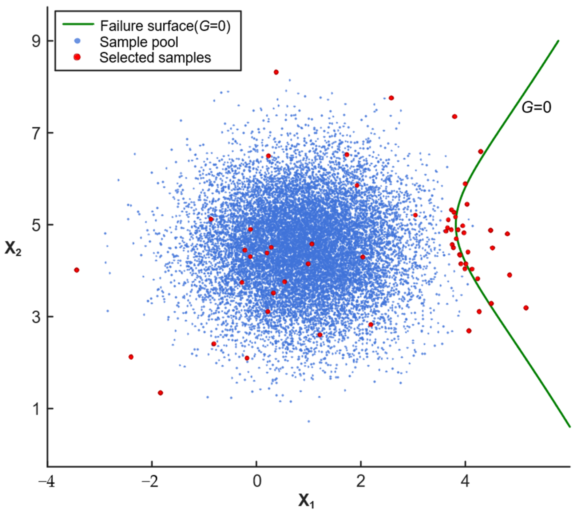
In this context, the probability of a sample point appearing in the stochastic design space defines its contribution (weight) to the analysis. In engineering practice, most sample points fall into the safe region, while those in the failure domain are extremely rare and carry very small weights. Therefore, increasing the sample density near the limit state surface can effectively enhance computational efficiency. To achieve this, and following the screening principle in Ref. [30], this study proposes a sample selection strategy specifically for the nested extremum-based BP method. This strategy considers the occurrence probability of each sample point as its weight. Samples with smaller weights are then specifically selected to build the training dataset for the neural network model.
Each sample point x i consists of c design variables, denoted by x i j ( j = 1 , 2 , , c ) . Assuming the design variables are mutually independent, the weight of the sample point is calculated as
η i = f 1 ( x i 1 ) f 2 ( x i 2 ) f c ( x i c )
For mutually dependent design variables, the sample point weight is calculated via the joint probability density function (JPDF), expressed as
η i = f 1 ( x i 1 ) f 2 ( x i 2 ) f c 1 , c ( x i c 1 , x i c )
where f c is the probability density function (PDF) of the c -th random variable, and f c 1 , c denotes the JPDF of the ( c 1 ) -th and c -th variables.
This screening filters out most safe-region points, retaining a dataset with a higher proportion of failure points. When combined with random samples from the design space, the built training set effectively covers different conditions across the entire design area.
Once the initial neural network is built, it is used to predict the responses for a new set of random sample points. The point with the smallest absolute output—which is the point closest to the limit state surface—is then selected.
Next, the extremum-based method is used to calculate the actual minimum of the time-dependent performance function for this specific point. The error between this actual value and the BP model’s prediction is then calculated. If the accuracy meets the target requirements, BPNN training is complete. Otherwise, this point and its actual minimum are added to the training set to retrain the model. This process repeats until the model accuracy near the limit state surface meets the requirements.
Figure 2 illustrates the schematic diagram of sample selection using the proposed method.

3.3. Nested Calculation Method for TRA

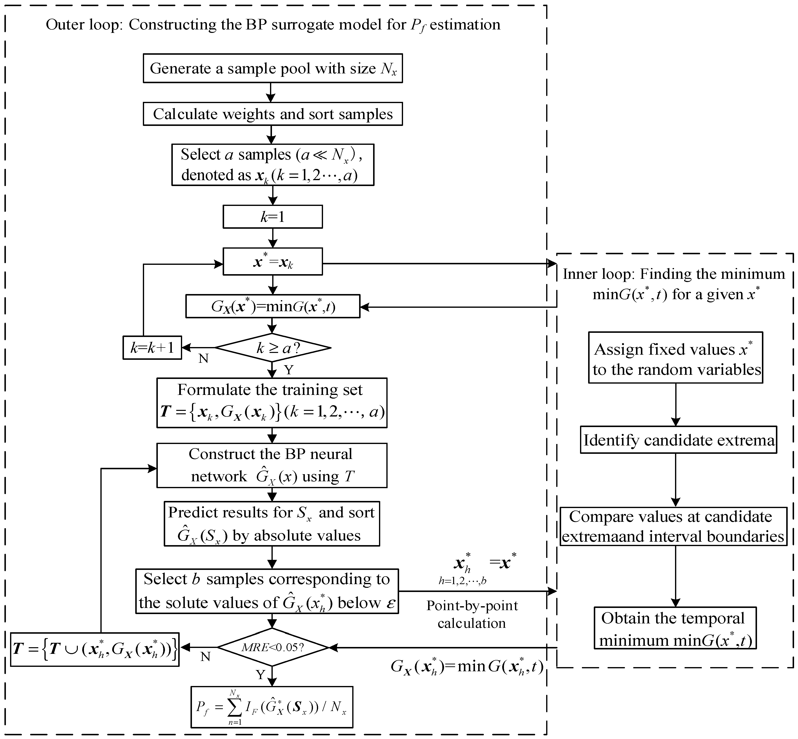
This paper proposes a nested method that combines the BPNN with the extremum-based method. The basic principle is that in the inner loop, the extremum-based method is used to find the minimum min G ( x * , t ) of the time-dependent performance function for a given realization x * of the uncertain variables. This transforms the time-dependent problem into an equivalent time-independent one. In the outer loop, the BPNN is used to handle high-dimensional and complex nonlinear problems. A BP model is established to map the input variables to the performance function minimum.
Finally, the trained BP model G ^ X * ( x ) is used to estimate the time-dependent failure probability. The detailed steps are as follows:
(1)
Generate the sample pool:
Generate a sample pool S x = x 1 , x 2 , , x N x of size N x using the joint PDF of the input variables X .
(2)
Calculate the weights of the sample points and sort them:
Pick the points with the lowest weights and randomly select additional points from the sample pool. Combine these into a training set of size a N x to ensure the dataset x k ( k = 1 , 2 , , a ) covers various conditions within the design space.
(3)
Calculate the minimum value:
Use various methods to calculate the minimum value min G ( x * , t ) of the time-dependent performance function when the uncertain variables are fixed at x * . Repeat a times to obtain the minimum of the performance function with respect to time for all sample points x k in the dataset, denoted by G X ( x k ) . These values are used to construct the training set T = x k , G X ( x k ) for the neural network.
(4)
Construct the BP neural network model:
Using the training set T , train the initial BPNN model. The sample point parameters x k serve as the inputs, and the minimum values G X ( x k ) serve as the outputs. The model is denoted by G ^ X ( x ) .
(5)
Validate the accuracy of the initial model:
Use model G ^ X ( x ) to predict the sample pool S x with a size of N x to obtain the output values G ^ X ( S x ) for all sample points. Select b points with absolute output values less than ε as verification points, denoted by G ^ X ( x h * ) . Use the extreme value method from Step 3 to calculate the minimum of the performance function with respect to time for the sample points G ^ X ( x h * ) corresponding to x h * ( h = 1 , 2 , , b ) (i.e., the points closest to the failure surface). This value is denoted by G X ( x h * ) . Finally, evaluate the error.
To measure model accuracy, metrics like Coefficient of Determination ( R 2 ) , Mean Absolute Error (MAE), and Mean Relative Error (MRE) are commonly used. In structural reliability, performance function values can vary significantly in scale depending on the specific problem. Accordingly, MRE is adopted as the error metric in this study, which is calculated as
M R E = 1 b h = 1 b G X ( x h * ) G ^ X ( x h * ) G X ( x h * )
where G ^ X ( x h * ) and G X ( x h * ) are the BP model output value and the actual minimum value of the performance function for the h-th sample point, respectively. b represents the number of samples used for error evaluation. A smaller value indicates higher model accuracy, but the required computational cost may increase. To balance computational efficiency and accuracy, the allowable MRE is set to be less than 0.05. In practical applications, the value of MRE can be appropriately reduced to improve the output accuracy of the model.
(6)
Model validation:
If the model accuracy meets the requirements, proceed to the next step. Otherwise, add the verification points x h * and their actual minima G X ( x h * ) to the training set T and retrain the model. Repeat the above steps until the accuracy satisfies the error requirements to obtain a qualified outer layer model G ^ X ( x ) .
(7)
Calculate failure probability:
Calculate the failure probability using the trained model. Input the sample pool S x into the trained BPNN model G ^ X ( x ) to obtain the predicted response and calculate the structural failure probability using Equation (16).
P f = n = 1 N x I F ( G ^ X ( S x ) ) / N x
The algorithm flowchart is shown in Figure 3.
Upon training completion, a convergence check is performed. The coefficient of variation ( C O V ) of the failure probability P f is calculated. This value measures the error between the estimated P f and its true value. A smaller C O V shows that the results are more reliable. The formula is as follows:
C O V P f = 1 P f P f N x
In this study, the condition C O V P f 0.05 serves as the verification criterion. If this condition is met, the calculated results are considered reliable. If C O V P f > 0.05 occurs, it means the sample size for calculating P f is insufficient. In this case, increase the sample size and recalculate the failure probability.

4. Case Study

4.1. Four-Bar Linkage Mechanism

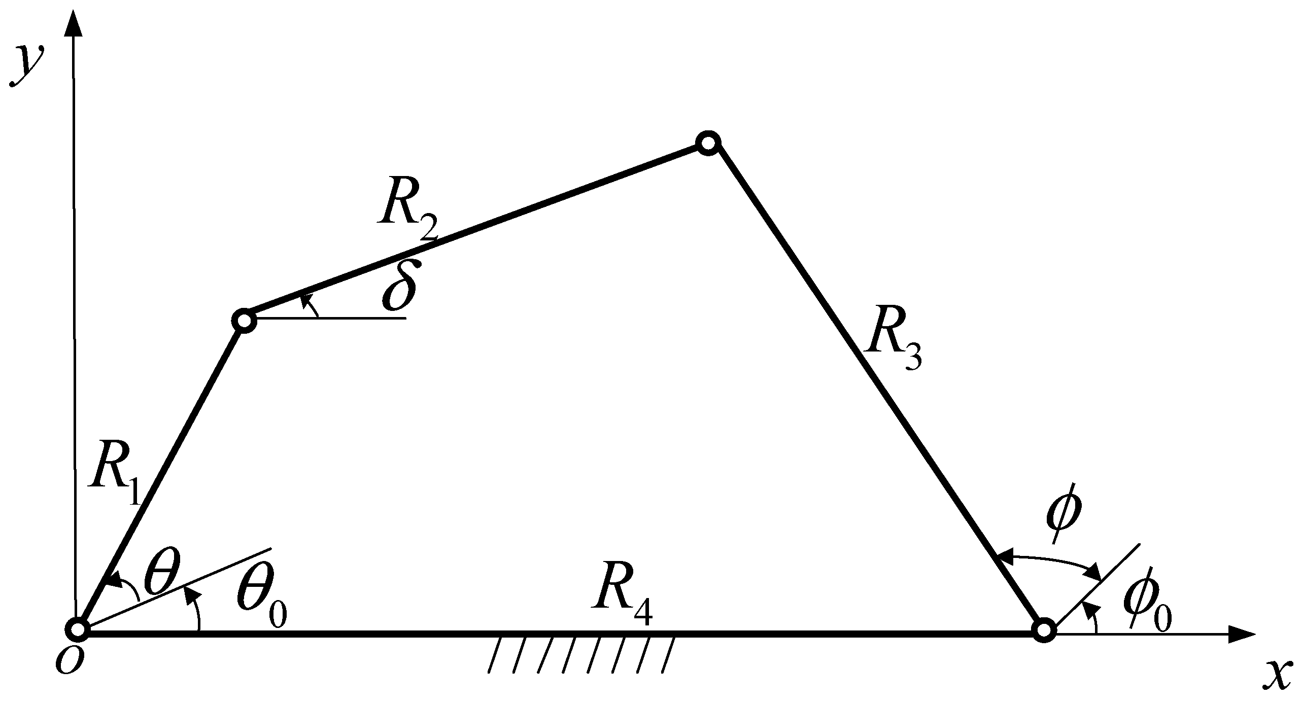
Figure 4 shows the four-bar linkage mechanism [31]. The geometric dimensions of the bars are defined by variables X = ( R 1 , R 2 , R 3 , R 4 ) and X i ( i = 1 , 2 , 3 , 4 ) . Their mean values are μ X 1 = 53 mm, μ X 2 = 122 mm, μ X 3 = 66.5 mm, and μ X 4 = 100 mm, respectively, and the standard deviations are σ X 1 = σ X 2 = σ X 3 = σ X 4 = 0.10 mm. All variables are assumed to follow normal distributions. The kinematic relationship of the four-bar linkage during motion is given by
R 1 cos θ + R 2 cos δ R 3 cos φ R 4 = 0 R 1 sin θ + R 2 sin δ R 3 sin φ = 0
where θ is regarded as the input of the motion process, while ϕ and δ are regarded as the outputs.
Based on Equation (18), the expressions for ϕ and δ can be obtained as
ϕ = 2 arc tan D ± D 2 + E 2 F 2 E + F δ = arc tan R 3 sin φ R 1 sin θ R 4 + R 3 cos φ R 1 cos θ
where
D = 2 R 1 R 3 sin θ
E = 2 R 3 ( R 4 R 1 cos θ )
F = R 2 2 R 1 2 R 3 2 R 4 2 + 2 R 1 R 4 cos θ
This case focuses on the output angle ϕ . The time-dependent output function is
ϕ d = 76 ° + 60 ° sin ( 3 ( θ 95.5 ° ) / 4 )
The reliability of this mechanism depends on whether the output error exceeds a threshold c . The mechanism is reliable if the error stays below this limit; otherwise, it fails. Considering the angle θ as the time variable t , the performance function is defined as
G ( R 1 , R 2 , R 3 , R 4 , t ) = c abs ϕ ϕ d
The domain of t is set to [ 95.5 ° , 155.5 ° ] . The error threshold c is a deterministic value of 0.8.
Calculations were performed using three approaches: the MCS, the Kriging method, and the proposed method in this study. A comparison of the results is presented in Table 1. In this example, the extremum-based method is used in the inner loop. Because this method accurately finds the time-dependent performance function minimum, the outer-layer model produces highly accurate results. According to Table 1, the MCS generated 2 18 sample points, and the time domain was uniformly discretized into 101 time points. This required calling the performance function ( N c a l l ) a total of 2 18 × 101 times, resulting in a failure probability ( P f ) of 2.30 × 10 3 . For the Kriging-based method, the calculated failure probability was 2.38 × 10 3 , with a total of 1236 calls to the performance function, and the proposed method only requires 692 times to obtain a failure probability of 2.32 × 10 3 . These results show that the proposed method is both accurate and efficient.

4.2. Aero-Engine Turbine Disc

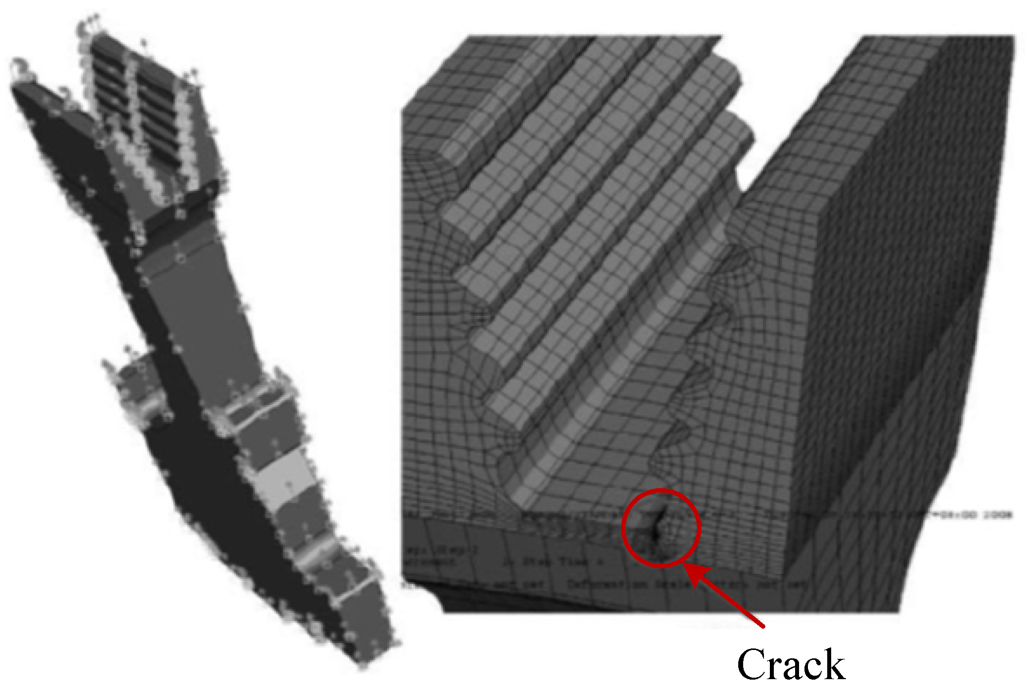
Case 2 considers an aero-engine turbine disc, as shown in Figure 5 [32]. Under operating conditions, the disc is subjected to large centrifugal forces. Stress concentration occurs at the bottom of the dovetail slot. The structure fails if the external load exceeds the load-bearing capacity, causing cracks at these locations.
During operation, the loads acting on the turbine disc are
φ ( C , ρ , J , θ , n 0 ) = C ω 2 2 π + 2 ρ ω 2 J
The cross-sectional area and ultimate strength of the disc are A and σ s , respectively. The load-bearing capacity is then F = σ s A . Accordingly, the performance function of the disc is given by
G ( σ s , ρ , C , A , J , θ , n 0 ) = F ( σ s , A ) φ ( C , ρ , J , θ , n 0 )
where C , ρ , and J denote the rotation coefficient, density, and section moment of inertia of the turbine disc, respectively. The rotational angular velocity ω is related to the rotational frequency n , which is determined by ω = 2 n π , n = n 0 sin ( 0.1 ( θ / 3 ) + 0.65 ) , and θ [ 0 , 2 π ] . The angle θ is regarded as the time parameter. Structural failure is defined to occur when G 0 .
The statistical parameters of the six mutually independent random variables C , ρ , J , n 0 , σ s and A are summarized in Table 2. All variables follow normal distributions.
In case 2, the failure criterion is defined as the load exceeding the ultimate strength. Compared with Case 1, the performance function in this case exhibits a wider range of variation. Calculations are conducted using different methods. Table 3 lists the results.
According to Table 3, the MCS uses 2 × 10 7 function calls, and the failure probability is 3.99 × 10 3 . For the Kriging method, 505 calls to the performance function are needed, with a relative error of 1.75%, and the proposed method requires 485 calls to obtain a failure probability of 4.05 × 10 3 . The relative error is 1.75%, indicating that the results obtained by the three methods are in close agreement.
These results demonstrate that the proposed method remains favourable computational performance even for problems with large variations, proving its suitability for practical engineering applications.

4.3. Cantilever Tube

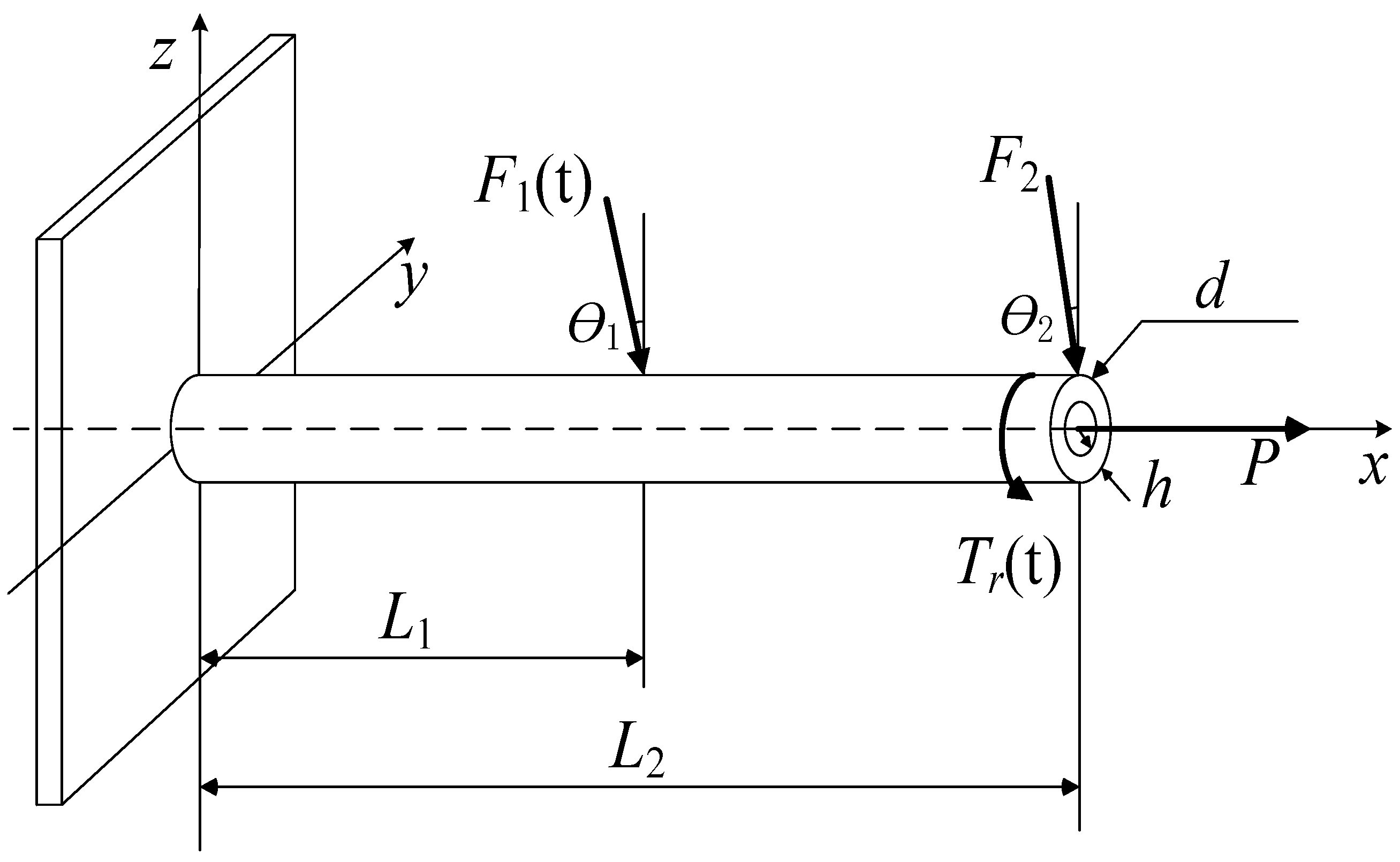
Case 3 considers a cantilever tube model [33], as shown in Figure 6. The material yield strength is R 0 . The structure is subjected to three external loads ( F 1 ( t ) , F 2 , P ) and a torque T r ( t ) . A failure occurs if the maximum stress exceeds the material yield strength. F 1 ( t ) and T r ( t ) are Gaussian random processes, with the autocorrelation functions expressed as
ρ F 1 t 1 , t 2 = exp t 2 t 1 / 4
ρ T r t 1 , t 2 = exp t 2 t 1 2 / 0.5 2
Analysis shows that the maximum stress of the cantilever tube structure is a function of its diameter d , thickness h , three external loads ( F 1 ( t ) , F 2 , P ), and torque T r ( t ) . The material strength R decreases over time according to R ( t ) = R 0 ( 1 0.01 t ) .
The material strength R degrades over time, denoted by R ( t ) = R 0 ( 1 0.01 t ) . Accordingly, the performance function of this model is defined as the difference between the strength R and the maximum stress, which is
G ( X , t ) = R ( t ) σ x 2 ( t ) + 3 τ z x 2 ( t )
where
σ x ( t ) = F 1 ( t ) sin ( θ 1 ) + F 2 sin ( θ 2 ) + P A + M ( t ) d 2 I
τ z x ( t ) = T r ( t ) d 4 I
M ( t ) = F 1 ( t ) cos ( θ 1 ) L 1 + F 2 sin ( θ 2 ) L 2
and
A = π 4 d 2 ( d 2 h ) 2
I = π 64 d 4 ( d 2 h ) 4
The time interval of interest is [ 0 , 5 ] years, uniformly discretized into 100 samples. The statistical parameters of the five mutually independent random variables d , h , R 0 , F 2 and P are summarized in Table 4. All variables follow normal distributions.
Additional parameters include L 1 = 60   mm , L 2 = 120   mm , θ 1 = 10 ° and θ 2 = 5 ° . The stochastic processes F 1 ( t ) and T r ( t ) are represented by 25 and 13 independent standard normal variables, respectively, using the KL expansion. These expansions retain 99.03 % and 99.2 % of the variance, resulting in a total of 43 random input variables.
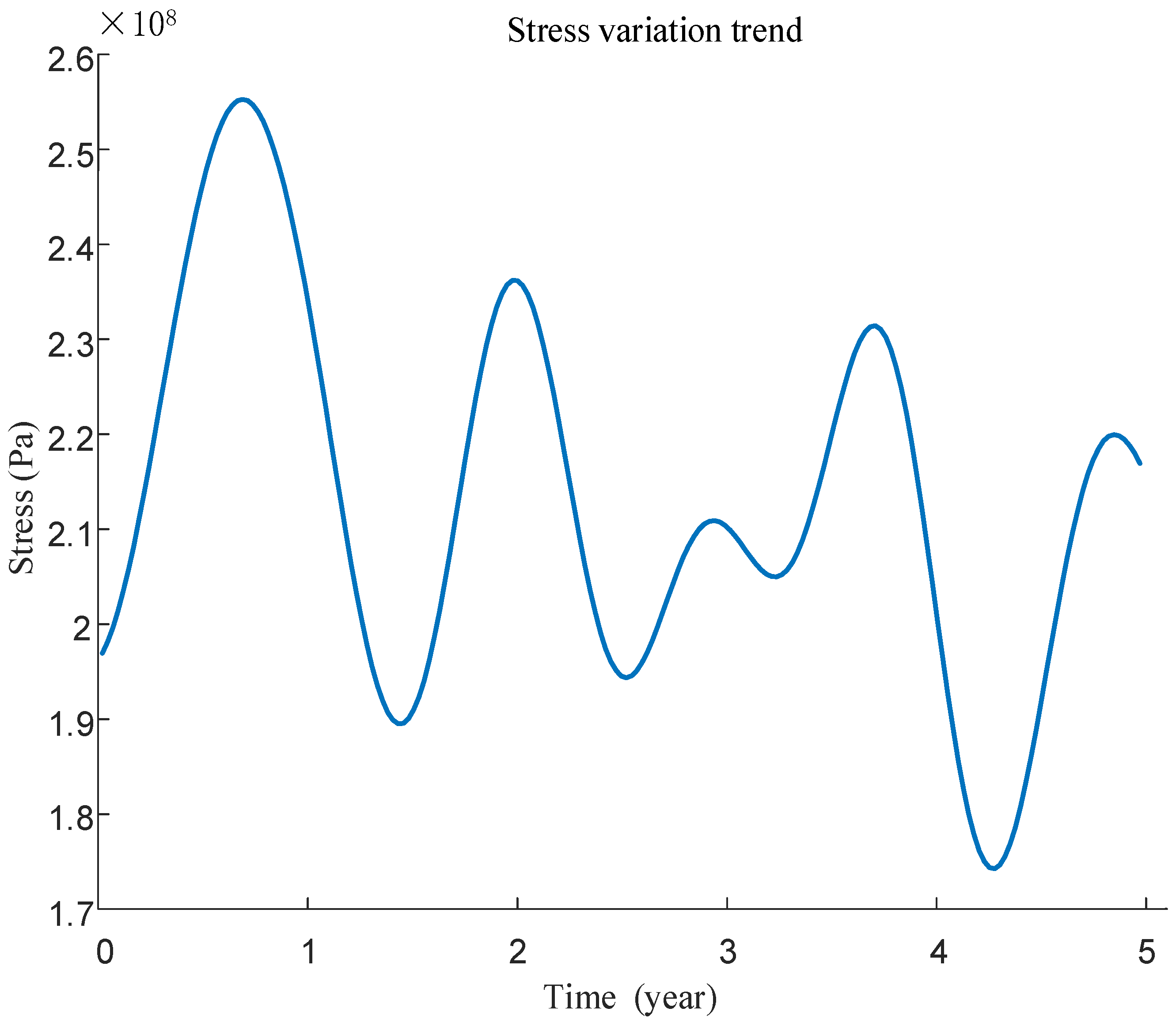
Figure 7 shows the stress variation in the cantilever tube over time for mean values of the input variables d , h , R 0 , F 2 and P . The performance function in this case exhibits strong nonlinearity.
To handle the stochastic processes, an interpolation method is employed. Through KL expansion, these processes are represented by 43 random variables. For each realization, 25 time points are uniformly selected to evaluate the performance function. An interpolation function is then constructed to identify the minimum over the time interval. This extremum is applied to train the surrogate model. Table 5 summarizes the results.
Compared with traditional surrogate models, the BPNN handles high-dimensional and nonlinear problems more effectively. According to Table 5, the proposed method requires 3375 function evaluations, and the Kriging method used 8400 calls to the performance function to complete the calculation. These results demonstrate that the proposed method is suitable for engineering problems involving high dimensionality and nonlinearity.

5. Conclusions

TDSSs in aerospace engineering often involve high dimensionality, nonlinearity, and complex uncertainty. However, neural networks show significant advantages in addressing such challenges. Based on this characteristic, this paper proposes a reliability analysis method combining the BPNN with the extremum-based method.
The proposed method adopts a double-loop structure. Specifically, the inner loop finds the minimum of the time-dependent performance function for a given realization of the random inputs, thereby transforming the time-dependent problem into a time-independent one. Then, the outer loop constructs the BPNN to map the relationship between the random variables and these minima. To improve convergence efficiency, an adaptive sample selection strategy is integrated into the training process. Once the stopping criterion is satisfied, the failure probability of the TDSS is estimated using the MCS.
Section 4 gives the specific procedures of the proposed method. Then, the method is applied to a four-bar linkage, an aero-engine turbine disc, and a cantilever tube, which cover low-dimensional conventional time-dependent problems, problems with large fluctuations in performance function values, and high-dimensional strongly nonlinear problems. The results verify the rationality and applicability of the proposed method for engineering purposes. Compared with the MCS, the proposed method remains accurate, with small relative errors between the results. In contrast to the nested calculation method of the same type using the Kriging model, the proposed method improves computational efficiency, particularly demonstrating significant advantages in handling high-dimensional and nonlinear problems. This is attributed to the BPNN’s powerful fitting ability for complex nonlinear problems.
Furthermore, the method proposed in this paper possesses excellent engineering extensibility with multiple practical application advantages: the neural network model used in the outer layer retains effective sample point information near the failure surface during training, making it suitable for reliability-based design optimization (RBDO) in practical engineering. The proposed method can be integrated with the hybrid uncertainty handling method, expanding its adaptability to scenarios with multiple coexisting uncertainties such as randomness and fuzziness. Additionally, some classical algorithms can be flexibly incorporated for the neural network architecture to achieve its optimization and enhance computational efficiency and accuracy.

Author Contributions

Conceptualization, G.L. and G.X.; methodology, G.L.; software, G.L.; validation, G.L., Y.H. and L.Z.; formal analysis, G.L.; investigation, G.L.; resources, G.L.; data curation, G.L.; writing—original draft preparation, G.L.; writing—review and editing, G.L. and G.X.; visualization, G.L.; supervision, G.X.; project administration, G.X.; funding acquisition, G.X. All authors have read and agreed to the published version of the manuscript.

Funding

This research was funded by Science Challenge Project (No. TZ2025003) and the National Natural Science Foundation of China (Grant No. NSFC 52275143).

Data Availability Statement

Data is contained within the article.

Acknowledgments

The authors would like to express their sincere gratitude to the National Key Laboratory of Strength and Structural Integrity for providing research facilities and support. Their contribution was essential for the multi-source uncertainty modelling and reliability analysis presented in this study. Finally, we appreciate the editors and reviewers of Aerospace for their insightful comments and efforts in improving the quality of this paper.

Conflicts of Interest

The authors declare no conflicts of interest.

Abbreviations

The following abbreviations are used in this manuscript:
BPNNBack Propagation Neural Network
MCSMonte Carlo Simulation
ISImportance Sampling
RSMResponse Surface Methods
WWeight
BBias
MSEMean Squared Error
COVCoefficient of Variation
TDSSTime-dependent Structural Systems
RBDOReliability-Based Design Optimization
FEMFinite Element Model
TRATime-dependent Reliability Analysis
PDFProbability Density Function
JPDFJoint Probability Density Function
ReLURectified Linear Unit
RBFRadial basis function
ACOAnt Colony Optimization
GAGenetic algorithms
SASimulated annealing
MREMean Relative Error
MAEMean Absolute Error
EOLEExpansion Optimal Linear Estimation
KLKarhunen–Loéve
R 2 Coefficient of Determination

References

  1. Der Kiureghian, A. Structural and System Reliability; Cambridge University Press: Cambridge, UK, 2022. [Google Scholar]
  2. Wang, C.; Beer, M.; Ayyub, B.M. Time-dependent reliability of aging structures: Overview of assessment methods. ASCE-ASME J. Risk Uncertain. Eng. Syst. Part A Civ. Eng. 2021, 7, 03121003. [Google Scholar]
  3. Yuan, X.; Liu, S.; Faes, M.; Valdebenito, M.; Beer, M. An efficient importance sampling approach for reliability analysis of time-variant structures subject to time-dependent stochastic load. Mech. Syst. Signal Process. 2021, 159, 107699. [Google Scholar]
  4. Rice, S.O. Mathematical analysis of random noise. Bell Syst. Technol. J. 1945, 24, 146–156. [Google Scholar]
  5. Andrieu-Renaud, C.; Sudret, B.; Lemaire, M. The PHI2 method: A way to compute time-variant reliability. Reliab. Eng. Syst. Saf. 2004, 84, 75–86. [Google Scholar] [CrossRef] [Scilit]
  6. Zhang, Y.; Xu, J.; Gardoni, P. A loading contribution degree analysis-based strategy for time-variant reliability analysis of structures under multiple loading stochastic processes. Reliab. Eng. Syst. Saf. 2024, 243, 109833. [Google Scholar]
  7. Meng, Z.; Zhao, J.; Jiang, C. An efficient semi-analytical extreme value method for time-variant reliability analysis. Struct. Multidiscip. Optim. 2021, 64, 1469–1480. [Google Scholar]
  8. Zio, E. The Monte Carlo Simulation Method for System Reliability and Risk Analysis; Springer: London, UK, 2013. [Google Scholar]
  9. Wang, J.; Cao, R.; Sun, Z. Importance sampling for time-variant reliability analysis. IEEE Access 2021, 9, 20933–20941. [Google Scholar] [CrossRef] [Scilit]
  10. Guo, H.; Dong, Y.; Gardoni, P. Adaptive subset simulation for time-dependent small failure probability incorporating first failure time and single-loop surrogate model. Struct. Saf. 2023, 102, 102327. [Google Scholar]
  11. Yang, X.; Jiang, W.; Zhang, Y.; Zhao, J. An active learning method combining MRBF model and dimension-reduction importance sampling for reliability analysis with high dimensionality and very small failure probability. Reliab. Eng. Syst. Saf. 2025, 261, 111107. [Google Scholar] [CrossRef] [Scilit]
  12. Yang, X.; Chen, P.; Chen, L.; Wei, Y.; Jiang, W. Active learning for high-dimensional reliability using matrix-operation anisotropic RBF model embedded with Multiscale Graph Correlation. Comput. Methods Appl. Mech. Eng. 2025, 446, 118286. [Google Scholar]
  13. Yang, X.; Zhang, Y.; Chen, P.; Yang, F. An active learning method for high-dimensional and small failure probability problems combining matrix-operation radial basis function model with matrix-operation hybrid optimization algorithm. Comput. Struct. 2025, 319, 108007. [Google Scholar] [CrossRef] [Scilit]
  14. Choi, Y.; Ahn, J.; Chang, D. Time-dependent reliability analysis of plate-stiffened prismatic pressure vessel with corrosion. Mathematics 2021, 9, 1544. [Google Scholar] [CrossRef] [Scilit]
  15. Feng, K.; Wang, L.; Shi, Y. Time-Dependent Reliability Analysis Method Under Evidence Uncertainty. AIAA J. 2025, 1–11. [Google Scholar] [CrossRef] [Scilit]
  16. Afshari, S.S.; Zhao, C.; Zhuang, X.; Liang, X. Deep learning-based methods in structural reliability analysis: A review. Meas. Sci. Technol. 2023, 34, 072001. [Google Scholar] [CrossRef] [Scilit]
  17. Zhang, D.; Han, X.; Jiang, C.; Liu, J.; Li, Q. Time-dependent reliability analysis through response surface method. J. Mech. Des. 2017, 139, 041404. [Google Scholar] [CrossRef] [Scilit]
  18. Shi, Y.; Lu, Z.; He, R. Advanced time-dependent reliability analysis based on adaptive sampling region with Kriging model. Proc. Inst. Mech. Eng. Part O J. Risk Reliab. 2020, 234, 588–600. [Google Scholar] [CrossRef] [Scilit]
  19. Zafar, T.; Zhang, Y.; Wang, Z. An efficient Kriging based method for time-dependent reliability based robust design optimization via evolutionary algorithm. Comput. Methods Appl. Mech. Eng. 2020, 372, 113386. [Google Scholar] [CrossRef] [Scilit]
  20. Xu, Z.; Wang, H.; Zhao, K.; Zhang, H. Structural reliability analysis using gradient-enhanced physics-informed neural network and probability density evolution method. Struct. Saf. 2025, 116, 102604. [Google Scholar] [CrossRef] [Scilit]
  21. Guo, H.; Zhang, J.; Dong, Y.; Frangopol, D.M. Probability-informed neural network-driven point-evolution kernel density estimation for time-dependent reliability analysis. Reliab. Eng. Syst. Saf. 2024, 249, 110234. [Google Scholar] [CrossRef] [Scilit]
  22. Wang, Z.; Wang, P. A nested extreme response surface approach for time-dependent reliability-based design optimization. J. Mech. Des. 2012, 134, 121007. [Google Scholar] [CrossRef] [Scilit]
  23. Li, H.; Lu, Z.; Feng, K. A double-loop Kriging model algorithm combined with importance sampling for time-dependent reliability analysis. Eng. Comput. 2024, 40, 1539–1558. [Google Scholar] [CrossRef] [Scilit]
  24. Shi, Y.; Beer, M. Physics-informed neural network classification framework for reliability analysis. Expert Syst. Appl. 2024, 258, 125207. [Google Scholar] [CrossRef] [Scilit]
  25. Vicario, G.; Craparotta, G.; Pistone, G. Meta-models in computer experiments: Kriging versus artificial neural networks. Qual. Reliab. Eng. Int. 2016, 32, 2055–2065. [Google Scholar] [CrossRef] [Scilit]
  26. Zhang, D.; Li, Y.; Fu, Z.; Wang, Y.; Xu, K. Fatigue reliability analysis of bogie frames considering parameter uncertainty. Int. J. Fatigue 2025, 190, 108632. [Google Scholar] [CrossRef] [Scilit]
  27. Cheridito, P.; Jentzen, A.; Rossmannek, F. Efficient approximation of high-dimensional functions with neural networks. IEEE Trans. Neural Netw. Learn. Syst. 2021, 33, 3079–3093. [Google Scholar] [CrossRef] [Scilit]
  28. Zhao, Y.; Zhang, D.; Yang, M.; Wang, F.; Han, X. On efficient time-dependent reliability analysis method through most probable point-oriented Kriging model combined with importance sampling. Struct. Multidiscip. Optim. 2024, 67, 6. [Google Scholar] [CrossRef] [Scilit]
  29. Şenol, H.; Çırpan, H.A.; Panayırcı, E. Linear expansions for frequency selective channels in OFDM. AEU-Int. J. Electron. Commun. 2006, 60, 224–234. [Google Scholar] [CrossRef] [Scilit]
  30. Song, X.; Zou, L.; Tang, M. An improved Monte Carlo reliability analysis method based on BP neural network. Appl. Sci. 2025, 15, 4438. [Google Scholar] [CrossRef] [Scilit]
  31. Zhang, J. An Improved Envelope Method for Time-Dependent Mechanism Reliability. J. Mech. Des. 2025, 147, 051706. [Google Scholar] [CrossRef] [Scilit]
  32. Ling, C.; Lu, Z.; Feng, K.; Sun, B. Efficient numerical simulation methods for estimating fuzzy failure probability based importance measure indices. Struct. Multidiscip. Optim. 2019, 59, 577–593. [Google Scholar] [CrossRef] [Scilit]
  33. Liu, Y.; Li, L.; Zhao, S.; Zhou, C. A reliability analysis method based on adaptive Kriging and partial least squares. Probabilistic Eng. Mech. 2022, 70, 103342. [Google Scholar] [CrossRef] [Scilit]
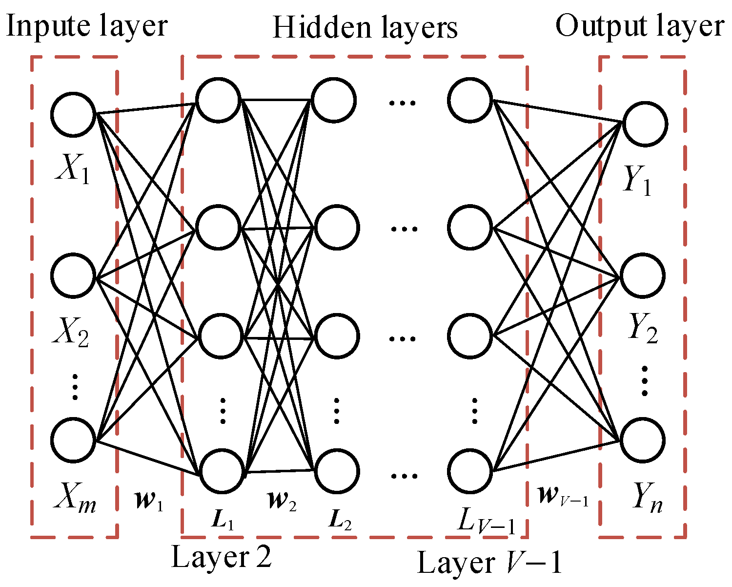
Figure 1. Schematic diagram of the BPNN structure.
Aerospace 13 00146 g001
Figure 2. Schematic diagram of sample selection.
Aerospace 13 00146 g002
Figure 3. Computational flowchart.
Aerospace 13 00146 g003
Figure 4. Schematic diagram of the four-bar linkage mechanism.
Aerospace 13 00146 g004
Figure 5. Aero-engine turbine disc.
Aerospace 13 00146 g005
Figure 6. Schematic diagram of the cantilever tube model.
Aerospace 13 00146 g006
Figure 7. Stress–time variation diagram.
Aerospace 13 00146 g007
Table 1. Computing results of case 1.
Method P f C O V P f N c a l l Error
MCS 2.30 × 10 3 4.07 × 10 2 2 18 × 101 = 26 , 476 , 544 /
Kriging 2.38 × 10 3 4.00 × 10 2 12363.36%
Proposed 2.32 × 10 3 4.05 × 10 2 6920.86%
Table 2. Distribution parameters of random variables in turbine disc structure.
VariablesDistribution TypeMean ValueStandard Deviation
σ s / N m 2 Normal 1.10 × 10 9 1.10 × 10 8
A / m 2 Normal 6.20 × 10 3 6.20 × 10 4
C Normal5.76 5.76 × 10 1
ρ / kg m 3 Normal8240824
J / m 4 Normal 1.22 × 10 4 1.22 × 10 5
n 0 Normal22022
Table 3. Computing results of case 2.
Method P f C O V P f N c a l l Error
MCS 3.99 × 10 3 3.53 × 10 2 2 × 10 5 × 100 = 2 × 10 7 /
Kriging 3.92 × 10 3 3.56 × 10 2 505 1.75 %
Proposed 4.05 × 10 3 3.51 × 10 2 485 1.50 %
Table 4. Distribution parameters of random variables in cantilever tube model.
VariablesDistribution TypeMean ValueStandard Deviation
d / mm Normal420.42
h / mm Normal50.10
R 0 / Mpa Normal56056
F 2 / N Normal1900190
P / N Normal1000100
F 1 ( t ) / N Gaussian Process1900190
T r ( t ) / N Gaussian Process1800180
Table 5. Computing results of case 3.
Method P f C O V P f N c a l l Error
MCS 3.30 × 10 3 4.82 × 10 2 100 × 10 5 = 10 7 /
Kriging 3.25 × 10 3 4.86 × 10 2 8400 1.52 %
Proposed 3.24 × 10 3 4.86 × 10 2 3375 1.82 %
Disclaimer/Publisher’s Note: The statements, opinions and data contained in all publications are solely those of the individual author(s) and contributor(s) and not of MDPI and/or the editor(s). MDPI and/or the editor(s) disclaim responsibility for any injury to people or property resulting from any ideas, methods, instructions or products referred to in the content.