Increasing Downlink Efficiency for Fly-By Imaging Missions Through Convolutional Neural Network-Based Data Reduction

Abstract

Data transmission requirements are a major constraint for mission design and can increase mission complexity significantly. Thus, reducing the amount of data required to be transmitted is key. In this work, the reference scenario of the European Space Agency’s Comet Interceptor mission, specifically its Optical Periscopic Imager for Comets (OPIC) instrument, is used to assess the possibilities for onboard data selection through convolutional neural networks. In this study, we train various semantic segmentation and object detection networks to automatically determine the most scientifically interesting area on a fly-by image of a comet, focusing on the nucleus and inner coma, and investigate the impact this could have on data reduction. In the context of computational complexity, the average dice coefficient dropped by 0.07 between the best performing and the smallest network for semantic segmentation and by 0.11 for detection networks. While this drop is significant, the more computationally complex networks did not lead to any significant accuracy improvement. Based on the results, we can conclude that using convolutional neural networks is a feasible strategy for reducing data budgets in comet fly-by missions and that even the simplest segmentation networks tested can achieve a meaningful performance, showing that this approach is even feasible on hardware that can be compatible for launch or has already been used in space.

1. Introduction

The increasing volume and complexity of data generated by modern imaging instruments have made data transmission a primary constraint in both terrestrial and space-based applications [1,2]. In space missions in particular, limited downlink bandwidth, intermittent communication windows, and strict power budgets significantly restrict the amount of raw data that can be transmitted to ground stations. As a result, intelligent onboard data reduction and selection strategies are becoming a key enabling technology for future missions. This spans from traditional Machine Learning (ML) algorithms on missions like ExoMars [3] or more broadly as in [4] to cosmology missions using Convolutional Neural Networks (CNN) as in [5] and, last but not least, to diverse Earth observation applications using diverse ML methods as surveyed in [6] and boundary pushing onboard learning concepts as in [7].

This alone shows that onboard data reduction can be achieved in multiple ways, including data compression and data prioritisation. While compression can be used for data reduction, it can introduce issues with noise that is typically present in real imagery. Another option is to use automated systems to determine the most useful information in the raw data flow and downlink only the highest-priority fraction. In the case of scientific images, this would involve selecting images that contain the mission target and cropping the relevant regions. Recent advances in CNNs have demonstrated strong capabilities in extracting semantically relevant information from high-dimensional data [8], motivating their use for autonomous data handling under constrained conditions [9], and in this article, we investigate this avenue.

1.1. Terrestrial Applications of CNN-Based Data Reduction

In terrestrial applications, CNN-based data reduction and selection techniques are widely adopted in domains such as autonomous driving, medical imaging, remote sensing [10], and industrial inspection [11]. In these contexts, semantic communication [12], semantic segmentation [13], and object detection networks are commonly used to identify regions of interest while discarding background information. This enables significant reductions in data storage, transmission, and processing requirements without compromising task-relevant information. High computational resources, continuous connectivity, and the availability of large annotated datasets have accelerated the development and deployment of such approaches on Earth, establishing CNNs as a mature and reliable technology for perception-driven data filtering.

1.2. Space-Specific Challenges in CNN-Based Data Reduction

Despite their success in terrestrial environments, the direct transfer of CNN-based methods to space applications remains challenging. Processing systems onboard spacecraft are subject to severe constraints on computational power, memory, energy consumption, and radiation tolerance. Additionally, space missions often operate in environments that differ significantly from those represented in typical training datasets, limiting the transferability of networks trained on terrestrial ground truth data. The need for high reliability, deterministic behaviour, and long-term autonomy further complicates the deployment of complex neural networks onboard spacecraft. These challenges necessitate careful evaluation of network architectures, model sizes, and performance trade-offs when considering CNN-based onboard processing for space missions.

1.3. Related Work in Space Applications

Recent years have seen an increasing interest in the application of machine learning techniques for onboard data processing in space, as mentioned in the previously introduced references [5,6,7,9]. This interest has not only persisted but also led to various deployments [14,15]. Industrial and research initiatives such as by KappaZetta [16] and KP Labs [17] have demonstrated the feasibility of deploying CNNs on space-qualified hardware for tasks including image classification, segmentation, and event detection. Several missions and technology demonstrators have explored autonomous image selection and compression using neural networks to reduce downlink requirements.

One of the best documented examples in this field is Φsat-1, which used CloudScout CNN [9] onboard for detecting clouds and linking down only the least cloudy images [15]. They achieved 90% reduction [18] in data downlink volume. Also, Φsat-1 used Fully Connected Network(FCN)-based segmentation map for flood mapping [19] instead of downlinking multi-band images, resulting in a 100-fold reduction in data budget. Φsat-1 used Intel Movidus 2 [20] as its Artificial Intelligence (AI) acceleration platform.

CogniSAT-6 also demonstrated cloud removal and compression [21,22] by dividing the image into tiles and downlinking and compressing only tiles that were considered cloud-free. Total compression ratio was reported to be 1.99 to 2.30, meaning roughly 50–60% data reduction. They used their custom CogniSAT-XE2 AI coprocessing board, based on Myriad X.

Another set of data reduction experiments was conducted on HYPSO-1, with detailed publications providing an in-depth look. It was initially introduced in [23] with the first results presented in [24], and the network and deployment strategy detailed in [25]. They used 1D-Justo-LiuNet, a one-dimensional CNN on Zynq-7030 System-on-Chip with a Kintex-7 Field Programmable Gate Array (FPGA). While the tests were considered successful, no information that could be treated as a data reduction metric has been found.

Data reduction has also been tested for space debris detection [26], where over 93% data reduction was claimed by considering only streaks detected from images. This research used the You Only Look Once (YOLO) model named v4-tiny [27]. These studies indicate that meaningful data reduction can be achieved onboard, but also highlight the importance of task-specific network design, robust training data, and realistic evaluation under mission-relevant conditions.

1.4. Hypothesis of Transfer to Space Applications

Building on these developments, this work hypothesises that CNN-based semantic segmentation and object detection networks can be effectively used for onboard data reduction in cometary imaging scenarios. By identifying and selectively transmitting only semantically relevant pixels or regions, a substantial reduction in downlink data volume can be achieved compared to conventional methods. Furthermore, it is hypothesised that networks trained on synthetically generated datasets can generalise sufficiently well to enable reliable performance under realistic mission constraints. This hypothesis reflects a sim-to-real training paradigm, in which models trained primarily on synthetic data are expected to transfer effectively to real mission observations. This study evaluates these hypotheses using the application scenario of the European Space Agency (ESA) Comet Interceptor [28,29] mission, which targets a dynamically new comet that would be selected after the mission has already launched [30], with particular focus on achievable data reduction, detection reliability, and deployability on resource-constrained onboard systems. Specifically, we are viewing the situation from Optical Periscopic Imager for Comets (OPIC) viewpoint [31]. Additionally, the results are compared with currently used algorithmic solutions in terms of algorithmic accuracy and data reduction.

• Can neural networks reliably detect cometary objects such as nuclei and dust jets?
• Can synthetically generated data enable high-precision data reduction through neural networks and reduce data more effectively than current state-of-the-art algorithms?
• How reliable are such detection methods in scenarios not considered in the synthetic dataset, and how is the behaviour in border cases?
• What theoretical computational cost is to be associated with these different factors?

How these questions are answered is outlined through the materials and methods, Section 2. Starting with the workflow, Section 2.1, materials used, Section 2.2 and Section 2.3, including applied augmentation, Section 2.4, networks used, in Section 2.6 and Section 2.7, as well as other algorithms in Section 2.5. Lastly, the training process is outlined in Section 2.8 and the following evaluation methods are introduced in Section 2.9.

The results, Section 3, are obtained by implementing the outlined methodology and are included in this section as raw data answering the questions in four parts. Section 3.1 describes the qualitative (visual) analysis performed on the dataset, Section 3.2 shows the dice metrics as a measure of accuracy, while Section 3.3 shows the precision as a measure of reliability, and Section 3.4 provides the results for raw data reduction. While Section 3.5 focuses on the accuracy compared to network complexity, Section 3.6 focuses on data reduction compared to network complexity.

Ultimately, the data are discussed in Section 4 in four parts. Firstly, data reduction in Section 4.1, then network complexity in Section 4.3, and lastly hardware deployability in Section 4.4. This follows future directions outlook, including potential training improvements Section 5.1, potential network optimisations to reduce complexity Section 5.2 and deployability Section 5.3. The paper is concluded with Section 6.

2. Materials and Methods

2.1. Workflow

This paper focuses on the development of application-specific CNNs aimed at maximising data reduction for the defined application scenario. This section aims to provide insight into the overall workflow. Firstly, the synthetically generated CometSet_v1-1 dataset, introduced in Section 2.2, was created to provide data for future comet fly-by or landing missions. Various augmentations are introduced as they are implemented. In the scope of this work, we focus on optimising data reduction using models trained on this dataset. This is explored through two network types: semantic segmentation and object detection. An extensive list of networks evaluated is provided in Section 2.6 and Section 2.7. As well-trained networks are the basis to perform the ultimate task of data reduction, significant effort was laid into creating a stable and adaptable training workflow, which is introduced in Section 2.8. This serves as the basis for the key part of the work. The evaluation in Section 2.9 provides an assessment of the different data reduction methods and their deployability in the real world based on existing data. The goal is to assess data reduction based on the synthetic masks, allowing us to make an absolute statement about how many pixels were of interest in this image. The evaluation therefore considers not only how many relevant pixels can be detected and transmitted, but also how the CNNs compare with currently deployed methods.

2.2. Comet Dataset

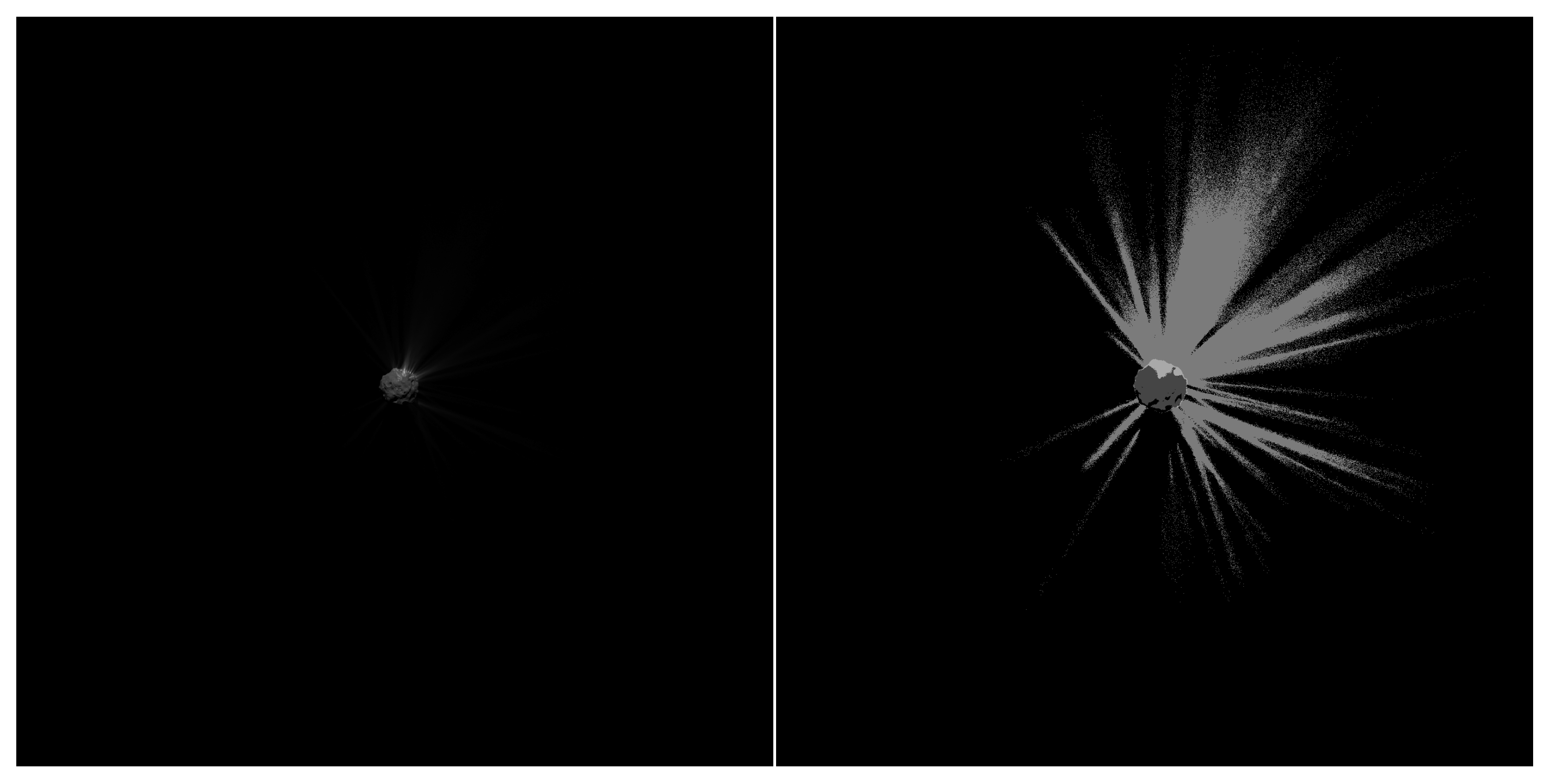
CometSet is a custom-generated dataset of cometary bodies focusing on the realistic simulation of comet shapes and dust jets. This was achieved with the Fly-By Generation (FlyByGen) tool [32], which is based on Blender and its Cycles rendering engine [33]. FlyByGen and the dataset were created to support the simulation of fly-by scenarios relevant to the ESA Comet Interceptor mission. FlyByGen is also used to validate and verify the image-capture scenarios and control gateware for the OPIC instrument on the Comet Interceptor mission. The dataset contains 2000 randomly generated comet nucleus-like objects, each rendered from 14 different perspectives. For the base dataset, the object (nucleus with its surrounding coma) is always in the centre of the Field of View (FoV). Each image is first rendered with all elements (nucleus, jets, dust) included and then for each element separately to obtain separate nucleus and dust renders. These separate renders allow the creation of synthetic masks, which are used as ground truth for this study. Examples can be seen in Figure 1. The dataset is available on Zenodo as CometSet v1.0 [34].

2.3. Rosetta Dataset

For a real-world dataset, we used a set of images from the Rosetta mission to 67P/Churyumov–Gerasimenko [35,36]. We used both the Navigation Camera (NavCam) [37] and OSIRIS [38] datasets [39] and selected images where the nucleus was roughly in the size range of the nucleus sizes in our CometSet data. These images were manually annotated to determine the masks from the nucleus and jets, and these were then used to evaluate the CNNs.

The primary criterion for selecting images for the real-world test dataset was to ensure that the qualitative appearance of the comet nucleus and dust jets closely matched that of the Comet dataset used for training. In total, 975 images were selected and annotated with bounding boxes for detection tasks, while 500 images were annotated with pixel-wise segmentation labels for the classes of interest, namely the comet nucleus and dust jets.

To support detection-style ground truth generation, a lightweight Python 3.11-based annotation tool was developed for Rosetta OSIRIS comet images. Each image was processed as an 8-bit grayscale tensor, and an initial region of interest was automatically proposed using a simple blob detector based on the Open Computer Vision (OpenCV) library. The suggested bounding boxes for the nucleus and, when present, dust jets could then be interactively refined by the user. Final annotations were stored in a pickle file containing the grayscale image tensor together with the corresponding bounding box metadata.

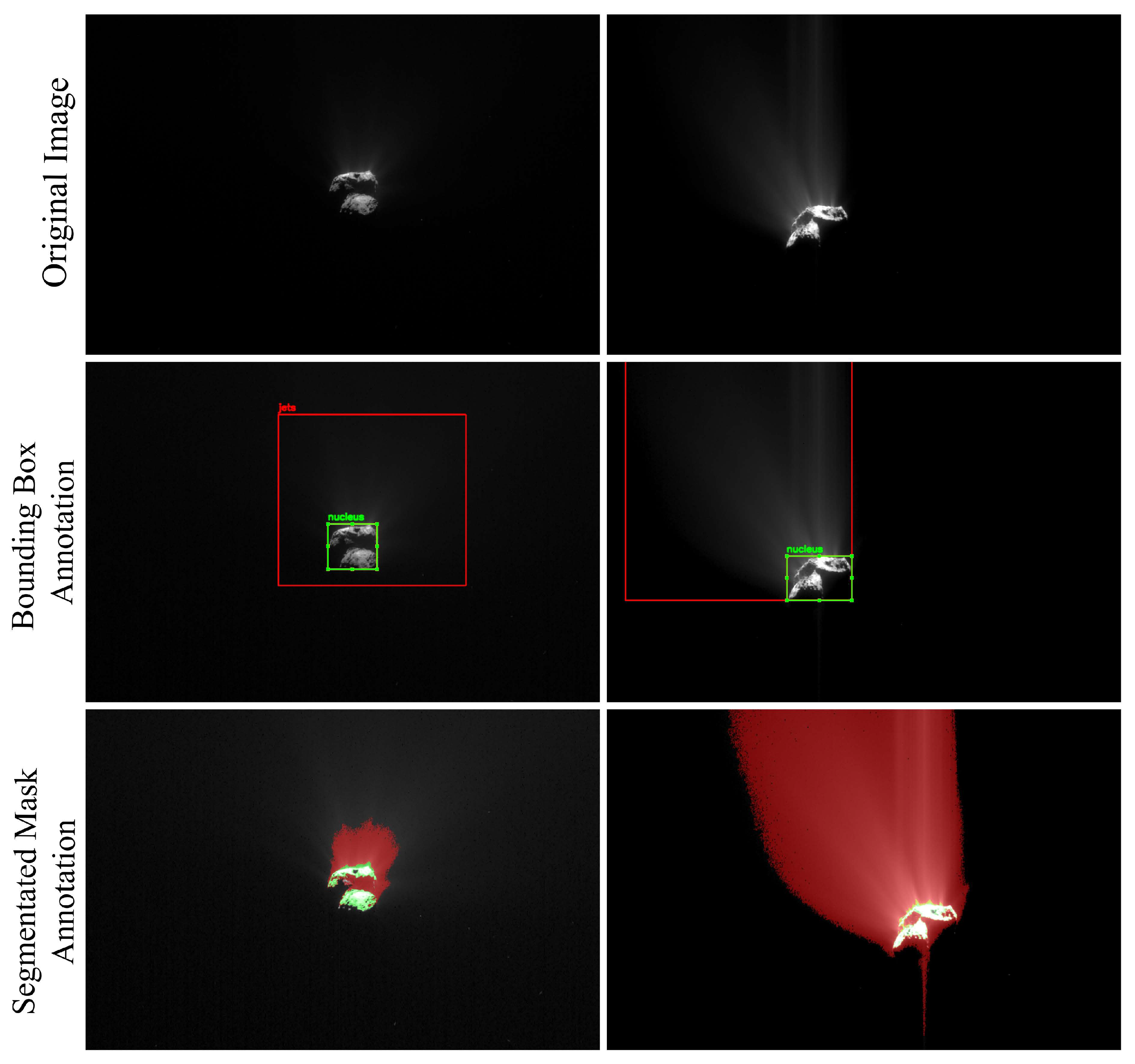
For segmentation annotation, a similar interactive OpenCV-based tool was developed to efficiently generate pixel-level masks for the nucleus and dust jets. The tool provides a simplified interface in which class-specific intensity band-pass thresholds can be adjusted using sliders, with real-time colour overlays displayed alongside the original image to facilitate rapid qualitative validation. A small connected component filter is applied to suppress spurious noise sources such as background stars. The resulting annotations are stored in a unified dataset format comprising normalised images (1 × height × width) and two-channel segmentation masks (2 × height × width), ensuring consistency and seamless integration with downstream evaluation pipelines. Figure 2 shows a small sample of images from the Rosetta dataset together with the corresponding implemented annotations, including bounding boxes and pixel-wise segmentation masks.

These annotations are used exclusively for quantitative evaluation of model performance on real data and are not employed during network training, which is conducted solely on the synthetically generated datasets produced using the FlyByGen tool version 1.0.0. As such, uncertainties in manual annotation primarily affect the reliability of the reported evaluation metrics rather than the learned model parameters.

2.4. Dataset Augmentation

Due to the minimal base dataset, extensive augmentation is applied. The reason for this is twofold. Firstly, a dataset with varied comet positions, rotation, scales, and brightness would have drastically increased the dataset size, while not providing any information which could not be added during preprocessing. With augmentation, the dataset is smaller, but it still yields a more general dataset than a larger dataset with varied scales, etc. Secondly, the network generalises better with more varied augmentation. Specifically, it enables easy scalability of the task complexity. For example, tasks with different object brightnesses or sizes can be easily tested. The following sections introduce the augmentations implemented in this work and the combinations in which they were applied.

2.4.1. Position

As the object is at the centre of the FoV, augmentation is required. In this application scenario, the object may be anywhere in the image, or only partly in the FoV. During augmentation, the object is moved to a random position in the image.

2.4.2. Rotation

During data generation, the camera is rotated around the object to ensure different camera-to-light-source settings. Additionally, the random objects are adapted and stretched into different directions during generation. However, this does not necessarily include rotation of the object. To ensure more randomness in the perception of the target object, the image is rotated randomly around the centre.

2.4.3. Flip

As the rotation does not include mirroring of the object, this was also included as the flip augmentation. An image was flipped horizontally and vertically with a 50% chance.

2.4.4. Scale

The images of FlyByGen are always rendered from the same distance. Generally, in a way that ensures sufficient resolution of the nucleus, but also includes the full dust jets. As this would only allow handling a limited range of object sizes and observation distances, scaling was applied to the image, increasing or decreasing the object’s size within the FoV. The scaling applied in this work was randomly selected from 2.0 to 0.5, meaning the size was either doubled or halved.

2.4.5. Brightness

To simulate different exposure settings, as well as albedo and other brightness-related factors, brightness augmentation was implemented by multiplying the entire image’s pixel values by a single value. The factor ranged from 0.5 to 1.5, and pixels that would thus exceed the image’s maximum value were clipped to the maximum value.

2.4.6. Blur

In realistic observation scenarios, image quality may be degraded by defocus, motion, or onboard processing effects. To increase robustness against such degradations, a blur augmentation was applied. The augmentation smooths the image using an averaging filter with a randomly selected kernel size. The kernel size is drawn uniformly from a predefined range and enforced to be odd, ensuring symmetric filtering. A kernel size of zero corresponds to no blur, such that not every augmented sample is affected. In this work, kernel sizes ranging from 0 to 7 pixels were used, resulting in mild to moderate blur.

2.4.7. Noise

To reduce the domain gap between idealised synthetic training images and real space-borne observations, a simple yet physically motivated noise augmentation was applied during network training. This augmentation does not model a specific imaging instrument in detail but instead aims to expose the network to common noise sources and artefacts present in optical space imagery. For each training image, a random noise strength is sampled from a uniform range, and the final augmented image is obtained by linearly blending the clean synthetic image with a strongly degraded noisy version. This approach allows the network to observe a continuous range of image qualities, from near-ideal synthetic data to heavily degraded samples.

Noise is applied directly to single-channel images, consistent with the input format of the trained networks. The noisy realisation combines several complementary components representative of common noise sources and artefacts observed in optical space imagery. Signal-dependent photon shot noise is introduced to model fluctuations arising from photon counting under low-light conditions. Additive Gaussian noise is applied to approximate electronic read noise. In addition, low-frequency row- and column-wise bias patterns are added to emulate structured artefacts such as residual banding or bias offsets that may remain after imperfect sensor calibration. A spatially correlated multiplicative gain field is further applied to represent photo-response non-uniformity and residual flat-field errors.

To avoid training on unrealistically clean backgrounds, sparse star-like sources are also added as “background clutter”. These sources are generated by randomly placing point-like impulses and smoothing them with Gaussian kernels to approximate a simplified optical point spread function with a faint halo. Finally, a small number of hot and cold pixels are introduced to represent defective or radiation-affected pixels commonly encountered in space imaging systems.

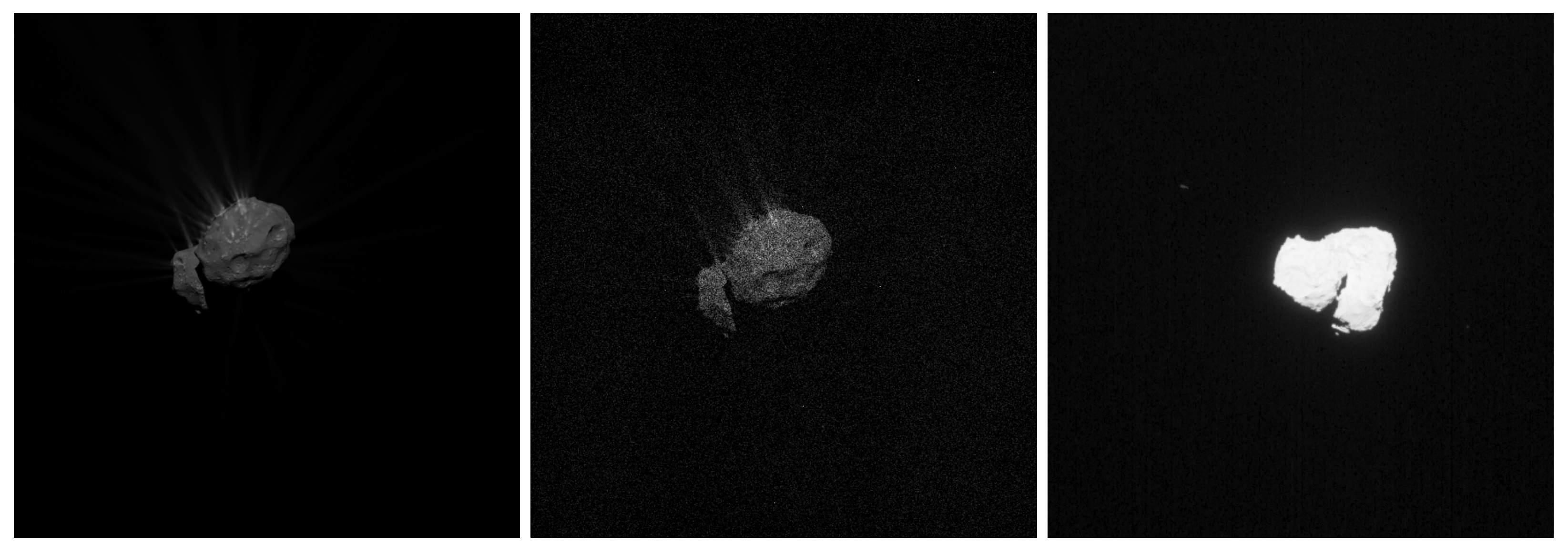
All noise-augmented images are clipped to the normalised intensity range. This strategy introduces realistic sensor noise, structured artefacts, and astronomical background clutter in a controlled and interpretable manner, aiming to improve the robustness of models trained on synthetic comet images when applied to real space-borne data. Figure 3 shows a side-by-side comparison between an image from the Comet dataset, the corresponding noise-augmented image, and an image from the Rosetta dataset with comparable noise characteristics.

From a mission perspective, these noise components correspond to dominant effects encountered in deep-space optical imaging, including photon-limited signal acquisition under low illumination, electronic read noise, residual bias structures after in-flight calibration, and background star fields. Sensitivity of the models to noise variations is therefore expected, as the detectability of small or low-contrast targets, such as cometary dust jets, is inherently constrained by the signal-to-noise ratio. The adopted augmentation strategy exposes the networks to a controlled range of degradations representative of plausible space-borne conditions, allowing the impact of increasing noise severity on detection and segmentation reliability to be assessed.

Overall, this augmentation strategy captures first-order noise processes that dominate performance in optical space imaging and therefore provides a reasonable stress test for assessing robustness under mission-relevant conditions. Each noise component is implemented using standard first-order abstractions commonly employed in space-imaging simulations (e.g., Poisson-distributed shot noise and additive Gaussian read noise), without introducing instrument-specific parametrisation.

2.5. Baseline Data Reduction Methodology

As pointed out previously, data reduction methodologies are mostly still in development, and very few examples are currently in space and operational. Specifically in exploration missions this is still rare. However, the OPIC instrument onboard ESA’s Comet Interceptor mission performs data reduction in certain phases of its mission timeline by cropping the nucleus out of the image to reduce its data budget while sending images of the comet’s nucleus back at an increased rate. OPIC implements a non-CNN blob detector Image Prioritisation (IMPRIO) algorithm developed by Bitlake Technologies as described in [40,41], running on a ProASIC 3 FPGA within OPIC’s camera head. Our team developed our own implementation based on publicly available data. While we had access to the actual reference scripts from Bitlake, we could not use them for this article for intellectual property restrictions. After all, this is an important comparison, as CNN approaches are only justifiable if they considerably outperform existing methods in the sense of power assumption and or data reduction accuracy. The algorithm was run on the test dataset and the real world data to enable quantitative and qualitative comparison. In addition to the more complex IMPRIO-inspired implementation, we also used a simpler thresholding and blob detection-based code, based on OpenCV [42].

2.5.1. IMPRIO-Inspired Implementation

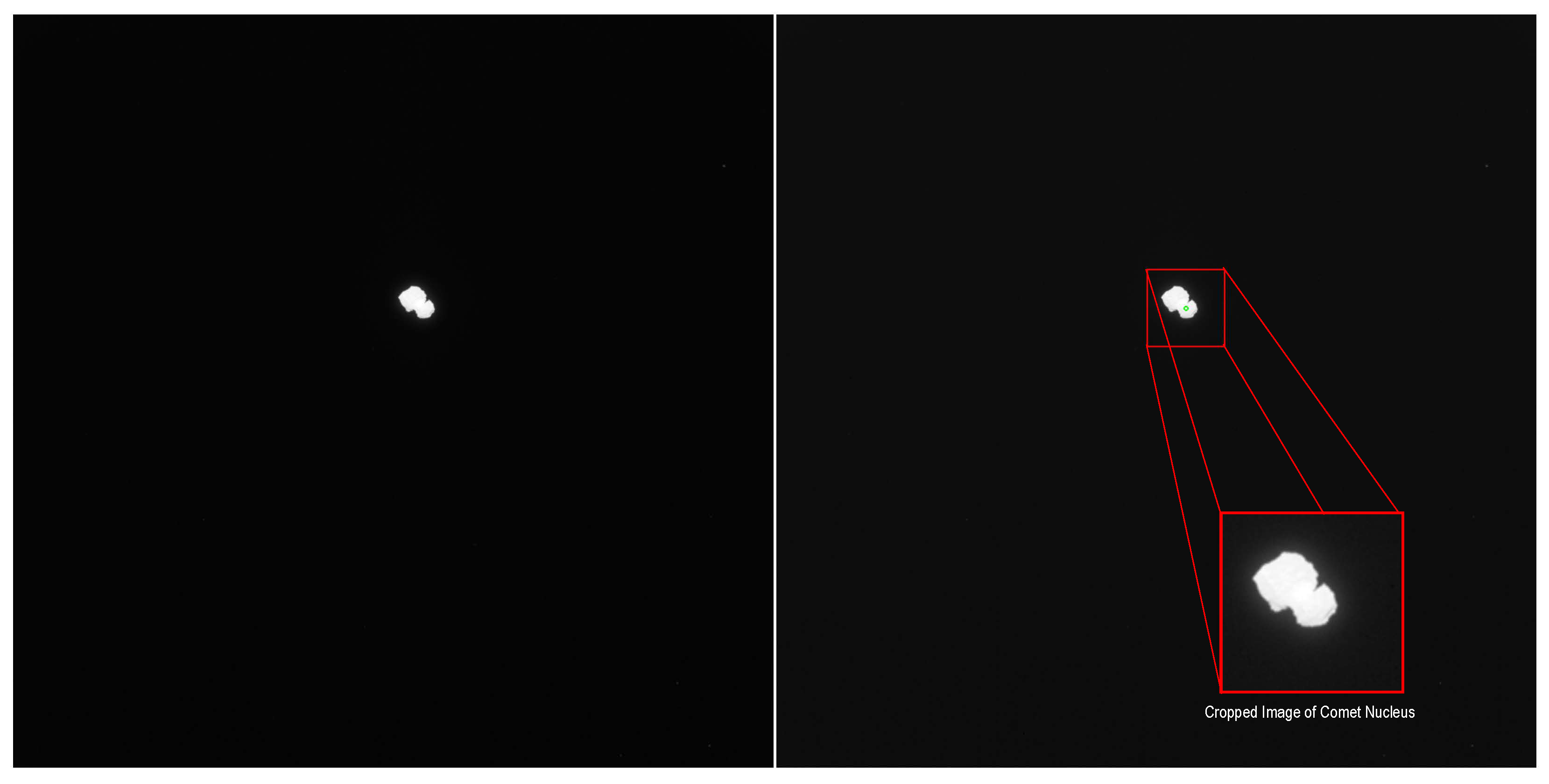
The IMPRIO algorithm performs deterministic image prioritisation using a low-complexity, multi-scale spatial filtering approach. Input images are first intensity-quantised to a small number of discrete levels and analysed across a scale pyramid constructed via successive 2 × 2 binning. At each pyramid level, a discrete Laplacian-of-Gaussian-like filter is applied in a sliding-window fashion, and the spatial location and scale yielding the maximum absolute filter response are selected as the most salient feature. This location is mapped back to full resolution and used to extract a fixed-size region of interest for prioritised downlink. Figure 4 shows the output of the IMPRIO-inspired implementation on a sample image from the Rosetta dataset, illustrating the detected comet and the corresponding bounding box used for image cropping as part of the data reduction process.

A key limitation of this approach is that the crop window size is fixed at configuration time and does not adapt to object extent or scene content. To account for this constraint in evaluation, a logarithmic sweep of window sizes was performed, allowing the identification of window dimensions that best match the test data while maintaining the algorithm’s non-adaptive nature.

2.5.2. OpenCV-Based Blob Detector

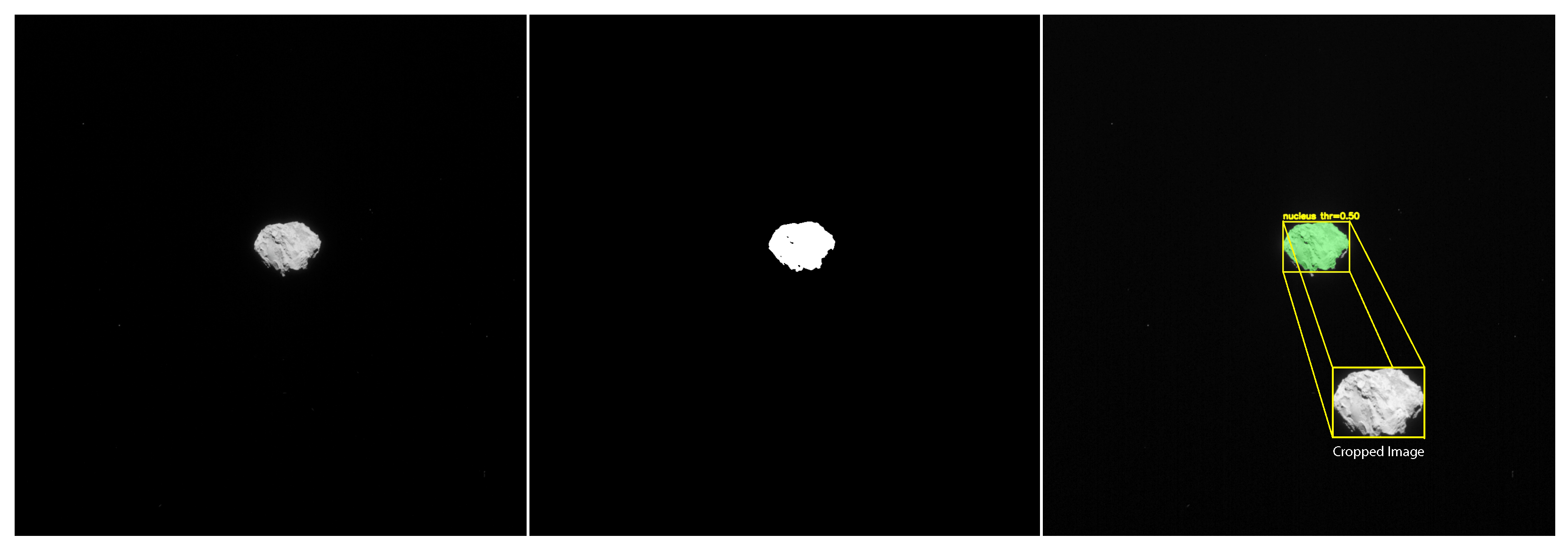
A classical image-processing baseline was implemented using OpenCV to provide a non-learning reference for nucleus segmentation. Each input image was converted to greyscale and binarised using Otsu’s global thresholding method [43], which determines an optimal threshold by maximising inter-class variance. Connected component analysis was then applied to the binary image, and the largest foreground component was selected as the detected blob, corresponding to the comet nucleus. The resulting binary mask was used as a baseline for comparison with the CNNs. This method was evaluated using bounding box-based metric analysis for detection tasks and pixel-wise metrics for segmentation tasks (Intersection over Union, Dice coefficient). Figure 5 shows the output of the simple OpenCV-based blob detector implemented on a sample image from the Rosetta dataset.

2.6. CNN Semantic Segmentation

Semantic segmentation enables pixel-level selection of scientifically relevant regions and therefore represents the theoretical upper bound for achievable onboard data reduction. By transmitting only pixels classified as relevant, segmentation-based approaches can, in principle, eliminate all background data.

In practice, semantic segmentation is computationally demanding and sensitive to dataset characteristics. In the considered cometary imagery, pixels may simultaneously belong to multiple semantic categories (e.g., nucleus and dust jets). Consequently, a multi-hot segmentation formulation is adopted, where each pixel may be assigned to multiple classes. An explicit background class was evaluated but discarded, as it consistently reduced performance due to class imbalance without providing additional benefit for the data reduction task.

Multiple segmentation architectures were evaluated to span a broad range of accuracy–complexity trade-offs, from lightweight mobile-oriented models to high-capacity multi-scale networks. The selected architectures are representative of state-of-the-art approaches in general semantic segmentation as well as models previously adopted in space-related imaging applications. No architectural modifications were introduced outside of the input format to enable greyscale input and output format for multi-hot tasks. All networks were used as described in the respective references.

Table 1. Semantic segmentation networks used in this work. U-Net Custom dx fy, where dx is depth and fy is the initial filter. The terms MobileNetV3, Resnet50, Resnet101 always refer to the implemented backend; Params refer to the number of network parameters; and Tera Operation Per Second (TOPS) describes the computational complexity.

Architecture	Short Name	Params	TOPS
U-Net Custom d3 f16	UNET_3_16	484,866	0.0747
U-Net Custom d3 f32	UNET_3_32	1,947,010	0.0975
U-Net Custom d3 f64	UNET_3_64	7,787,650	0.1204
U-Net Custom d4 f16	UNET_4_16	1,931,266	0.2959
U-Net Custom d4 f32	UNET_4_32	7,771,906	0.3872
U-Net Custom d4 f64	UNET_4_64	31,118,594	0.4785
U-Net Custom d5 f16	UNET_5_16	7,708,674	1.1781
U-Net Custom d5 f32	UNET_5_32	31,055,362	1.5433
U-Net Custom d5 f64	UNET_5_64	124,410,370	1.9084
LR-ASPP	LRASPP	3,218,020	0.0165
DeepLabv3 MobileNetv3	Deeplabv3_mnv3	11,024,157	0.0795
DeepLabv3 Resnet50	Deeplabv3_res50	41,992,919	1.3872
DeepLabv3 Resnet101	Deeplabv3_res101	60,985,047	2.0112
FCN Resnet50	FCN_res50	35,306,199	1.1851
FCN Resnet101	FCN_res101	54,298,327	1.8092

summarises the segmentation networks considered in this work, including their primary motivation, parameter count, and estimated computational complexity. These metrics are later used to assess segmentation performance as a function of onboard resource requirements. We note that the U-Net networks are custom implemented to allow accuracy scaling with network complexity.

2.6.1. Fully Connected Network

FCN [44] is the first fully convolutional network for semantic segmentation. The premise for this architecture is to utilise convolutional layers to enable dense, pixel-wise predictions. It is an encoder feature extractor, while the decoder upsamples with transpose convolutions. The skip architecture allows for detailed refinements. It is a quite simple architecture that provides a good baseline and is mostly relevant due to its historical significance. The network efficiency is not high, and only ResNet50 and ResNet101 backbones are included in this study, providing a strong baseline with more than sufficient model capacity.

2.6.2. LR-ASPP

The Lite Reduced Atrous Spatial Pyramid Pooling (LR-ASPP) [45] model is the result of the semantic segmentation development of the MobileNetV3 developers. The goal of this development was to create an efficient segmentation architecture for mobile and embedded systems. The convolutions here are depth-wise separable based on MobileNetv3, which is combined with a lightweight Lite Reduced Atrous Spatial Pyramid Pooling (ASPP) head [46]. This is as highly relevant a network as it is specifically targeted for low-power and compute applications.

It should be noted that this network was specifically created for embedded systems; the following segmentation networks are not. Thus, only one variant of this network is included in this work, and this is the original MobileNetV3 variant.

2.6.3. U-Net

This architecture was originally developed for biomedical image segmentation for small datasets [47]. The premise of this architecture is its symmetry of encoder and decoder with an additional strong skip connection to each level. As it is specifically well suited for small datasets and irregular structures, it has become widely adopted for space applications [16,17]. In this work, various parameter combinations have been tested from filter sizes between 16 and 64 to network depths between 3 and 5. This also created various network sizes.

2.6.4. Deeplabv3

The DeepLabV3 model is based on the Rethinking Atrous Convolution for Semantic Image Segmentation paper [46]. It has three commonly used backbones, such as MobileNetV3, ResNet50, and ResNet101.

2.7. CNN Object Detection

Object detection was evaluated as the second data reduction strategy. Unlike segmentation, detection-based approaches select rectangular regions enclosing target objects, resulting in less precise spatial selection but significantly reduced computational complexity. In this work, the use of detection methods aims to provide a trade-off between data reduction efficiency and onboard feasibility.

In the considered application scenario, it is assumed that at most one cometary object is present in the field of view. To avoid the risk of discarding relevant data, confidence-based filtering was not applied; instead, the highest-scoring detection was always selected. This reflects an operationally conservative strategy suitable for autonomous onboard processing.

A diverse set of detection architectures was selected to cover different detection paradigms (two-stage, one-stage, anchor-based, anchor-free) and a wide range of computational requirements. The YOLOv11 family was included in multiple sizes to explicitly explore the accuracy–complexity spectrum. All models were used without architectural modification.

An overview of the evaluated detection networks is provided in

Table 2. Object detection networks used in this work. The terms MobileNetV3, vgg16, and Resnet50 refer to the implemented backends; Params refer to the number of network parameters; and TOPS describes the computational complexity.

Architecture	Short Name	Params	TOPS
Faster R-CNN MobileNetV3 large 320 FPN	FRCNN_mnv3_320	18,935,354	0.0029
Faster R-CNN MobileNetV3 large FPN	FRCNN_mnv3	18,935,354	0.0164
Faster R-CNN Resnet50 FPN	FRCNN_res50	41,304,286	0.2679
Faster R-CNN resnet50 FPN v2	FRCNN_res50_v2	43,261,278	0.4044
FCOS Resnet50 FPN	FCOS_res50	32,066,760	0.2510
Retinanet Resnet50 FPN	Retina_res50	32,189,439	0.2544
Retinanet Resnet50 FPN v2	Retina_res50_v2	36,373,375	0.2569
SSD 300 vgg16	SSD_vgg16	23,879,570	0.0610
SSD Lite MobilNetv3 large 320	SSD_lite_mnv3	3,725,420	0.0011
YOLO11 detection size n	YOLO11_n	2,590,230	0.0165
YOLO11 detection size s	YOLO11_s	9,428,566	0.0552
YOLO11 detection size m	YOLO11_m	20,054,550	0.1746
YOLO11 detection size l	YOLO11_l	25,312,022	0.2234
YOLO11 detection size x	YOLO11_x	56,876,086	0.5004
YOLOv4-tiny	YOLOv4-tiny	6,056,606	0.0422

.

2.7.1. Faster Region-Based Convolutional Neural Networks

The Faster Region-based Convolutional Neural Networks (R-CNN) model is based on the “Faster R-CNN: Towards Real-Time Object Detection with Region Proposal Networks” paper [48]. It is a two-stage detector that first generates proposals using a region proposal network and then classifies and refines bounding boxes for these proposals. It is expected to provide high detection accuracy at the cost of higher complexity and latency.

2.7.2. RetinaNet

The RetinaNet model is based on the “Focal Loss for Dense Object Detection” paper [49]. It is a one-stage detector intended to bridge the gap in accuracy with two-stage methods by implementing focal loss between foreground and background during training. It is expected to prioritise speed over accuracy.

2.7.3. Fully Convolutional One-Stage

The Fully Convolutional One-Stage Object Detection(FCOS) model is based on the “FCOS: Fully Convolutional One-Stage Object Detection” paper [50]. It is an one-stage detector that predicts object locations without anchors on each pixel, avoiding anchor engineering.

2.7.4. Single Shot MultiBox Object Detector

The SSDLite model is Single Shot MultiBox Object Detector (SSD) based on the “SSD: Single Shot MultiBox Detector” [51] and “Searching for MobileNetV3” [45]. It is a SSD that predicts bounding boxes in a single forward pass using anchors. It is optimised for easy deployment and low latency.

2.7.5. You Only Look Once

YOLO 11 [52] is a modern YOLO version, which aims real-time performance with strong accuracy. Detection is performed in a single pass, is highly optimised for both training and inference, and is expected to offer a very good speed–accuracy trade-off. Unlike earlier YOLO versions, it is also anchor free.

YOLOv4-tiny [27] is included here as a detailed reference [26] of an onboard deployment. Relevant here is that it is not included in the training and evaluation process, but rather as an example of network complexity deployed in space.

2.7.6. Feature Pyramid Network

Several evaluated detection architectures incorporate Feature Pyramid Network (FPN), which enables multi-scale feature aggregation and improves robustness to object size variation [53]. This is particularly relevant for cometary imagery, where nuclei and dust features may appear at significantly different spatial scales. The presence of an FPN is explicitly indicated in model names and tables where applicable.

2.8. Training Strategy

For this study, two training runs were performed for all architectures: one with noise and blur augmentations deactivated, creating a baseline network for ideal mission conditions, assuming an “ideal” camera, and the second training run which was performed with blur and noise augmentation activated. This is aimed at enabling a more generalised training run. How well this training generalises to real data is highly relevant for this study.

Besides the training augmentation settings, the two runs had exactly the same setup. A hyperparameter search was used to determine a near-optimal network performance. Training was conducted on an in-house machine learning server with 4 NVIDIA RTX A6000 Graphical Processing Unit (GPU) and an Intel Xeon Gold 6426Y Central Processing Unit (CPU), using both PyTorch 2.6.0 and TensorFlow 2.19 backends, with Ray Tune 2.52 employed for hyperparameter optimisation. The search space included:

• Number epochs: 30;
• Batch size: {16, 32, 64};
• Loss function: CrossEntropyLoss (training and evaluation);
• Optimiser: Adam;
• Learning rate: {1 $\times {10}^{-4}$, 1 $\times {10}^{-3}$};
• beta1: {0.85, 0.95};
• Momentum: {0.8, 0.99};
• Learning Rate scheduler: monitored on avg loss, reduction factor 0.5, mode min, patience 2.

An initial wide search was conducted, after which non-promising parameter ranges were discarded, narrowing the search space. Ultimately, seven runs were completed for each architecture on the final above-defined search space, trained for up to 30 epochs. For each run, the epoch achieving the highest validation score was selected for deployment.

Lastly, for the semantic segmentation task, a sigmoid threshold sweep was performed to determine an independent activation threshold for each class. This sweep was performed on the validation set after the training was completed. During training, a threshold of 0.5 was used.

2.9. Evaluation Aspects

The evaluation strategy for this work is designed to assess neural networks for their suitability for reliable onboard data selection rather than maximising segmentation or detection accuracy in isolation. Consequently, multiple complementary evaluation aspects are considered, reflecting both scientific relevance and operational constraints.

The evaluation focuses on three main aspects:

• the accuracy of cometary object detection and segmentation,
• the effectiveness of data reduction achieved through network-based selection,
• the computational complexity associated with different network architectures.

Together, these aspects enable a comprehensive assessment of the trade-off between information retention, bandwidth reduction, and deployability.

2.9.1. Network Evaluation Metrics

The primary evaluation metric for both detection and segmentation tasks is the Dice coefficient [54], which provides a robust measure of overlap between predicted regions and ground-truth masks. Dice is particularly well suited for this application, as it emphasises the correct identification of relevant regions while being less sensitive to class imbalance.

In addition to the Dice coefficient, for segmentation, class-specific precision and recall values are reported to distinguish between over-selection and under-selection of relevant regions. For comparability with established computer vision benchmarks, average Intersection over Union (IoU) [55], Common Objects in Context mean Average Precision (COCO mAP) [56], and PASCAL Visual Object Classe (VOC) Average Precision (AP) [57] at an (IoU) threshold of 0.5 are also computed. While the aim of this work is not to achieve state-of-the-art accuracy, these metrics enable contextualization of the results with respect to existing approaches. Most importantly for this work is the average Dice coefficient for determining the detection accuracy. In addition, the PASCAL VOC AP at 0.5 (VOC AP@0.5) is used as a reliability measure to determine whether an object was detected precisely enough. The premise here is that the higher the precision, the higher the reliability, and the fewer total misses are among the predictions.

Due to the nature of the application scenario, it is assumed that at most one comet is present within the field of view of each image. Consequently, confidence thresholding is discarded for object detection networks to ensure that a prediction is always generated and that no potentially relevant data are unnecessarily omitted.

2.9.2. Data Reduction Metrics

Data reduction performance is quantified by the fraction of image data selected for simulated downlink by the proposed models. For segmentation-based approaches, this fraction corresponds to the number of pixels classified as relevant by the predicted segmentation masks. For detection-based approaches, the selected data volume is defined by the pixel area enclosed within the predicted bounding boxes.

The selected data volume is normalised by the total image size to obtain a reduction ratio directly comparable across methods. When evaluated jointly with the Dice coefficient, this formulation enables an intuitive assessment of the trade-off between retained scientifically relevant information and achieved reduction in transmitted data volume, thereby characterising both the efficiency and the fidelity of the data reduction process.

2.9.3. Network Complexity

Network complexity is assessed using theoretical computational cost and model size metrics. The number of parameters and the estimated number of operations in TOPS are used as proxies for onboard computational requirements. These values are obtained using established profiling tools such as ptflops and the TensorFlow profiler. Evaluating performance as a function of network complexity enables an assessment of deployability under realistic onboard processing constraints.

3. Results

3.1. Qualitative Analysis

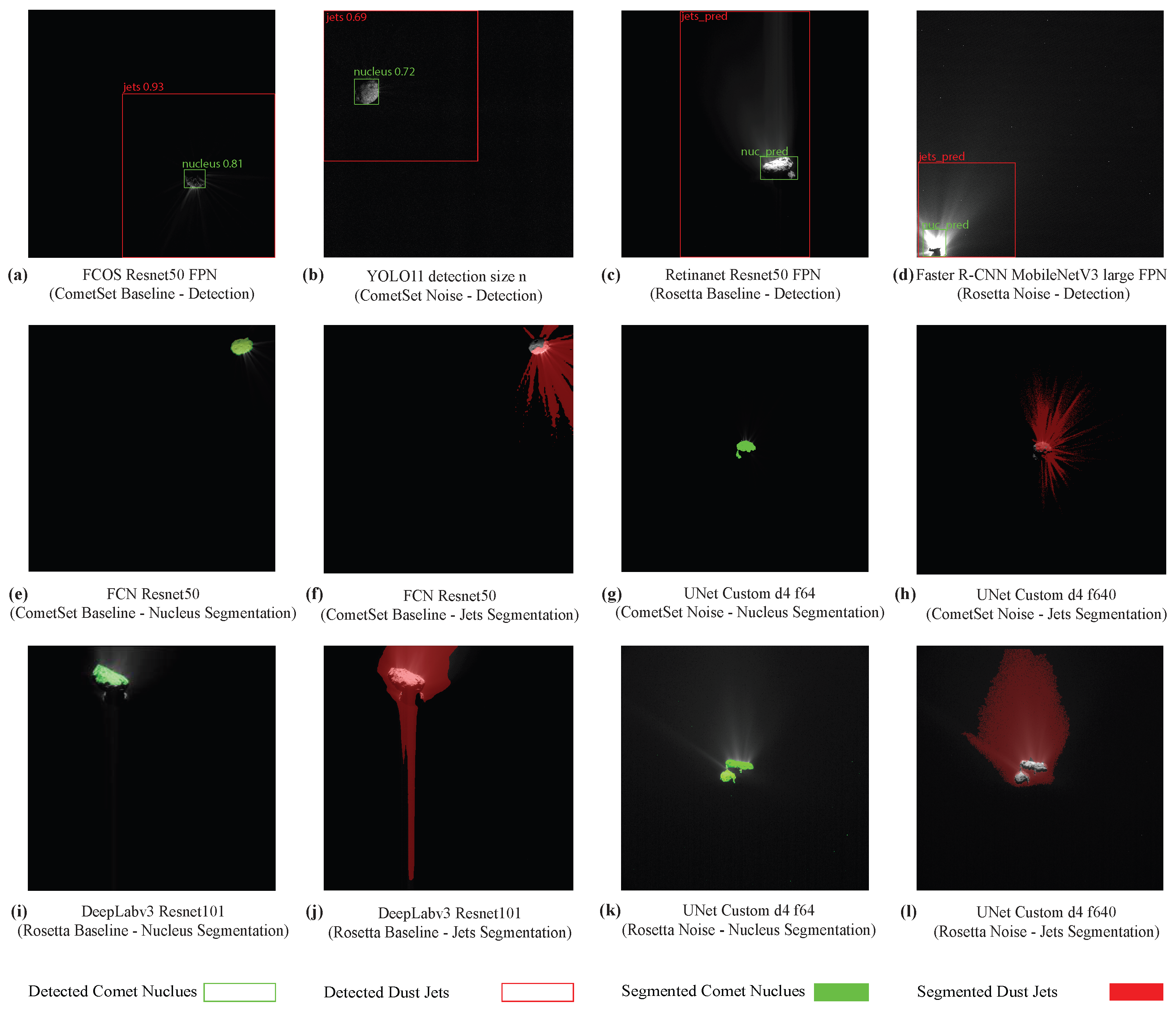
Figure 6 illustrates representative inference outputs from the evaluated detection and segmentation models on both the synthetic CometSet and the Rosetta datasets. The figure provides a qualitative overview of typical prediction behaviour across a subset of baseline and noise-augmented training configurations and highlights differences between detection and segmentation tasks, as well as between nucleus and dust jet classes.

Qualitative inspection of the detection results indicates that comet nucleus localisation is generally robust across the datasets, even in the presence of noise and illumination gradients. Bounding boxes for the nucleus are typically spatially stable and well centred on the target, suggesting that nucleus detection is driven by strong intensity and geometric cues that transfer reliably from synthetic to real imagery. In contrast, dust jet detection exhibits greater variability, with bounding boxes occasionally overextending into background regions or partially covering diffuse jet structures, particularly under low-signal-to-noise ratio conditions.

The segmentation results reveal a more pronounced performance gap between nucleus and dust jet classes. Nucleus segmentation masks are generally compact and spatially coherent, whereas dust jet segmentation remains a challenging task across most architectures. Common qualitative failures observed include fragmented jet masks, incomplete coverage of faint structures, and sensitivity to background noise and star-like clutter. These effects are more prominent in Rosetta images, where real background complexity and subtle intensity gradients can lead to either under-segmentation of faint jets or over-segmentation into surrounding regions.

Models trained with noise-augmented synthetic data exhibit visibly improved qualitative robustness, particularly in maintaining spatially consistent predictions under varying noise conditions. Compared to baseline-trained networks, these models tend to produce smoother segmentation masks and fewer spurious activations in low-signal background regions. Nevertheless, even relatively small mismatches between synthetic and real noise characteristics can still result in noticeable prediction instability, underscoring the inherent difficulty of the task.

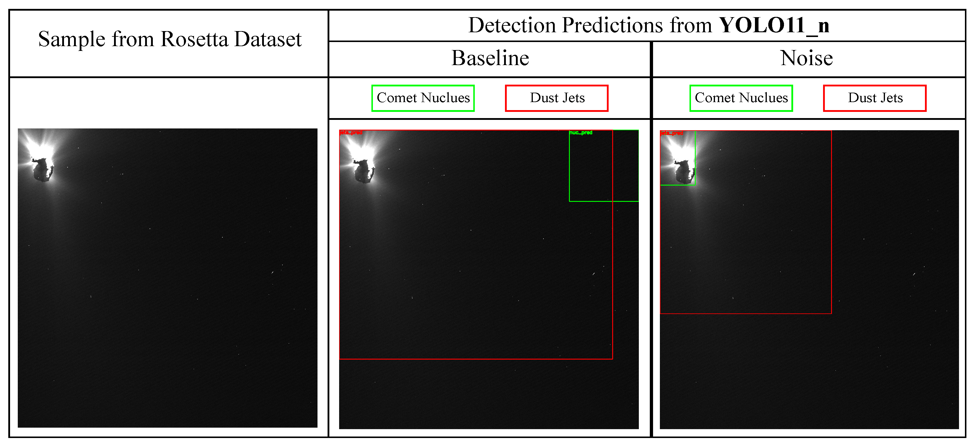
To further illustrate the effect of noise-augmented synthetic training on real mission imagery, Figure 7 presents a direct qualitative comparison of detection outputs from the YOLO11_n model on a particularly noisy Rosetta image. The baseline model produces an overly large dust jet bounding box that extends well beyond the physically plausible region of interest, indicating sensitivity to background noise and star-like clutter. In contrast, the model trained on noise-augmented synthetic data yields more stable detection, even under challenging noise conditions. This example highlights how exposure to realistic noise characteristics during training improves robustness and reduces false activations when applied to spaceborne observations.

It is worth noting that the ability of some segmentation models to produce tight dust-jet masks on both noise-augmented synthetic CometSet images and the Rosetta datasets is a promising qualitative result. Dust jets represent low-contrast, diffuse, and highly variable structures whose appearance depends strongly on illumination geometry, background noise, and viewing conditions. The observed segmentation behaviour indicates that learned models are able to capture meaningful jet morphology rather than responding solely to high-contrast cues. While segmentation errors and instability persist, these results suggest that dust-jet segmentation from synthetic training data is feasible and warrants further investigation.

From a data reduction perspective, these qualitative results are encouraging. Even imperfect detection and segmentation enable selective masking of scientifically relevant regions and aggressive suppression or compression of background pixels. As such, the observed qualitative behaviour supports the feasibility of using learned detection and segmentation models as onboard data reduction tools, provided that their robustness limits and failure modes are well understood.

3.2. Network Accuracy Determination

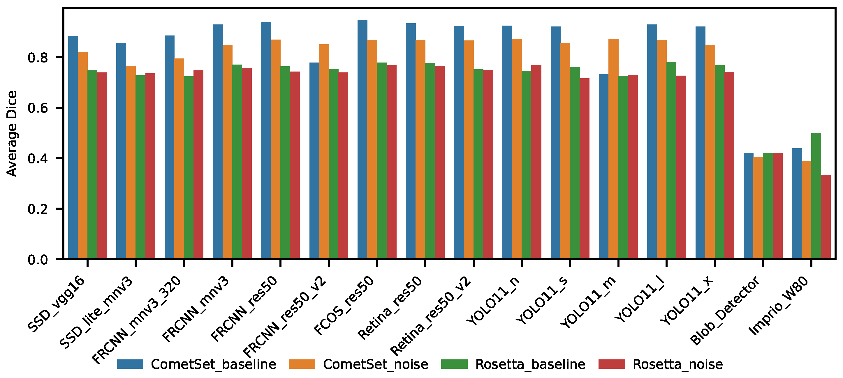
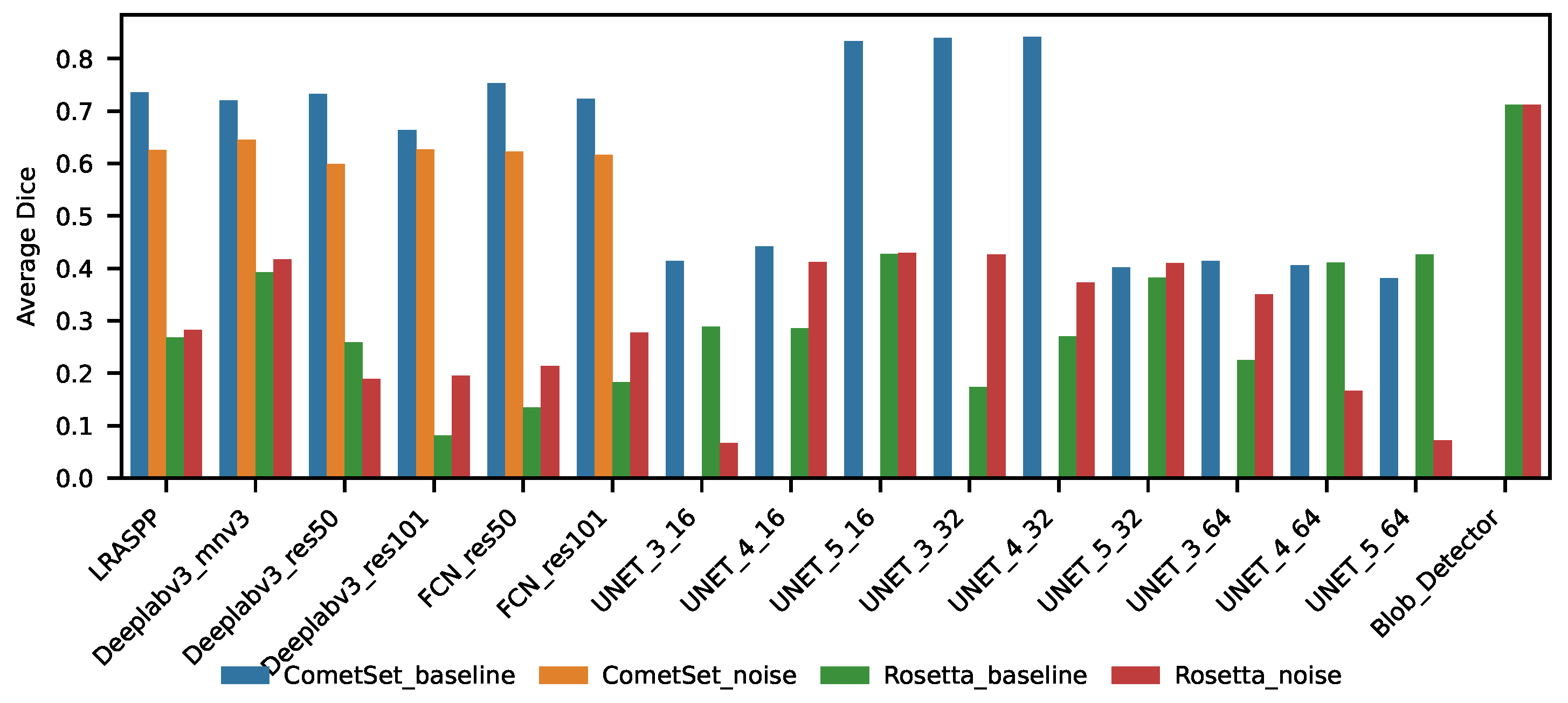
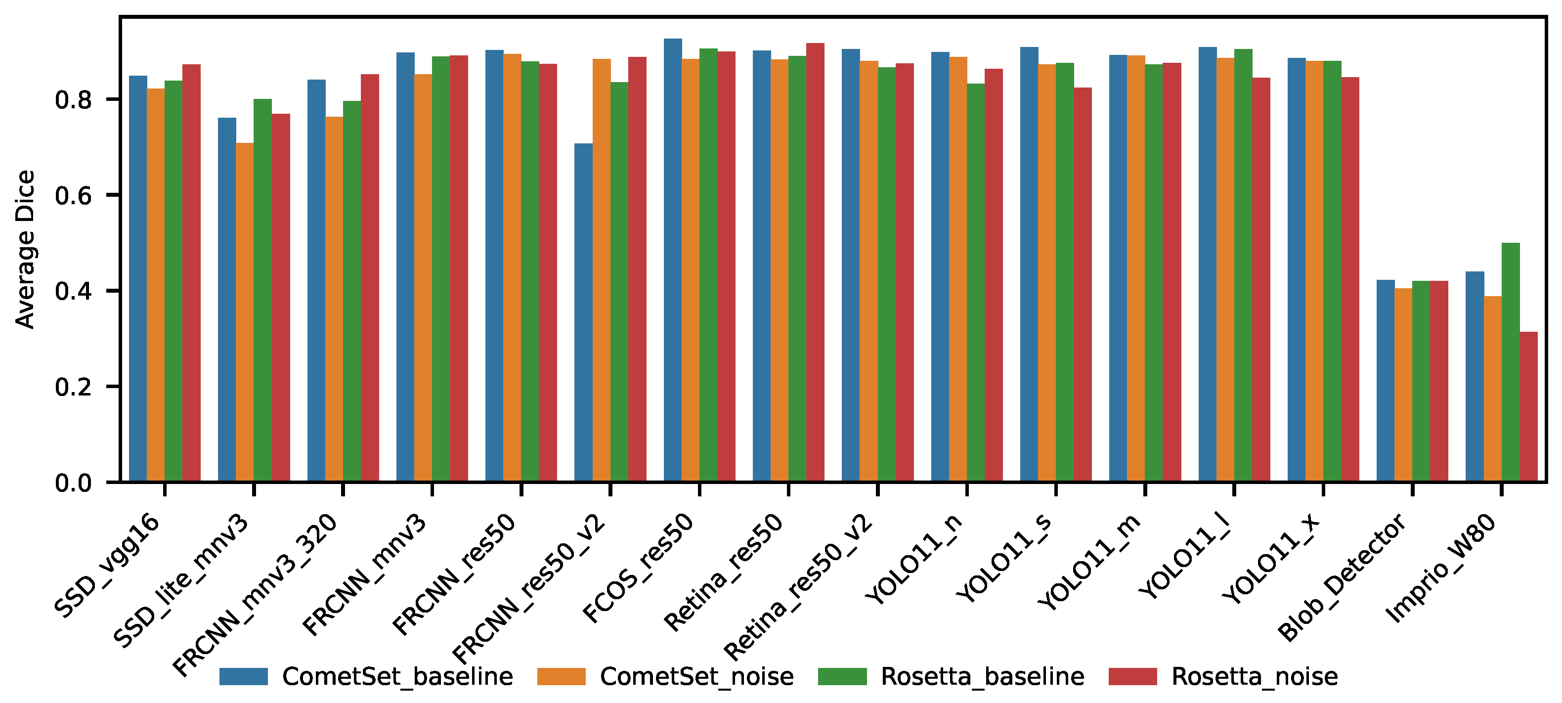
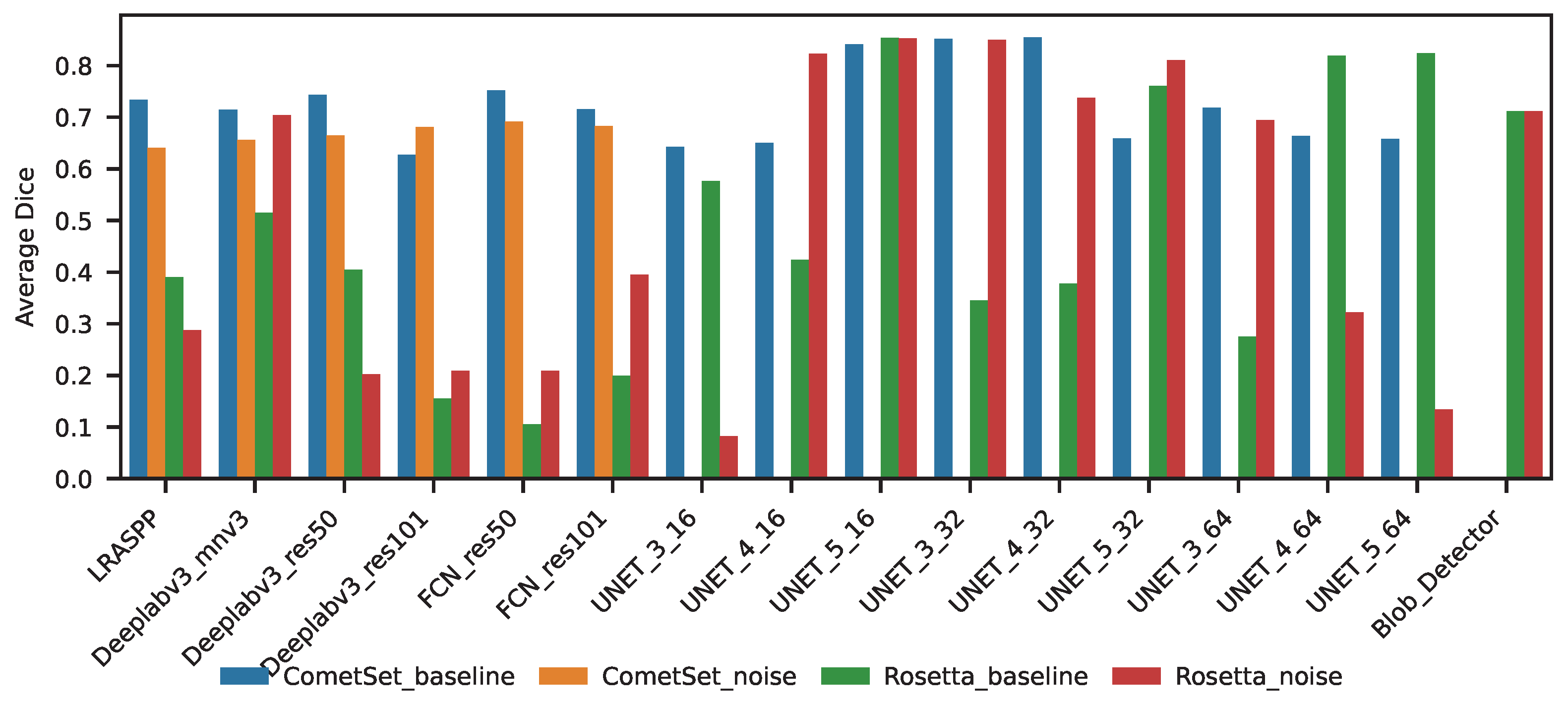
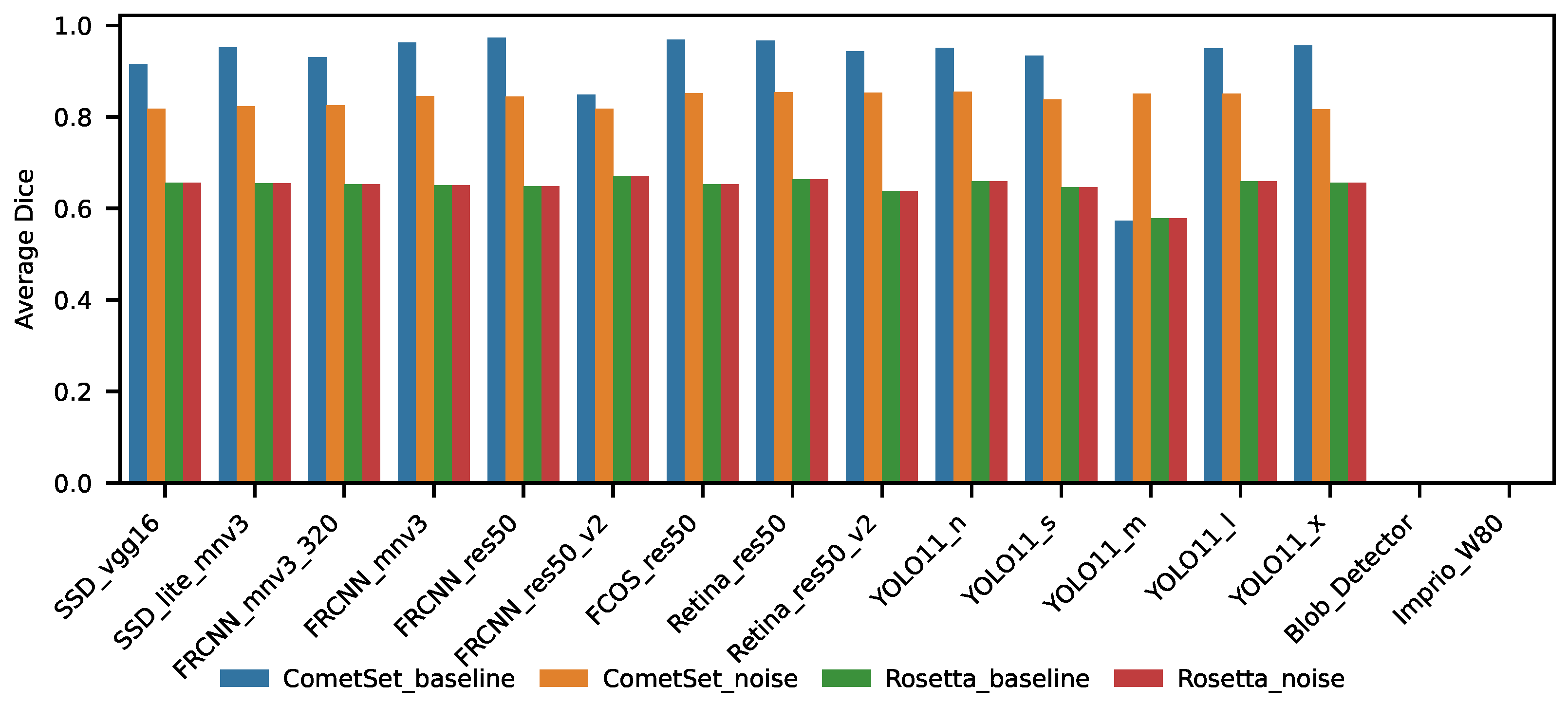
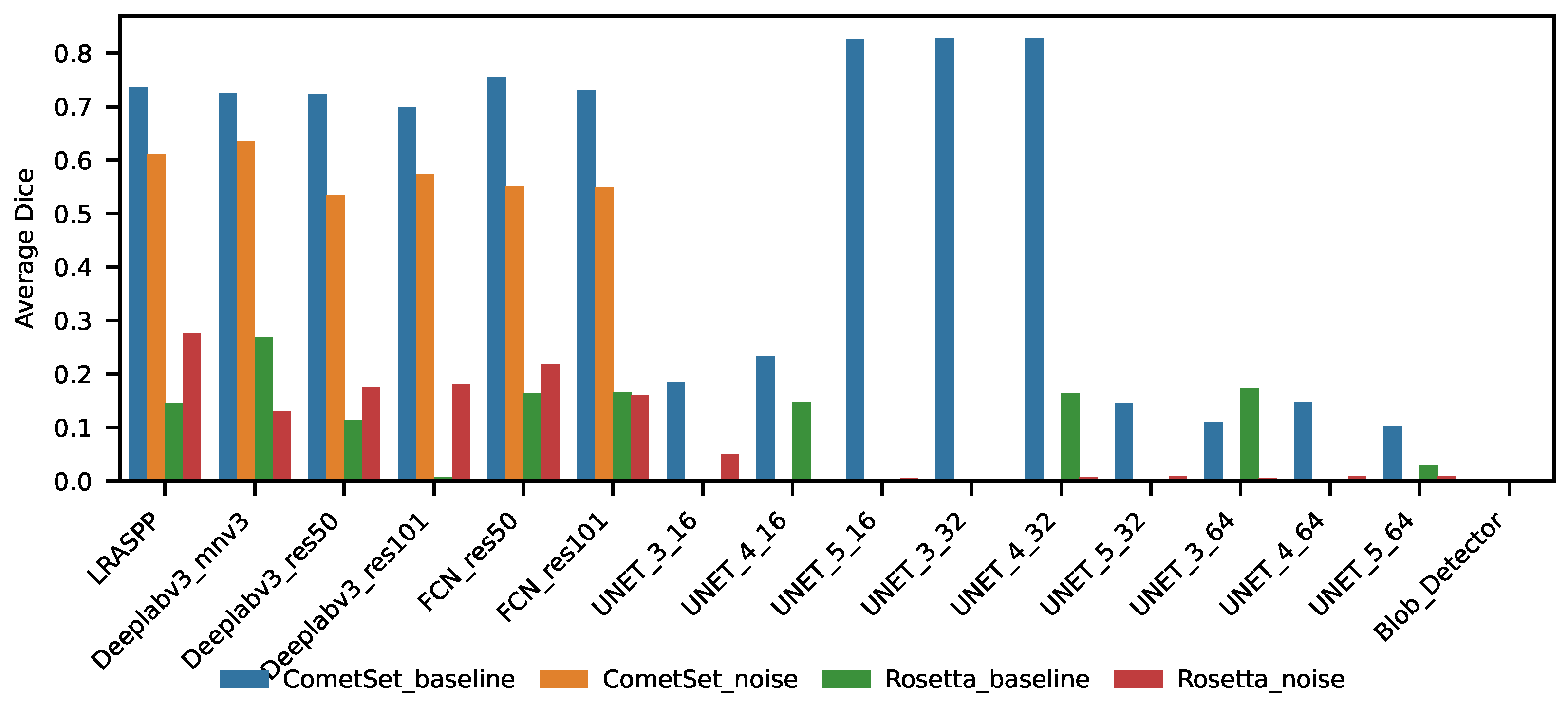
The results of the training and evaluation can be seen in Figure 8, Figure 9, Figure 10, Figure 11, Figure 12 and Figure 13. For this, we selected the Dice coefficient [54]. We plotted separately the performance for the combined nucleus and jets segmentation case, and separate cases for both nucleus and jets. All networks we successfully utilised and trained are shown, together with a simple OpenCV [42] blob detector and an OPIC IMPRIO-inspired algorithm.

The combined case in Figure 8 shows that the networks clearly perform better on the CometSet data, which were used for training. Transferring to the real-world Rosetta dataset results in a significant reduction in accuracy.

The situation changes with considering the case of only detecting the nucleus Figure 10. In this case, the difference between CometSet and Rosetta dataset almost disappears for several network types. The best overall performers are FCOS_res50, FRCNN_mnv3, Retina_res50_v2, and SSD_vgg16. All of these show similar performances and are equally strong for real Rosetta data. During baseline training, two outliers were identified: FRCNN_res50_v2 and YOLO11_m. A detailed investigation of the training logs revealed that during training, a process failed, and the automatic recovery failed to restore the optimiser state, leading to incorrect training continuation.

Additionally, one can see the detector’s performance. The blob detector performed reasonably well given its limitations but was clearly outperformed by all networks. Also, IMPRIO implementation (Imprio_80) performed similarly. Of course, there are no results expected for IMPRIO on the dust jets.

For the segmentation networks, the training remained challenging throughout the project. One can see that the U-Net networks only have relevant baseline results. For example, on noisy data, the U-Net achieved a close to zero average dice coefficient for the jets. On the other hand, some of the U-Net baseline models performed far better than all other networks. With a peak value of 0.84 for the dice coefficient across all classes, the next best non-U-Net(FCN_res50) network achieved at most 0.75 avg_dice. On noisy data, the maximum avg_dice was 0.65 for Deeplabv3_mnv3.

The reasons for the larger differences in segmentation across the entire comet (nucleus + jets) become evident in Figure 12. This shows a large systematic difference between CometSet and Rosetta imagery. One of the main issues here could be the manual annotation process for Rosetta images, as CometSet used segmentation masks co-generated with the images.

3.3. Network Reliability Assessment

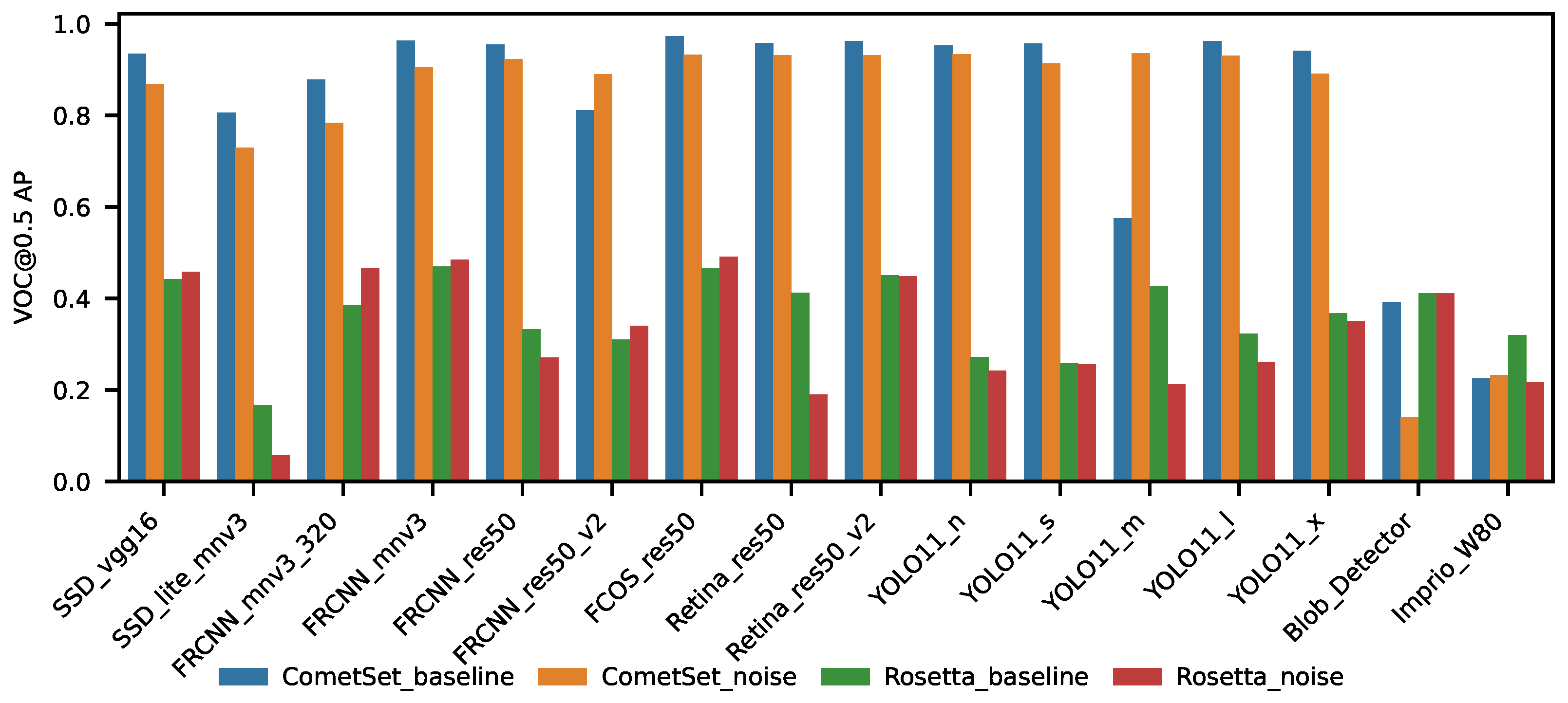
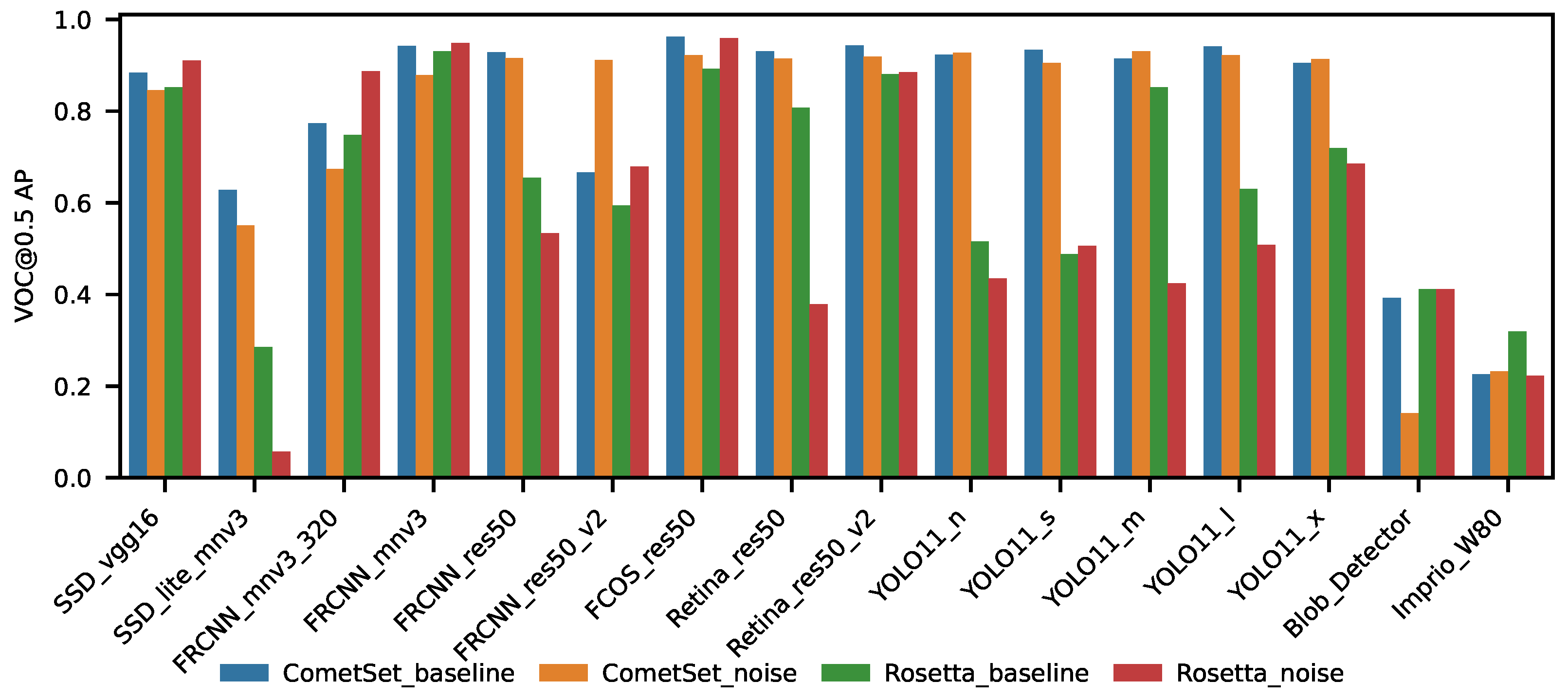
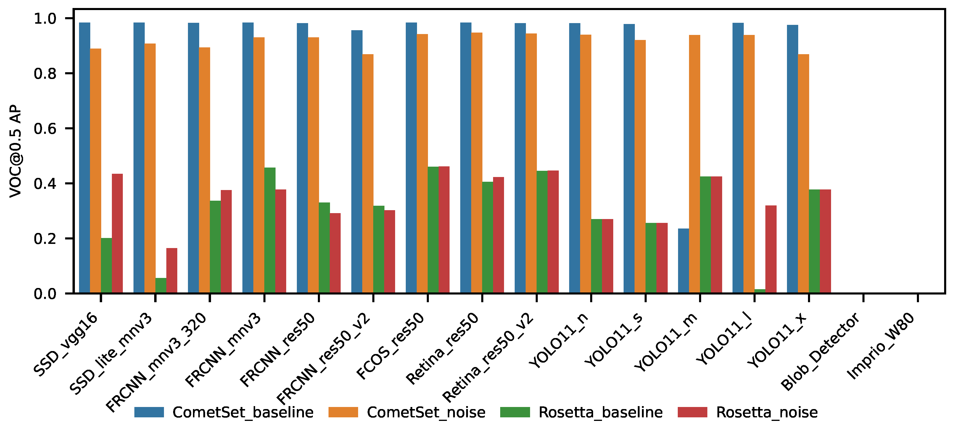
Reliability was assessed by studying the VOC AP@0.5 for each network across each dataset; the corresponding plots are shown in Figure 14, Figure 15 and Figure 16. This metric was only calculated for the detection task. The AP threshold is set to 0.5 IoU, thus providing a metric showing how often an object was not found sufficiently good.

The best performing network across all classes is FCOS_res50. Notably, the precision drop in jet detection on the Rosetta dataset is very high, primarily because manually annotating the data is more challenging than synthetic annotation. The nucleus precision is much better, but still a significant drop is seen for most networks between the CometSet and Rosetta data.

3.4. Achieved Data Reduction

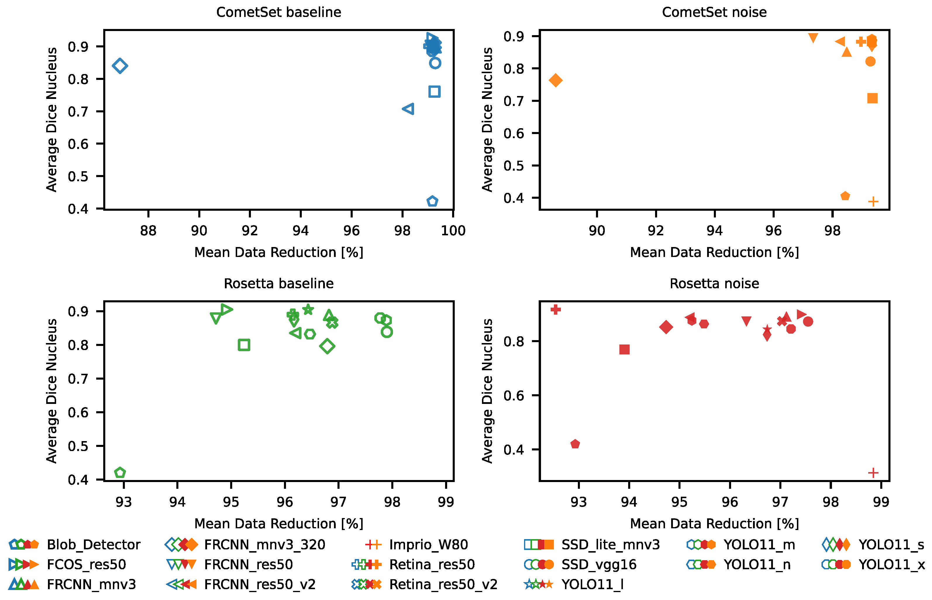
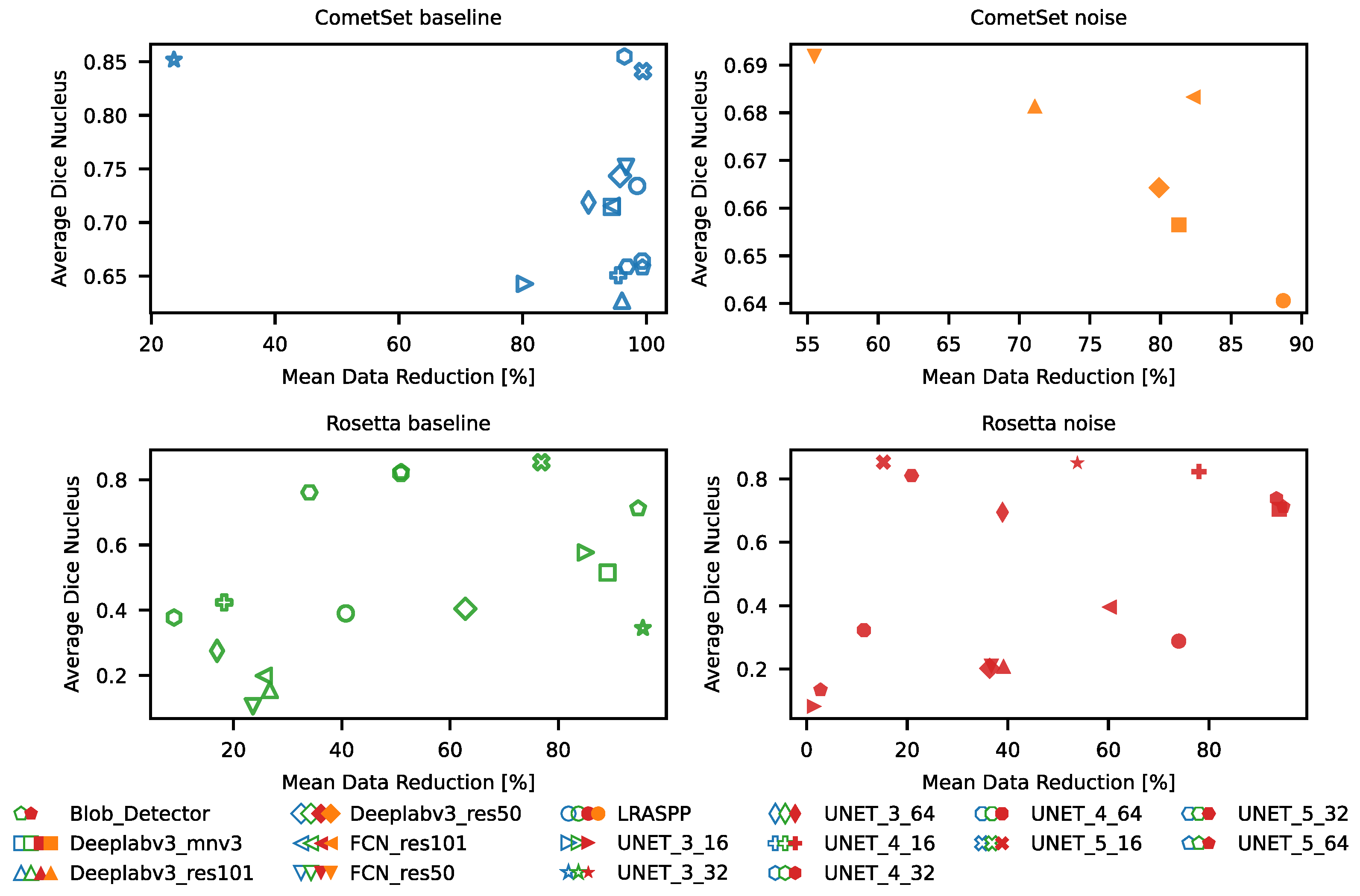
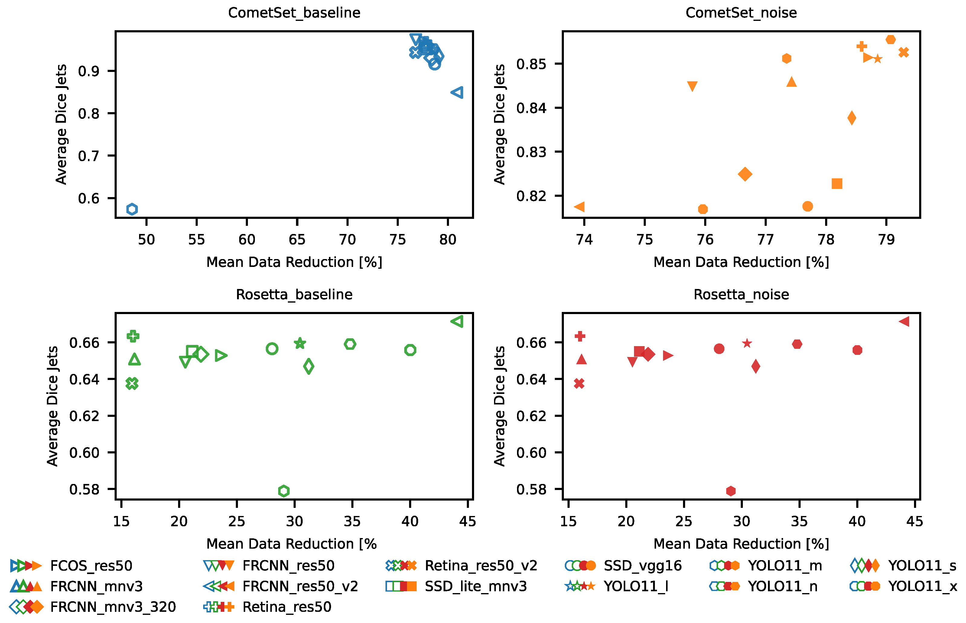
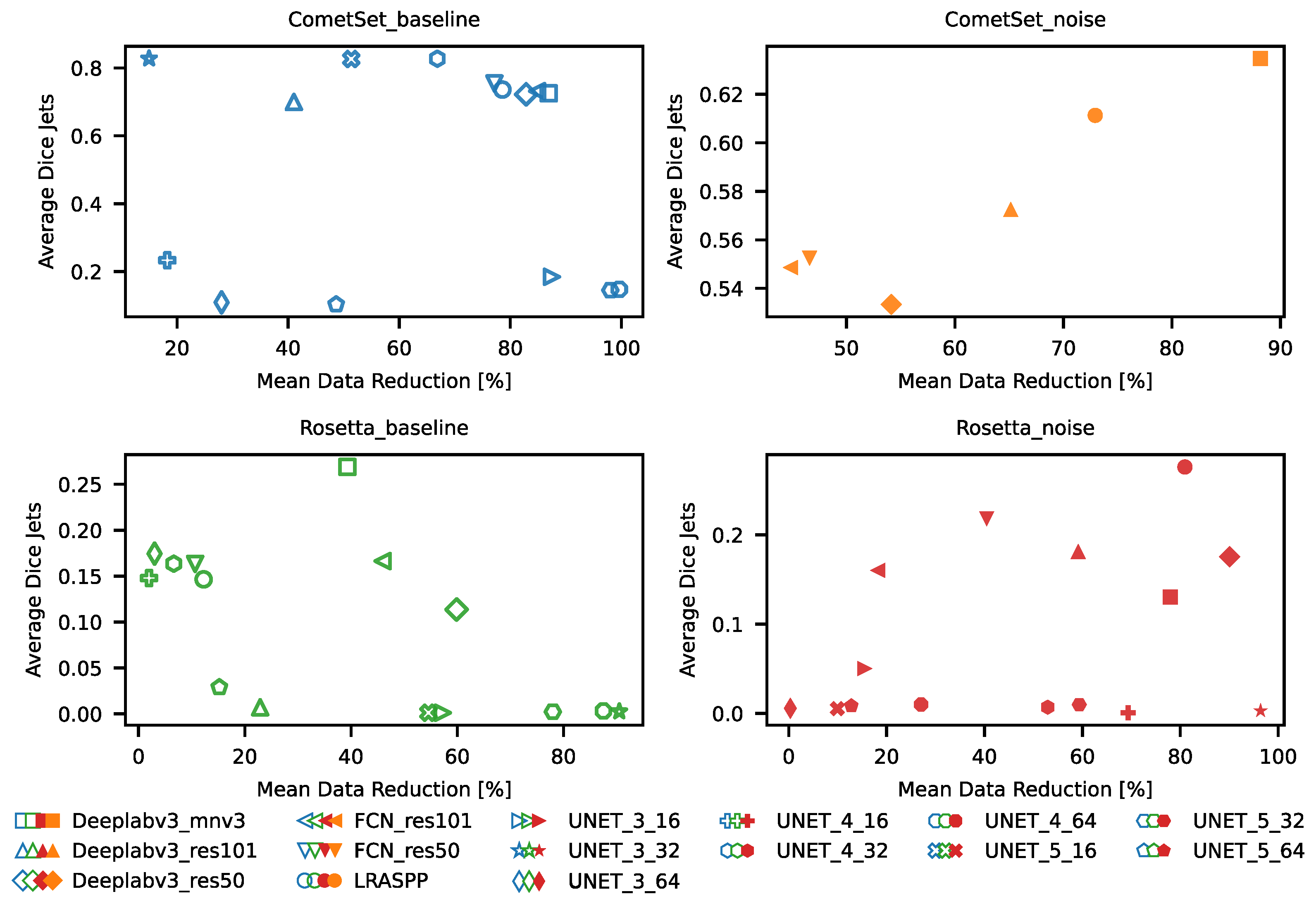
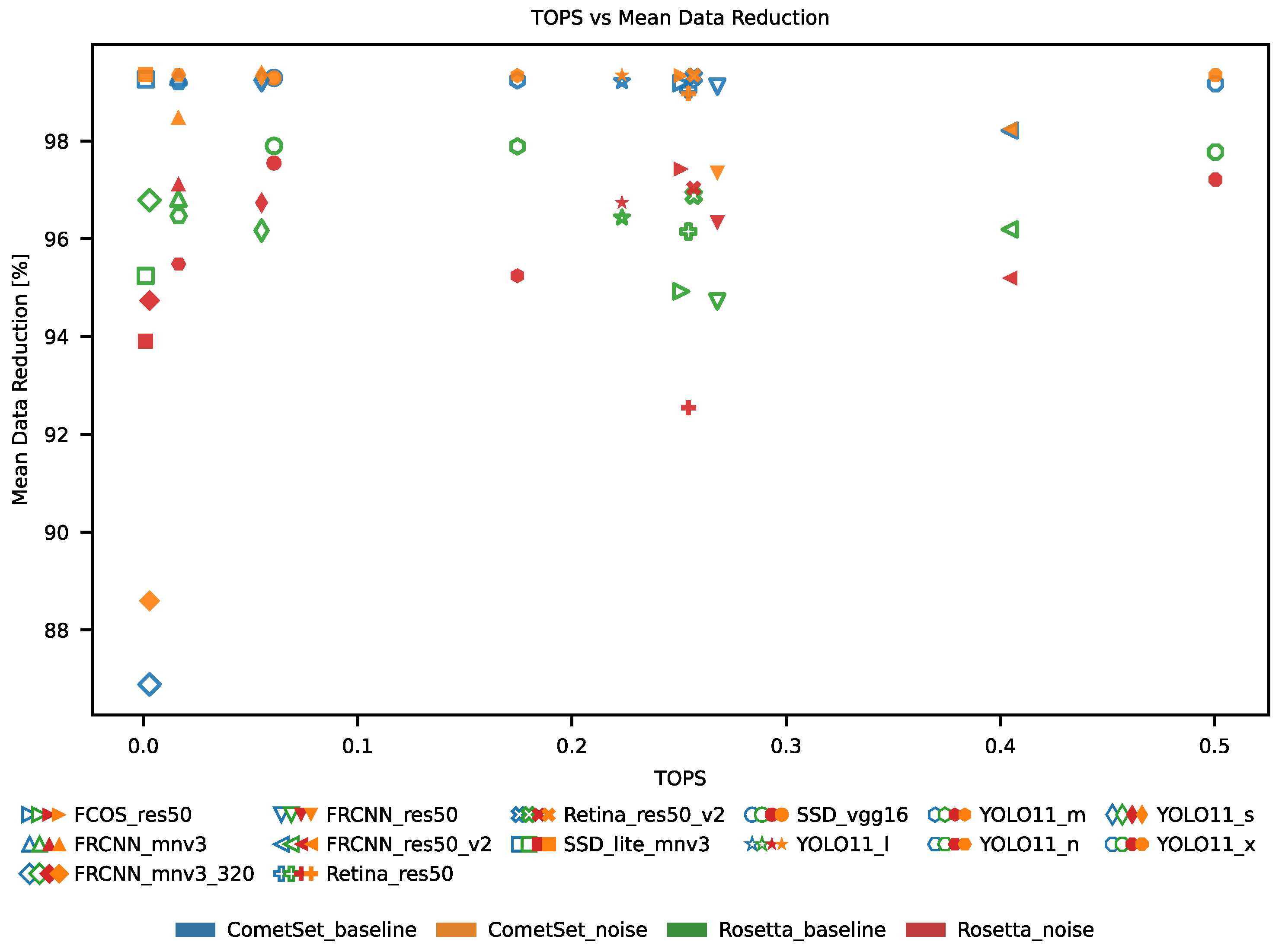
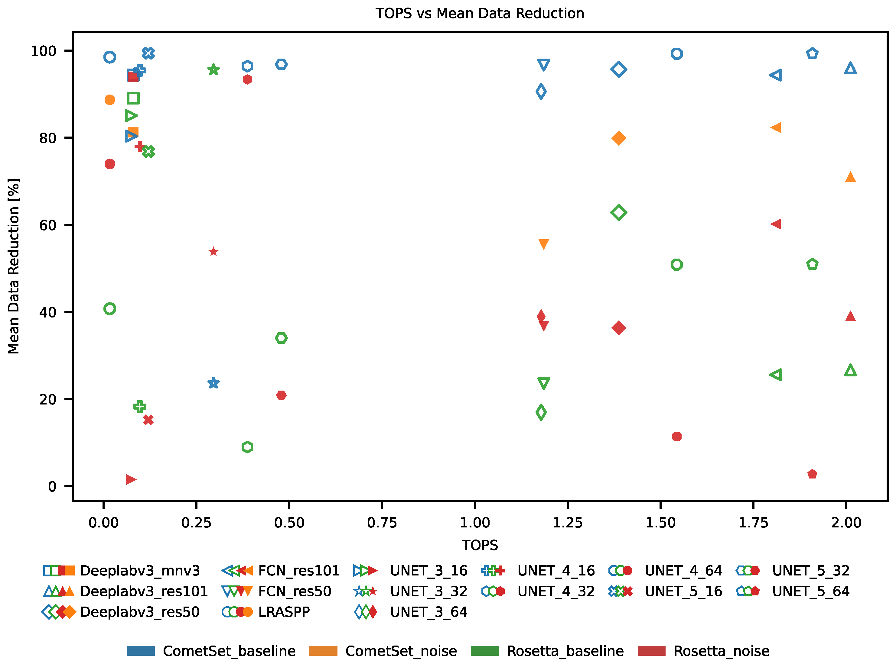
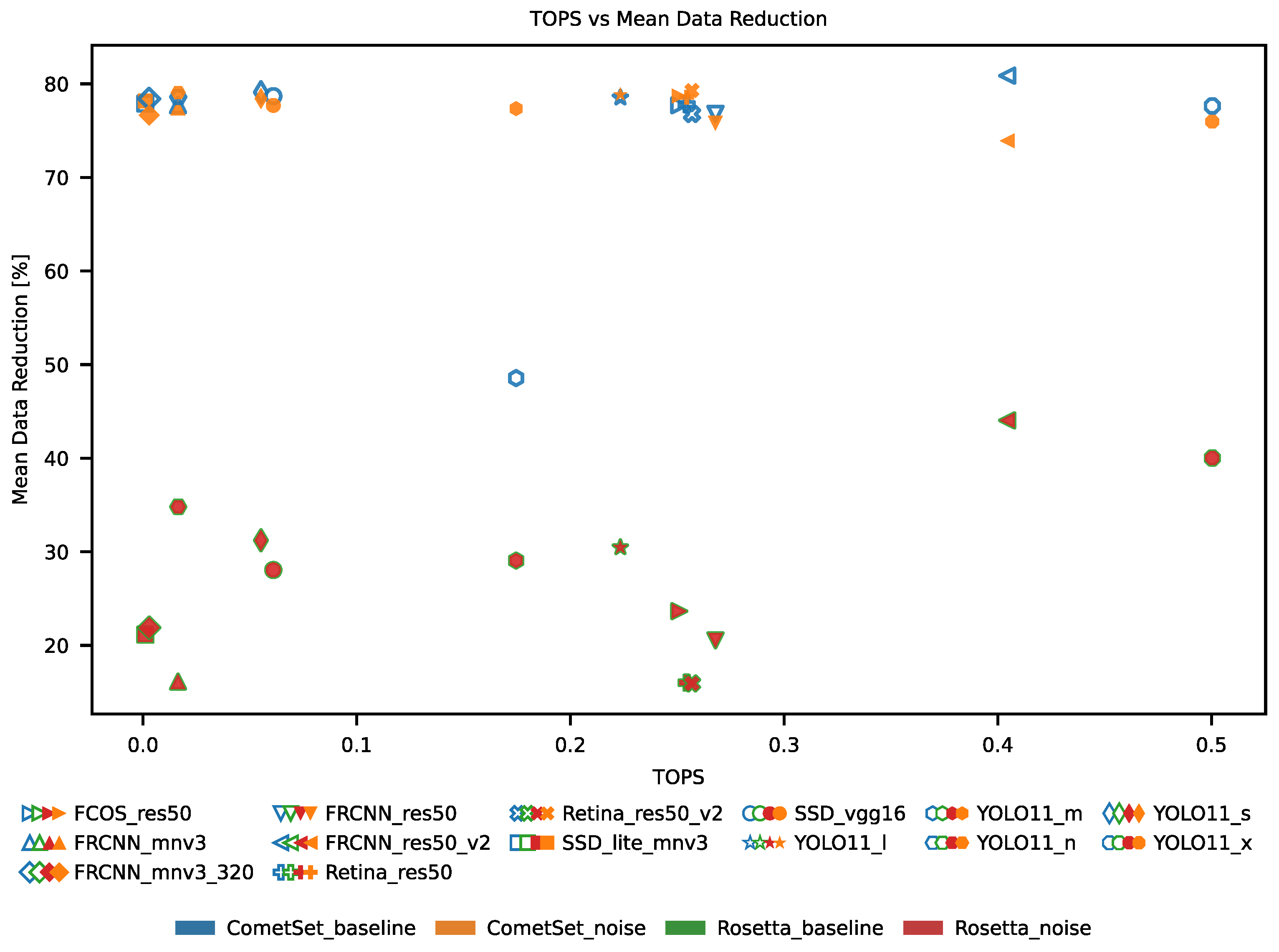
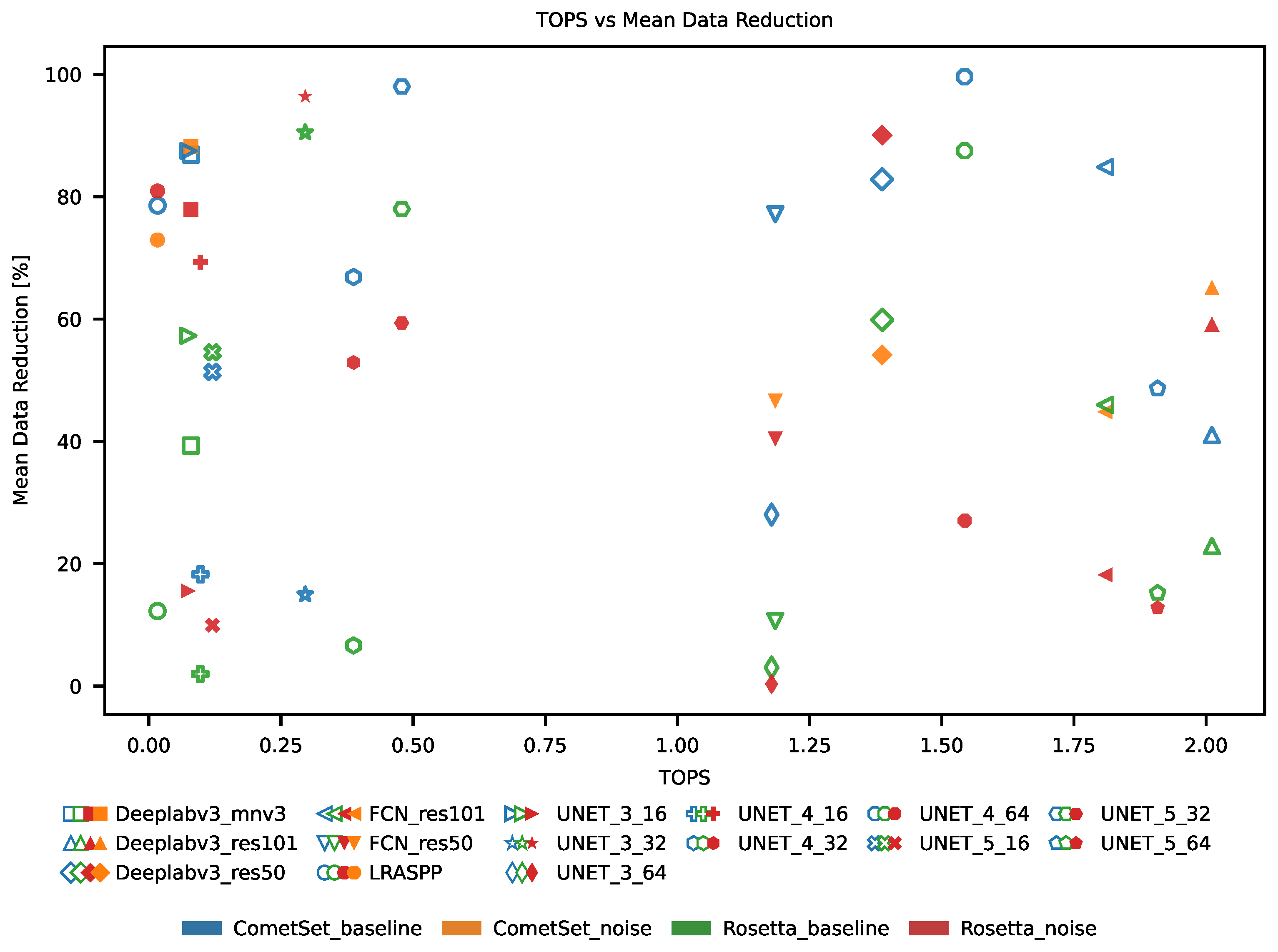
For the main goal of this article, we investigated the achieved data reduction. In Figure 17 and Figure 18, we plot the accuracy of dataset segmentation according to the Dice coefficient vs. the amount of data saved by segmentation for nucleus segmentation, for detection and segmentation, respectively. Figure 19 and Figure 20 show this for jets. The data show that the Dice coefficient and data reduction potential are correlated, so higher segmentation quality generally produces greater gains from data reduction.

3.5. Accuracy vs. Network Complexity

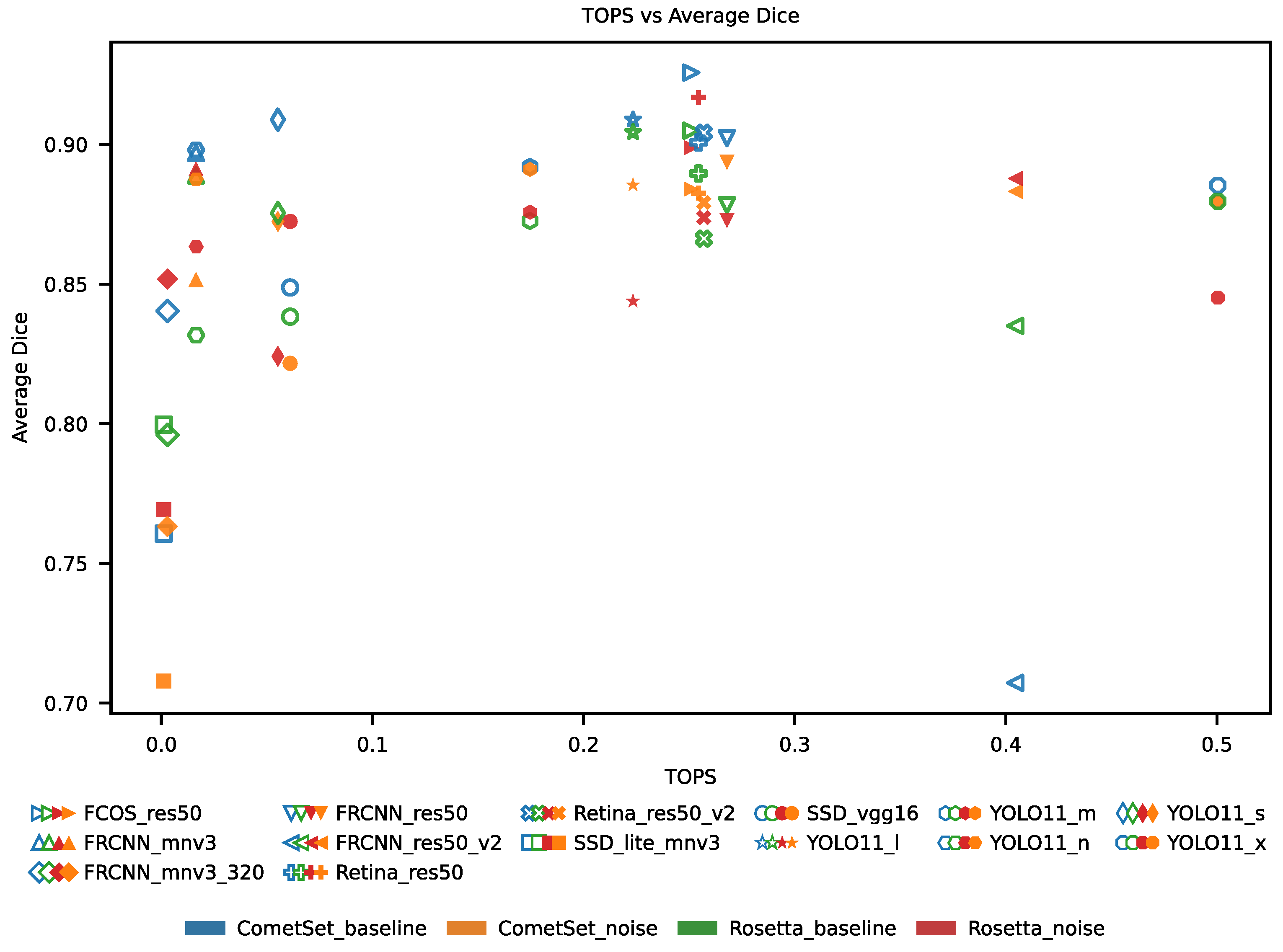
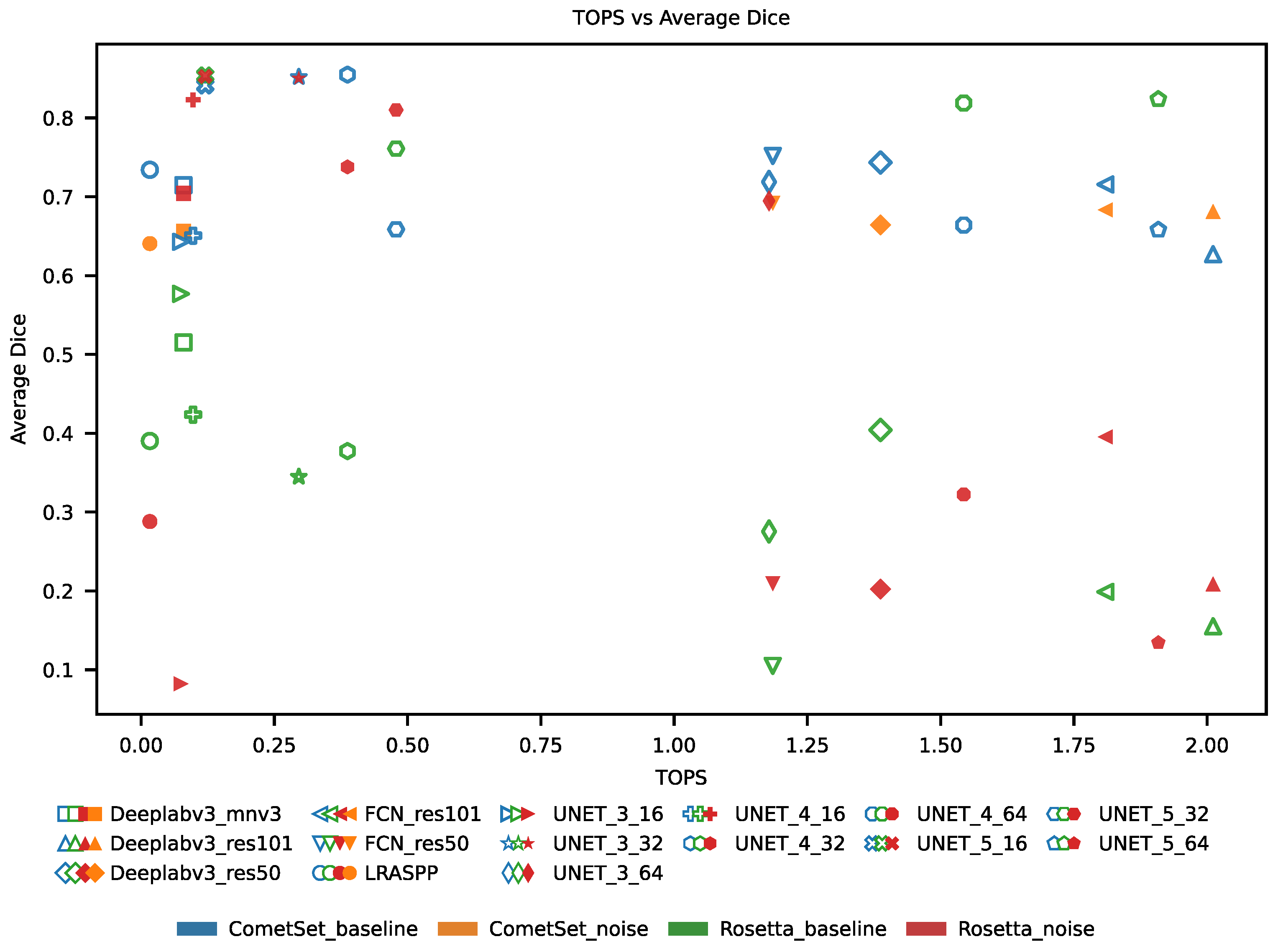
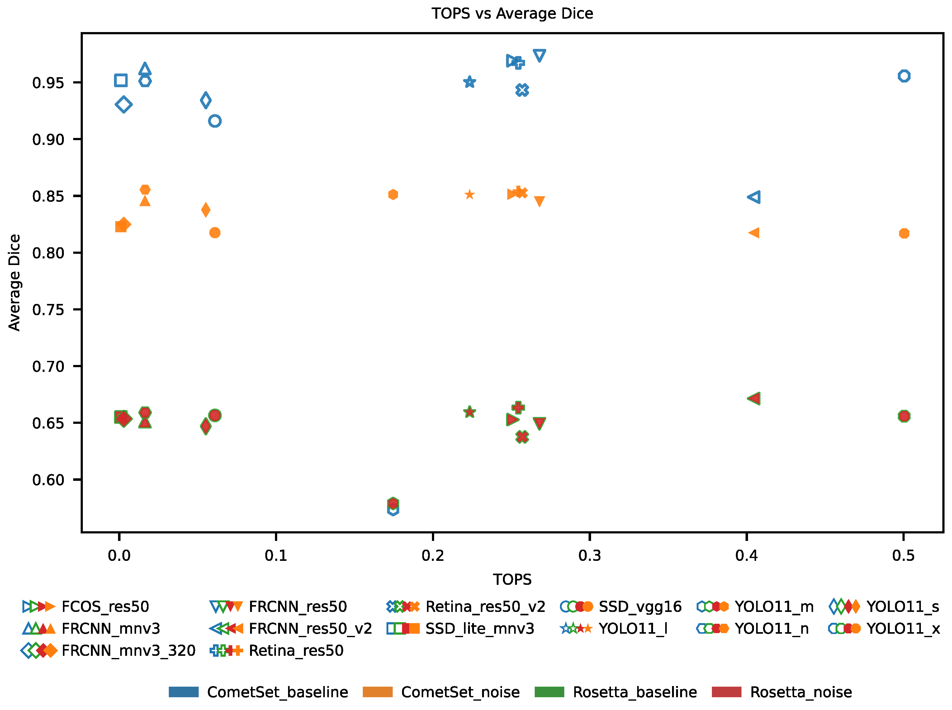
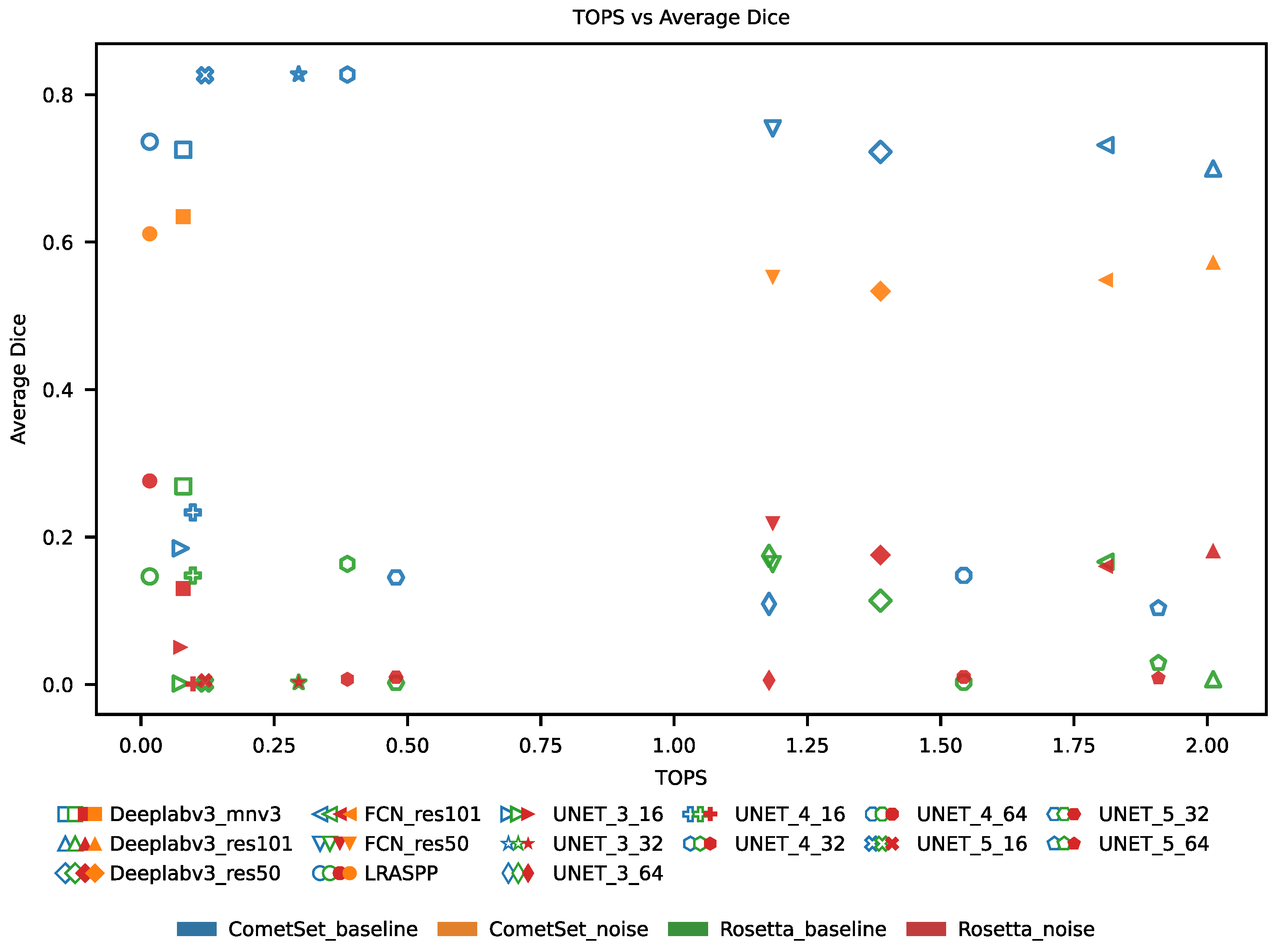
Relationship vs. network accuracy and complexity can be evaluated from Figure 21, Figure 22, Figure 23 and Figure 24 for the case of nucleus detection and segmentation as well as jet detection and segmentation, respectively. It can be seen that network complexity does not significantly affect the results of this analysis.

The only performance drop for detection is seen for the smallest two networks, SSD_lite_mnv3 and FRCNN_mnv3_320. For segmentation, the behaviour is similar; small models tend to perform unexpectedly well.

3.6. Achieved Data Reduction vs. TOPS

Data reduction vs. network complexity shows the same behaviour as accuracy vs. network complexity. This is shown in Figure 25 and Figure 26 for nucleus detection and segmentation, and Figure 27 and Figure 28 for jet detection and segmentation. This demonstrates again that there is no practical benefit to using very large networks and that a useful CNN data reduction system can be built with lower-complexity networks and thus lower-complexity hardware.

4. Discussion

4.1. Data Reduction

Our results show that CNNs can be used to meaningfully reduce onboard data budgets for both nucleus and dust jet segmentation and detection. Specifically the detection networks are stable and achieve promising performance. For dust jets, data reductions of up to 99% are feasible while retaining Dice scores of approximately 0.8 on real data and above 0.8 on synthetic data. This indicates that, with further improvements in generalisation, even higher quality of information retention may be achievable.

The Rosetta Dice score comparison illustrates how models trained on clean synthetic data generalise to real mission data, whereas networks trained with noise augmentation generalise more robustly. Interestingly, not all clean-trained networks perform worse than their noise-trained counterparts on the Rosetta data, suggesting that architecture choice and inductive bias also play significant roles in sim-to-real transfer.

Based on accuracy metrics, several networks demonstrate reliable performance on both synthetic and real datasets, particularly for nucleus detection. In contrast, dust jet detection exhibits notably lower VOC AP@0.5 scores. We suspect that jets are often predicted more correctly by the networks, but the jets in the captured image remain close to or below the noise level, making them difficult to annotate and evaluate reliably, thus making the predictions seem as false positives. This suggests that alternative evaluation metrics may be needed for this task. Another explanation is that the synthetic dust jets in the CometSet dataset are not fully representative of the Rosetta target. Furthermore, class imbalance during training remained a persistent challenge and likely contributed to reduced jet detection performance.

For semantic segmentation, the results show that dust jet segmentation is significantly more challenging than nucleus segmentation. This difficulty is further amplified when translating theoretical pixel-level selection into effective downlink reduction, as efficient compression of irregular segmentation masks remains non-trivial and is beyond the scope of this work.

Importantly, networks trained exclusively on synthetic data remain usable when applied to real Rosetta mission imagery. Although performance metrics on real data are lower overall, this difference is primarily believed to be due to the lack of high-quality ground-truth annotations for the real dataset. Significant improvements in the level of quality of annotation are most likely not possible, because parts of the jets are below the detection limit in the image and thus cannot be reliably annotated. Our current evaluation methodologies heavily penalise this uncertainty when manually annotating real mission data.

When compared to currently deployed approaches such as blob detection and IMPRIO-inspired implementation, the proposed neural network-based methods achieve higher average Dice scores, improved VOC AP@0.5 performance, and greater data reduction. Consequently, these networks offer a more accurate and reliable solution for onboard data selection and enable advanced tasks such as robust dust jet detection.

4.2. Reliability and Failure Modes

Reliability is a key consideration for onboard deployment, particularly for dust jet detection and segmentation, since nucleus detection is generally robust across both synthetic and Rosetta imagery. Under such conditions, models may exhibit partial detections, unstable segmentations, or complete failure cases (i.e., no confident detections or empty/incorrect masks). These failure modes are especially relevant for space missions targeting unknown or dynamically changing scenes, where illumination geometry, background clutter, and sensor noise characteristics may deviate from both the synthetic training distribution and the available real evaluation data.

To obtain a conservative and operationally meaningful estimate of reliability on real imagery, this study reports penalised performance on the Rosetta dataset. Aggregate metrics such as mean Dice and detection precision are computed over the full evaluation set, including samples where the model fails to detect the target or produces invalid outputs. This avoids optimistic bias that would arise from reporting metrics only on successful detections and better reflects end-to-end behaviour in unseen mission conditions, where failure cases directly translate to reduced scientific return or missed opportunities for onboard data prioritisation.

Robustness cannot be guaranteed a priori for all encounter conditions, particularly for dynamically new comets where scene content may deviate from the synthetic training distribution. Practical onboard use should therefore include safeguards for low-confidence predictions and complete failure cases while preserving learned, content-adaptive selection. A simple approach is confidence-based gating with uncertainty padding: when detections or masks are uncertain, the downlink region is conservatively expanded by a margin around the predicted extent, with the margin increasing as confidence decreases. If no reliable prediction is produced for a short interval, the system can temporarily expand around the last confident detection until confidence recovers. Importantly, such safeguards should be mission-generic rather than tuned to a single evaluation dataset, since encounter conditions may differ substantially from both CometSet and Rosetta.

Quantitative reliability assessment on Rosetta imagery is inherently limited by ground-truth uncertainty, particularly for faint dust jets that may be only marginally detectable by human annotators. Since Rosetta annotations are used exclusively for evaluation and not for training, future work could reduce sensitivity to annotation uncertainty through noise-aware or signal-strength-aware evaluation criteria, for example, by incorporating image-specific detectability thresholds or confidence weighting. Manual annotation is only feasible when the signal is visually distinguishable from the background noise, which motivates the use of such detectability thresholds in evaluation.

In addition to annotation uncertainty, a residual domain gap remains between CometSet and Rosetta datasets, and it is most pronounced for dust jet segmentation, where small appearance differences can lead to large pixel-level errors. This gap likely reflects differences in illumination geometry, background complexity, jet morphology, and sensor artefacts that are difficult to fully reproduce synthetically.

4.3. Complexity vs. Performance

The detection results show that it is preferable to use low-complexity networks, as higher-complexity networks provide only diminishing performance gains; thus, larger networks requiring highly complex optimised hardware are not required to make CNN-based data reduction viable. The optimal network processing cost is around 0.02 TOPS, achieved with YOLO11_n.

For segmentation networks, LR-ASPP and DeepLabv3_mnv3 perform comparably to more computationally expensive architectures. LR-ASPP has a cost of 0.02 TOPS, while DeepLabv3_mnv3 has a cost of 0.08 TOPS.

In this context, it is important to note that YOLOv4_tiny has already been used in space applications, although with significant modifications. Two layers were removed, and the model was pruned and quantised. Even so, the base model has a theoretical complexity of approximately 0.04 TOPS, about twice that of YOLO11_n and LR-ASPP. Considering that no other network provides significantly higher Dice scores while remaining computationally efficient, this represents an important finding.

4.4. Hardware Deployability

Hardware deployment remains challenging and is an active topic of research, including by the authors of this work. The most comparable deployment with detailed documentation is presented in [26], which uses YOLOv4-tiny [27]. The need for extensive adaptations to meet size and performance constraints illustrates that the path from network selection and training to actual deployment remains complex. For YOLOv4-tiny, layers were removed, pruning was applied, and quantisation-aware training was performed to enable deployment on the Ubotica CogniSAT-XE2 AI co-processing system.

Considering that both LR-ASPP and YOLO11_n are significantly smaller, fewer optimisation steps may be sufficient to reach deployable configurations. Other missions, such as Intuition-1 by KPLabs [58], report results from competitions and experiments, but detailed deployment strategies are not publicly available. However, due to the use of AMD Zynq Ultrascale+ devices, achievable performance is relatively well understood through existing benchmarks and literature.

Recent preliminary benchmarking results for LR-ASPP are reported in [59], suggesting that even without heavy optimisation, inference speeds comparable to the six frames per second used for OPIC on Comet Interceptor are achievable. This comes at higher power consumption (approximately 6 Watt) compared to the IMPRIO implementation. It should be noted that these results exclude pruning and that the Zynq Ultrascale+ is no longer state-of-the-art. Broader surveys of current accelerator capabilities can be found in [60], with FPGA-specific perspectives in [61]. Most accelerators are not radiation-hardened by design; however, radiation-tolerant variants and component-level radiation testing remain active research areas.

5. Future Research Directions

5.1. Improved Training

During training, especially for segmentation networks, a high risk of early overfitting was observed. This became apparent when analysing loss and Dice curves across epochs. The resulting instability led to varying performance on different test sets, which is particularly visible in the nucleus segmentation results (see Figure 13). Interestingly, some networks performed better on the Rosetta dataset than on the CometSet data, even though Rosetta was not included in the training set. This behaviour requires further investigation and may be related to the Rosetta data being easier to segment than the heavily augmented synthetic dataset.

The challenges of training instability and overfitting could potentially be mitigated through pre-training on more general datasets, followed by fine-tuning on the CometSet. Alternatively, existing pretrained backbone weights could be leveraged more extensively through transfer learning. Given the strong baseline performance of U-Net architectures, this represents a particularly promising direction. Detection networks, however, generally exhibited greater robustness when applied to previously unseen scenarios. Future work will place greater emphasis on pretraining strategies and result stability.

Future work could also reduce the sim-to-real mismatch through improved synthetic realism (e.g., more representative illumination and sensor/noise modelling) and through domain adaptation strategies that leverage unlabelled real images, such as feature-level alignment or self-supervised pretraining followed by synthetic supervision.

5.2. Reducing Computational Complexity

It should be noted that final computational complexity remains to be studied in detail, as no pruning or quantisation was applied to the trained networks. Consequently, the reported TOPS values represent upper bounds, and further reductions are likely possible. Larger networks could be pruned aggressively while maintaining performance, leading to closer convergence in computational cost across networks.

In parallel, alternative optimisation strategies such as custom network architectures are being explored. The results of this work show, for example, through custom U-Net variants, that meaningful performance can be achieved with very small networks, although current reliability remains limited. The LR-ASPP results demonstrate that reliable performance at this scale is feasible. Achieving both high segmentation accuracy and reliability requires further research, particularly in adapting network architectures to the characteristics of the final hardware target.

In addition, trade-offs between sensor-specific pre-processing and network complexity are an interesting avenue. Incorporating more detailed sensor simulations may allow improved network fine-tuning, potentially reducing the need for extensive pre-processing. However, such approaches cannot rely solely on manual, experience-driven optimisation, as they would be difficult to qualify for spaceflight. To address this, reproducibility through automated analysis and optimisation is currently being studied.

5.3. Hardware Deployment

As the overarching goal of this research is to assess whether neural networks on FPGA platforms can improve data selection during automatic fly-bys of unknown targets, a key next step is extensive benchmarking on space-relevant hardware. Hardware deployability is a complex topic and is not explored in depth in this work. A single benchmark on a single device would provide only limited, potentially misleading insight, given the wide range of deployment strategies, optimisation techniques, and hardware platforms.

Nevertheless, it is clear that the best performing networks identified in this study are deployable, as similar architectures have already been flown. The specific deployment strategies and their implications are not yet understood in detail and require more work. The long-term objective is to enable improved onboard data selection using neural networks, as demonstrated in this work, while minimising power consumption and ensuring robust deployment in future missions.

6. Conclusions

In this article, we managed to prove that using CNNs for cometary flyby data reduction is feasible. CNNs are not only more accurate, select data better, and are more reliable on tasks currently performed by algorithms, but it is also possible to perform data reduction for dust jets reliably through object detection CNNs. This was not possible with previous methodologies. Furthermore, training on synthetic data can lead to performance sufficient for real world applications. Lastly, for comet data reduction, the smaller models are sufficiently capable to perform the task. Models of similar complexity have previously been used on space missions [26], demonstrating that comet data reduction is also feasible for future deployment.

References

1. Thompson, D.R.; Anderson, R.C.; Bornstein, B.; Cabrol, N.A.; Chien, S.; Estlin, T.; Fong, T.; Hogan, R.; Lorenz, R.; Gaines, D.; et al. Onboard Science Data Analysis: Implications for Future Missions; Technical Report, Planetary Science Decadal Survey (SBAG Topical White Paper); Jet Propulsion Laboratory, California Institute of Technology: Pasadena, CA, USA, 2008.
2. Ferrari, B.; Cordeau, J.F.; Delorme, M.; Iori, M.; Orosei, R. Satellite Scheduling Problems: A survey of applications in Earth and outer space observation. Comput. Oper. Res. 2025, 173, 106875. [Google Scholar] [CrossRef]
3. Da Poian, V.; Lyness, E.; Danell, R.; Li, X.; Theiling, B.; Trainer, M.; Kaplan, D.; Brinckerhoff, W. Science Autonomy and Space Science: Application to the ExoMars Mission. Front. Astron. Space Sci. 2022, 9, 1–14. [Google Scholar] [CrossRef]
4. Theiling, B.P.; Chou, L.; Da Poian, V.; Battler, M.; Raimalwala, K.; Arevalo, R.J.; Neveu, M.; Ni, Z.; Graham, H.; Elsila, J.; et al. Science Autonomy for Ocean Worlds Astrobiology: A Perspective. Astrobiology 2022, 22, 901–913. [Google Scholar] [CrossRef]
5. Chatar, K.A.A.; Fielding, E.; Sano, K.; Kitamura, K. Data downlink prioritization using image classification on-board a 6U CubeSat. In Proceedings of the Sensors, Systems, and Next-Generation Satellites XXVII; Babu, S.R., Hélière, A., Kimura, T., Eds.; International Society for Optics and Photonics, SPIE: Bellingham, WA, USA, 2023; Volume 12729, p. 127290K. [Google Scholar] [CrossRef]
6. Duggan, A.; Andrade, B.; Afli, H. Advancing Earth observation: A survey on AI-powered image processing in satellites. Eur. J. Remote Sens. 2025, 58, 2567921. [Google Scholar] [CrossRef]
7. Gomez, P.; Meoni, G. Tackling the Satellite Downlink Bottleneck with Federated Onboard Learning of Image Compression. In Proceedings of the 2024 IEEE/CVF Conference on Computer Vision and Pattern Recognition Workshops (CVPRW), Seattle, WA, USA, 17–18 June 2024. [Google Scholar]
8. Justo, J.A.; Ghiţă, A.; Kováč, D.; Garrett, J.L.; Georgescu, M.I.; Gonzalez-Llorente, J.; Ionescu, R.T.; Johansen, T.A. Semantic Segmentation in Satellite Hyperspectral Imagery by Deep Learning. IEEE J. Sel. Top. Appl. Earth Obs. Remote Sens. 2025, 18, 273–293. [Google Scholar] [CrossRef]
9. Giuffrida, G.; Diana, L.; de Gioia, F.; Benelli, G.; Meoni, G.; Donati, M.; Fanucci, L. CloudScout: A Deep Neural Network for On-Board Cloud Detection on Hyperspectral Images. Remote Sens. 2020, 12, 2205. [Google Scholar] [CrossRef]
10. Wang, J.; Feng, Z.; Chen, Z.; George, S.; Bala, M.; Pillai, P.; Yang, S.W.; Satyanarayanan, M. Bandwidth-Efficient Live Video Analytics for Drones Via Edge Computing. In Proceedings of the 2018 IEEE/ACM Symposium on Edge Computing (SEC), Bellevue, WA, USA, 25–27 October 2018; pp. 159–173. [Google Scholar] [CrossRef]
11. Lyu, C.; Lin, S.; Lynch, A.; Zou, Y.; Liarokapis, M. UAV-based deep learning applications for automated inspection of civil infrastructure. Autom. Constr. 2025, 177, 106285. [Google Scholar] [CrossRef]
12. Liu, Y.; Wang, X.; Ning, Z.; Zhou, M.; Guo, L.; Jedari, B. A survey on semantic communications: Technologies, solutions, applications and challenges. Digit. Commun. Netw. 2024, 10, 528–545. [Google Scholar] [CrossRef]
13. Wan, S.; Ding, S.; Chen, C. Edge computing enabled video segmentation for real-time traffic monitoring in internet of vehicles. Pattern Recognit. 2022, 121, 108146. [Google Scholar] [CrossRef]
14. Meoni, G.; Märtens, M.; Derksen, D.; See, K.; Lightheart, T.; Sécher, A.; Martin, A.; Rijlaarsdam, D.; Fanizza, V.; Izzo, D. The OPS-SAT case: A data-centric competition for onboard satellite image classification. Astrodynamics 2024, 8, 507–528. [Google Scholar] [CrossRef]
15. Giuffrida, G.; Fanucci, L.; Meoni, G.; Batič, M.; Buckley, L.; Dunne, A.; van Dijk, C.; Esposito, M.; Hefele, J.; Vercruyssen, N.; et al. The φ-Sat-1 Mission: The First On-Board Deep Neural Network Demonstrator for Satellite Earth Observation. IEEE Trans. Geosci. Remote Sens. 2022, 60, 1–14. [Google Scholar] [CrossRef]
16. Domnich, M.; Sünter, I.; Trofimov, H.; Wold, O.; Harun, F.; Kostiukhin, A.; Järveoja, M.; Veske, M.; Tamm, T.; Voormansik, K.; et al. KappaMask: AI-Based Cloudmask Processor for Sentinel-2. Remote Sens. 2021, 13, 100. [Google Scholar] [CrossRef]
17. Ziaja, M.; Bosowski, P.; Myller, M.; Gajoch, G.; Gumiela, M.; Protich, J.; Borda, K.; Jayaraman, D.; Dividino, R.; Nalepa, J. Benchmarking Deep Learning for On-Board Space Applications. Remote Sens. 2021, 13, 3981. [Google Scholar] [CrossRef]
18. Schuberth, L.; Messina, V.; García Alarcia, R.M.; Sindermann, J.; Bostani Nezhad, K. Leveraging Event-Based Cameras for Enhanced Space Situational Awareness: A Nanosatellite Mission Architecture Study. In Proceedings of the 75th International Astronautical Congress (IAC), Milan, Italy, 14–18 October 2024. Paper code: IAC-24,A6,IP,54,x84856. [Google Scholar]
19. Mateo-García, G.; Veitch-Michaelis, J.; Smith, L.; Oprea, S.V.; Schumann, G.; Gal, Y.; Baydin, A.G.; Backes, D. Towards global flood mapping onboard low cost satellites with machine learning. Sci. Rep. 2021, 11, 7249. [Google Scholar] [CrossRef]
20. Barry, B.; Brick, C.; Connor, F.; Donohoe, D.; Moloney, D.; Richmond, R.; O’Riordan, M.; Toma, V. Always-on Vision Processing Unit for Mobile Applications. IEEE Micro 2015, 35, 56–66. [Google Scholar] [CrossRef]
21. Rodríguez-Bobada, R.; Heredia-Oliver, J.M.; Toledano González, P.T.; Espinosa-Peral, C.; Espinosa-Aranda, J.L.; Hendrix, T.; Perrocheau, A.; Rijlaarsdam, D.; Dunne, A. On-Orbit Validation of an AI-Enabled Cloud Removal and Compression Solution for Earth Observation Satellites. In Proceedings of the 2025 Small Satellite Conference, Salt Lake City, UT, USA, 10–13 August 2025. [Google Scholar] [CrossRef]
22. Rijlaarsdam, D.; Hendrix, T.; González, P.T.T.; Velasco-Mata, A.; Buckley, L.; Miquel, J.P.; Casaled, O.A.; Dunne, A. The Next Era for Earth Observation Spacecraft: An Overview of CogniSAT-6. IEEE J. Sel. Top. Appl. Earth Obs. Remote Sens. 2025, 18, 2450–2463. [Google Scholar] [CrossRef]
23. Grøtte, M.E.; Birkeland, R.; Honoré-Livermore, E.; Bakken, S.; Garrett, J.L.; Prentice, E.F.; Sigernes, F.; Orlandić, M.; Gravdahl, J.T.; Johansen, T.A. Ocean Color Hyperspectral Remote Sensing with High Resolution and Low Latency—The HYPSO-1 CubeSat Mission. IEEE Trans. Geosci. Remote Sens. 2022, 60, 1000619. [Google Scholar] [CrossRef]
24. Bakken, S.; Henriksen, M.B.; Birkeland, R.; Langer, D.D.; Oudijk, A.E.; Berg, S.; Pursley, Y.; Garrett, J.L.; Gran-Jansen, F.; Honoré-Livermore, E.; et al. HYPSO-1 CubeSat: First Images and In-Orbit Characterization. Remote Sens. 2023, 15, 755. [Google Scholar] [CrossRef]
25. Justo, J.A.; Langer, D.D.; Berg, S.; Nieke, J.; Ionescu, R.T.; Kjeldsberg, P.G.; Johansen, T.A. Hyperspectral Image Segmentation for Optimal Satellite Operations: In-Orbit Deployment of 1D-CNN. Remote Sens. 2025, 17, 642. [Google Scholar] [CrossRef]
26. Day, P.; Crane, J.; Cronk, P.; Jimenez, C.; Johnson, B.; Koeberle, R.; Millard, D.; Werner, Z. Experimental Results from On-orbit Edge-deployed AI Detection of Resident Space Objects Using Computer Vision. In Advanced Maui Optical and Space Surveillance Technologies Conference (AMOS 2024), Proceedings of the 25th Advanced Maui Optical and Space Surveillance Technologies Conference (AMOS), Maui, HI, USA, 17–20 September 2024; Maui Economic Development Board, Inc.: Kihei, HI, USA, 2024. [Google Scholar]
27. Bochkovskiy, A.; Wang, C.Y.; Liao, H.Y.M. YOLOv4: Optimal Speed and Accuracy of Object Detection. arXiv 2020, arXiv:2004.10934. [Google Scholar] [CrossRef]
28. Snodgrass, C.; Jones, G.H. The European Space Agency’s Comet Interceptor lies in wait. Nat. Commun. 2019, 10, 5418. [Google Scholar] [CrossRef] [PubMed]
29. Jones, G.H.; Snodgrass, C.; Tubiana, C.; Küppers, M.; Kawakita, H.; Lara, L.M.; Agarwal, J.; André, N.; Attree, N.; Auster, U.; et al. The Comet Interceptor Mission. Space Sci. Rev. 2024, 220, 9. [Google Scholar] [CrossRef]
30. Snodgrass, C.; Epifani, E.M.; Tubiana, C.; Sánchez, J.P.; Biver, N.; Inno, L.; Knight, M.M.; Lacerda, P.; Keyser, J.D.; Donaldson, A.; et al. Considerations on the process of target selection for the Comet Interceptor mission. Icarus 2026, 447, 116887. [Google Scholar] [CrossRef]
31. Pajusalu, M.; Kivastik, J.; Iakubivskyi, I.; Slavinskis, A. Developing Autonomous Image Capturing Systems for Maximum Science Yield for High Fly-by Velocity Small Solar System Body Exploration. In Proceedings of the 71st International Astronautical Congress (IAC 2020), Virtual Event, 12–14 October 2020. IAC CyberSpace Edition 2020; IAF Space Exploration Symposium, Session A3.4B: Small Bodies Missions and Technologies (Part 2). [Google Scholar]
32. Dengel, R.; Pajusalu, M. A Synthetic Image Data Generation Pipeline for Spacecraft Fly-by Scenarios. In Proceedings of the 2023 European Data Handling & Data Processing Conference (EDHPC), Juan-Les-Pins, France, 2–6 October 2023; pp. 1–8. [Google Scholar] [CrossRef]
33. Blender Foundation. Blender—A 3D Creation Suite [Computer Software]. Version 3.x Series Used in This Work. 2025. Available online: https://www.blender.org (accessed on 26 January 2026).
34. Dengel, R.; Pajusalu, M. CometSet. Zenodo. 2025. Available online: https://zenodo.org/records/16635768 (accessed on 26 January 2026).
35. Glassmeier, K.H.; Boehnhardt, H.; Kührt, E.; Richter, I. The Rosetta Mission: Flying Towards the Origin of the Solar System. Space Sci. Rev. 2007, 128, 1–21. [Google Scholar] [CrossRef]
36. Taylor, M.G.G.T. The Rosetta mission orbiter science overview: The comet phase. Philos. Trans. R. Soc. A 2017, 375, 20160262. [Google Scholar] [CrossRef]
37. Geiger, B.; Barthelemy, M. Rosetta NAVCAM Comet Escort Phase Data. Dataset RO-C-NAVCAM-3-ESCORT-V1.0. 2017. Available online: https://archives.esac.esa.int/psa (accessed on 26 January 2026).
38. Keller, H.U.; Barbieri, C.; Koschny, D.; Rickman, H.; Rodrigo, R.; Wenzel, K.-P.; Sierks, H.; A’hearn, M.F.; Angrilli, F.; Angulo, M.; et al. OSIRIS—The Scientific Camera System Onboard Rosetta. Space Sci. Rev. 2007, 128, 433–506. [Google Scholar] [CrossRef]
39. Sierks, H.; OSIRIS Team. Rosetta-OSIRIS Comet Escort Phase Data. Dataset RO-C-OSIRIS-3-ESCORT-V1.0. 2019. Available online: https://archives.esac.esa.int/psa (accessed on 26 January 2026).
40. Bitlake Technologies. IMPRIO IP Core: Image Prioritization for the OPIC Instrument in ESA’s Comet Interceptor Mission. 2023. Available online: https://bitlaketech.com/imprio-ip-core-image-prioritization-for-the-opic-instrument-in-esas-comet-interceptor-mission/ (accessed on 29 December 2025).
41. Šate, J.; Smirnova, A.; Briede, E.; Zapāns, V. IMPRIO IP Core: FPGA-Based Image Prioritization for Autonomous Operations in ESA’s Comet Interceptor Mission. Presentation, SpacE FPGA Users Workshop (SEFUW), ESA/ESTEC. 2025. Available online: https://indico.esa.int/event/531/contributions/10600/attachments/6585/11685/Bitlake_SEFUW_2025_27032025.pdf (accessed on 26 January 2026).
42. OpenCV Team. OpenCV: Open Source Computer Vision Library. 2024. Available online: https://opencv.org (accessed on 26 January 2026).
43. Otsu, N. A Threshold Selection Method from Gray-Level Histograms. IEEE Trans. Syst. Man Cybern. 1979, 9, 62–66. [Google Scholar] [CrossRef]
44. Long, J.; Shelhamer, E.; Darrell, T. Fully Convolutional Networks for Semantic Segmentation. In Proceedings of the 2015 IEEE Conference on Computer Vision and Pattern Recognition (CVPR), Boston, MA, USA, 7–12 June 2015; pp. 3431–3440. [Google Scholar] [CrossRef]
45. Howard, A.; Sandler, M.; Chu, G.; Chen, L.C.; Chen, B.; Tan, M.; Wang, W.; Zhu, Y.; Pang, R.; Vasudevan, V.; et al. Searching for MobileNetV3. In Proceedings of the 2019 IEEE/CVF International Conference on Computer Vision (ICCV), Seoul, Republic of Korea, 27 October–2 November 2019; pp. 1314–1324. [Google Scholar] [CrossRef]
46. Chen, L.C.; Papandreou, G.; Schroff, F.; Adam, H. Rethinking Atrous Convolution for Semantic Image Segmentation. arXiv 2017, arXiv:1706.05587. [Google Scholar] [CrossRef]
47. Ronneberger, O.; Fischer, P.; Brox, T. U-Net: Convolutional Networks for Biomedical Image Segmentation. In Lecture Notes in Computer Science, Proceedings of the Medical Image Computing and Computer-Assisted Intervention (MICCAI), Munich, Germany, 5–9 October 2015; Springer: Berlin/Heidelberg, Germany, 2015; pp. 234–241. [Google Scholar] [CrossRef]
48. Ren, S.; He, K.; Girshick, R.; Sun, J. Faster R-CNN: Towards Real-Time Object Detection with Region Proposal Networks. In Proceedings of the Advances in Neural Information Processing Systems (NeurIPS), Montreal, QC, Canada, 7–12 December 2015. [Google Scholar]
49. Lin, T.Y.; Goyal, P.; Girshick, R.; He, K.; Dollár, P. Focal Loss for Dense Object Detection. In Proceedings of the 2017 IEEE International Conference on Computer Vision (ICCV), Venice, Italy, 22–29 October 2017; pp. 2980–2988. [Google Scholar] [CrossRef]
50. Tian, Z.; Shen, C.; Chen, H.; He, T. FCOS: Fully Convolutional One-Stage Object Detection. In Proceedings of the 2019 IEEE/CVF International Conference on Computer Vision (ICCV), Seoul, Republic of Korea, 27 October–2 November 2019; pp. 9627–9636. [Google Scholar] [CrossRef]
51. Liu, W.; Anguelov, D.; Erhan, D.; Szegedy, C.; Reed, S.; Fu, C.Y.; Berg, A.C. SSD: Single Shot MultiBox Detector. In Lecture Notes in Computer Science, Proceedings of the Computer Vision—ECCV 2016, Amsterdam, The Netherlands, 11–14 October 2016; Springer: Berlin/Heidelberg, Germany, 2016; pp. 21–37. [Google Scholar] [CrossRef]
52. Ultralytics. YOLOv11: Real-Time Object Detection. Technical Documentation and Pretrained Models. 2025. Available online: https://github.com/ultralytics/ultralytics (accessed on 26 January 2026).
53. Lin, T.Y.; Dollár, P.; Girshick, R.; He, K.; Hariharan, B.; Belongie, S. Feature pyramid networks for object detection. In Proceedings of the 2017 IEEE Conference on Computer Vision and Pattern Recognition (CVPR), Honolulu, HI, USA, 21–26 July 2017; pp. 2117–2125. [Google Scholar]
54. Dice, L.R. Measures of the Amount of Ecologic Association Between Species. Ecology 1945, 26, 297–302. [Google Scholar] [CrossRef]
55. Everingham, M.; Van Gool, L.; Williams, C.K.I.; Winn, J.; Zisserman, A. The PASCAL Visual Object Classes (VOC) Challenge. Int. J. Comput. Vis. 2010, 88, 303–338. [Google Scholar] [CrossRef]
56. Lin, T.Y.; Maire, M.; Belongie, S.; Bourdev, L.; Girshick, R.; Hays, J.; Perona, P.; Ramanan, D.; Dollár, P.; Zitnick, C.L. Microsoft COCO: Common Objects in Context. In Lecture Notes in Computer Science, Proceedings of the European Conference on Computer Vision (ECCV), Zurich, Switzerland, 5–12 September 2014; Springer: Berlin/Heidelberg, Germany, 2014; pp. 740–755. [Google Scholar] [CrossRef]
57. Everingham, M.; Eslami, S.M.A.; Van Gool, L.; Williams, C.K.I.; Winn, J.; Zisserman, A. The PASCAL Visual Object Classes Challenge: A Retrospective. Int. J. Comput. Vis. 2015, 111, 98–136. [Google Scholar] [CrossRef]
58. Wijata, A.M.; Foulon, M.F.; Bobichon, Y.; Vitulli, R.; Celesti, M.; Camarero, R.; Di Cosimo, G.; Gascon, F.; Longépé, N.; Nieke, J.; et al. Taking Artificial Intelligence Into Space Through Objective Selection of Hyperspectral Earth Observation Applications: To bring the “brain” close to the “eyes” of satellite missions. IEEE Geosci. Remote Sens. Mag. 2023, 11, 10–39. [Google Scholar] [CrossRef]
59. Dengel, R.; Pajusalu, M.; Laufer, R. Utilising SpaceChipExplorer to Benchmark Data Reduction Performance on FPGAs in Space. In Proceedings of the 76th International Astronautical Congress (IAC), International Astronautical Federation, Sydney, Australia, 29 September–3 October 2025. [Google Scholar]
60. Mystkowska, G.; Monopoli, M.; Nannipieri, P.; Zulberti, L.; Codinachs, D.M.; Fanucci, L. Hardware Platforms Enabling Edge AI for Space Applications: A Critical Review. IEEE Access 2025, 13, 143939–143956. [Google Scholar] [CrossRef]
61. Antunes, P.; Podobas, A. FPGA-Based Neural Network Accelerators for Space Applications: A Survey. arXiv 2025, arXiv:cs.AR/2504.16173. [Google Scholar] [CrossRef]
Figure 1. (Left) CometSet example including all object rendered. (Right) CometSet example including all object masks.
Aerospace 13 00128 g001
Figure 2. Some sample images from the Rosetta datasets utilised for testing CNNs.
Aerospace 13 00128 g002
Figure 3. (Left) Synthetic image from Comet Dataset. (Center) Noise augmentation applied on the image. (Right) Comparable image from Rosetta Archives.
Aerospace 13 00128 g003
Figure 4. Example output from the IMPRIO-inspired algorithm (Left). Image from Rosetta Dataset (Right). Detection from IMPRIO-inspired algorithm and subsequent cropped region.
Aerospace 13 00128 g004
Figure 5. Example output from the OpenCV-based simple blob detection as baseline comparison method (Left). Input image to algorithm (Middle). Binary mask of detected blob (Right). Bounding box/segmentation output and corresponding cropping.
Aerospace 13 00128 g005
Figure 6. Sample of CNN predictions on Comet Dataset and Rosetta Dataset.
Aerospace 13 00128 g006
Figure 7. Qualitative comparison of detection outputs from the YOLO11_n model on a noisy image (left) from the Rosetta dataset. The baseline model (middle) produces an overly extended dust jet detection, while the model trained on noise-augmented synthetic data (right) yields a more spatially constrained and stable prediction under identical conditions.
Aerospace 13 00128 g007
Figure 8. Bar plot with dice performance for all detection networks evaluated on both qualitatively annotated Rosetta data and CometSet Test split, containing results for both jets and nucleus. Clean and noisy bars are trained on clean and noisy data, respectively, but the evaluation data are inherently noisy.
Aerospace 13 00128 g008
Figure 9. Bar plot with dice performance for all segmentation networks evaluated on both qualitatively annotated Rosetta data and CometSet Test split, containing results for both jets and nucleus. Clean and noisy bars are trained on clean and noisy data, respectively, but the evaluation data are inherently noisy.
Aerospace 13 00128 g009
Figure 10. Bar plot with dice performance for all detection networks evaluated on both qualitatively annotated Rosetta data and CometSet Test split, containing only results for the detection of the comet nucleus. Clean and noisy bars are trained on clean and noisy data, respectively, but the evaluation data are inherently noisy.
Aerospace 13 00128 g010
Figure 11. Bar plot with dice performance for all segmentation networks evaluated on both qualitatively annotated Rosetta data and CometSet Test split, containing only results for the segmentation of the comet nucleus. Clean and noisy bars are trained on clean and noisy data, respectively, but the evaluation data are inherently noisy.
Aerospace 13 00128 g011
Figure 12. Bar plot with dice performance for all detection networks evaluated on both qualitatively annotated Rosetta data and CometSet Test split, containing only results for the detection of jets. Clean and noisy bars are trained on clean and noisy data, respectively, but the evaluation data are inherently noisy.
Aerospace 13 00128 g012
Figure 13. Bar plot with dice performance for all segmentation networks evaluated on both qualitatively annotated Rosetta data and CometSet Test split, containing only results for the segmentation of jets. Clean and noisy bars are trained on clean and noisy data, respectively, but the evaluation data are inherently noisy.
Aerospace 13 00128 g013
Figure 14. Bar plot with VOC AP@0.5 for all detection networks evaluated on both qualitatively annotated Rosetta data and CometSet Test split, containing results for both jets and nucleus. Clean and noisy bars are trained on clean and noisy data, respectively, but the evaluation data are inherently noisy.
Aerospace 13 00128 g014
Figure 15. Bar plot with VOC AP@0.5 for all segmentation networks evaluated on both qualitatively annotated Rosetta data and CometSet Test split, containing results for nucleus class. Clean and noisy bars are trained on clean and noisy data, respectively, but the evaluation data are inherently noisy.
Aerospace 13 00128 g015
Figure 16. Bar plot with VOC AP@0.5 for all detection networks evaluated on both qualitatively annotated Rosetta data and CometSet Test split, containing only results for the detection of the comet jets. Clean and noisy bars are trained on clean and noisy data, respectively, but the evaluation data are inherently noisy.
Aerospace 13 00128 g016
Figure 17. Scatter plots for the datasets used for nucleus detection, showing the average Dice coefficient vs. mean data reduction for detection networks.
Aerospace 13 00128 g017
Figure 18. Scatter plots for the datasets used for nucleus segmentation, showing the average Dice coefficient vs. mean data reduction for detection networks.
Aerospace 13 00128 g018
Figure 19. Scatter plots for the datasets used for jet detection, showing the average Dice coefficient vs. mean data reduction for detection networks.
Aerospace 13 00128 g019
Figure 20. Scatter plots for the datasets used for jet segmentation, showing the average Dice coefficient vs. mean data reduction for detection networks.
Aerospace 13 00128 g020
Figure 21. Scatter plots showing the relation between Dice coefficient and TOPS for each detection network for the datasets used for nucleus detection.
Aerospace 13 00128 g021
Figure 22. Scatter plots showing the relation between Dice coefficient and TOPS for each segmentation network for the datasets used for nucleus segmentation.
Aerospace 13 00128 g022
Figure 23. Scatter plots showing the relation between Dice coefficient and TOPS for each detection network for the datasets used for jet detection.
Aerospace 13 00128 g023
Figure 24. Scatter plots showing the relation between Dice coefficient and TOPS for each segmentation network for the datasets used for jet segmentation.
Aerospace 13 00128 g024
Figure 25. Scatter plots showing the relation between mean data reduction and TOPS for each detection network for the datasets used for nucleus detection.
Aerospace 13 00128 g025
Figure 26. Scatter plots showing the relation between mean data reduction and TOPS for each detection network for the datasets used for nucleus segmentation.
Aerospace 13 00128 g026
Figure 27. Scatter plots showing the relation between mean data reduction and TOPS for each detection network for the datasets used for jet detection.
Aerospace 13 00128 g027
Figure 28. Scatter plots showing the relation between mean data reduction and TOPS for each detection network for the datasets used for jet segmentation.
Aerospace 13 00128 g028