Three-Dimensional Prescribed-Time Convergent Cooperative Integrated Guidance and Control for Multiple STT Vehicles with Terminal Angle Constraints and Actuator Faults

Abstract

A cooperative integrated guidance and control (CIGC) scheme is proposed for multiple- skid-to-turn (STT) vehicles subject to terminal angle constraints and actuator faults. Following the principle of “single-vehicle design first, cooperative extension afterward”, the proposed method integrates prescribed-time sliding mode control, a prescribed-time disturbance observer, dynamic surface control, and nonlinear filtering into a unified IGC framework, ensuring prescribed-time stability of the single-vehicle closed-loop system while enhancing robustness against model uncertainties and actuator faults. Furthermore, a graph-theoretic adaptive cooperative guidance law is developed to generate the desired acceleration command, and a prescribed-time velocity controller is designed to track the command. As a result, all vehicles achieve prescribed-time consensus of the remaining flight time and coordinated arrival at the terminal point at the prescribed time. The stability of the closed-loop system is rigorously established through Lyapunov analysis. Numerical simulation results demonstrate that compared to existing methods, the proposed scheme achieves faster convergence and stronger robustness.

1. Introduction

Flight vehicles are generally classified into axisymmetric and planar-symmetric vehicles. Axisymmetric vehicles typically employ skid-to-turn (STT) control, maintaining a near-zero roll angle and regulating the flight direction through pitch and sideslip motions. Planar-symmetric vehicles generally adopt bank-to-turn (BTT) control, maintaining a near-zero sideslip angle and regulating the flight direction through roll and pitch motions. This study focuses on the design of a guidance and control system for axisymmetric vehicles. Conventional flight vehicles adopt separate designs for guidance and control systems. However, this separation neglects the coupling between the two systems, preventing full exploitation of their performance [1]. Therefore, an integrated guidance and control (IGC) design approach is adopted to improve the guidance and control accuracy of flight vehicles.

Most existing IGC methods assume small attack and sideslip angles. Under this assumption, the coupling among the roll, pitch, and yaw channels is neglected, and the system is decomposed into three independent channels [2]. Owing to the strict-feedback structure, backstepping control and sliding mode control have been widely adopted in IGC design [3]. To avoid the differential explosion caused by repeated differentiation of virtual control inputs, dynamic surface control (DSC) with filters has been introduced [4]. Guo et al. [5] proposed full-state sliding mode control to directly generate actuator commands without virtual control inputs. More recently, both linear and nonlinear model predictive control have been applied to IGC design [6]. Zhou et al. [7] employed Koopman-operator-based LMPC to address aerodynamic nonlinearities, while Cui et al. [8] developed an optimized NMPC to reduce the computational burden of nonlinear systems. However, these methods either require considerable computational effort or exhibit limited robustness against model uncertainties and external disturbances. More importantly, these methods are generally established under the assumption of decoupled channels, whereas three-dimensional vehicle dynamics inherently exhibit strong cross-channel coupling.

By contrast, three-channel coupled IGC explicitly accounts for the coupling among the roll, pitch, and yaw channels, thereby improving guidance and control performance [9]. For three-dimensional STT vehicles, Wang et al. [10] developed an IGC scheme with actuator saturation constraints based on a high-order nonlinear model, dynamic surface control, and the Nussbaum function. Luo et al. [11] combined a fractional-order extended state observer with backstepping-based active disturbance rejection control to compensate for lumped disturbances and measurement noise. Wang et al. [12] incorporated state constraints and an event-triggered mechanism into the IGC design to improve control efficiency, while Wei et al. [13] established a high-precision BLOS-based nonlinear model and proposed a prescribed-time IGC scheme under field-of-view constraints. Although these studies have achieved significant progress in nonlinear modelling, robust control, and state-constrained guidance, the desired terminal angle constraint has not been adequately addressed.

For high-precision terminal guidance tasks, terminal angle constraints play an important role in ensuring that the vehicle approaches the terminal point along a prescribed direction [14]. Existing terminal angle control methods can generally be categorized into finite-time [15], fixed-time [16], and prescribed-time approaches [17,18]. Wang et al. [19] proposed a finite-time IGC scheme based on time-varying sliding mode control. Li et al. [20] and Zhang et al. [21] further developed fixed-time IGC schemes using dynamic surface control and non-singular terminal sliding mode control. The latter scheme ensured global fixed-time convergence through a fixed-time reaching law. Compared to finite-time and fixed-time convergence, prescribed-time convergence enables the convergence time to be explicitly assigned a priori. Cui et al. [22] applied prescribed-time control to a partially integrated IGC scheme in the two-dimensional longitudinal plane, while Cui et al. [23] extended prescribed-time IGC to BTT vehicles. Nevertheless, existing prescribed-time IGC studies are mainly limited to BTT vehicles or two-dimensional scenarios, and only the LOS elevation constraint is considered. To the best of the authors’ knowledge, prescribed-time IGC for three-dimensional STT vehicles with simultaneous LOS elevation and azimuth angle constraints has not yet been reported.

In practical systems, actuators exhibit hysteresis characteristics [24], and under near-space combat environments, they may also suffer from additive and multiplicative faults [25]. To address actuator fault problems, [26] designed an adaptive controller based on radial basis function neural networks and the Actor–Critic framework, enabling normal operation in the presence of actuator faults. In Wang et al. [27], actuator faults and external disturbances were treated as lumped disturbances and compensated using a disturbance observer. In Chen et al. [28], both hysteresis and fault characteristics were simultaneously considered. An IGC scheme was developed using dynamic surface control and adaptive laws to ensure the stability and reliability of the closed-loop system. However, in that study, actuator faults were considered prior to first-order lag dynamics; this treatment is inconsistent with actual physical characteristics. Moreover, fault-tolerant control was realized under the assumption of known fault coefficients, without considering unknown fault coefficients.

Based on the above analysis of the IGC design model regarding three-dimensional coupling and channel-decoupled schemes, convergence control subject to terminal angle constraints, and actuator faults, this work adopts a three-dimensional coupled IGC framework to capture the inter-channel coupling effects. To realize the convergence of system states as well as the line-of-sight elevation and azimuth angles, the prescribed-time convergence theory is employed to achieve a faster convergence rate. Existing studies that simultaneously consider actuator faults and first-order lag usually treat the fault factor as a known parameter for direct compensation. In contrast, a disturbance observer is constructed in this paper to estimate and compensate for such unknown disturbances. The research gaps compared to existing studies are summarized in

Table 1. Comparison of research gaps for IGC design.

Method	Dim	Terminal Angle	Additional Processing	Controller
Guo et al. [5]	2-D decoupled	-	Range-limited	Fixed-time SMC
Wang et al. [12]	3-D decoupled	Elevation + Azimuth	Event-triggered	DSC
Wei et al. [13]	3-D decoupled	Elevation + Azimuth	Field-of-view angle constraints	Fixed-time SMC
Wang et al. [19]	3-D coupled	Elevation + Azimuth	Input Saturation	Finite-Time SMC
Cui et al. [23]	3-D coupled	Elevation	Spiral maneuvering deceleration	Prescribed-time SMC
Chen et al. [28]	3-D coupled	-	Actuator fault + First-lag (known fault coefficients)	DSC
Proposed method	3-D coupled	Elevation + Azimuth	Actuator fault + First-lag (Unknown fault coefficients)	Prescribed-time SMC

.

Furthermore, the increasing complexity of three-dimensional guidance tasks has imposed higher requirements on the coordination of multiple flight vehicles [29]. Consequently, cooperative guidance and control strategies for multiple flight vehicles subject to terminal angle constraints have attracted increasing attention. Existing cooperative integrated guidance and control (CIGC) methods can be broadly classified into three categories. The first category specifies a nominal relative distance between each vehicle and the target, and each vehicle tracks this nominal value to accomplish the cooperative guidance task. Wang et al. [30] proposed a two-dimensional cooperative guidance strategy based on the nominal remaining flight distance, while Li et al. [31] extended it to three-dimensional engagements with LOS azimuth angle constraints. However, this method assumes a constant vehicle velocity, which is inconsistent with practical flight conditions. The second category adopts a leader–follower architecture, in which follower vehicles track the leader through local information exchange [32]. Cui et al. [33] further developed a prescribed-time CIGC scheme for BTT–STT hybrid vehicles. However, the failure of the leader may significantly degrade the cooperative performance and even destabilize the entire formation. The third category is based on graph theory, where cooperative coordination is achieved through distributed information exchange among neighbouring vehicles [34,35]. Zhang et al. [21] combined a graph-theoretic cooperative guidance law with a fixed-time IGC scheme to accomplish the cooperative guidance task. However, existing studies directly use the desired velocity generated by the cooperative guidance law as the actual vehicle velocity input. This neglects the modelling of the propulsion system and its controller, which is inconsistent with practical engineering realities.

Synthesizing the above existing CIGC approaches, this work develops a graph-theoretic cooperative guidance law integrated with a thrust model, a velocity controller and the aforementioned IGC scheme. The proposed strategy fulfils the cooperative mission while accounting for terminal angle constraints and actuator faults. A comparison of the research frameworks is given in

Table 2. Comparison of research gaps for CIGC design.

Method	Cooperative Mechanism	Terminal Angle	Actuator Fault	Velocity Control	System Stability
Wang et al. [30]	Nominal relative distance	-	-	Constant velocity	Asymptotic Stability
Li et al. [31]	Nominal relative distance	Azimuth	-	Constant velocity	Asymptotic Stability
Cui et al. [33]	Leader–follower	Azimuth	-	Aerodynamic drag deceleration	Prescribed-time Stability
Zhang et al. [21]	Graph theory	Elevation + Azimuth	-	Desired velocity command	Fixed-time Stability
Proposed method	Graph theory	Elevation + Azimuth	Actuator fault + First-order lag	Thrust + velocity control	Prescribed-time Stability

.

Although existing control systems have achieved relatively fast convergence, it is still of research value to further improve the convergence speed. Meanwhile, studies on CIGC that simultaneously consider cooperation, terminal angle constraints, and actuator faults are still limited. A prescribed-time IGC scheme that simultaneously handles LOS elevation and azimuth angles is developed for STT vehicles. The scheme adopts thrust-driven velocity control and accommodates unknown actuator fault coefficients. By further combining the graph-theory-based cooperative guidance law, the proposed IGC framework is extended to a CIGC architecture for multi-vehicle coordinated missions. The main contributions are summarized as follows:

• A prescribed-time convergent IGC scheme is developed for vehicles subject to terminal angle constraints and actuator faults. Based on prescribed-time convergence theory, all system states converge to their desired values within a prescribed time independent of the initial conditions. Unlike fixed-time control, the convergence time is independent of multiple design parameters [19,20,21]. It should be noted that existing prescribed-time IGC schemes are mainly developed for BTT vehicles and only consider LOS azimuth angle constraints, whereas their application to STT vehicles with simultaneous LOS elevation and azimuth angle constraints has not yet been investigated [23]. Moreover, the IGC scheme proposed in this paper achieves a faster convergence rate than existing fixed-time and prescribed-time IGC schemes.
• A prescribed-time disturbance observer is developed to compensate for disturbances and actuator faults. Compared to existing observers [24,31], it guarantees disturbance estimation within a prescribed time independent of initial conditions, while providing an explicitly specified convergence time compared to adaptive laws [26,27,28]. Furthermore, actuator faults are modelled as unknown parameters and compensated via the disturbance observer, making the proposed method more practical than [28], which assumes known fault factors.
• A leaderless cooperative guidance law is designed based on graph theory and integrated with the proposed IGC scheme. The remaining flight times of all vehicles reach consensus within a fixed time, enabling simultaneous target interception at the prescribed arrival time. Unlike conventional guidance methods [34,36,37], the proposed CIGC scheme explicitly incorporates vehicle dynamics, actuator characteristics, and thrust-based velocity control. In contrast to [21], where the desired velocity is directly treated as the actual vehicle velocity, the proposed method explicitly considers thrust and velocity dynamics.

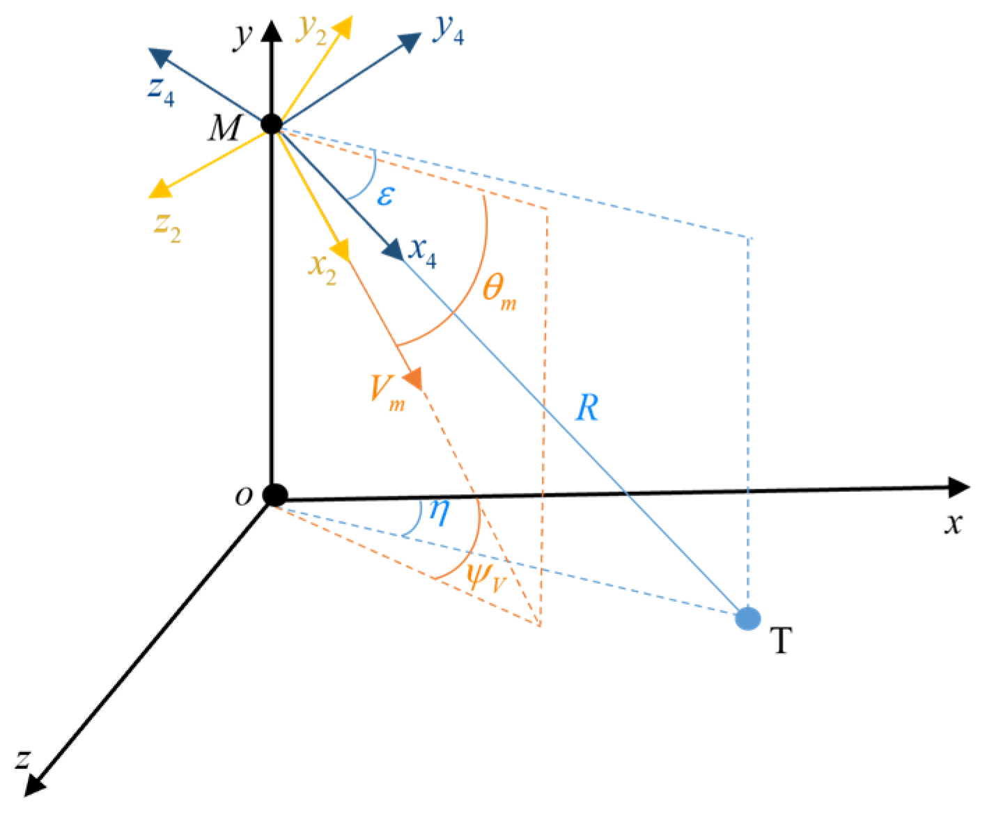
The remainder of this paper is organized as follows: Section 2 establishes the six-degree-of-freedom STT vehicle model and the three-dimensional integrated guidance and control design model considering actuator faults. Section 3 develops a globally prescribed-time convergent CIGC algorithm based on the Lyapunov method. Section 4 presents numerical simulations to verify the effectiveness of the proposed algorithm. Section 5 concludes the paper.

Due to the large number of symbols involved in the paper, the notation and symbol definitions are provided in Nomenclature.

2. Problem Formulation

This section consists of the six-degree-of-freedom axisymmetric vehicle, the relative motion between the vehicle and the target, the first-order actuator fault model and the IGC design model.

2.1. Six-Degree-of-Freedom Axisymmetric Vehicle Model

The six-degree-of-freedom kinematics and dynamics model is as follows:

$$\left\{\begin{array}{l}\dot{x}=V_m\cos {\theta }_m\cos {\psi }_V\\ \dot{y}=V_m\sin {\theta }_m\\ \dot{z}=-V_m\cos {\theta }_m\sin {\psi }_V\\ {\dot{V}}_m={\displaystyle \frac{P\cos \alpha \cos \beta -X-mg\sin {\theta }_m}{m}}\\ {\dot{\theta }}_m={\displaystyle \frac{P(\sin \alpha \cos {\gamma }_v+\cos \alpha \sin \beta \sin {\gamma }_v)+Y\cos {\gamma }_V-Z\sin {\gamma }_V-mg\cos {\theta }_m}{m{V}_m}}\\ {\dot{\psi }}_V=-{\displaystyle \frac{P(\sin \alpha \sin {\gamma }_v-\cos \alpha \sin \beta \cos {\gamma }_v)+Y\sin {\gamma }_V+Z\cos {\gamma }_V}{m{V}_m\cos {\theta }_m}}\\ {\dot{\omega }}_x={\displaystyle \frac{J_y-J_z}{J_x}}{\omega }_z{\omega }_y+{\displaystyle \frac{1}{J_x}}{M}_x+{\Delta }_{\omega x}\\ {\dot{\omega }}_y={\displaystyle \frac{J_z-J_x}{J_y}}{\omega }_x{\omega }_z+{\displaystyle \frac{1}{J_y}}{M}_y+{\Delta }_{\omega y}\\ {\dot{\omega }}_z={\displaystyle \frac{J_x-J_y}{J_z}}{\omega }_x{\omega }_y+{\displaystyle \frac{1}{J_z}}{M}_z+{\Delta }_{\omega z}\\ \dot{\alpha }=-{\omega }_x\cos \alpha \tan \beta +{\omega }_y\sin \alpha \tan \beta +{\omega }_z-{\displaystyle \frac{P\sin \alpha +Y-mg\cos {\theta }_m\cos {\gamma }_V}{m{V}_m\cos \beta }}+{\Delta }_{\alpha }\\ \dot{\beta }={\omega }_x\sin \alpha +{\omega }_y\cos \alpha -{\displaystyle \frac{P\cos \alpha \sin \beta -Z-mg\cos {\theta }_m\sin {\gamma }_V}{m{V}_m}}+{\Delta }_{\beta }\\ {\dot{\gamma }}_V={\omega }_x\cos \alpha \sec \beta -{\omega }_y\sin \alpha \sec \beta +{\displaystyle \frac{1}{m{V}_m}}(P_t+Y(\tan \theta \sin {\gamma }_V+\tan \beta )\\ +Z\tan {\theta }_m\cos {\gamma }_V-mg\tan \beta \cos {\theta }_m\cos {\gamma }_V)+{\Delta }_{\gamma V}\\ P_t=P(\sin \alpha \tan \beta \sin {\gamma }_V-\cos \alpha \sin \beta \tan {\theta }_m\cos {\gamma }_V+\tan \beta \sin \alpha )\end{array}\right.$$

(1)

where $x$, $y$, and $z$ represent the position in the inertial coordinate system, and $V_m$ represents velocity; ${\theta }_m$ and ${\psi }_V$ represent the flight path angle and heading angle, respectively; ${\omega }_x$, ${\omega }_y$, and ${\omega }_Z$ represent roll, yaw, and pitch rates; $J_x$, $J_y$, and $J_z$ are roll, yaw, and pitch moments of inertia; $M_x$, $M_y$, and $M_z$ are roll, yaw, pitch moments; $\alpha$, $\beta$, and ${\gamma }_V$ represent airflow angles, including angle of attack, sideslip, and velocity roll angles, respectively; $m$ represents the mass of the vehicle; $g$ represents the local gravitational acceleration; $X$, $Y$, and $Z$ represent drag, lift, side force, respectively; ${\Delta }_{\omega x}$, ${\Delta }_{\omega y}$, ${\Delta }_{\omega z}$, ${\Delta }_{\alpha }$, ${\Delta }_{\beta }$, ${\Delta }_{\gamma V}$ are modelling errors and external disturbances; $P$ denotes the engine thrust, and $P_t$ represents a function of $P$.

The aerodynamic forces and moments of the axisymmetric vehicle are approximated by the following fitted expressions:

$$\left\{\begin{array}{l}X=qS(c_{x0}+c_x^{\alpha }\left|\alpha \right|+c_x^{\beta }\left|\beta \right|+c_x^{\alpha \beta }\left|\alpha \beta \right|+c_x^{\delta x}\left|{\delta }_x\right|+c_x^{\delta y}\left|{\delta }_y\right|+c_x^{\delta z}\left|{\delta }_z\right|)\\ Y=qS(c_y^{\alpha }\alpha +c_y^{\beta }\beta )\\ Z=qS(c_z^{\alpha }\alpha +c_z^{\beta }\beta )\\ M_x=qSL(m_{x0}+m_x^{\alpha }\alpha +m_x^{\beta }\beta +m_x^{\delta x}{\delta }_x+m_x^{\delta y}{\delta }_y)\\ M_y=qSL(m_{y0}+m_y^{\beta }\beta +m_y^{\delta y}{\delta }_y+m_y^{\delta x}{\delta }_x)\\ M_z=qSL(m_{z0}+m_z^{\alpha }\alpha +m_z^{\delta z}{\delta }_z)\end{array}\right.$$

(2)

where $q$ represents dynamic pressure; $S$ represents reference area; $L$ represents reference length; ${\delta }_x$, ${\delta }_y$, and ${\delta }_z$ represent roll, yaw, and pitch surface fin deflections, respectively; $c_{x0}$, $c_x^{\alpha }$, $c_x^{\beta }$, $c_x^{\alpha \beta }$, $c_x^{\beta }$, $c_x^{\delta x}$, $c_x^{\delta y}$, and $c_x^{\delta z}$ represent zero-lift drag coefficient, and the partial derivatives of the drag coefficient with respect to $\alpha$, $\beta$, ${\delta }_x$, ${\delta }_y$, ${\delta }_z$, respectively. Similarly, the coefficients $c_y^{\alpha }$, $c_y^{\beta }$, $c_z^{\alpha }$, $c_z^{\beta }$, $m_{x0}$, $m_{y0}$, $m_{z0}$, $m_x^{\alpha }$, $m_x^{\beta }$, $m_x^{\delta y}$, $m_x^{\delta x}$, $m_y^{\beta }$, $m_y^{\delta y}$, $m_y^{\delta z}$, $m_z^{\alpha }$, $m_z^{\delta z}$ represent various coefficients related to aerodynamic forces and moments. As the vehicle is axisymmetric, $m_{x0}$, $m_{y0}$, and $m_{z0}$ are zero.

2.2. Three-Dimensional Relative Motion Between the Vehicle and Target

The three-dimensional relative geometry between the vehicle and the target is illustrated in Figure 1. During the terminal guidance phase, the Earth is assumed to be flat, and the vehicle is considered to move in the inertial coordinate system $Oxyz$. The trajectory coordinate system of the vehicle is denoted as $M{x}_2{y}_2{z}_2$. The $M$ is located at the vehicle’s centre of mass, and the axis $M{x}_2$ is aligned with the vehicle velocity vector $V_m$. The axis $M{y}_2$ lies in the vertical plane and is perpendicular to $M{x}_2$, pointing upward. The axis $M{z}_2$ is perpendicular to $M{y}_2$ and $M{x}_2$ which is determined by the right-hand rule. The ${\theta }_m$ is the flight angle between the vehicle velocity vector and the plane $Oxz$, and ${\psi }_V$ is the heading angle between the axis $Ox$ and the projection of the vehicle velocity vector onto the plane $Oxz$. The line-of-sight (LOS) coordinate system of the vehicle is denoted as $M{x}_4{y}_4{z}_4$. The axis $M{x}_4$ coincides with the LOS direction. The axis $M{y}_4$ lies in the vertical plane and is perpendicular to $M{x}_4$, pointing upward. The axis $M{z}_4$ is perpendicular to $M{y}_4$ and $M{x}_4$, which is determined by the right-hand rule. The $\epsilon$ is the LOS elevation angle between $M{x}_4$ and the plane $Oxyz$, and $\eta$ is the LOS azimuth angle between the projection of onto the plane $Oxz$ and the axis $Ox$.

In the LOS coordinate system, the relative motion equations between the vehicle and the target can be expressed as

$$\left[\begin{array}{l}{a}_{tR}\\ a_{t\epsilon }\\ a_{t\eta }\end{array}\right]-\left[\begin{array}{l}{a}_{mR}\\ a_{m\epsilon }\\ a_{m\eta }\end{array}\right]=\left[\begin{array}{c}\ddot{R}-R{\dot{\epsilon }}^2-R{\dot{\eta }}^2{\cos }^2\epsilon \\ R\ddot{\epsilon }+2\dot{R}\dot{\epsilon }+R{\dot{\eta }}^2\sin \epsilon \cos \epsilon \\ -2\dot{R}\dot{\eta }\cos \epsilon -R\ddot{\eta }\cos \epsilon +2R\dot{\epsilon }\dot{\eta }\sin \epsilon \end{array}\right]$$

(3)

where ${\mathit{a}}_{m4}={[a_{mR},a_{m\epsilon },a_{m\eta }]}^T$ and ${\mathit{a}}_{t4}={[a_{tR},a_{t\epsilon },a_{t\eta }]}^T$ which represent the projections of the acceleration of the vehicle and the target in the LOS coordinate system, respectively. According to [31], by combining the transformation of the vehicle acceleration from the trajectory coordinate system to the LOS coordinate system with (3), one can obtain

$$\left[\begin{array}{l}\ddot{\epsilon }\\ \ddot{\eta }\end{array}\right]={\mathit{F}}_1+{\mathit{G}}_1\left[\begin{array}{c}\alpha \\ \beta \end{array}\right]+{\mathit{d}}_1$$

(4)

with

$${\mathit{F}}_1=\left[\begin{array}{c}{\displaystyle \frac{-2\dot{R}\dot{\epsilon }-R{\dot{\eta }}^2\sin \epsilon \cos \epsilon }{R}}\\ {\displaystyle \frac{-2\dot{R}\dot{\eta }\cos \epsilon +2R\dot{\epsilon }\dot{\eta }\sin \epsilon }{R\cos \epsilon }}\end{array}\right]+{\overline{\mathit{B}}}_R{\overline{\mathit{B}}}_1\left[\begin{array}{c}-g\cos {\theta }_m\\ 0\end{array}\right]+{\overline{\mathit{B}}}_R\left[\begin{array}{c}{\dot{V}}_m(\cos \epsilon \sin {\theta }_m-\cos {\theta }_m\sin \epsilon \cos (\eta -{\psi }_V))\\ {\dot{V}}_m\cos {\theta }_m\sin (\eta -{\psi }_V)\end{array}\right]$$

$${\mathit{G}}_1={\displaystyle \frac{qS}{m}}{\overline{\mathit{B}}}_R{\overline{\mathit{B}}}_1{\overline{\mathit{B}}}_{\gamma V}{\overline{\mathit{B}}}_c,{\mathit{d}}_1=\left[\begin{array}{c}{\displaystyle \frac{a_{t\epsilon }}{R}}\\ -{\displaystyle \frac{a_{t\eta }}{R\cos \epsilon }}\end{array}\right]$$

(5)

where

$$\begin{array}{c}{\overline{\mathit{B}}}_{\gamma V}=\left[\begin{array}{cc}\cos {\gamma }_V& -\sin {\gamma }_V\\ \sin {\gamma }_V& \cos {\gamma }_V\end{array}\right]{\overline{\mathit{B}}}_C=\left[\begin{array}{cc}{c}_y^{\alpha }& c_y^{\beta }\\ c_z^{\alpha }& c_z^{\beta }\end{array}\right]{\overline{\mathit{B}}}_R=\left[\begin{array}{cc}-{\displaystyle \frac{1}{R}}& 0\\ 0& {\displaystyle \frac{1}{R\cos \epsilon }}\end{array}\right]\\ {\overline{\mathit{B}}}_1=\left[\begin{array}{cc}\cos \epsilon \sin {\theta }_m+\sin {\theta }_m\sin \epsilon \cos (\eta -{\psi }_V)& \sin \epsilon \sin (\eta -{\psi }_V)\\ -\sin {\theta }_m\sin (\eta -{\psi }_V)& \cos (\eta -{\psi }_V)\end{array}\right]\end{array}$$

2.3. First-Order Actuator Fault Model

The first-order faulty actuator model not only accounts for the dynamic hysteresis in the actuator response, but also simultaneously describes the additive and multiplicative faults of the actuator.

The first-order actuator model with hysteresis is given as follows:

$$\left[\begin{array}{l}{\dot{\delta }}_{xc}\\ {\dot{\delta }}_{yc}\\ {\dot{\delta }}_{zc}\end{array}\right]=-{\displaystyle \frac{1}{\xi }}\left[\begin{array}{l}{\delta }_{xc}\\ {\delta }_{yc}\\ {\delta }_{zc}\end{array}\right]+{\displaystyle \frac{1}{\xi }}\left[\begin{array}{l}{\delta }_{xd}\\ {\delta }_{yd}\\ {\delta }_{zd}\end{array}\right]$$

(6)

where ${\delta }_{xd}$, ${\delta }_{yd}$, and ${\delta }_{zd}$ denotes the ideal control input, ${\delta }_{xc}$, ${\delta }_{yc}$, and ${\delta }_{zc}$ represents the output of the first-order lag of the actuator. $\xi$ represents the gain of the first-order lag.

The actuator model considering both additive and multiplicative faults is expressed as follows:

$$\left[\begin{array}{l}{\delta }_x\\ {\delta }_y\\ {\delta }_z\end{array}\right]=\left[\begin{array}{c}{h}_x{\delta }_{xc}\\ h_y{\delta }_{yc}\\ h_z{\delta }_{zc}\end{array}\right]+\left[\begin{array}{c}{\upsilon }_x\\ {\upsilon }_y\\ {\upsilon }_z\end{array}\right]$$

(7)

where ${\delta }_x$, ${\delta }_y$, and ${\delta }_z$ denotes the actual control output obtained by applying actuator faults to the first-order lag output of the actuator. $h_x$, $h_y$, and $h_z$ are availability health indicator gains, whose values are bounded within $[0,1]$, where $h_{x,y,z}=1$ represents a healthy actuator and $h_{x,y,z}=0$ represents complete loss of actuator effectiveness. ${\upsilon }_x$, ${\upsilon }_y$, and ${\upsilon }_z$ are bias fault signals, whose magnitudes are bounded by the maximum actuator deflection ${\delta }_{\max }$.

Taking the derivative of (7) and combining it with (6) and (7) yields

$$\left[\begin{array}{l}{\dot{\delta }}_x\\ {\dot{\delta }}_y\\ {\dot{\delta }}_z\end{array}\right]=-{\displaystyle \frac{1}{\xi }}\left[\begin{array}{l}{\delta }_x\\ {\delta }_y\\ {\delta }_z\end{array}\right]+{\displaystyle \frac{1}{\xi }}\left[\begin{array}{l}{h}_x{\delta }_{xd}+{\upsilon }_x\\ h_y{\delta }_{yd}+{\upsilon }_y\\ h_z{\delta }_{zd}+{\upsilon }_z\end{array}\right]+\left[\begin{array}{l}{\displaystyle \frac{{\dot{h}}_x}{h_x}}({\delta }_x-{\upsilon }_x)+{\dot{\upsilon }}_x\\ {\displaystyle \frac{{\dot{h}}_y}{h_y}}({\delta }_y-{\upsilon }_y)+{\dot{\upsilon }}_y\\ {\displaystyle \frac{{\dot{h}}_z}{h_z}}({\delta }_z-{\upsilon }_z)+{\dot{\upsilon }}_z\end{array}\right]$$

(8)

There exists ${\delta }_{\max }$ and ${\dot{\delta }}_{\max }$ such that the desired control input $\left|{\delta }_{xd,yd,zd}\right|\le {\delta }_{\max }$, the actual actuator input $\left|{\delta }_{x,y,z}\right|\le {\delta }_{\max }$, and the deflection rate satisfies the upper bound $\left|{\dot{\delta }}_{x,y,z}\right|\le {\dot{\delta }}_{\max }$.

2.4. Three-Dimensional IGC Model

By reformulating the models in Section 2.1, Section 2.2 and Section 2.3, an integrated guidance and control model suitable for controller design is obtained. Define the state variables as ${\mathit{x}}_0={[\epsilon -{\epsilon }_d,\eta -{\eta }_d]}^T$; ${\mathit{x}}_1={[\dot{\epsilon },\dot{\eta }]}^T$; ${\mathit{x}}_2={[\alpha ,\beta ,{\gamma }_V]}^T$; ${\overline{\mathit{x}}}_2={[\alpha ,\beta ]}^T$; ${\mathit{x}}_3={[{\omega }_x,{\omega }_y,{\omega }_z]}^T$; ${\mathit{x}}_4={[{\delta }_x,{\delta }_y,{\delta }_z]}^T$; $\mathit{u}={[{\delta }_{xd},{\delta }_{yd},{\delta }_{zd}]}^T$. The IGC model is established as follows:

$$\left\{\begin{array}{l}{\dot{\mathit{x}}}_0={\mathit{x}}_1\\ {\dot{\mathit{x}}}_1={\mathit{F}}_1+{\mathit{G}}_1{\overline{\mathit{x}}}_2+{\mathit{d}}_1\\ {\dot{\mathit{x}}}_2={\mathit{F}}_2+{\mathit{G}}_2{\mathit{x}}_3+{\mathit{d}}_2\\ {\dot{\mathit{x}}}_3={\mathit{F}}_3+{\mathit{G}}_3{\mathit{x}}_4+{\mathit{d}}_3\\ {\dot{\mathit{x}}}_4={\mathit{F}}_4+{\mathit{G}}_4\mathit{u}+{\mathit{d}}_4\end{array}\right.$$

(9)

with

$$\begin{array}{c}{\mathit{F}}_2=\left[\begin{array}{c}-{\displaystyle \frac{1}{mV}}\sec \beta (P\sin \alpha +Y-mg\cos {\theta }_m\cos {\gamma }_V)\\ {\displaystyle \frac{1}{mV}}(P\cos \alpha \sin \beta +Z+mg\cos {\theta }_m\sin {\gamma }_V)\\ {\displaystyle \frac{1}{mV}}(P_t+Y(\tan \theta \sin {\gamma }_V+\tan \beta )+Z\tan \theta \cos {\gamma }_V-mg\tan \beta \cos {\theta }_m\cos {\gamma }_V)\end{array}\right],{\mathit{G}}_2=\left[\begin{array}{ccc}-\cos \alpha \tan \beta & \sin \alpha \tan \beta & 1\\ \sin \alpha & \cos \alpha & 0\\ \cos \alpha \sec \beta & -\sin \alpha \sec \beta & 0\end{array}\right],{\mathit{d}}_2=\left[\begin{array}{l}{\Delta }_{\alpha }\\ {\Delta }_{\beta }\\ {\Delta }_{{\gamma }_V}\end{array}\right]\\ {\mathit{F}}_3=\left[\begin{array}{c}{\displaystyle \frac{(J_y-J_z){\omega }_z{\omega }_y+qSL(m_{x0}+m_x^{\alpha }\alpha +m_x^{\beta }\beta )}{J_x}}\\ {\displaystyle \frac{(J_z-J_x){\omega }_x{\omega }_z+qSL(m_{y0}+m_y^{\beta }\beta )}{J_x}}\\ {\displaystyle \frac{(J_x-J_y){\omega }_x{\omega }_y+qSL(m_{z0}+m_z^{\alpha }\alpha )}{J_z}}\end{array}\right],{\mathit{G}}_3=qSL\left[\begin{array}{ccc}{\displaystyle \frac{m_x^{\delta x}}{J_x}}& {\displaystyle \frac{m_x^{\delta y}}{J_x}}& 0\\ {\displaystyle \frac{m_y^{\delta x}}{J_y}}& {\displaystyle \frac{m_y^{\delta y}}{J_y}}& 0\\ 0& 0& {\displaystyle \frac{m_z^{\delta z}}{J_z}}\end{array}\right],{\mathit{d}}_3=\left[\begin{array}{l}{\Delta }_{\omega x}\\ {\Delta }_{\omega y}\\ {\Delta }_{\omega z}\end{array}\right]\\ {\mathit{F}}_4=\left[\begin{array}{c}-{\displaystyle \frac{1}{\xi }}{\delta }_x\\ -{\displaystyle \frac{1}{\xi }}{\delta }_y\\ -{\displaystyle \frac{1}{\xi }}{\delta }_z\end{array}\right],{\mathit{G}}_4=\left[\begin{array}{ccc}{\displaystyle \frac{1}{\xi }}& 0& 0\\ 0& {\displaystyle \frac{1}{\xi }}& 0\\ 0& 0& {\displaystyle \frac{1}{\xi }}\end{array}\right],{\mathit{d}}_4=\left[\begin{array}{ccc}{\displaystyle \frac{h_x-1}{\xi }}+{\displaystyle \frac{1}{\xi }}{\upsilon }_x+{\displaystyle \frac{{\dot{h}}_x}{h_x}}({\delta }_x-{\upsilon }_x)+{\dot{\upsilon }}_x& 0& 0\\ 0& {\displaystyle \frac{h_y-1}{\xi }}+{\displaystyle \frac{1}{\xi }}{\upsilon }_y+{\displaystyle \frac{{\dot{h}}_y}{h_y}}({\delta }_y-{\upsilon }_y)+{\dot{\upsilon }}_y& 0\\ 0& 0& {\displaystyle \frac{h_z-1}{\xi }}+{\displaystyle \frac{1}{\xi }}{\upsilon }_z+{\displaystyle \frac{{\dot{h}}_z}{h_z}}({\delta }_z-{\upsilon }_z)+{\dot{\upsilon }}_z\end{array}\right]\end{array}$$

Assumption 1.

The disturbances ${\mathit{d}}_1$ , ${\mathit{d}}_2$ , ${\mathit{d}}_3$ and ${\mathit{d}}_4$ are unknown but bounded. There exists an upper bound ${\dot{\mathit{d}}}_{iMAX}>0$ such that the derivatives of the disturbances satisfy $\left|{\dot{\mathit{d}}}_i\right|\le {\dot{\mathit{d}}}_{iMAX},i=1,2,3,4$.

Assumption 2.

All the states of the system (9) are assumed to be measurable.

3. Global Prescribed-Time Sliding Mode IGC

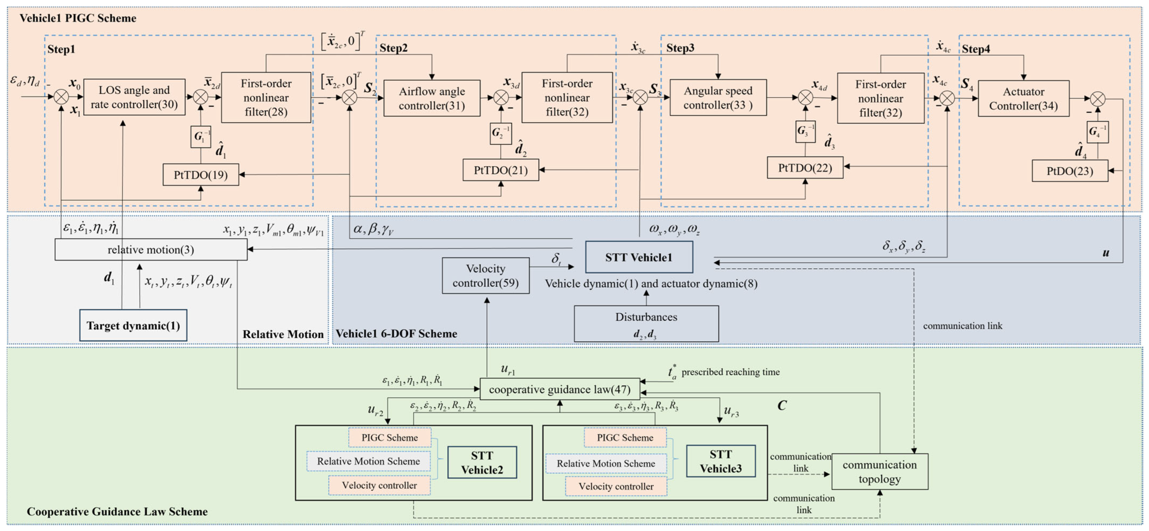
In this section, a three-dimensional CIGC scheme with global prescribed-time convergence is developed for the disturbed time-varying nonlinear fifth-order strict-feedback system (9), considering terminal angle constraints and actuator faults. The proposed design consists of four main parts: (1) In the Vehicle 1 6-DOF scheme, the thrust setting ${\delta }_t$ from the velocity controller and the actuator command $\mathit{u}$ from PIGC are taken as inputs, while the position $x_1$, $y_1$, $z_1$; velocity $V_{m1}$; attitude angles ${\theta }_{m1}$, ${\psi }_{V1}$, $\alpha$, $\beta$, ${\gamma }_V$; angular rates ${\omega }_x$, ${\omega }_y$, ${\omega }_z$, and actual control surface deflections ${\delta }_x$, ${\delta }_y$, ${\delta }_z$ are obtained as outputs. (2) In the relative motion scheme, the inputs are the information of the vehicle and the target, while the outputs include the relative distance $R_i(i=1,2,3)$, the LOS angle ${\epsilon }_i$ and ${\eta }_i$, and its derivative ${\dot{\epsilon }}_i$, ${\dot{\eta }}_i$, ${\dot{R}}_i$. (3) The Vehicle 1 PIGC scheme consists of four subsystems. It takes the inputs from (1) and (2) and generates the desired control command $\mathit{u}$. Four controllers are designed using prescribed-time sliding surfaces and reaching laws. A first-order nonlinear filter generates virtual commands for the airflow angle, angular rate, and actuator, along with their derivatives. Disturbances are handled via a prescribed-time disturbance observer. (4) In the cooperative guidance law design, based on the communication topology $\mathit{C}$ among the vehicles, the prescribed reaching time $t_a^{\ast }$, and the outputs of (2), the LOS direction acceleration command $u_{ri}$ is designed such that all vehicles achieve the same remaining flight time. The CIGC scheme structure is shown in Figure 2.

3.1. Preliminaries

The time-varying function $\phi (t_0,T)$ and $\mu (t_0,T)$ are defined as

$$\phi (t_0,T)\triangleq \left\{\begin{array}{l}{\displaystyle \frac{\dot{\mu }(t_0,T)}{\mu (t_0,T)}},t\in [t_0,t_0+T)\\ {\displaystyle \frac{p}{T}} ,t\in [T,\infty )\end{array}\right.$$

(10)

$$\mu (t_0,T)\triangleq \left\{\begin{array}{l}{\displaystyle \frac{T^p}{\left(T+t-t_0\right)}},t\in [t_0,t_0+T)\\ 1 ,t\in [T,\infty )\end{array}\right.$$

(11)

where $T>0$ denotes the prescribed convergence time and $p>1$ are design parameters. For $t=t_0$, $\phi (t_0,T)=1$ and as $t\to t_0+T$, $\phi (t_0,T)$ tends to infinity.

Definition 1.

Consider a nonlinear dynamic system

$$\dot{x}(t)=f(t,x(t)),x(0)=x_0$$

(12)

where $x(t)$ is the state vector and $f(t,x(t))$ is a nonlinear function related to $t$ and $x(t)$. System (12) is said to be prescribed-time stable at the origin if, for any initial condition $x(0)=x_0$, there exists a prescribed constant $T_C$ such that the solution $x(t,x_0)$ satisfies $x(t,x_0)=0$ for all $t\ge T_C$, and the settling time satisfies $T(x_0)<T_C$, where $T_C$ is the prescribed convergence time.

Definition 2.

Consider the sign function in vector form ${\mathit{x}}^{[m]}={[{\left|x_1\right|}^{m}sign(x_1),\dots ,{\left|x_n\right|}^{m}sign(x_n)]}^T$.

Lemma 1 ([38]).

For any real number $x_i,i=1,2\dots ,n$ , there exists a real number $0<q\le 1,p>1$such that

$$\left\{\begin{array}{l}{\displaystyle \sum _{i=1}^n{\left|x_i\right|}^p\ge {({\displaystyle \sum _{i=1}^n\left|x_i\right|})}^p}\\ {\displaystyle \sum _{i=1}^n{\left|x_i\right|}^q\ge n^{1-q}{({\displaystyle \sum _{i=1}^n\left|x_i\right|})}^q}\end{array}\right.$$

(13)

Lemma 2 ([39]).

For system (12), there exists a positive definite Lyapunov function $V(x)$ , $V(0)=0$ , such that for any solution $x(t,x_0)$ , it holds that

$$\dot{V}\le -{\displaystyle \frac{\pi }{\eta T_C}}(V^{1-\eta /2}+V^{1+\eta /2})+\xi$$

(14)

where $\eta \in (0,1)$, $T_C$ is a prescribed convergence time control parameter, and $\xi$ is a non-negative small constant. When $\xi =0$, the upper bound of the system convergence time is $T_C$. When $\xi \ne 0$, the system converges to a small neighbourhood, and the upper bound of the convergence time is $T_C/\sqrt{\mu }$, $0<\mu <1$. Then, one has

$$\underset{t\to T_C}{\lim }V\le \min \left\{{({\displaystyle \frac{\eta T_C\xi }{\pi (1-\mu )}})}^{{\displaystyle \frac{2}{2-\eta }}},{({\displaystyle \frac{\eta T_C\xi }{\pi (1-\mu )}})}^{{\displaystyle \frac{2}{2+\eta }}}\right\}$$

(15)

Lemma 3 ([40]).

For system (12), suppose that  $V(t,x(t)):U\times R_{+}\to R$ is a continuously differentiable function, where $U\subset R^m$ is an open neighbourhood containing the origin. If there exists a positive constant $b$ and $k$ such that

$$\begin{array}{l}V(t,0)=0,V(t,x(t))>0\\ \dot{V}=-bV-k\phi (t_0,T_p)V,t\ge t_0\end{array}$$

(16)

then system (12) is prescribed-time stable with the prescribed time $T_P$, and $V(t)$ satisfies

$$\left\{\begin{array}{l}V(t)\le \mu {(t_0,T)}^{-k}{\exp }^{-b(t-t_0)}V(t_0,x(t_0)),\hspace{0.33em}t\in [t_0,t_0+T_P)\hfill \\ V(t)\equiv 0,\hspace{0.33em}t\in [t_0+T_P,\infty ]\hfill \end{array}\right.$$

(17)

Theorem 1.

For system (12), there exists a positive definite Lyapunov function  $V(x)$:

$$\dot{V}(x)\le -{\alpha }_1{V}^q-a_{2}V-a_3{V}^p+\xi$$

(18)

where ${\alpha }_1>0$ , $a_2>0$ , $q>1$ , $p\in (0,1)$ , and $\xi$ is a non-negative small constant. When $\xi =0$ , according to [16], the upper bound of the system convergence time is $T_{\max }={\displaystyle \frac{1}{{\alpha }_2}}[{\displaystyle \frac{1}{(q-1)}}\ln (1+{\displaystyle \frac{{\alpha }_2}{{\alpha }_1}})+{\displaystyle \frac{1}{(1-p)}}\ln (1+{\displaystyle \frac{{\alpha }_2}{{\alpha }_3}})]$ . When $\xi \ne 0$ , the system converges to a small neighbourhood $\Omega =\left\{V\le 2{\gamma }_1|{\alpha }_1{\gamma }_1^q+a_2{\gamma }_1+a_3{\gamma }_1^p=\xi \right\}$ , and the upper bound of the convergence time is $T_{\max }={\displaystyle \frac{1}{{\alpha }_2}}[{\displaystyle \frac{1}{(q-1)}}\ln (1+{\displaystyle \frac{{\alpha }_2}{{\alpha }_1}})+{\displaystyle \frac{1}{(1-p)}}\ln (1+{\displaystyle \frac{{\alpha }_2}{{\alpha }_3(2^p-1)}})]$ . The proof of $\xi \ne 0$refers to Appendix A.1.

3.2. Prescribed-Time Disturbance Observer

For the disturbed system (9), a prescribed-time convergent disturbance observer is employed to estimate the disturbance. The prescribed-time disturbance observer (PtDO) used to estimate the disturbance ${\mathit{d}}_1$ is formulated as

$$\left\{\begin{array}{l}{\widehat{\dot{\mathit{x}}}}_1={\mathit{F}}_1+{\mathit{G}}_1{\overline{\mathit{x}}}_2+{\widehat{\mathit{d}}}_1-{\mathit{g}}_1{\mathit{e}}_1\\ {\dot{\widehat{\mathit{d}}}}_1=-{\mathit{g}}_2{\mathit{e}}_1\end{array}\right.$$

(19)

where ${\mathit{g}}_1$ and ${\mathit{g}}_2$ are time-varying functions, which are defined as

$$\left\{\begin{array}{l}{\mathit{g}}_1=l_1+2{\displaystyle \frac{l_3+2}{T_{Eso1}}}{\mu }_{T_{Eso1}}\\ {\mathit{g}}_2=l_2+l_1{\displaystyle \frac{l_3+2}{T_{Eso1}}}{\mu }_{T_{Eso1}}+{\displaystyle \frac{(l_3+2)(l_3+3)}{T_{Eso1}^2}}{\mu }_{T_{Eso1}}^2\end{array}\right.$$

(20)

where ${\widehat{\mathit{x}}}_1$ denotes the observed state, ${\widehat{\mathit{d}}}_1$ denotes the observed disturbance, ${\mathit{e}}_1={\mathit{x}}_1-{\widehat{\mathit{x}}}_1$. $l_1$, $l_2$ and $l_3$ are design parameters, which satisfy $\left[\begin{array}{cc}-l_1-{\displaystyle \frac{l_3+2}{T_{Eso1}}}{\mu }_{T_{Eso1}}& 1\\ -{\mathit{g}}_2& {\displaystyle \frac{l_3+2}{T_{Eso}}}{\mu }_{T_{Eso1}}\end{array}\right]$ is Hurwitz; therefore, $l_1>0$, $l_2>(2+l_3){({\displaystyle \frac{{\mu }_{TEso1}}{T_{Eso1}}})}^2$, $l_3>-2$. The prescribed convergence time of the disturbance observer is denoted by $T_{Eso1}$, and the definition of ${\mu }_{T_{Eso1}}$ is given in (11).

Lemma 4 ([23]).

By designing the prescribed-time disturbance observer as in (19), the observer estimation errors ${\tilde{\mathit{d}}}_1={\mathit{d}}_1-{\widehat{\mathit{d}}}_1$ will converge to the origin within the prescribed time $T_{Eso1}$.

The disturbance observer for ${\mathit{d}}_2$, ${\mathit{d}}_3$ and ${\mathit{d}}_4$ can be constructed as

$$\left\{\begin{array}{l}{\widehat{\dot{\mathit{x}}}}_2={\mathit{F}}_2+{\mathit{G}}_2{\mathit{x}}_3+{\mathit{k}}_{21}{\mathit{e}}_2^{[{\lambda }_{21}]}+{\mathit{k}}_{22}{\mathit{e}}_2^{[{\lambda }_{22}]}+{\displaystyle {\int }_0^t{\mathit{k}}_{23}\mathit{s}\mathit{i}\mathit{g}\mathit{n}({\mathit{e}}_2)dt}\\ {\widehat{\mathit{d}}}_2={\mathit{k}}_{21}{\mathit{e}}_2^{{\lambda }_{21}}+{\mathit{k}}_{22}{\mathit{e}}_2^{{\lambda }_{22}}+{\displaystyle {\int }_0^t{\mathit{k}}_{23}\mathit{s}\mathit{i}\mathit{g}\mathit{n}({\mathit{e}}_2)dt}\end{array}\right.$$

(21)

where ${\widehat{\mathit{x}}}_2$ denotes the observed state, ${\widehat{\mathit{d}}}_2$ denotes the observed disturbance, ${\mathit{e}}_2={\mathit{x}}_2-{\widehat{\mathit{x}}}_2$, ${\lambda }_{21}=1-{\eta }_{Eso2}$, ${\lambda }_{22}=1+{\eta }_{Eso2}$, ${\eta }_{Eso2}\in (0,1)$, ${\mathit{k}}_{21}={\displaystyle \frac{\pi }{{\eta }_{Eso2}{T}_{Eso2}}}{({\displaystyle \frac{1}{2}})}^{1-{\eta }_{Eso2}/2}$, ${\mathit{k}}_{22}={\displaystyle \frac{\pi }{{\eta }_{Eso2}{T}_{Eso2}}}{({\displaystyle \frac{1}{2}})}^{1-{\eta }_{Eso2}/2}$, and ${\mathit{k}}_{23}$ is greater than the upper bound of the disturbance rate of change. The prescribed convergence time of the disturbance observer is denoted by $T_{Eso2}$

$$\left\{\begin{array}{l}{\widehat{\dot{\mathit{x}}}}_3={\mathit{F}}_3+{\mathit{G}}_3{\mathit{x}}_4+{\mathit{k}}_{31}{\mathit{e}}_3^{[{\lambda }_{31}]}+{\mathit{k}}_{32}{\mathit{e}}_3^{[{\lambda }_{32}]}+{\displaystyle {\int }_0^t{\mathit{k}}_{33}\mathit{s}\mathit{i}\mathit{g}\mathit{n}({\mathit{e}}_3)dt}\\ {\widehat{\mathit{d}}}_3={\mathit{k}}_{31}{\mathit{e}}_3^{{\lambda }_{31}}+{\mathit{k}}_{32}{\mathit{e}}_3^{{\lambda }_{32}}+{\displaystyle {\int }_0^t{\mathit{k}}_{33}\mathit{s}\mathit{i}\mathit{g}\mathit{n}({\mathit{e}}_3)dt}\end{array}\right.$$

(22)

where ${\widehat{\mathit{x}}}_3$ denotes the observed state, ${\widehat{\mathit{d}}}_3$ denotes the observed disturbance, ${\mathit{e}}_3={\mathit{x}}_3-{\widehat{\mathit{x}}}_3$, ${\lambda }_{31}=1-{\eta }_{Eso3}$, ${\lambda }_{32}=1+{\eta }_{Eso3}$, ${\eta }_{Eso3}\in (0,1)$, ${\mathit{k}}_{31}={\displaystyle \frac{\pi }{{\eta }_{Eso3}{T}_{Eso3}}}{({\displaystyle \frac{1}{2}})}^{1-{\eta }_{Eso3}/2}$, ${\mathit{k}}_{32}={\displaystyle \frac{\pi }{{\eta }_{Eso3}{T}_{Eso3}}}{({\displaystyle \frac{1}{2}})}^{1-{\eta }_{Eso3}/2}$, and ${\mathit{k}}_{33}$ is greater than the upper bound of the disturbance rate of change. The prescribed convergence time of the disturbance observer is denoted by $T_{Eso3}$

$$\left\{\begin{array}{l}{\widehat{\dot{\mathit{x}}}}_4={\mathit{F}}_4+{\mathit{G}}_4\mathit{u}+{\mathit{k}}_{41}{\mathit{e}}_4^{[{\lambda }_{41}]}+{\mathit{k}}_{42}{\mathit{e}}_4^{[{\lambda }_{42}]}+{\displaystyle {\int }_0^t{\mathit{k}}_{43}\mathit{s}\mathit{i}\mathit{g}\mathit{n}({\mathit{e}}_4)dt}\\ {\widehat{\mathit{d}}}_4={\mathit{k}}_{41}{\mathit{e}}_4^{{\lambda }_{41}}+{\mathit{k}}_{42}{\mathit{e}}_4^{{\lambda }_{42}}+{\displaystyle {\int }_0^t{\mathit{k}}_{43}\mathit{s}\mathit{i}\mathit{g}\mathit{n}({\mathit{e}}_4)dt}\end{array}\right.$$

(23)

where ${\widehat{\mathit{x}}}_4$ denotes the observed state, ${\widehat{\mathit{d}}}_4$ denotes the observed disturbance, ${\mathit{e}}_4={\mathit{x}}_4-{\widehat{\mathit{x}}}_4$, ${\lambda }_{41}=1-{\eta }_{Eso4}$, ${\lambda }_{42}=1+{\eta }_{Eso4}$, ${\eta }_{Eso4}\in (0,1)$, ${\mathit{k}}_{41}={\displaystyle \frac{\pi }{{\eta }_{Eso4}{T}_{Eso4}}}{({\displaystyle \frac{1}{2}})}^{1-{\eta }_{Eso4}/2}$, ${\mathit{k}}_{42}={\displaystyle \frac{\pi }{{\eta }_{Eso4}{T}_{Eso4}}}{({\displaystyle \frac{1}{2}})}^{1-{\eta }_{Eso4}/2}$, and ${\mathit{k}}_{43}$ is greater than the upper bound of the disturbance rate of change. The prescribed convergence time of the disturbance observer is denoted by $T_{Eso4}$.

Theorem 2.

Define the disturbance observation error as ${\tilde{\mathit{d}}}_2={\mathit{d}}_2-{\widehat{\mathit{d}}}_2$ , ${\tilde{\mathit{d}}}_3={\mathit{d}}_3-{\widehat{\mathit{d}}}_3$ and ${\tilde{\mathit{d}}}_4={\mathit{d}}_4-{\widehat{\mathit{d}}}_4$ , and the derivatives of the disturbances satisfy $\left|{\dot{\mathit{d}}}_i\right|\le {\dot{\mathit{d}}}_{iMAX},i=2,3$ . Considering the nonlinear uncertain system (9) with the prescribed-time disturbance observer (19), the estimation error ${\tilde{\mathit{d}}}_i,i=2,3,4$ will converge to the origin within the prescribed time $T_{Esoi}$. The detailed proof of Theorem 2 is provided in Appendix A.2.

3.3. Global Prescribed-Time Sliding Mode IGC Law

Global prescribed-time convergence refers to the convergence of the observation errors ${\tilde{\mathit{d}}}_1$, ${\tilde{\mathit{d}}}_2$, ${\tilde{\mathit{d}}}_3$, ${\tilde{\mathit{d}}}_4$, the sliding surfaces ${\mathit{S}}_1$, ${\mathit{S}}_2={\mathit{x}}_2-{[{\overline{\mathit{x}}}_{2c},0]}^T$, ${\mathit{S}}_3={\mathit{x}}_3-{\mathit{x}}_{3c}$, and ${\mathit{S}}_4={\mathit{x}}_4-{\mathit{x}}_{4c}$, as well as the convergence of the state variables ${\mathit{x}}_1$ and ${\mathit{x}}_0$ to their desired values within the prescribed time. Therefore, Theorem 2 proves that the observation errors converge to their desired values within the prescribed time $T_{Eso}$. Subsequently, Theorem 3 proves that the sliding surfaces converge to their desired values within the prescribed time $T_{smc}$, while Theorem 4 proves that the state variables converge to their desired values within the prescribed time $T_{hit}$. Through the above techniques, global prescribed-time convergence is achieved.

To enable the vehicle to reach the target with the desired terminal angle, the guidance and control system is designed in an integrated manner based on sliding mode control combined with dynamic surface control. To ensure that the system states ${\mathit{x}}_0$ and ${\mathit{x}}_1$ converge to the origin within the prescribed time, a prescribed-time sliding surface is designed based on Lemma 3 as follows:

$${\mathit{S}}_1={\mathit{x}}_1+({\mathit{a}}_1+{\mathit{\lambda }}_1\phi (0,T_{hit})){\mathit{x}}_0$$

(24)

where ${\mathit{a}}_1$ and ${\mathit{\lambda }}_1$ are design parameters, which satisfy ${\mathit{a}}_1>0$, ${\mathit{\lambda }}_1>0$. $T_{hit}$ denotes the prescribed convergence time of the state variables ${\mathit{x}}_0$ and ${\mathit{x}}_1$.

Step 1: Design of the LOS angle and rate controller

Using the prescribed-time sliding surface in (24), the time derivative ${\mathit{S}}_1$ is obtained

$${\dot{\mathit{S}}}_1={\mathit{F}}_1+{\mathit{G}}_1{\overline{\mathit{x}}}_2+({\mathit{a}}_1+{\mathit{\lambda }}_1\phi (0,T_{hit})){\mathit{x}}_1+{\mathit{\lambda }}_1\dot{\phi }(0,T_{hit}){\mathit{x}}_0$$

(25)

To guarantee fast state convergence to the sliding surface, the prescribed-time reaching law is given by

$${\dot{\mathit{S}}}_{1c}=-({\mathit{\lambda }}_{S11}+{\mathit{\lambda }}_{S12}\phi (0,T_{gui})){\mathit{S}}_1-{\mathit{\lambda }}_{S13}{\mathit{S}}_1^{[m]}$$

(26)

where ${\mathit{S}}_1^{[m]}={[{\left|S_{11}\right|}^{m}sign(S_{11}),{\left|S_{12}\right|}^{m}sign(S_{12})]}^T$, $1>m>0$, ${\mathit{\lambda }}_{S11},{\mathit{\lambda }}_{S12},{\mathit{\lambda }}_{S13}$ are design parameters, which satisfy ${\mathit{\lambda }}_{S11,\min }>0,$ ${\mathit{\lambda }}_{S12,\min }>0$, ${\mathit{\lambda }}_{S13,\min }>0$. $T_{gui}$ denotes the prescribed convergence time of the sliding surface ${\mathit{S}}_1$.

Design the virtual control law ${\overline{\mathit{x}}}_{2d}$

$${\overline{\mathit{x}}}_{2d}={\mathit{G}}_1^{-1}(-{\mathit{F}}_1-{\widehat{\mathit{d}}}_1-({\mathit{a}}_1+{\mathit{\lambda }}_1\phi (0,T_{hit})){\mathit{x}}_1-{\mathit{\lambda }}_1\dot{\phi }(0,T_{hit}){\mathit{x}}_0-({\mathit{\lambda }}_{S11}+{\mathit{\lambda }}_{S12}\phi (0,T_{gui})){\mathit{S}}_1-{\mathit{\lambda }}_{S13}{\mathit{S}}_1^{[m]})$$

(27)

To avoid the differential explosion caused by repeated differentiation of virtual control inputs in high-order nonlinear systems, while ensuring prescribed-time convergence, a new virtual control law ${\overline{\mathit{x}}}_{2c}$ and its derivative ${\dot{\overline{\mathit{x}}}}_{2c}$ are obtained through a first-order nonlinear filter. This approach provides faster convergence and higher accuracy compared to a first-order low-pass filter. The filter is expressed as

$$\left\{\begin{array}{l}{\mathit{\tau }}_1{\dot{\overline{\mathit{x}}}}_{2c}=-{\mathit{y}}_1-{\mathit{y}}_1^{[a_1]}-{\mathit{y}}_1^{[a_2]}\\ {\overline{\mathit{x}}}_{2c}(0)={\overline{\mathit{x}}}_{2d}(0)\\ {\mathit{y}}_1={\overline{\mathit{x}}}_{2c}-{\overline{\mathit{x}}}_{2d}\end{array}\right.$$

(28)

where $a_1>1$ and $a_2\in (0,1)$; ${\mathit{\tau }}_1$ is design parameter.

The introduction of the filter causes a filter tracking error ${\mathit{y}}_1$. A compensation term ${\mathit{\xi }}_1$ is added to counteract the effect of the filter on the virtual control law.

$${\dot{\mathit{\xi }}}_i=\left\{\begin{array}{c}-{\mathit{l}}_i({\mathit{\xi }}_i+\phi (0,T_i){\mathit{\xi }}_i)-{\displaystyle \frac{{\mathit{\xi }}_i}{{‖{\mathit{\xi }}_i‖}^2}}{\mathit{s}}_i^T{\mathit{G}}_i{\mathit{y}}_i ,‖{\mathit{\xi }}_i‖>{\mu }_i\\ 0\hspace{1em}\hspace{1em}\hspace{1em}\hspace{1em}\hspace{1em}\hspace{1em}\hspace{1em}\hspace{1em}\hspace{1em}\hspace{1em}\hspace{1em}\hspace{1em},‖{\mathit{\xi }}_i‖\le {\mu }_i\end{array}\right. ,\mathrm{i}=1,2,3$$

(29)

where ${\mathit{l}}_i$ is a design parameter and ${\mu }_i$ is a small positive number selected to be as small as possible while maintaining system stability, and where ${\mathit{\xi }}_i$ denotes the compensation term associated with the $i$-th nonlinear filter. $T_1=T_{gui}$, $T_2=T_3=T_{smc}$.

At this point, ${\overline{\mathit{x}}}_{2d}$ is redefined as

$${\overline{\mathit{x}}}_{2d}={\mathit{G}}_1^{-1}(-{\mathit{F}}_1-{\widehat{\mathit{d}}}_1-({\mathit{a}}_1+{\mathit{\lambda }}_1\phi (0,T_{hit})){\mathit{x}}_1-{\mathit{\lambda }}_1\dot{\phi }(0,T_{hit}){\mathit{x}}_0-({\mathit{\lambda }}_{S11}+{\mathit{\lambda }}_{S12}\phi (0,T_{gui})){\mathit{S}}_1-{\mathit{\lambda }}_{S13}{\mathit{S}}_1^{[m]}-{\mathit{\xi }}_1)$$

(30)

Step 2: Design of the airflow angle controller

For STT vehicles, the desired ${\gamma }_V$ is set to zero. Define the errors ${\mathit{S}}_2={\mathit{x}}_2-{[{\overline{\mathit{x}}}_{2c},0]}^T$. Differentiating ${\mathit{S}}_2$ with respect to time yields ${\dot{\mathit{S}}}_2={\dot{\mathit{x}}}_2-{[{\dot{\overline{\mathit{x}}}}_{2c},0]}^T$.

Combining the prescribed-time reaching law and the compensation term ${\mathit{\xi }}_2$ to compensate for the filter-induced tracking error, the virtual control law is designed as

$${\mathit{x}}_{3d}={\mathit{G}}_2^{-1}(-{\mathit{F}}_2-{\widehat{\mathit{d}}}_2+{[{\dot{\overline{\mathit{x}}}}_{2c},0]}^T-({\mathit{\lambda }}_{S21}+{\mathit{\lambda }}_{S22}\phi (0,T_{smc})){\mathit{S}}_2-{\mathit{\lambda }}_{S23}{\mathit{S}}_2^{[m]}-\mathit{\chi }-{\mathit{\xi }}_2)$$

(31)

where $\mathit{\chi }=[{\mathit{G}}_1^T{\mathit{S}}_1{,0]}^T$, ${\mathit{S}}_2^{[m]}={[{\left|S_{21}\right|}^{m}sign(S_{21}),{\left|S_{22}\right|}^{m}sign(S_{22}),{\left|S_{23}\right|}^{m}sign(S_{23})]}^T$, ${\mathit{\lambda }}_{S21},{\mathit{\lambda }}_{S22}, {\mathit{\lambda }}_{S23}$ are design parameters, which satisfy ${\mathit{\lambda }}_{S21,\min }>0,$${\mathit{\lambda }}_{S22,\min }>0$,.${\mathit{\lambda }}_{S23,\min }>0$. $T_{smc}$ denotes the prescribed convergence time of the sliding surface.

Following Step 1, the nonlinear filter is employed to obtain the filtered virtual control ${\mathit{x}}_{3c}$ and its derivative ${\dot{\mathit{x}}}_{3c}$ as given by

$$\left\{\begin{array}{ll}{\mathit{\tau }}_i{\dot{\mathit{x}}}_{(i+1)c}=-{\mathit{k}}_{l1}{\mathit{y}}_i-{\mathit{y}}_i^{[a_1]}-{\mathit{y}}_i^{[a_2]}& \\ {\mathit{x}}_{(i+1)c}(0)={\mathit{x}}_{(i+1)d}(0)& \\ {\mathit{y}}_i={\mathit{x}}_{(i+1)c}-{\mathit{x}}_{(i+1)d}& ,i=2,3\end{array}\right.$$

(32)

where $a_1>1$ and $a_2\in (0,1)$; ${\mathit{\tau }}_i$ and ${\mathit{k}}_{l1}$ are the design parameters.

Step 3: Design of the angular speed controller

Define the errors ${\mathit{S}}_3={\mathit{x}}_3-{\mathit{x}}_{3c}$. Differentiating. ${\mathit{S}}_3$. with respect to time yields ${\dot{\mathit{S}}}_3={\dot{\mathit{x}}}_3-{\dot{\mathit{x}}}_{3c}$.

Combining the prescribed-time reaching law and the compensation term ${\mathit{\xi }}_3$ to compensate for the filter-induced tracking error, the virtual control law is designed as

$${\mathit{x}}_{4d}={\mathit{G}}_3^{-1}(-{\mathit{F}}_3-{\widehat{\mathit{d}}}_3+{\dot{\mathit{x}}}_{3c}-({\mathit{\lambda }}_{S31}+{\mathit{\lambda }}_{S32}\phi (0,T_{smc})){\mathit{S}}_3-{\mathit{\lambda }}_{S33}{\mathit{S}}_3^{[m]}-{\mathit{G}}_2^T{\mathit{S}}_2-{\xi }_3)$$

(33)

where ${\mathit{S}}_3^{[m]}={[{\left|S_{31}\right|}^{m}sign(S_{31}),{\left|S_{32}\right|}^{m}sign(S_{32}),{\left|S_{33}\right|}^{m}sign(S_{33})]}^T$, ${\mathit{\lambda }}_{S31},{\mathit{\lambda }}_{S32},{\mathit{\lambda }}_{S33}$ are design parameters, which satisfy ${\mathit{\lambda }}_{S31,\min }>0,$${\mathit{\lambda }}_{S32,\min }>0$, ${\mathit{\lambda }}_{S33,\min }>0$. $T_{smc}$ denotes the prescribed convergence time of the sliding surface ${\mathit{S}}_3$.

The filtered virtual control ${\mathit{x}}_{4c}$ and its derivative ${\dot{\mathit{x}}}_{4c}$ are obtained using the nonlinear filter in (32).

Step 4: Design of the actuator controller

Define the errors ${\mathit{S}}_4={\mathit{x}}_4-{\mathit{x}}_{4c}$. Differentiating ${\mathit{S}}_4$ with respect to time yields ${\dot{\mathit{S}}}_4={\dot{\mathit{x}}}_4-{\dot{\mathit{x}}}_{4c}$.

Combining the prescribed-time reaching law, the virtual control law is designed as

$$\mathit{u}={\mathit{G}}_4^{-1}(-{\mathit{F}}_4-{\widehat{\mathit{d}}}_4+{\dot{\mathit{x}}}_{4c}-({\mathit{\lambda }}_{S41}+{\mathit{\lambda }}_{S42}\phi (0,T_{smc})){\mathit{S}}_4-{\mathit{\lambda }}_{S43}{\mathit{S}}_4^{[m]})$$

(34)

where ${\mathit{S}}_4^{[m]}={[{\left|S_{41}\right|}^{m}sign(S_{41}),{\left|S_{42}\right|}^{m}sign(S_{42}),{\left|S_{43}\right|}^{m}sign(S_{43})]}^T$, ${\mathit{\lambda }}_{S41},{\mathit{\lambda }}_{S42},{\mathit{\lambda }}_{S43}$ are design parameters, which satisfy ${\mathit{\lambda }}_{S41,\min }>0$, ${\mathit{\lambda }}_{S42,\min }>0$, ${\mathit{\lambda }}_{S43,\min }>0$. $T_{smc}$ denotes the prescribed convergence time of the sliding surface ${\mathit{S}}_4$.

3.4. Stability Analysis

Theorem 3.

The prescribed-time control laws in (30), (31), (33) and (34) ensure that ${\mathit{S}}_1$ , ${\mathit{S}}_2$ , ${\mathit{S}}_3$ and ${\mathit{S}}_4$ converge to zero within the prescribed time $T_{smc}$.

Proof of Theorem 3.

$$\left\{\begin{array}{l}{\dot{\mathit{S}}}_1={\mathit{d}}_1-{\widehat{\mathit{d}}}_1+{\mathit{G}}_1({\overline{\mathit{S}}}_2+{\mathit{y}}_1)-({\mathit{\lambda }}_{S11}+{\mathit{\lambda }}_{S12}\phi (0,T_{gui})){\mathit{S}}_1-{\mathit{\lambda }}_{S13}{\mathit{S}}_1^{[m]}-{\mathit{\xi }}_1\\ {\dot{\mathit{S}}}_2={\mathit{d}}_2-{\widehat{\mathit{d}}}_2+{\mathit{G}}_2({\mathit{S}}_3+{\mathit{y}}_2)-({\mathit{\lambda }}_{S21}+{\mathit{\lambda }}_{S22}\phi (0,T_{smc})){\mathit{S}}_2-{\mathit{\lambda }}_{S23}{\mathit{S}}_2^{[m]}-{\mathit{\xi }}_2-\mathit{\chi }\\ {\dot{\mathit{S}}}_3={\mathit{d}}_3-{\widehat{\mathit{d}}}_3+{\mathit{G}}_3({\mathit{S}}_4+{\mathit{y}}_3)-({\mathit{\lambda }}_{S31}+{\mathit{\lambda }}_{S32}\phi (0,T_{smc})){\mathit{S}}_3-{\mathit{\lambda }}_{S33}{\mathit{S}}_3^{[m]}-{\mathit{\xi }}_3-{\mathit{G}}_2^T{\mathit{S}}_2\\ {\dot{\mathit{S}}}_4={\mathit{d}}_4-{\widehat{\mathit{d}}}_4-({\mathit{\lambda }}_{S41}+{\mathit{\lambda }}_{S42}\phi (0,T_{smc})){\mathit{S}}_4-{\mathit{\lambda }}_{S43}{\mathit{S}}_4^{[m]}\end{array}\right.$$

(35)

Define the Lyapunov function $\mathit{V}={\displaystyle \frac{1}{2}}({\mathit{S}}_1^T{\mathit{S}}_1+{\mathit{S}}_2^T{\mathit{S}}_2+{\mathit{S}}_3^T{\mathit{S}}_3+{\mathit{S}}_4^T{\mathit{S}}_4+{\mathit{\xi }}_1^T{\mathit{\xi }}_1+{\mathit{\xi }}_2^T{\mathit{\xi }}_2+{\mathit{\xi }}_3^T{\mathit{\xi }}_3)$, differentiating it with respect to time yields

$$\begin{array}{l}\dot{\mathit{V}}={\mathit{S}}_1^T\left({\mathit{d}}_1-{\widehat{\mathit{d}}}_1+{\mathit{G}}_1({\overline{\mathit{S}}}_2+{\mathit{y}}_1)-({\mathit{\lambda }}_{S11}+{\mathit{\lambda }}_{S12}\phi (0,T_{gui})){\mathit{S}}_1-{\mathit{\lambda }}_{S13}{\mathit{S}}_1^{[m]}-{\mathit{\xi }}_1\right)+{\mathit{\xi }}_1^T(-{\mathit{l}}_1({\mathit{\xi }}_1+\phi (0,T_{gui}){\mathit{\xi }}_1)\\ -{\displaystyle \frac{{\mathit{\xi }}_1}{{‖{\mathit{\xi }}_1‖}^2}}{\mathit{S}}_1^T{\mathit{G}}_1{\mathit{y}}_1)+{\mathit{S}}_2^T\left({\mathit{d}}_2-{\widehat{\mathit{d}}}_2+{\mathit{G}}_2({\mathit{S}}_3+{\mathit{y}}_2)-({\mathit{\lambda }}_{S21}+{\mathit{\lambda }}_{S22}\phi (0,T_{smc})){\mathit{S}}_2-{\mathit{\lambda }}_{S23}{\mathit{S}}_2^{[m]}-{[{\mathit{S}}_1^T{\mathit{G}}_1,0]}^T-{\mathit{\xi }}_2\right)\\ +{\mathit{\xi }}_2^T(-{\mathit{l}}_2({\mathit{\xi }}_2+\phi (0,T_{smc}){\mathit{\xi }}_2)-{\displaystyle \frac{{\mathit{\xi }}_2}{{‖{\mathit{\xi }}_2‖}^2}}{\mathit{S}}_2^T{\mathit{G}}_2{\mathit{y}}_2)+{\mathit{S}}_3^T({\mathit{d}}_3-{\widehat{\mathit{d}}}_3+{\mathit{G}}_3({\mathit{S}}_4+{\mathit{y}}_3)-({\mathit{\lambda }}_{S31}+{\mathit{\lambda }}_{S32}\phi (0,T_{smc})){\mathit{S}}_3\\ -{\mathit{\lambda }}_{S33}{\mathit{S}}_3^{[m]}-{\mathit{G}}_2^T{\mathit{S}}_2-{\mathit{\xi }}_3)+{\mathit{\xi }}_3^T(-{\mathit{l}}_3({\mathit{\xi }}_3+\phi (0,T_{smc}){\mathit{\xi }}_3)-{\displaystyle \frac{{\mathit{\xi }}_3}{{‖{\mathit{\xi }}_3‖}^2}}{\mathit{S}}_3^T{\mathit{G}}_3{\mathit{y}}_3)\\ +{\mathit{S}}_4^T({\mathit{d}}_4-{\widehat{\mathit{d}}}_4-({\mathit{\lambda }}_{S41}+{\mathit{\lambda }}_{S42}\phi (0,T_{smc})){\mathit{S}}_4-{\mathit{\lambda }}_{S43}{\mathit{S}}_4^{[m]})\end{array}$$

(36)

At $t\ge T_{Eso}$, according to Theorem 2, it follows that ${\tilde{\mathit{d}}}_i=0,i=1,2,3,4$.

$$\begin{array}{l}\dot{\mathit{V}}=-{\mathit{S}}_1^T({\mathit{\lambda }}_{S11}+{\mathit{\lambda }}_{S12}\phi (0,T_{gui})){\mathit{S}}_1-{\mathit{S}}_1^T{\mathit{\lambda }}_{S13}{\mathit{S}}_1^{[m]}-{\mathit{S}}_1^T{\mathit{\xi }}_1-{\mathit{l}}_1{\mathit{\xi }}_1^T({\mathit{\xi }}_1+\phi (0,T_{gui}){\mathit{\xi }}_1)\\ -{\mathit{S}}_2^T({\mathit{\lambda }}_{S21}+{\mathit{\lambda }}_{S22}\phi (0,T_{smc})){\mathit{S}}_2-{\mathit{S}}_2^T{\mathit{\lambda }}_{S23}{\mathit{S}}_2^{[m]}-{\mathit{S}}_2^T{\mathit{\xi }}_2-{\mathit{l}}_2{\mathit{\xi }}_2^T({\mathit{\xi }}_2+\phi (0,T_{smc}){\mathit{\xi }}_2)\\ +{\mathit{S}}_3^T{\mathit{G}}_3{\mathit{S}}_4-{\mathit{S}}_3^T({\mathit{\lambda }}_{S31}+{\mathit{\lambda }}_{S32}\phi (0,T_{smc})){\mathit{S}}_3-{\mathit{S}}_3^T{\mathit{\lambda }}_{S33}{\mathit{S}}_3^{[m]}-{\mathit{S}}_3^T{\mathit{\xi }}_3-{\mathit{l}}_3{\mathit{\xi }}_3^T({\mathit{\xi }}_3+\phi (0,T_{smc}){\mathit{\xi }}_3)\\ +{\mathit{S}}_4^T(-({\mathit{\lambda }}_{S41}+{\mathit{\lambda }}_{S42}\phi (0,T_{smc}))S_4-{\mathit{\lambda }}_{S43}{\mathit{S}}_4^{[m]})\end{array}$$

(37)

According to Young’s inequality, it yields

$$\begin{array}{l}\dot{\mathit{V}}\le -[{\mathit{S}}_1^T({\mathit{\lambda }}_{S11}-{\displaystyle \frac{1}{2\epsilon }}\mathit{I}){\mathit{S}}_1+{\mathit{S}}_2^T({\mathit{\lambda }}_{S21}-{\displaystyle \frac{1}{2\epsilon }}\mathit{I}){\mathit{S}}_2+{\mathit{S}}_3^T({\mathit{\lambda }}_{S31}-{\displaystyle \frac{1}{2}}{\mathit{G}}_3{\mathit{G}}_3^T-{\displaystyle \frac{1}{2\epsilon }}\mathit{I}){\mathit{S}}_3\\ +{\mathit{S}}_4^T({\mathit{\lambda }}_{S41}-{\displaystyle \frac{1}{2\epsilon }}\mathit{I}+){\mathit{S}}_4+({\mathit{l}}_1-{\displaystyle \frac{\epsilon }{2}}\mathit{I}){\mathit{\xi }}_1^T{\mathit{\xi }}_1+({\mathit{l}}_2-{\displaystyle \frac{\epsilon }{2}}\mathit{I}){\mathit{\xi }}_2^T{\mathit{\xi }}_2+({\mathit{l}}_3-{\displaystyle \frac{\epsilon }{2}}\mathit{I}){\mathit{\xi }}_3^T{\mathit{\xi }}_3]\\ -[{\mathit{S}}_1^T{\mathit{\lambda }}_{S12}\phi (0,T_{gui}){\mathit{S}}_1+{\mathit{S}}_2^T{\mathit{\lambda }}_{S22}\phi (0,T_{smc}){\mathit{S}}_2+{\mathit{S}}_3^T{\mathit{\lambda }}_{S32}\phi (0,T_{smc}){\mathit{S}}_3+{\mathit{S}}_4^T{\mathit{\lambda }}_{S42}\phi (0,T_{smc}){\mathit{S}}_4\\ +{\mathit{l}}_1{\mathit{\xi }}_1^T\phi (0,T_{gui}){\mathit{\xi }}_1+{\mathit{l}}_2{\mathit{\xi }}_2^T\phi (0,T_{smc}){\mathit{\xi }}_2+{\mathit{l}}_3{\mathit{\xi }}_3^T\phi (0,T_{smc}){\mathit{\xi }}_3]\end{array}$$

(38)

The parameters are chosen such that

$$\begin{array}{l}{\mathit{\lambda }}_{S11}\ge (b+{\displaystyle \frac{1}{2\epsilon }})\mathit{I},{\mathit{\lambda }}_{S12}\ge k,{\mathit{\lambda }}_{S13}\ge k,b>0,\epsilon \ge 2,k>0\\ {\mathit{\lambda }}_{S21}\ge (b+{\displaystyle \frac{1}{2\epsilon }})\mathit{I},{\mathit{\lambda }}_{S22}\ge k,{\mathit{\lambda }}_{S23}\ge 0,\\ {\mathit{\lambda }}_{S31}\ge (b+{\displaystyle \frac{1}{2\epsilon }}+{\displaystyle \frac{1}{2}}{\mathit{G}}_3{\mathit{G}}_3^T)\mathit{I},{\mathit{\lambda }}_{S32}\ge k,{\mathit{\lambda }}_{S33}\ge 0,\\ {\mathit{\lambda }}_{S41}\ge (b+{\displaystyle \frac{1}{2\epsilon }})\mathit{I},{\mathit{\lambda }}_{S42}\ge k,{\mathit{\lambda }}_{S43}\ge 0,\\ {\mathit{l}}_1\ge ({\displaystyle \frac{\epsilon }{2}}+b)\mathit{I},{\mathit{l}}_2\ge ({\displaystyle \frac{\epsilon }{2}}+b)\mathit{I},{\mathit{l}}_3\ge ({\displaystyle \frac{\epsilon }{2}}+b)\mathit{I},T_{hit}=T_{smc}\end{array}$$

(39)

Substituting (39) into (38) yields

$$\begin{array}{l}\dot{\mathit{V}}\le -b[{\mathit{S}}_1^T{\mathit{S}}_1+{\mathit{S}}_2^T{\mathit{S}}_2+{\mathit{S}}_3^T{\mathit{S}}_3+{\mathit{S}}_4^T{\mathit{S}}_4+{\mathit{\xi }}_1^T{\mathit{\xi }}_1+{\mathit{\xi }}_2^T{\mathit{\xi }}_2+{\mathit{\xi }}_3^T{\mathit{\xi }}_3]-k[{\mathit{S}}_1^T\phi (0,T_{smc}){\mathit{S}}_1+{\mathit{S}}_2^T\phi (0,T_{smc}){\mathit{S}}_2\\ +{\mathit{S}}_3^T\phi (0,T_{smc}){\mathit{S}}_3+{\mathit{S}}_4^T\phi (0,T_{smc}){\mathit{S}}_4+({\displaystyle \frac{\epsilon }{2}}+b){\mathit{\xi }}_1^T\phi (0,T_{smc}){\mathit{\xi }}_1+({\displaystyle \frac{\epsilon }{2}}+b){\mathit{\xi }}_2^T\phi (0,T_{smc}){\mathit{\xi }}_2\\ +({\displaystyle \frac{\epsilon }{2}}+b){\mathit{\xi }}_3^T\phi (0,T_{smc}){\mathit{\xi }}_3]\\ \le -b[{\mathit{S}}_1^T{\mathit{S}}_1+{\mathit{S}}_2^T{\mathit{S}}_2+{\mathit{S}}_3^T{\mathit{S}}_3+{\mathit{S}}_4^T{\mathit{S}}_4+{\mathit{\xi }}_1^T{\mathit{\xi }}_1+{\mathit{\xi }}_2^T{\mathit{\xi }}_2+{\mathit{\xi }}_3^T{\mathit{\xi }}_3]\\ -k[{\mathit{S}}_1^T\phi (0,T_{smc}){\mathit{S}}_1+{\mathit{S}}_2^T\phi (0,T_{smc}){\mathit{S}}_2+{\mathit{S}}_3^T\phi (0,T_{smc}){\mathit{S}}_3\\ +{\mathit{S}}_4^T\phi (0,T_{smc}){\mathit{S}}_4+{\mathit{\xi }}_1^T\phi (0,T_{smc}){\mathit{\xi }}_1+{\mathit{\xi }}_2^T\phi (0,T_{smc}){\mathit{\xi }}_2+{\mathit{\xi }}_3^T\phi (0,T_{smc}){\mathit{\xi }}_3]\\ \le -2b\mathit{V}-2k\phi (0,T_{smc})\mathit{V}\end{array}$$

(40)

The parameter selection satisfies (39), and by Lemma 3, ${\mathit{S}}_1$, ${\mathit{S}}_2$, ${\mathit{S}}_3$, and ${\mathit{S}}_4$ reach the origin within the prescribed time $T_{smc}$. □

Theorem 4.

With the control law designed in (30), the LOS angle error and its rate converge to the sliding surface (24) within the prescribed time  $T_{gui}$ , and both the LOS angle error and its rate reach zero at the prescribed time $T_{hit}$.

Proof of Theorem 4.

When the state variables are on the sliding surface,

$${\mathit{S}}_1={\mathit{x}}_1+({\mathit{a}}_1+{\mathit{\lambda }}_1\phi (0,T_{hit})){\mathit{x}}_0=0$$

(41)

Define the Lyapunov function ${\mathit{V}}_{x0}={\displaystyle \frac{1}{2}}{\mathit{x}}_0^T{\mathit{x}}_0$. Its time derivative is given by

$$\begin{array}{c}{\dot{\mathit{V}}}_{\mathit{x}0}={\mathit{x}}_0^T{\dot{\mathit{x}}}_0=-{\mathit{x}}_0^T({\mathit{a}}_1+{\mathit{\lambda }}_1\phi (0,T_{hit})){\mathit{x}}_0\\ \le -2{\mathit{a}}_1{\mathit{V}}_{x0}-2{\mathit{\lambda }}_1\phi (0,T_{hit}){\mathit{V}}_{x0}\end{array}$$

(42)

The parameters are chosen such that

$${\mathit{a}}_1>0,{\mathit{\lambda }}_1>0$$

(43)

By Lemma 3, ${\mathit{x}}_0$ reach the origin within the prescribed time $T_{hit}$.

From the above derivations, the observer estimation error converges to zero within the prescribed time $T_{Eso}$, while the tracking errors of the airflow angle, angular rate, and fin deflection converge within $T_{smc}$. The LOS angle error and its derivative reach the sliding surface in $T_{gui}$ and both become zero at $T_{hit}$. To ensure prescribed-time convergence, the prescribed-time parameter should satisfy $T_{Eso}<T_{smc}=T_{gui}<T_{hit}$. □

3.5. Cooperative Guidance Law

First, some relevant graph theory concepts are introduced. During the mission, vehicles can be regarded as multiple agents, and their communication is described using graph theory. An undirected graph $\mathit{G}=\left\{\mathit{V},\mathit{E},\mathit{C}\right\}$ is used, where $\mathit{V}=\left\{v_i,i=1,2,\dots ,n\right\}$ represents the set of nodes and $\mathit{E}\subseteq \mathit{V}\times \mathit{V}$ represents the set of edges, i.e., communication links between two nodes. The adjacency matrix $\mathit{C}=\left[c_{ij}\right]\in {\mathit{R}}^{n\times n}$ represents the connectivity: if nodes $v_i$ and $v_j$ can communicate, then $c_{ij}=c_{ji}=1$; otherwise, $c_{ij}=c_{ji}=0$, for all $i\in V$, $c_{ii}=0$. Hence, $\mathit{C}$ is a non-negative symmetric matrix. A path from node $v_i$ to node $v_j$ in the graph is a sequence of distinct vertices with $v_i$ as the start and $v_j$ as the end, where consecutive vertices are connected. If there exists a path between any two vertices in the graph, the graph is said to be connected. The Laplacian matrix ${\mathit{L}}_C=[l_{ij}]$ is defined as $l_{ii}={\displaystyle \sum _{j=1}^n{c}_{ij}}$ and $l_{ij}=-c_{ij}$ for $i\ne j$.

Based on the engagement model in (3), the design model of the cooperative guidance law can be derived as

$$\left\{\begin{array}{l}{\dot{x}}_1=x_2\\ {\dot{x}}_2=x_1{\dot{\epsilon }}^2+x_1{\dot{\eta }}^2{\cos }^2\epsilon -u_r+a_{Tr}\end{array}\right.$$

(44)

where $x_1=R$, $x_2=\dot{R}$. $u_r$ and $a_{Tr}$ represent the components of the accelerations of the vehicle and the target along the LOS. $a_{Tr}$ is bounded, such that $\left|a_{Tr}\right|\le {\delta }^{\ast }$, where ${\delta }^{\ast }$ is a positive constant.

Introduce the remaining time-to-go $t_{goi}$ for the terminal guidance of the $i$ vehicle,

$$t_{goi}=-{\displaystyle \frac{R_i}{{\dot{R}}_i}}=-{\displaystyle \frac{x_{1i}}{x_{2i}}}$$

(45)

Differentiating (45) yields

$${\dot{t}}_{goi}=-1+{\displaystyle \frac{x_{1i}^2{\dot{\epsilon }}_i^2}{x_{2i}^2}}+{\displaystyle \frac{x_{1i}^2{\dot{\eta }}_i^2{\cos }^2\epsilon }{x_{2i}^2}}-{\displaystyle \frac{x_{1i}}{x_{2i}^2}}{u}_{ri}+{\displaystyle \frac{x_{1i}}{x_{2i}^2}}{a}_{Tri}$$

(46)

The reaching time of each vehicle is $t_{ai}=t_{goi}+t$. Achieving consensus on the remaining time-to-go $t_{goi}$ ensures that the arrival times $t_{ai}$ are aligned, so all vehicles arrive at the target simultaneously. Inspired by [37], an adaptive cooperative guidance law with faster fixed-time convergence is designed. The system described in Theorem 1 achieves a faster convergence rate than system $\dot{V}(x)\le -{\alpha }_1{V}^q-a_2{V}^p$[16].

$$\left\{\begin{array}{l}{u}_{ri}={\displaystyle \frac{x_{2i}^2}{x_{1i}}}\left\{\begin{array}{l}{\displaystyle \frac{x_{1i}^2{\epsilon }_i^2}{x_{2i}^2}}+{\displaystyle \frac{x_{1i}^2{\dot{\eta }}_i^2{\cos }^2{\epsilon }_i}{x_{2i}^2}}+{\delta }_{ri}sat\left(t_{ai}-t_a^{\ast }\right)-{\alpha }_1{\displaystyle \sum _{j\in {\mathcal{N}}_i}{c}_{ij}}{\left(t_{goj}-t_{goi}\right)}^{q_1}\\ -{\alpha }_2{\displaystyle \sum _{j\in {\mathcal{N}}_i}{c}_{ij}}\left(t_{goj}-t_{goi}\right)-{\alpha }_3{\displaystyle \sum _{j\in {\mathcal{N}}_i}{c}_{ij}}{\left(t_{goj}-t_{goi}\right)}^{p_1}\end{array}\right\}\\ {\dot{\delta }}_{ri}={\chi }_1\left|t_{ai}-t_a^{\ast }\right|\end{array}\right.$$

(47)

where ${\alpha }_1$, ${\alpha }_2$, ${\alpha }_3$, $p_1$, $q_1$ are scalars satisfying $p_1/q_1<1$; ${\delta }_{ri}$ is an adaptive gain, ${\chi }_1$ is a positive constant, and $t_a^{\ast }$ denotes the prescribed arrival time. Since the use of the sign function may lead to system chattering, the saturation function (sat) is introduced to replace it.

$$sat\left(t_{ai}-t_a^{\ast }\right)=\left\{\begin{array}{l}1,t_{ai}-t_a^{\ast }>\delta \\ {\displaystyle \frac{t_{ai}-t_a^{\ast }}{\delta }},-\delta \le t_{ai}-t_a^{\ast }\le \delta \\ -1,t_{ai}-t_a^{\ast }<-\delta \end{array}\right.$$

(48)

Theorem 5.

For the $i$ vehicle system (44), assuming an undirected and connected communication topology $\mathit{C}$ , the adaptive guidance law (47) ensures that the arrival time error $e_i=t_{ai}-t_a^{\ast }$ achieves fixed-time consensus, with $T_r$ as the state-free settling time $\underset{t\to T_r}{\lim }\left|e_i\right|=\underset{t\to T_r}{\lim }\left|t_{ai}-t_a^{\ast }\right|\le {\Theta }_1$ and ${\Theta }_1$ as a tuneable bound. Therefore, the remaining flight times $t_{goi}$ converge to consensus within a bounded time. The detailed proof of Theorem 5 is provided in Appendix A.3.

$$T_r={\displaystyle \frac{1}{2{\alpha }_2\tilde{\lambda }}}[{\displaystyle \frac{1}{(q-1)}}\ln (1+{\displaystyle \frac{4{\alpha }_2\tilde{\lambda }}{{\alpha }_1{n}^{1-q_1}{(4\tilde{\lambda })}^{\frac{q_1+1}{2}}}})+{\displaystyle \frac{1}{(1-p)}}\ln (1+{\displaystyle \frac{4{\alpha }_2\tilde{\lambda }}{{\alpha }_3{(4\tilde{\lambda })}^{\frac{p_1+1}{2}}(2^p-1)}})]$$

(49)

3.6. Prescribed-Time Convergence Velocity Controller Design

${\dot{V}}_{cmd}=u_{ri}$ denotes the vehicle acceleration command. The engine model is defined as follows:

$$\left\{\begin{array}{l}{P}_{cmd}=P_{ref}{\delta }_t{\displaystyle \frac{\rho }{{\rho }_0}}(1-k_{v}Mach)\\ P+\tau \dot{P}=P_{cmd}\end{array}\right.$$

(50)

where $P_{cmd}$ denotes the desired thrust, $P$ represents the actual thrust after the first-order inertial dynamics $\tau$, $P_{ref}$ is the reference maximum thrust, ${\delta }_t\in [0,1]$ denotes the thrust setting, ${\displaystyle \frac{\rho }{{\rho }_0}}$ is the density ratio which reflects the attenuation of thrust caused by thin air at high altitudes, $\rho$ stands for the air density at the current flight altitude, ${\rho }_0=1.225 \mathrm{k}\mathrm{g}/{\mathrm{m}}^3$ is the standard sea-level air density, $k_v$ is the velocity correction coefficient characterizing the effect of flight speed on thrust, and $Mach$ denotes the flight Mach number.

For the design of the velocity controller, by combining (1) and (50), the following nonlinear dynamic equation is established as

$$\left\{\begin{array}{l}{\dot{\overline{x}}}_1={\overline{f}}_1+{\overline{g}}_1{\overline{x}}_2\\ {\dot{\overline{x}}}_2={\overline{f}}_2+{\overline{g}}_{2}u\end{array}\right.$$

(51)

where ${\overline{f}}_1={\displaystyle \frac{-X-mg\sin {\theta }_m}{m}}$, ${\overline{g}}_1={\displaystyle \frac{\cos \alpha \cos \beta }{m}}$, ${\overline{f}}_2=-{\displaystyle \frac{P}{\tau }}$, ${\overline{g}}_2=-{\displaystyle \frac{1}{\tau }}$, ${\overline{x}}_1=V$, ${\overline{x}}_2=P$, $u=P_{ref}{\delta }_t{\displaystyle \frac{\rho }{{\rho }_0}}(1-k_{v}Mach)$.

Design a velocity controller for each vehicle based on the backstepping control method and define the tracking error $e_1=V-V_{cmd}={\overline{x}}_1-{\overline{x}}_{1cmd}$. Differentiating $e_1$ yields ${\dot{e}}_1=\dot{V}-{\dot{V}}_{cmd}$. Combined with the prescribed-time convergence law, the following expression is obtained

$$S_{5c}=-({\lambda }_{S51}+{\lambda }_{S52}\phi (0,T_{vel}))e_1-{\lambda }_{S53}{e}_1^{[m]}$$

(52)

$${\overline{x}}_{2d}={\overline{g}}_1^{-1}(S_{5c}-f_1+{\dot{\overline{x}}}_{1cmd})$$

(53)

where ${\lambda }_{S51},{\lambda }_{S52},{\lambda }_{S53}$ are design parameters. $T_{vel}$ denotes the prescribed convergence time of the error $e_1$.

To avoid the differential explosion caused by repeated differentiation of virtual control inputs in high-order nonlinear systems, a new virtual control law ${\overline{x}}_{2c}$ and its derivative ${\dot{\overline{x}}}_{2c}$ are obtained through a first-order nonlinear filter. The filter is expressed as

$$\left\{\begin{array}{l}{\tau }_4{\dot{\overline{x}}}_{2c}=-k_{l1}{y}_4-y_4^{[a_1]}-y_4^{[a_2]}\\ P_c(0)=P_d(0)\\ y_4={\overline{x}}_{2c}-{\overline{x}}_{2d}\end{array}\right.$$

(54)

where $a_1>1$ and $a_2\in (0,1)$, ${\tau }_4$, $k_{l1}$ are design parameters.

The introduction of the filter causes a filter tracking error $y_4$. A compensation term ${\mathit{\xi }}_4$ is added to counteract the effect of the filter on the virtual control law.

$${\dot{\mathit{\xi }}}_4=\left\{\begin{array}{l}-l_4({\mathit{\xi }}_4+\phi (0,T_{vel}){\mathit{\xi }}_4)-{\displaystyle \frac{{\mathit{\xi }}_4}{{‖{\mathit{\xi }}_4‖}^2}}{\overline{\mathrm{g}}}_1{e}_1{y}_4 ,‖{\mathit{\xi }}_4‖>{\mu }_4\\ 0\hspace{1em}\hspace{1em}\hspace{1em}\hspace{1em}\hspace{1em}\hspace{1em}\hspace{1em}\hspace{1em}\hspace{1em}\hspace{1em}\hspace{1em}\hspace{1em}\hspace{1em},‖{\mathit{\xi }}_4‖\le {\mu }_4\end{array}\right.$$

(55)

where $l_4$ is a design parameter and ${\mu }_4$ is a small positive number.

$${\overline{x}}_{2d}={\overline{g}}_1^{-1}(S_{5c}-f_1+{\dot{\overline{x}}}_{1cmd}-{\xi }_4)$$

(56)

Define the tracking error $e_2=P-P_c={\overline{x}}_2-{\overline{x}}_{2c}$. Differentiating $e_2$ yields ${\dot{e}}_2={\dot{\overline{x}}}_2-{\dot{\overline{x}}}_{2c}$. Combined with the prescribed-time convergence law, the following expression is obtained

$$S_{6c}=-({\lambda }_{S61}+{\lambda }_{S62}\phi (0,T_{vel}))e_2-{\lambda }_{S63}{e}_2^{[m]}$$

(57)

$$u={\overline{g}}_2^{-1}(S_{6c}+{\dot{\overline{x}}}_{2c}-{\overline{f}}_2-e_1{\overline{g}}_1)$$

(58)

where ${\lambda }_{S61},{\lambda }_{S62},{\lambda }_{S63}$ are design parameters. $T_{vel}$ denotes the prescribed convergence time of the error $e_2$.

Thus, the throttle command is given by

$${\delta }_t={\displaystyle \frac{u{\rho }_0}{P_{ref}\rho (1-k_{v}Mach)}}$$

(59)

Theorem 6.

For the vehicle velocity control, (59) ensures that the vehicle velocity converges to the desired velocity within the prescribed time $T_{vel}$. The detailed proof of Theorem 6 is provided in Appendix A.4.

4. Numerical Simulations

This section first introduces the simulation environment and parameter settings. Five simulation cases are conducted to validate the performance of the proposed algorithm. In Case 1, a single vehicle approaches a moving target with a desired terminal angle, and its performance is compared to two existing algorithms to demonstrate the superiority of the proposed algorithm. In Case 2, sensor noise and state-estimation errors are introduced based on Case 1, together with more severe actuator faults, to further evaluate the robustness of the proposed algorithm. In Case 3, multiple vehicles are launched from different initial positions to cooperatively approach a moving target under specified desired terminal angle constraints, thereby verifying the effectiveness of the proposed algorithm. In Case 4, communication failure is introduced among three vehicles, where communication information can only be transmitted in one direction, to validate the effectiveness of the proposed algorithm under communication failure conditions. In Case 5, aerodynamic parameter uncertainties are introduced through Monte Carlo simulations. Multiple vehicles are launched from widely separated initial positions to cooperatively approach a moving target under randomly assigned desired terminal angle constraints, demonstrating the robustness of the proposed algorithm. Cases 1, 3, 4, and 5 are conducted without considering sensor noise or biases.

4.1. Simulation Setup and Parameters

The simulation is performed using the ode 4 solver with a fixed-step size of 0.001 s. The CIGC design parameters, vehicle aerodynamic parameters, and initial states are listed in

Table 3. Parameter selection for the first-order nonlinear filter and filter compensation term.

	${\mathit{\tau }}_1$	${\mathit{\tau }}_2$	${\mathit{\tau }}_3$	${\mathit{\tau }}_4$	${\mathit{a}}_1$	${\mathit{a}}_2$	${\mathit{l}}_1, {\mathit{l}}_2, {\mathit{l}}_3, {\mathit{l}}_4$	${\mathit{\mu }}_{\mathit{i}}(\mathit{i} = 1, 2, 3, 4)$
Vehicles 1–3	$\mathrm{diag}(0.1,0.1)$	$\mathrm{diag}(0.1,0.1,0.1)$	$\mathrm{diag}(0.1,0.1,0.1)$	$0.1$	$9/7$	$7/9$	2	0.01

,

Table 4. Parameter selection for the prescribed-time convergent disturbance observer.

	${\mathit{T}}_{\mathit{E}\mathit{s}\mathit{o}1,2,3,4}(\mathit{s})$	${\mathit{l}}_1$	${\mathit{l}}_2$	${\mathit{l}}_3$	${\mathit{\eta }}_{\mathit{E}\mathit{s}\mathit{o}2\mathit{,}3\mathit{,}4}$	${\mathit{k}}_{23}$	${\mathit{k}}_{33}$	${\mathit{k}}_{43}$
Vehicles 1–3	5	$1$	$1$	$0.3$	$0.05$	$\mathrm{diag}(0.1,0.1,0.1)$	$\mathrm{diag}(0.1,0.1,0.1)$	$\mathrm{diag}(0.1,0.1,0.1)$

,

Table 5. Parameter selection for the LOS controller.

	${\mathit{T}}_{\mathit{g}\mathit{u}\mathit{i}}(\mathit{s})$	${\mathit{T}}_{\mathit{h}\mathit{i}\mathit{t}}(\mathit{s})$	${\mathit{a}}_1$	${\mathit{\lambda }}_1$	${\mathit{\lambda }}_{\mathit{S}11}$	${\mathit{\lambda }}_{\mathit{S}12}$	${\mathit{\lambda }}_{\mathit{S}13}$	$\mathit{m}$	$\mathit{p}$
Vehicles 1–3	8	12	$\mathrm{diag}(0.2,0.2)$	$\mathrm{diag}(2,2)$	$\mathrm{diag}(0.2,0.2)$	$\mathrm{diag}(1,1)$	$\mathrm{diag}(0.1,0.1)$	$7/9$	2

,

Table 6. Parameter selection for the airflow angle, angle rate, actuator controller.

	${\mathit{T}}_{smc}(\mathit{s})$	${\mathit{\lambda }}_{S21},{\mathit{\lambda }}_{S31},{\mathit{\lambda }}_{S41}$	${\mathit{\lambda }}_{S22},{\mathit{\lambda }}_{S32},{\mathit{\lambda }}_{S42}$	${\mathit{\lambda }}_{S23},{\mathit{\lambda }}_{S33},{\mathit{\lambda }}_{S43}$	$\mathit{m}$
Vehicles 1–3	8	$5,1,1$	$2,1,2$	$5,1,2$	$7/9$

,

Table 7. Parameter selection for cooperative guidance law.

	${\mathit{\alpha }}_{1,2,3}$	${\mathit{p}}_1$	${\mathit{q}}_1$	${\mathit{\chi }}_1$	${\mathit{t}}_{\mathit{a}}^{\ast }(\mathit{s})$
Vehicles 1–3	0.001	0.714	1.286	0.005	18

,

Table 8. Parameter selection for velocity controller.

	${\mathit{\lambda }}_{\mathit{S}51}$	${\mathit{\lambda }}_{\mathit{S}61}$	${\mathit{\lambda }}_{\mathit{S}52,62}$	${\mathit{\lambda }}_{\mathit{S}53,63}$	$\mathit{m}$	${\mathit{T}}_{\mathit{v}\mathit{e}\mathit{l}}(\mathit{s})$	${\mathit{k}}_{\mathit{v}}$	$\mathit{\tau }$
Vehicles 1–3	8	5	1	1	$7/9$	5	0.15	0.05

,

Table 9. The initial flight parameters of the vehicle.

	$\mathit{x}(\mathit{m})$	$\mathit{y}(\mathit{m})$	$\mathit{z}(\mathit{m})$	$\mathit{V}(\mathit{m}/\mathit{s})$	$\mathit{\theta }(\circ )$	$\mathit{\psi }(\circ )$	${\mathit{h}}_{\mathit{x}},{\mathit{h}}_{\mathit{y}},{\mathit{h}}_{\mathit{z}}$	${\mathit{\upsilon }}_{\mathit{x}},{\mathit{\upsilon }}_{\mathit{y}},{\mathit{\upsilon }}_{\mathit{z}}(\circ )$	$\mathit{\xi }$
Vehicle 1	0	5000	500	300	0.573	0	0.8	0.1	0.05
Vehicle 2	200	5000	400	300	0.573	0	0.8	0.1	0.05
Vehicle 3	−300	4500	500	300	0.573	0	0.8	0.1	0.05
Target	3000	0	0	20	20	0

and

Table 10. Vehicle aerodynamic parameters.

Parameter	Value	Parameter	Value	Parameter	Value	Parameter	Value	Parameter	Value
$S({\mathrm{m}}^2)$	0.3	$J_z(\mathrm{K}\mathrm{g}.{\mathrm{m}}^2)$	560	$c_x^{\delta y}$	0.07	$c_z^{\beta }$	−25.31	$m_y^{\delta y}$	−10.97
$L\left(\mathrm{m}\right)$	2.4	$c_{x0}$	0.32	$c_x^{\delta z}$	0.06	$m_x^{\alpha }$	0.46	$m_z^{\alpha }$	−1.61
$m(\mathrm{K}\mathrm{g})$	253	$c_x^{\alpha }$	0.21	$c_y^{\alpha }$	25.16	$m_x^{\beta }$	−0.37	$m_z^{\delta z}$	−10.92
$J_x(\mathrm{K}\mathrm{g}.{\mathrm{m}}^2)$	100	$c_x^{\beta }$	0.19	$c_y^{\beta }$	−0.08	$m_x^{\delta x}$	2.512	$P_{ref}(KN)$	0.5
$J_y(\mathrm{K}\mathrm{g}.{\mathrm{m}}^2)$	570	$c_x^{\delta x}$	0.05	$c_z^{\alpha }$	0.09	$m_y^{\beta }$	−1.31	$m_x^{\delta y}$	0.2
$m_y^{\delta x}$	−0.2	$m_{x0}$	0	$m_{y0}$	0	$m_{z0}$	0

. The aerodynamic parameters in Table 10 are obtained from DATCOM 2011and the aerodynamic identification model in Ref. [4]. These parameters do not correspond to a specific vehicle but represent its main dynamic characteristics and are used to evaluate the effectiveness and robustness of the proposed method.

The disturbance values are chosen as

${\mathit{d}}_2=\left[\begin{array}{l}0.01\sin ({\displaystyle \frac{t}{5}})+0.05+0.03\cos ({\displaystyle \frac{t}{10}})\\ 0.01\cos ({\displaystyle \frac{t}{5}})+0.02+0.01\cos ({\displaystyle \frac{t}{10}})\\ 0.02\cos ({\displaystyle \frac{t}{5}})+0.05+0.02\cos ({\displaystyle \frac{t}{10}})\end{array}\right]$, ${\mathit{d}}_3=\left[\begin{array}{l}0.1\sin ({\displaystyle \frac{t}{10}})+0.05+0.1\cos ({\displaystyle \frac{t}{5}})\\ 0.2\sin ({\displaystyle \frac{t}{10}})-0.1+0.1\cos ({\displaystyle \frac{t}{5}})\\ 0.05\sin ({\displaystyle \frac{t}{10}})+0.05+0.1\cos ({\displaystyle \frac{t}{5}})\end{array}\right]$. The simulation is terminated when the relative distance between the vehicle and the target is less than 5 m. The maximum actuator deflection is ${\delta }_{\max }=5^{°}$, and the maximum actuator deflection rate is ${\dot{\delta }}_{\max }={120}^{°}$.

4.2. Single Vehicle Reaching a Moving Target at the Desired Terminal Angle

Reference [23] proposed a global prescribed-time integrated guidance and control (PTIGC) algorithm for three-dimensional BTT vehicles by employing a prescribed-time sliding surface and a prescribed-time reaching law. For comparison, this algorithm is adapted to the STT vehicle considered in this paper and is used as Comparison Method 1. The PTIGC model design is provided in Appendix A.5.

Reference [21] addresses a 3-D STT vehicle and proposes the Global Terminal Fast Sliding Mode Control-based Integrated Guidance and Control (GTIGC) algorithm using a non-singular fast terminal sliding mode control and a fixed-time convergent reaching law. For comparison, this algorithm is adapted to the STT vehicle considered in this paper and is used as Comparison Method 2. The GTIGC model design is provided in Appendix A.5.

The desired LOS elevation angle and LOS azimuth angle are set to ${\epsilon }_d=-{70}^{\circ }$ and ${\eta }_d={15}^{\circ }$, respectively, and the simulation uses the initial flight parameters of Vehicle 1, while the thrust is $P=0$. The target is a cruise vessel, with acceleration defined as $a_{t\epsilon }=0$ and $a_{t\eta }=\left\{\begin{array}{l}1,t<15\\ {\displaystyle \frac{1}{2}}(1+\cos (\pi {\displaystyle \frac{t-15}{5}})),15\le t<20\end{array}\right.$. Actuator faults are injected into ${\delta }_x$, ${\delta }_y$, and ${\delta }_z$ at $t=1s$, $t=2s$, and $t=3s$, respectively. The simulation results for a single vehicle reaching a moving target at a specific terminal angle are shown in Figure 3, Figure 4, Figure 5 and Figure 6, and

Table 11. Simulation results for Case 1.

Case 1	Arrival Time (s)	$\mathit{\epsilon }(\circ )$	$\mathit{\eta }(\circ )$	Miss Distance (m)
PIGC	21.977	−69.995	15.000	0.126
PTIGC	21.276	−69.994	15.001	0.158
GTIGC	21.289	−69.995	14.973	0.232

.

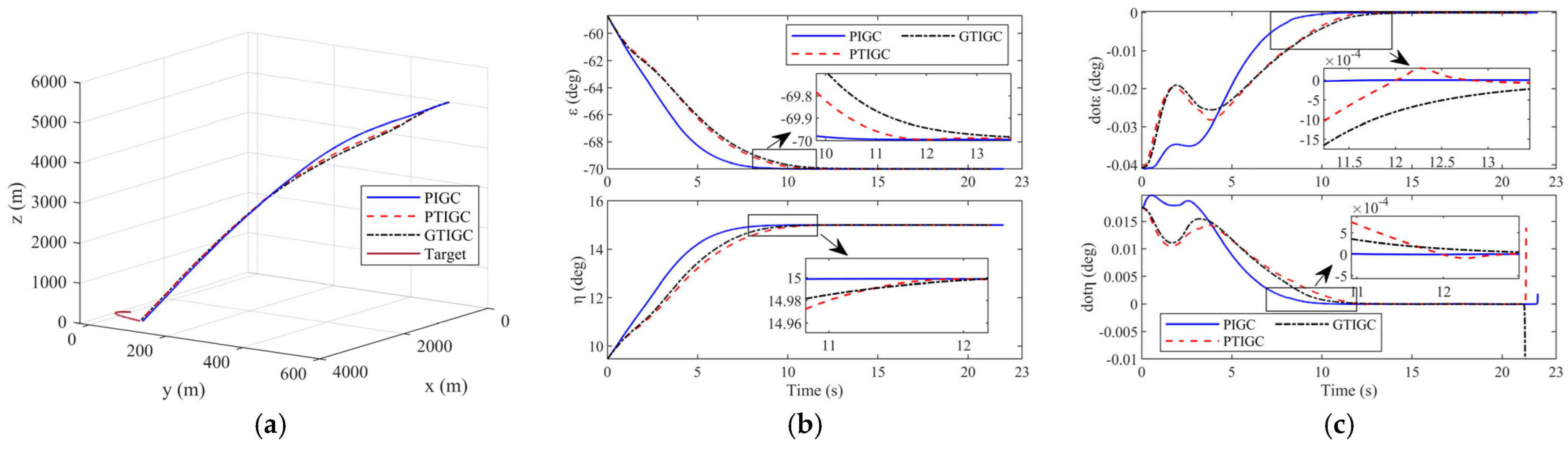
Figure 3a presents the trajectory comparison among PIGC, PTIGC, and GTIGC methods, all of which successfully hit the moving target. Figure 3b and depict the LOS angle and its rate. For PIGC, the LOS angle converges to the desired angle and the rate to zero within the prescribed time of 12 s, whereas GTIGC and GTFIGC converge to the desired angle at approximately 14 s. For both PIGC and PTIGC, the LOS angle converges to the desired value within the prescribed 12 s. However, PIGC exhibits a faster convergence rate. As shown in Figure 3c, the LOS angle rate of PIGC has already converged to zero at 11 s, whereas PTIGC still exhibits a slight overshoot at 12 s. In contrast, GTIGC has the slowest convergence rate, reaching the desired LOS angle at approximately 13 s. This demonstrates that the prescribed-time convergent sliding mode control can achieve a precise convergence time rather than just a bounded convergence time as in fixed-time control. Table 9 shows that the PIGC has the smallest miss distance.

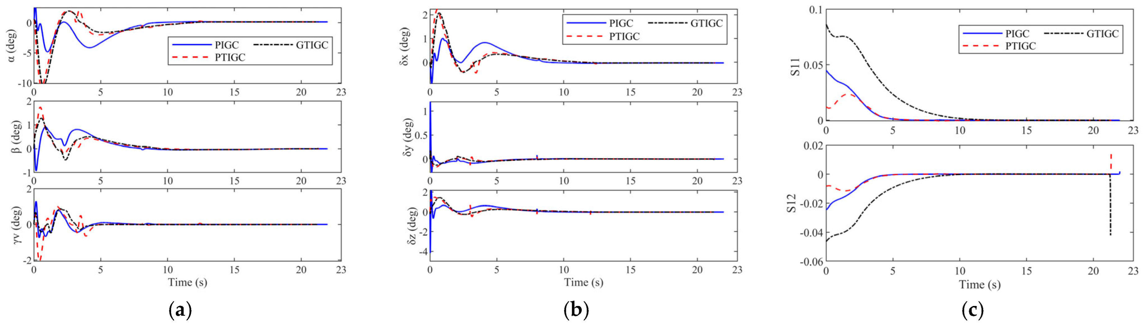
Figure 4a shows the variations in the attack angle, sideslip angle, and velocity roll angle. The convergence of these angles in PIGC is faster than in PTIGC and GTIGC. Figure 4b presents the aileron, rudder, and elevator deflections. Due to the large gain introduced by the time-varying function, PTIGC produces abrupt changes in the actuator command, resulting in small command jumps at approximately 3 s, 8 s, and 12 s. In contrast, PIGC employs a smoother time-varying function, leading to significantly smaller command variations than those of PTIGC.

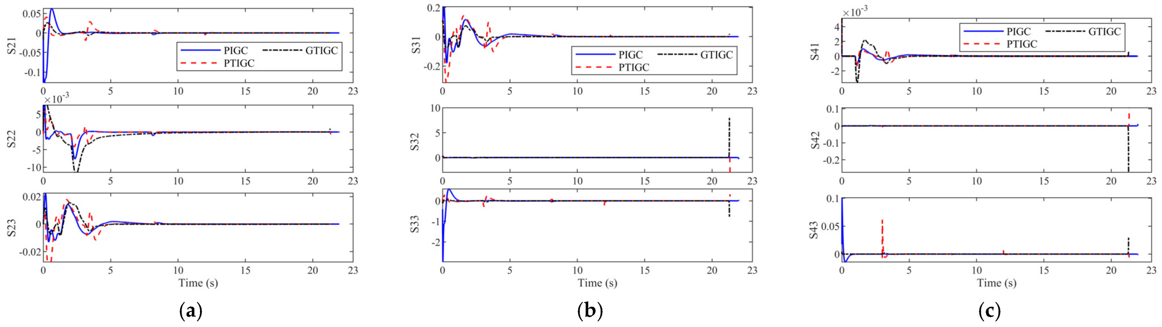
Figure 4c shows the evolution of the sliding surface ${\mathit{S}}_1$. With the prescribed-time convergent reaching law, PIGC and PTIGC ensures that ${\mathit{S}}_1$ converges to zero within 8 s, exhibiting faster convergence than the fixed-time GTIGC method. Figure 5a–c presents the variations in the sliding surfaces ${\mathit{S}}_2$, ${\mathit{S}}_3$, and ${\mathit{S}}_4$, all of which converge to zero within 8 s in PIGC and demonstrate rapid convergence.

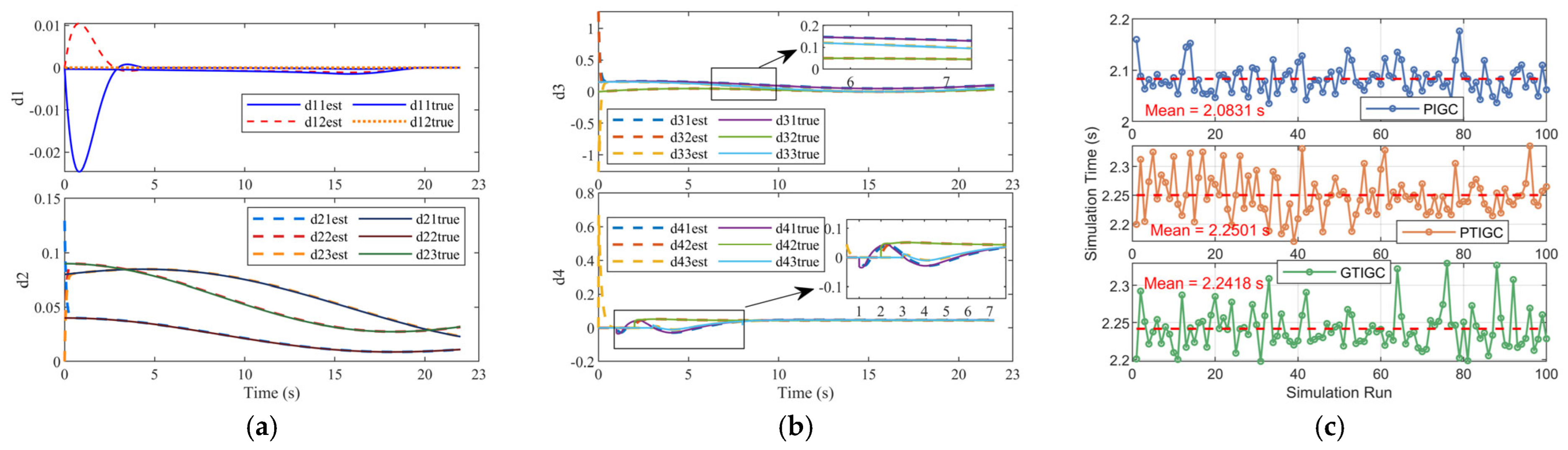
Finaly, Figure 6a compares the estimation results of the PtDO with the target acceleration disturbance ${\mathit{d}}_1$ and the airflow angle disturbance ${\mathit{d}}_2$. Figure 6b compares the estimation results of the PtDO with the angular velocity disturbance ${\mathit{d}}_3$ and the actuator fault disturbance ${\mathit{d}}_4$. The observer fully tracks the true disturbance within 5 s, indicating the effectiveness of the prescribed-time convergent disturbance observer. Figure 6c compares the computational time of the three methods over 100 simulation runs. PIGC, PTIGC, and GTIGC require average computational times of 2.0831 s, 2.2250 s, and 2.2418 s per run, respectively. Therefore, PIGC has the lowest computational cost among the three methods.

4.3. Simulation with Sensor Measurement Noise and Observer-Based State-Estimation Errors

Assumption 2 states that all vehicle states are available; however, the effects of sensor noise and state-estimation errors on the proposed control method should also be considered. Therefore, high-frequency sensor noise with an amplitude of ${0.1}^{°}$ for the airflow angle and $1^{°}$ for the angular rate is introduced, with frequencies of 30, 50, 70, and 90 Hz. In addition, state observation errors with amplitudes of $1 \mathrm{m}/\mathrm{s}$ for velocity and 5 m for position are considered. PIGC no noise corresponds to the noise-free simulation condition in Section 4.2, whereas PIGC noise further incorporates sensor noise and state-estimation errors based on Assumption 2. For actuator faults, $h_x,h_y,h_z=0.6$ and ${\upsilon }_x,{\upsilon }_y,{\upsilon }_z={0.6}^{\circ }$ are considered to further evaluate the robustness of the proposed method under more severe actuator fault conditions.

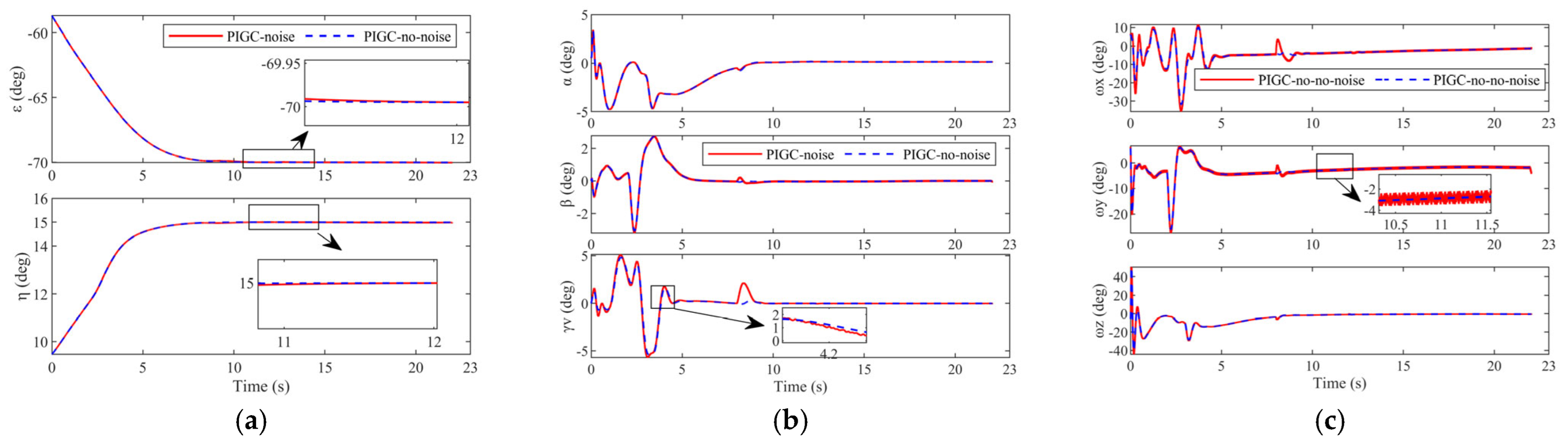
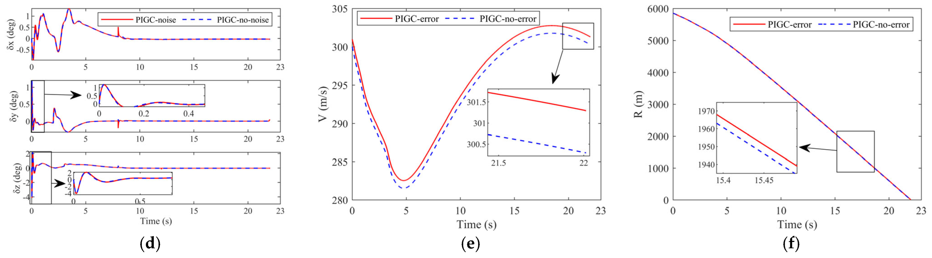
The simulation results are presented in Figure 7a–f and

Table 12. Simulation results for Case 2.

Case2	Arrival Time (s)	$\mathit{\epsilon }(\circ )$	$\mathit{\eta }(\circ )$	Miss Distance (m)
PIGC_no_noise	22.043	−70.009	15.007	0.179
PIGC_noise	22.041	−70.019	15.013	0.046

. Even in the presence of high-frequency measurement noise and state-estimation errors, together with more severe actuator faults, the proposed method can still successfully accomplish the task. The terminal errors remain below ${0.1}^{\circ }$ and converge to the desired values within the prescribed time of 12 s. Meanwhile, a small miss distance is maintained, and the arrival times remain close to the prescribed value. These results demonstrate the robustness of the proposed method against measurement noise, state-estimation errors, and severe actuator faults.

4.4. Cooperative Approach of Three Vehicles to a Moving Target with Different Desired Terminal Angles

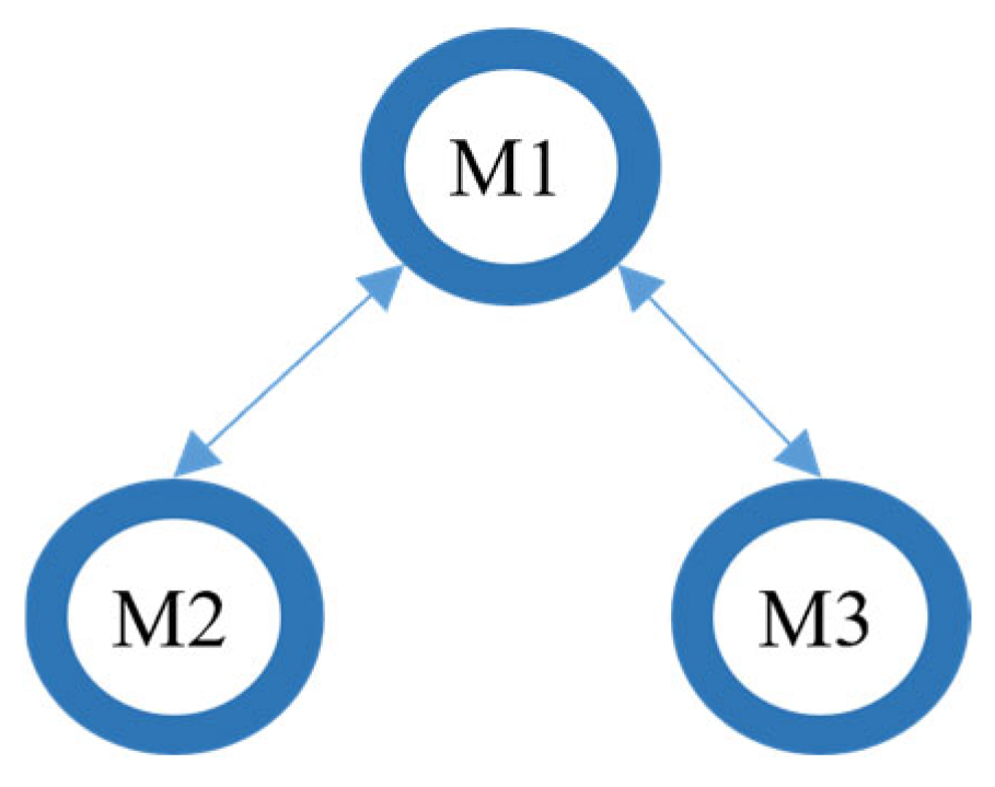
The communication topology of the three vehicles is shown in Figure 8, from which the communication matrix is $\mathit{C}=\left[\begin{array}{ccc}0& 1& 1\\ 1& 0& 0\\ 1& 0& 0\end{array}\right]$. The desired LOS elevation angle and LOS azimuth angle are set to ${\epsilon }_{d1}=-{70}^{\circ }$ and ${\eta }_{d1}={15}^{\circ }$ for Vehicle 1; ${\epsilon }_{d2}=-{70}^{\circ }$ and ${\eta }_{d2}={20}^{\circ }$ for Vehicle 2; ${\epsilon }_{d3}=-{65}^{\circ }$ and ${\eta }_{d3}={10}^{\circ }$ for Vehicle 3. The cooperative guidance law and prescribed arrival time depend on the vehicles’ initial positions and velocities, as well as their aerodynamic drag and available thrust. Higher thrust and lower drag allow a wider feasible range of initial conditions while maintaining the prescribed arrival time.

To verify the effectiveness of the proposed method, two comparative studies are conducted with the proposed PCIGC scheme. In Case 1 (PTCIGC and GTCIGC), the GTCIGC and PTCIGC methods are combined with the cooperative guidance law proposed in this paper, which is used to compare the convergence speed of the LOS angles, as well as the variation curves of airflow angles and actuator deflections. In Case 2 (PCIGC-Slow), the cooperative guidance law proposed in [37] is adopted, which is used to compare the convergence speed of the remaining flight time of the three vehicles.

$$\left\{\begin{array}{l}{u}_{ri}={\displaystyle \frac{x_{2i}^2}{x_{1i}}}\left\{{\displaystyle \frac{x_{1i}^2{x}_{4i}^2}{x_{2i}^2}}+{\displaystyle \frac{x_{1i}^2{\dot{\eta }}_i^2{\cos }^2{\epsilon }_i}{x_{2i}^2}}+{\delta }_{ri}sat\left(t_{ai}-t_a^{\ast }\right)-{\alpha }_1{\displaystyle \sum _{j\in {\mathcal{N}}_i}{c}_{ij}}{\left(t_{goj}-t_{goi}\right)}^{q_1}-{\alpha }_3{\displaystyle \sum _{j\in {\mathcal{N}}_i}{c}_{ij}}{\left(t_{goj}-t_{goi}\right)}^{p_1}\right\}\\ {\dot{\delta }}_{ri}={\chi }_1\left|t_{ai}-t_a^{\ast }\right|\end{array}\right.$$

(60)

where ${\alpha }_1=0.001$, ${\alpha }_3=0.001$, ${\chi }_1=0.05$, $t_a^{\ast }=18s$, $q_1=1.286$, $p_1=0.714$.

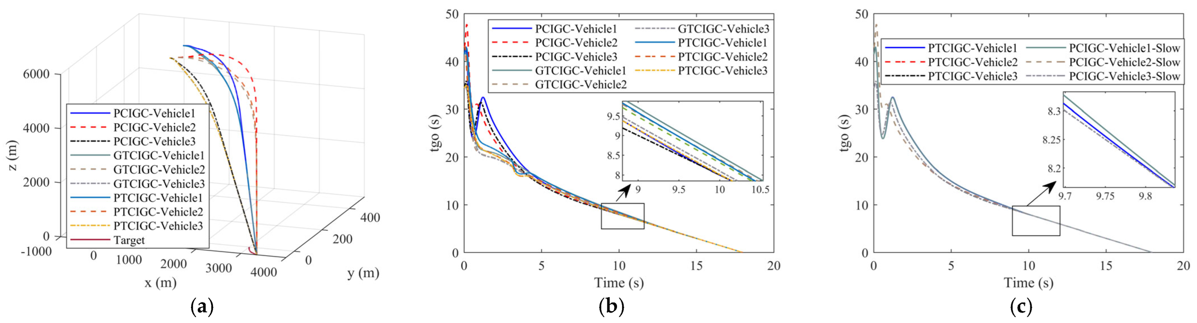
The trajectory curves of the three vehicles in cooperative arrival are shown in Figure 9a. The vehicles are launched from different positions to approach a moving target at specified terminal angles. Figure 9b represents the comparison of the remaining flight time for PCIGC, PTCIGC and GTCIGC. Both methods achieve target interception at $t=17.98 s$; moreover, the remaining flight times of the three vehicles under PCIGC converge to consensus more rapidly. Figure 9c illustrates a comparison between the PCIGC using the proposed cooperative guidance law and the PCIGC-Slow using the conventional method. As shown in the Figure 9c, the improved guidance law enables the remaining flight times of the three vehicles to reach consensus more rapidly.

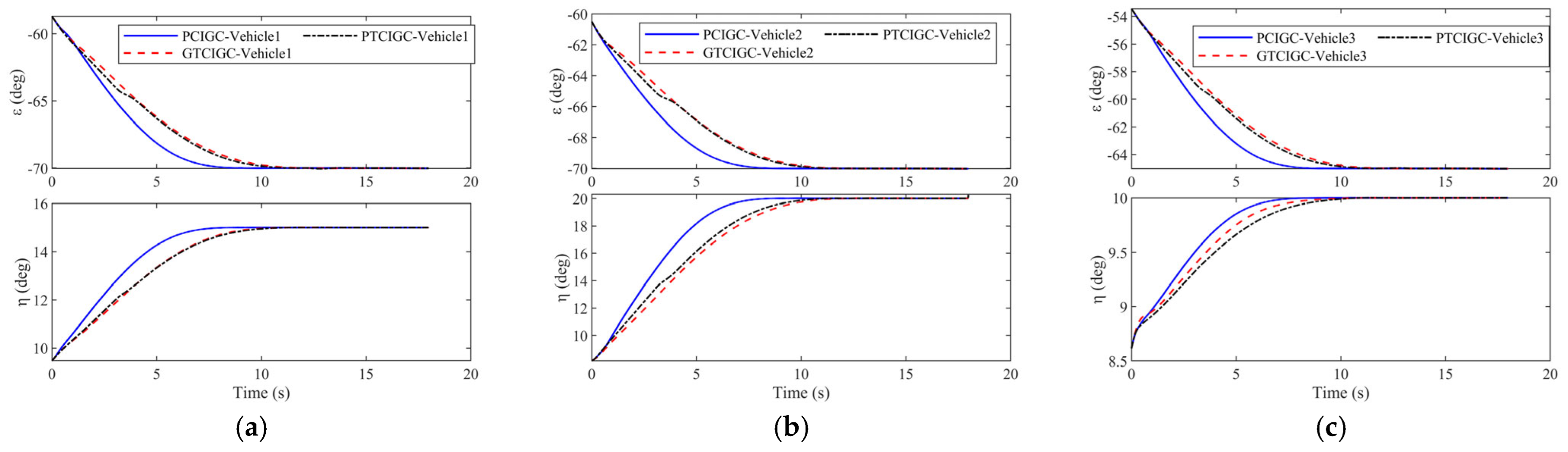
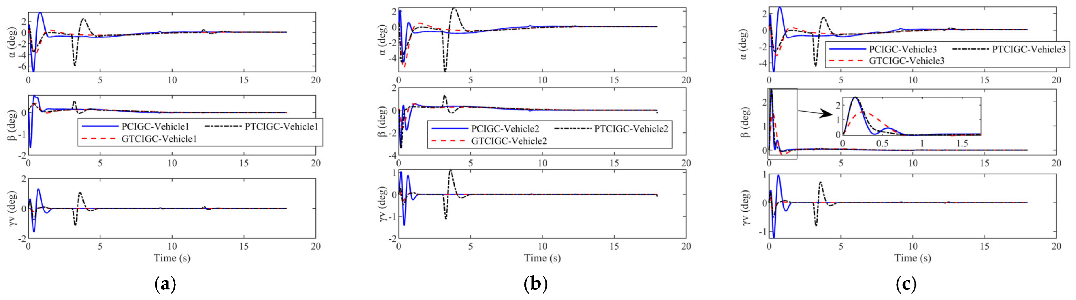
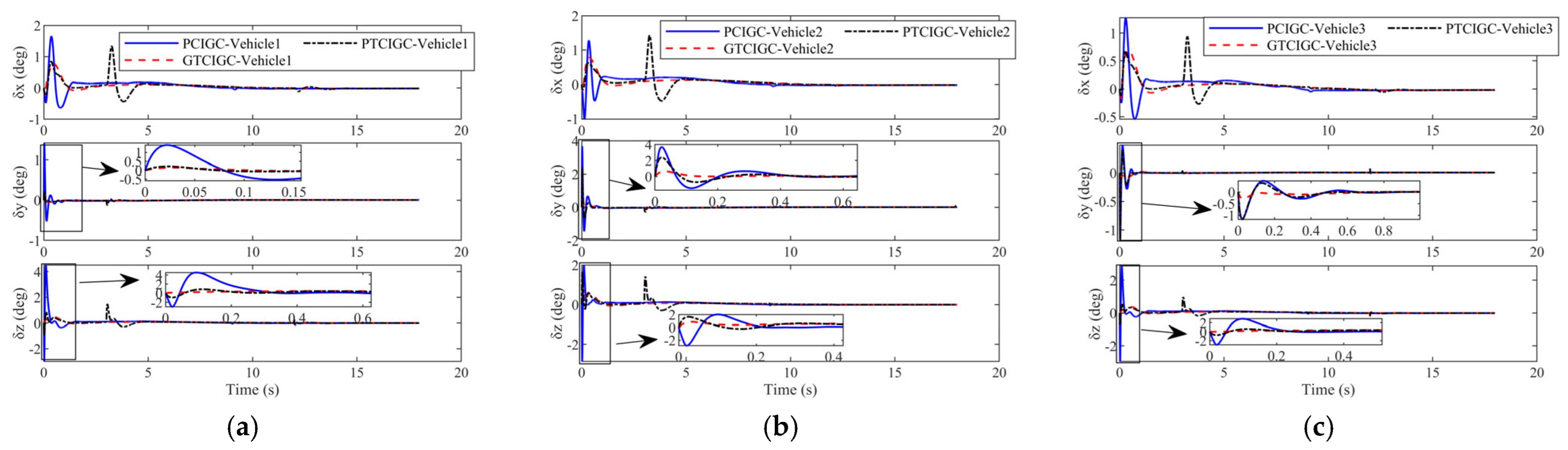
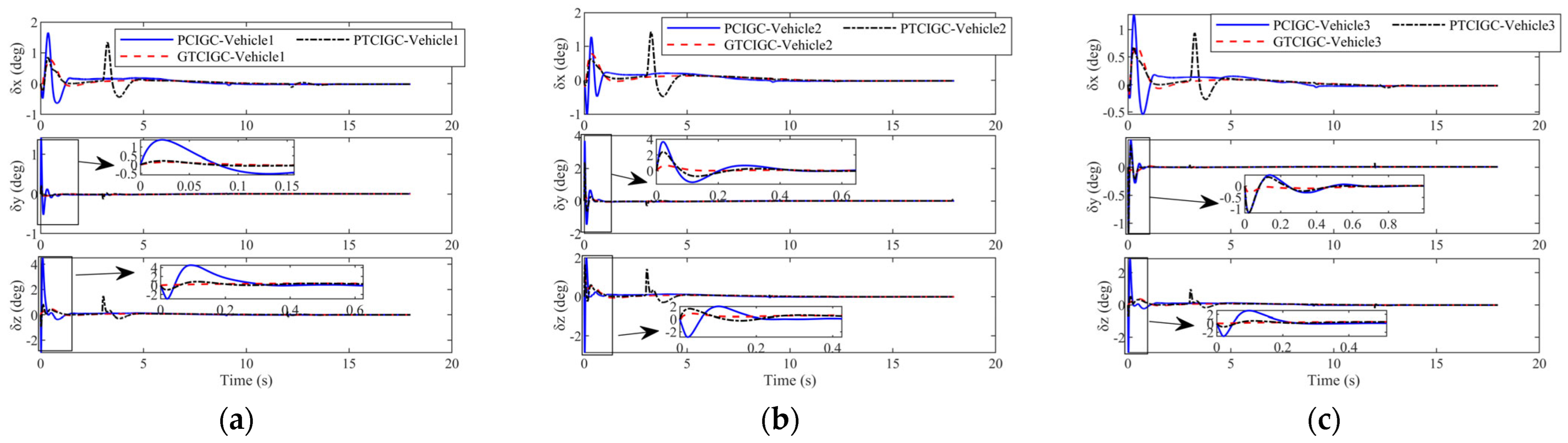
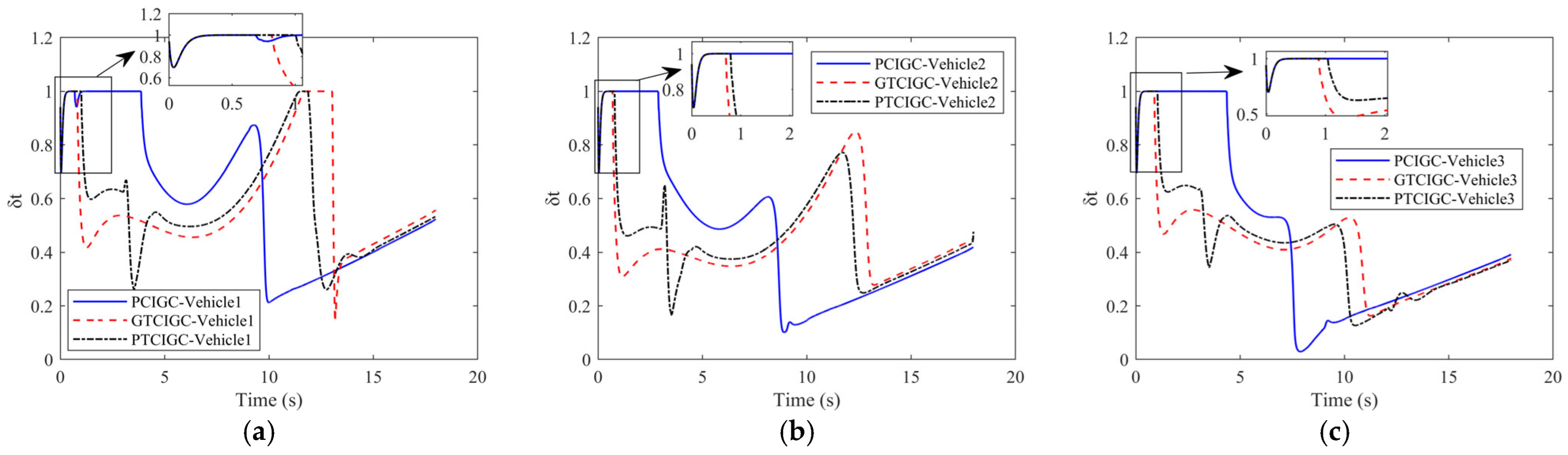
Figure 10a–c illustrates the LOS angle variations in vehicles 1, 2, and 3, respectively. The results indicate that PCIGC ensures convergence to the desired values within the prescribed time of 12 s, which is faster than that of PTCIGC and GTCIGC. Figure 11a–c represents the airflow angle variations in vehicles 1, 2, and 3, respectively, which eventually converge to zero. Figure 12a–c represents the actuator deflection responses of vehicles 1, 2, and 3. Despite the presence of actuator faults, the system maintains normal operation under the compensation of the disturbance observer.

Table 13. Simulation results for Case 3.

Case 3	Arrival Time (s)	$\mathit{\epsilon }(\circ )$	$\mathit{\eta }(\circ )$	Miss Distance (m)
PCIGC-Vehicle1	17.983	−70.014	15.009	0.257
PTCIGC-Vehicle1	17.983	−70.009	15.008	0.286
GTCIGC- Vehicle1	17.983	−70.007	14.998	0.337
PCIGC-Vehicle2	17.983	−70.014	19.996	0.002
PTCIGC-Vehicle2	17.983	−70.013	20.300	0.044
GTCIGC- Vehicle 2	17.983	−70.008	19.995	0.078
PCIGC-Vehicle 3	17.983	−65.020	9.999	0.180
PTCIGC-Vehicle 3	17.983	−65.014	9.999	0.234
GTCIGC- Vehicle 3	17.983	−65.012	9.999	0.222

presents the simulation results of miss distance, line-of-sight angle error, and arrival-time parameters.

Figure 13a–c depicts the thrust commands of vehicles 1, 2, and 3, respectively. Figure 14a–c illustrates the corresponding velocity tracking responses.

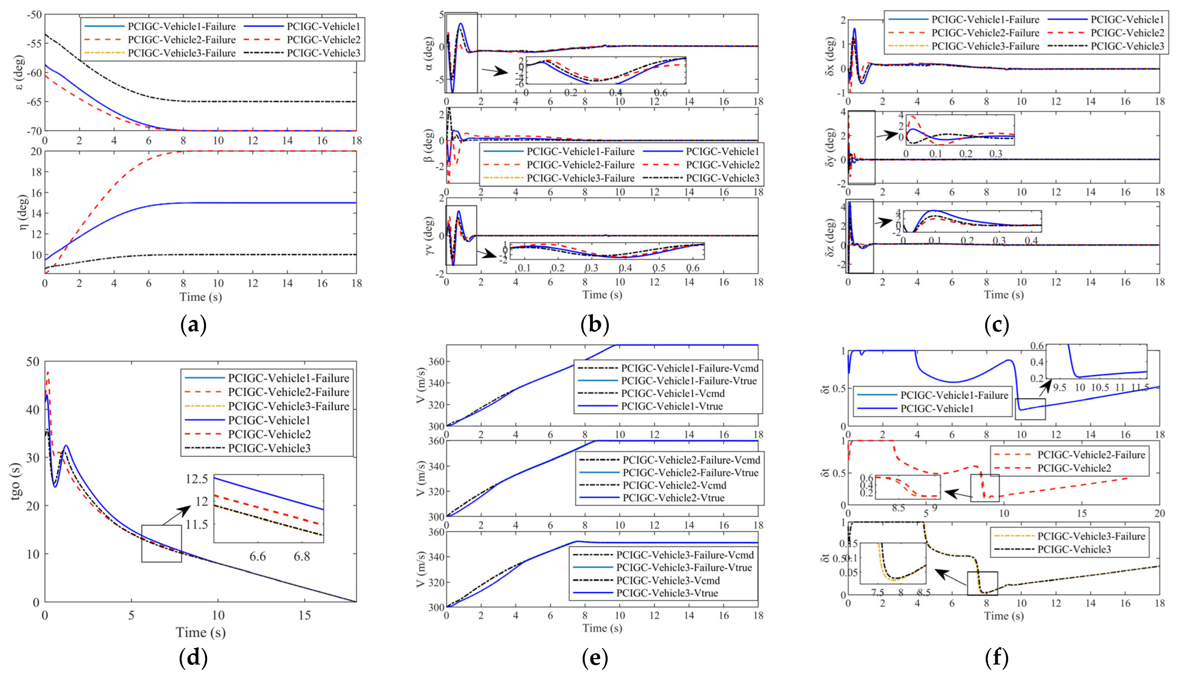
4.5. Cooperative Approach of Three Vehicles Under Communication Failure

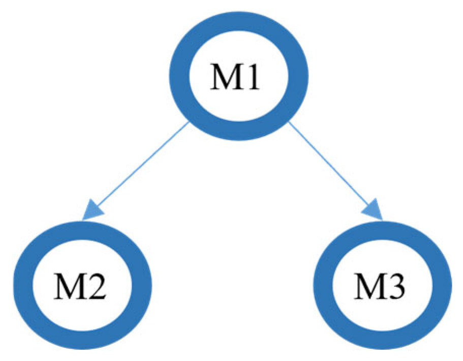
The faulty communication topology of the three vehicles is shown in Figure 15, from which the communication matrix is $\mathit{C}=\left[\begin{array}{ccc}0& 1& 1\\ 0& 0& 0\\ 0& 0& 0\end{array}\right]$. PCIGC is compared to its communication failure counterpart, denoted as PCIGC-Failure. The flight conditions and controller parameter settings are the same as those used in Section 4.4.

The simulation results are presented in Figure 16a–f and

Table 14. Simulation results for Case 4.

Case4	Arrival Time (s)	$\mathit{\epsilon }(\circ )$	$\mathit{\eta }(\circ )$	Miss Distance (m)
PCIGC-Vehicle1	17.983	−70.014	15.009	0.257
PCIGC-Vehicle1-Failure	17.983	−70.014	15.009	0.256
PCIGC-Vehicle2	17.983	−70.014	19.996	0.002
PCIGC-Vehicle2-Failure	17.983	−70.014	19.996	0.005
PCIGC-Vehicle3	17.983	−65.020	9.999	0.180
PCIGC-Vehicle3-Failure	17.983	−65.020	9.999	0.181

. Although the communication topology is degraded to one-way communication due to the communication failure, the cooperative guidance law does not affect the IGC performance of the three vehicles. The remaining flight times still converge to consensus, and the velocity tracking performance remains essentially unchanged. These results demonstrate that the proposed algorithm maintains satisfactory cooperative engagement performance and possesses strong tolerance to communication failures.

4.6. Monte Carlo Validation of Cooperative Multi-Vehicle

The aerodynamic parameters of each vehicle are randomly perturbed within $\pm 20\%$ uniform distribution around their nominal values. Vehicles 1–3 are randomly released within circular regions of radius 100 m centred at (0 m, 5000 m, 500 m), (0 m, 5000 m, 0 m), and (0 m, 5000 m, −500 m), respectively, with their desired LOS elevation angle and LOS azimuth angle constrained within the ranges of ${\epsilon }_{d1}=(-{65}^{\circ },-{70}^{\circ })$ and ${\eta }_{d1}=({15}^{\circ },{20}^{\circ })$, ${\epsilon }_{d2}=(-{65}^{\circ },-{70}^{\circ })$ and ${\eta }_{d2}=(-5^{\circ },5^{\circ })$, ${\epsilon }_{d3}=(-{65}^{\circ },-{70}^{\circ })$ and ${\eta }_{d3}=(-{15}^{\circ },-{20}^{\circ })$, respectively. 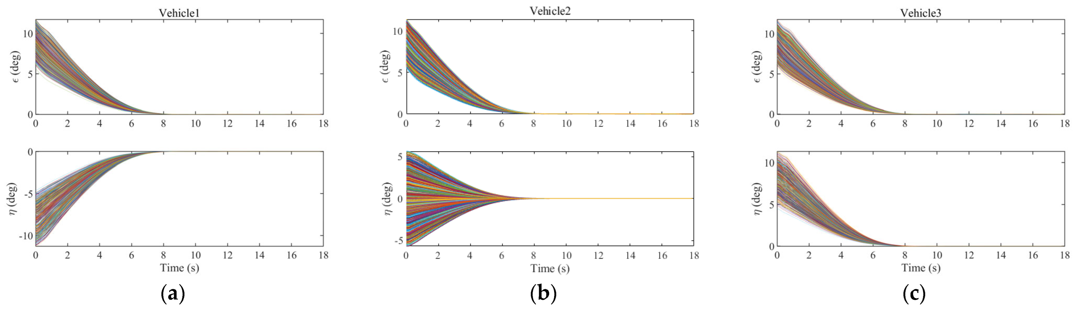The remaining parameters are identical to those in Section 4.1. A total of 500 Monte Carlo simulations are performed. The simulation results are shown in Figure 17 and Figure 18.

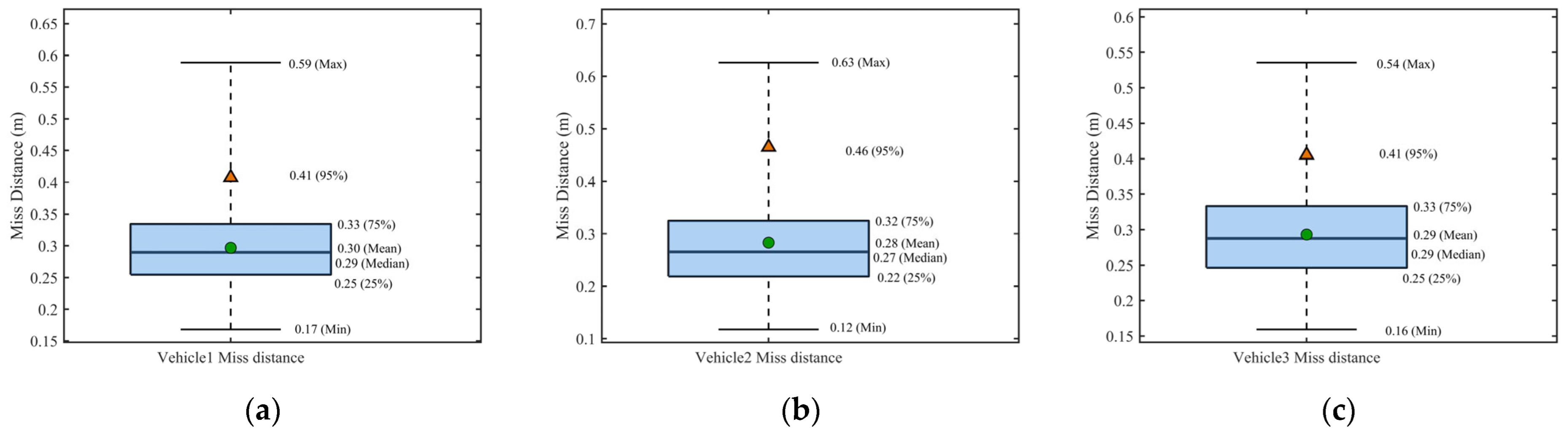
As shown in the box plots in Figure 17, the miss distances of all three vehicles remain below 1 m throughout the 500 Monte Carlo simulations, with mean miss distances of approximately 0.3 m. For Vehicle 1, the mean, standard deviation, minimum, maximum, and 95th percentile of the miss distance are 0.2967 m, 0.0648 m, 0.1684 m, 0.5887 m, and 0.4077 m, respectively. For Vehicle 2, the corresponding values are 0.2830 m, 0.0923 m, 0.1178 m, 0.6263 m, and 0.4650 m, respectively. For Vehicle 3, the corresponding values are 0.2931 m, 0.0644 m, 0.1594 m, 0.5357 m, and 0.4052 m, respectively. As indicated by the box plots, the miss distance data exhibit compact distributions with relatively narrow interquartile ranges and no pronounced dispersion, which is also consistent with the small standard deviations. No failure is observed for any of the three vehicles, resulting in a failure probability of 0.00%. These results demonstrate that the proposed algorithm maintains high accuracy and stability, while exhibiting strong robustness against aerodynamic parameter uncertainties. Blue areas represent the parameter distribution ranging from 20% to 75%. Green circles denote the positions of the mean values, and orange triangles represent the 95% parameter distribution.

As shown in Figure 18, the LOS angle error of each vehicle converges to the desired value within the prescribed time of 12 s, demonstrating the prescribed-time convergence performance of the proposed algorithm.

5. Conclusions

This paper addresses fast convergence, actuator faults, external disturbances, velocity control, and communication constraints in cooperative multi-vehicle tasks. A cooperative integrated guidance and control (CIGC) method for three vehicles is proposed based on a “single-vehicle-first, cooperative-later” strategy.

For single-vehicle control, prescribed-time sliding mode control, dynamic surface control, a prescribed-time disturbance observer, and a compensated nonlinear filter are integrated with line-of-sight (LOS) angle constraints. The proposed method achieves fast and accurate tracking under actuator faults and external disturbances. Simulation results show that the LOS angle errors converge within 12 s, with faster convergence than fixed-time and conventional prescribed-time methods. Even in the presence of measurement noise and state-estimation errors, the proposed control method can still accomplish the task.

For multi-vehicle coordination, a velocity controller is introduced to regulate speed through thrust control, and a prescribed-time cooperative law is designed to synchronize the time-to-go of the three vehicles. The vehicles achieve coordinated arrival at the prescribed 18 s time. Compared to fixed-time methods, the proposed approach provides direct convergence-time specification with a simpler design.

Under communication faults and aerodynamic uncertainties, the method maintains good cooperative performance with one-way communication. In 500 Monte Carlo simulations, the miss distance remains below 1 m, while the LOS angle errors converge to 0° within 12 s, demonstrating the robustness of the proposed method.

The method is currently validated through model-in-the-loop simulations. Future work will focus on hardware-in-the-loop and real-time testing to further evaluate its effectiveness and engineering applicability.