Koopman Predictor-Based Integrated Guidance and Control Under Multi-Force Compound Control System

Abstract

This paper proposes a Koopman-predictor-based integrated guidance and control (IGC) law for the hypersonic target interceptor under the multi-force compound control. The strongly coupled and nonlinear guidance and control systems including the characteristics of the aerodynamic rudder, attitude control engine and orbit control engine are described as a linear IGC model based on the Koopman predictor. The proposed IGC law adapted to the linear IGC model is presented by combining the sliding mode control (SMC), the extended disturbance observer (EDO), and the adaptive weight-based control allocation scheme for being robust against the uncertainties and optimizing the fuel allocation for the fuel limited interceptor while intercepting the targets precisely. The stability of the proposed control law-based closed-loop system is guaranteed. The effectiveness and robustness of the proposed control law are proved by simulation comparisons and Monte Carlo tests.

1. Introduction

The large vertical altitude span and unpredictable flight path of hypersonic vehicles pose great challenges to interception missions [1,2]. The existing hypersonic target interceptors adopt a compound control system consisting of the aerodynamic rudder, attitude control engine and orbit control engine, focusing on the interception in specific atmospheric environments [3,4,5,6]. The compound control system composed of the aerodynamic rudder/attitude control engine and aerodynamic rudder/orbit control engine are suitable for interception in a dense atmospheric environment, while the compound control system composed of the attitude control engine/orbit control engine is suitable for interception in a thin or vacuum atmospheric environment.

However, the evolution of advanced hypersonic targets with their growing maneuvering capability requires the interceptors to operate seamlessly within and between the boundaries of low endo-, high endo-, and exoatmospheric regimes [7]. The control efficiency of the aerodynamic rudder decreases with the decrease in atmospheric density. The attitude and orbit control engines generate the attitude and divert thrusts, respectively, and they are necessary for maintaining the ability to control the attitude and trajectory in a thin or vacuum atmospheric environment. The use of attitude and orbit control engines consumes fuel, but carrying too much fuel increases the weight of the interceptor, thus reducing its flight speed. The denser the atmosphere, the greater the thrust required for the engine to generate the required acceleration, and the greater the fuel consumption. Considering the shortcomings of the aerodynamic rudder, attitude and orbit control engines mentioned above, the existing compound control schemes consisting of two different actuators are not suitable for wide-airspace interception missions and struggle to cope with advanced hypersonic targets with the ability to fly across the low endo-, high endo-, and exoatmospheric regimes. Therefore, the multi-force compound control system composed of an aerodynamic rudder, attitude control engine, and orbit control engine is the future development trend.

There are significant differences in the working principles of the aerodynamic rudder, attitude control engine, and orbit control engine, as well as their impact on interceptors. The aerodynamic rudder adjusts the attitude of the interceptor and controls the trajectory by generating moment increments, the control performance of which decreases dramatically with decreasing the atmospheric density. The attitude control engine has complex functions. In a dense atmospheric environment, it generates moment increments through the thrust to control the attitude and trajectory; in a thin or vacuum atmospheric environment, it can only be used to adjust the attitude but cannot realize the effective impact on the trajectory. The orbit control engine is applied for interceptor trajectory control by generating the thrust to change the acceleration, and its control efficiency improves with decreasing atmospheric density. However, with the fuel consumption of engines, the drift of the mass center is inevitable, leading to significant additional moment increments to interfere with the attitude control. The above issues result in strong couplings for the interceptor under the multi-force compound control. The existing research works on interceptors under the compound control mainly reduce the complexity of the model through decoupling, thereby simplifying the design of the controller, and they do not consider the coupling effects completely or partially in the controller design. Refs. [4,5] treated the attitude control engine as a compensation for the aerodynamic rudder, considering that the attitude thrust produces only moment increments, ignoring its direct effect on the acceleration. Refs. [6,7,8] designed the guidance and the control systems as the outer and inner loops, respectively, where the effect of the attitude control engine on the trajectory is taken into account but the effect of the orbit control engine on the attitude is ignored.

Traditionally, the guidance and control systems of aerospace vehicles are designed independently as the outer and inner loops. The guidance commands are transmitted unidirectionally from the outer loop to the inner loop, so it is impossible to introduce complex couplings between the guidance/control systems in the controller design. The integrated guidance and control (IGC) considering the outer and inner loops as a whole is proposed as an improvement. The IGC faces the challenge of high relative order from the control input to the output, so most existing IGC laws are designed by combining the backstepping control with the robust control [9,10,11,12,13]. However, the essence of backstepping control is to decouple the high-order system into several independent first-order subsystems, and connect theses subsystems through virtual control inputs, which cannot be used for the high-order system with strong couplings. In a few existing studies, control methods for high-order systems such as adaptive dynamic programming [14] and high-order sliding mode control [15,16,17] have been used to avoid the occurrence of decoupling and virtual control inputs. On the basis of these high-order control methods, [18,19] proposed the IGC laws for strongly coupled guidance and control systems under compound control, introducing coupling effects into the controller design to improve the performance. However, these studies utilized/compensated for the effects caused by couplings at the cost of increasing the complexity of the control design.

The Koopman operator proposed by [20] is an inherently data-driven operator, discovering the suitable coordinates to describe the nonlinear systems by the globally linear models. Koopman operators are widely used for the prediction, analysis, and control of complex nonlinear systems, transforming higher-order, nonlinear systems into first-order linear systems by increasing the model dimensions, enabling researchers to flexibly apply more efficient and advanced control techniques to nonlinear systems [21,22,23,24,25]. For the high-speed missiles under aerodynamic rudder control, [26] used the Koopman operator to establish a linear model and designed the IGC law based on the model predictive control. However, to the best of our knowledge, the existing research on IGC lacks the attention and application of Koopman operator theory, especially for the IGC system under multi-force compound control with high-order, strong coupling, and strong nonlinearity.

Therefore, this paper studies the IGC law for the hypersonic target interceptor subjected to the complex dynamics of the aerodynamic rudder, attitude control engine, and orbit control engine. The main contributions are summarized as follows.

(1)

The mathematical model of the strapdown interceptor under the multi-force compound control is established, taking into account the physical limitations, working principles, and dynamic characteristics of the aerodynamic rudder, attitude control engine, and orbit control engine.

(2)

The high-order, strongly coupled, and strongly nonlinear interceptor kinematics/dynamics model under multi-force compound control is transformed into a linear IGC model using the Koopman predictor on the premise of satisfying the accuracy.

(3)

Based on the linear IGC model, the extended disturbance observer (EDO) and adaptive weight-based control allocation scheme are combined with the Koopman predictor-based sliding mode control (KPSMC) to form the IGC law for the interceptor under the multi-force compound control. The proposed Koopman predictor-based IGC method simplifies the complex model while retaining the dynamic characteristics, balancing the difficulty of the controller design and the control performance.

The content of this paper is arranged as follows. The mathematical model of the multi-force compound control system and strapdown interceptor are listed in Section 2. The IGC model based on the Koopman operator is constructed in Section 3. The Koopman predictor-based IGC law and allocation law are designed in Section 4. Simulation studies are demonstrated in Section 5. Finally, Section 6 concludes this paper.

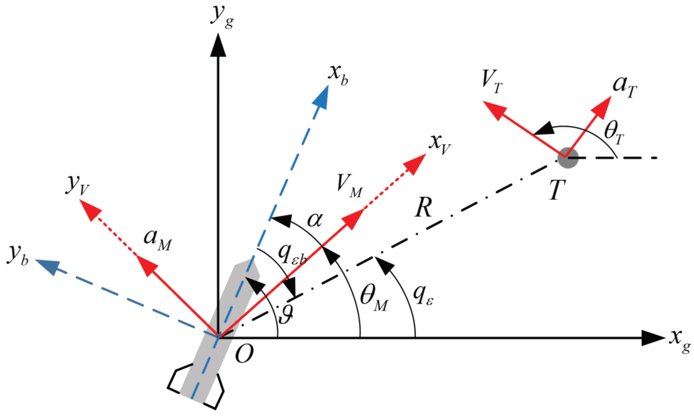
2. Problem Formulation

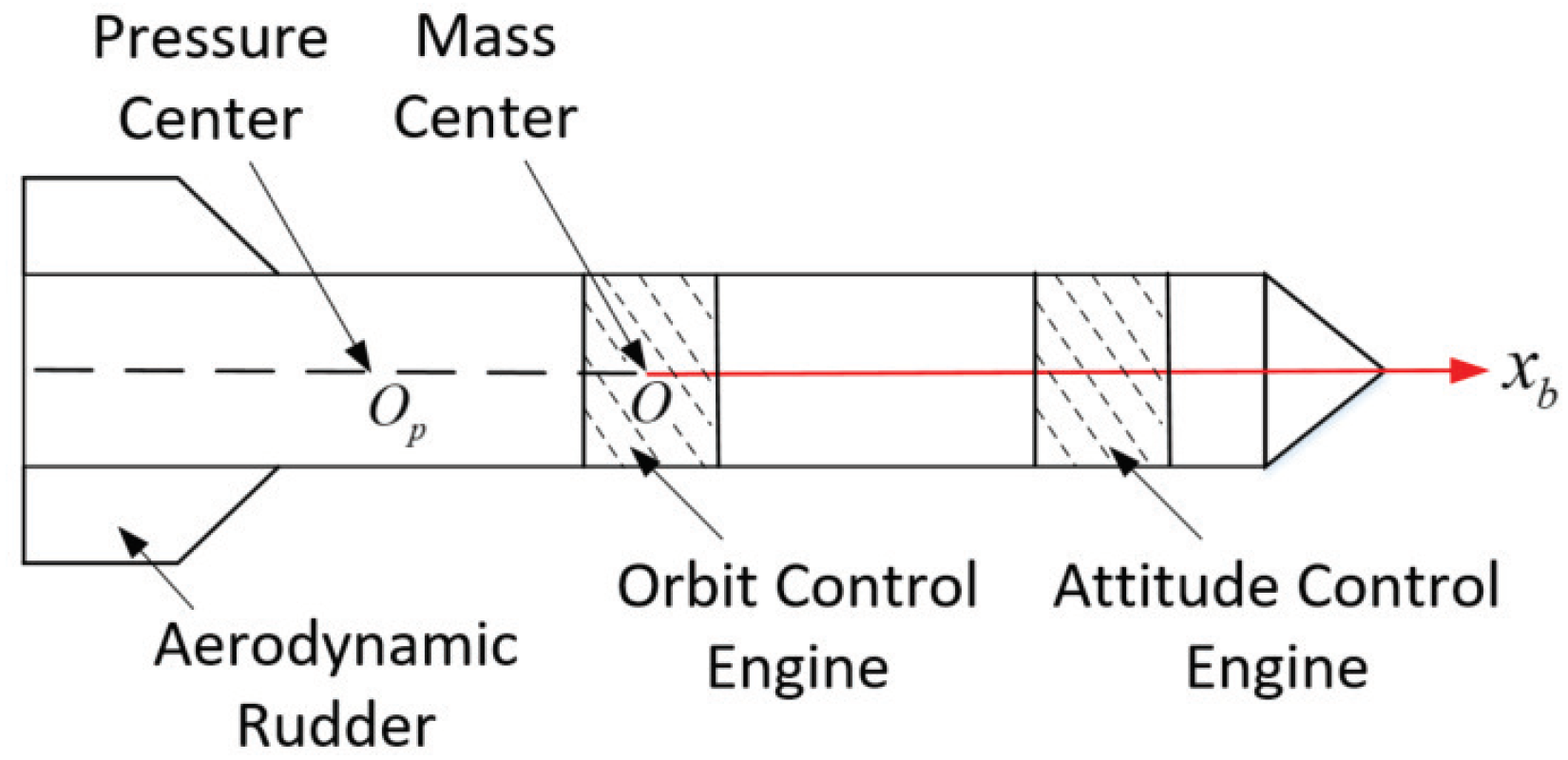
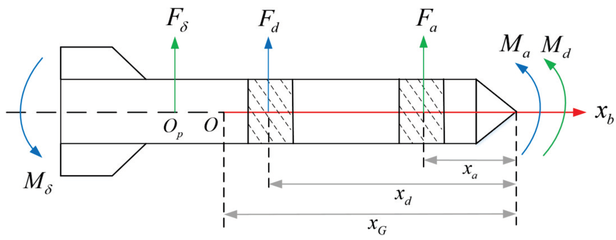
2.1. Multi-Force Compound Control System

The multi-force compound control system, consisting of the aerodynamic rudder, attitude control engine, and orbit control engine, is proposed for intercepting high-speed targets over a wide airspace. Generally, the mounting positions of the actuators are shown in Figure 1, where O is the mass center, $O_p$ is the pressure center, and $O{x}_b$ is the interceptor body axis. The aerodynamic rudder is mounted on the tail of the interceptor, generating moment increment by adjusting the deflection angle. The attitude control engine is mounted at a distance from the mass center of the interceptor, generating moment increment by providing the attitude thrust. The orbit control engine is mounted at the mass center of the interceptor, generating acceleration increment by providing the divert thrust. The thrust provided by the orbit control engine and attitude control engine is perpendicular to the body axis of the interceptor. Generally, the thrust of the orbit control engine is much larger than that of the attitude control engine.

The desired effects of the actuators are shown in Figure 2, where the aerodynamic rudder and the attitude control engine only generate the moment increment $M_{\delta }$ and $M_a$, respectively, and the orbit control engine only generates the force increment $F_d$. However, the following complex effects exist in the actual multi-force compound control system:

(1)

The aerodynamic rudder and attitude control engine inevitably generate the force increments while generating the moment increments that affect the trajectory. Among them, the additional acceleration increment generated by the attitude control engine is particularly significant.

(2)

Due to the drift of the mass center caused by installation error and fuel consumption, the action point of the divert thrust is unavoidably deviated from the mass center, resulting in additional moment disturbance to the attitude.

(3)

The thrusts provided by the engines are fixedly connected to the interceptor.

According to the above issues, although the functions and working principles of each actuator are different, they can all generate moment and force increments simultaneously, leading to strong control inputs coupling. The actual effects of the multi-force compound control system are shown in Figure 3, where the blue and green arrows represent the desired and additional force/moment increments, respectively. $M_d$ is the additional moment increment of the orbit control engine, and $F_a$ and $F_{\delta }$ are the additional force increments of the attitude control engine and the aerodynamic rudder, respectively.

Taking the longitudinal plane as an example and considering the control inputs coupling, the force and moment models of interceptor under the multi-force compound control can be described as follows:

$$\begin{array}{cc}\hfill F=& qS{c}_y^{\alpha }\alpha +qS{c}_y^{\delta }\delta +F_{d}cos\alpha +F_{a}cos\alpha -mgcos{\theta }_M\hfill \\ \hfill M=& {\displaystyle \frac{qS{L}^2}{2V_M}}{m}_z^{{\omega }_z}{\omega }_z+qSL{m}_z^{\alpha }\alpha +qSL{m}_z^{\delta }\delta +F_d({\mathit{x}}_G-{\mathit{x}}_d)+F_a({\mathit{x}}_G-{\mathit{x}}_a)\hfill \end{array}$$

(1)

where F and M are the external force and moment on the interceptor, respectively. $F_d$, $F_a$, and $\delta$ are the divert thrust, the attitude thrust, and the deflection angle of the aerodynamic rudder. $q={\displaystyle \frac{1}{2}}\rho V_M^2$ is the dynamic pressure, where $\rho$ and $V_M$ are the air density and velocity of the interceptor, respectively. $\alpha$, ${\theta }_M$, and ${\omega }_z$ are the angle of attack, the flight path angle of the interceptor, and the angular pitch rate, respectively. $c_y^{\alpha }$ and $c_y^{\delta }$ are the lift force derivatives with respect to $\alpha$ and $\delta$, respectively. $m_z^{\alpha }$, $m_z^{{\omega }_z}$, and $m_z^{\delta }$ are the pitch moment derivatives with respect to $\alpha$, ${\omega }_z$, and $\delta$, respectively. S, L, m, and g are the aerodynamic reference area, the reference length, the mass of the interceptor, and the gravity acceleration, respectively. ${\mathit{x}}_G$ is the length from the mass center to the warhead. ${\mathit{x}}_d$ and ${\mathit{x}}_a$ are the lengths from the action point of the divert thrust and attitude thrust to the warhead, respectively.

In the multi-force compound control system, each actuator has different dynamic characteristics. The dynamics of attitude and divert thrusts can be written as the following first-order system:

$$\begin{array}{cc}\hfill & F_d={\displaystyle \frac{1}{{\tau }_{d}s+1}}{F}_{dc}\hfill \\ \hfill & F_a={\displaystyle \frac{1}{{\tau }_{a}s+1}}{F}_{ac}\hfill \end{array}$$

(2)

where $F_{dc}$ and $F_{ac}$ are the control commands for the divert thrust and attitude thrust, respectively. $F_d$ and $F_a$ are the actual divert thrust and attitude thrust acting on the controlled interceptor, respectively. ${\tau }_d$ and ${\tau }_a$ are the response delay parameters of the divert thrust and attitude thrust, respectively.

The dynamics of aerodynamic rudder can be written as the following second-order system:

$$\delta ={\displaystyle \frac{{\omega }_{\delta }^2}{s^2+2\xi {\omega }_{\delta }s+{\omega }_{\delta }^2}}{\delta }_c$$

(3)

where ${\delta }_c$ is the control command for the deflection angle of the rudder. $\delta$ is the actual deflection angle of the rudder. ${\omega }_{\delta }$ and $\xi$ are the natural frequency and damping ratio of the aerodynamic rudder, respectively.

The input saturations of the divert thrust, attitude thrust, and deflection angle yield the following:

$$\begin{array}{cc}\hfill \left|F_d\right|& \le F_{d max}\hfill \\ \hfill \left|F_a\right|& \le F_{a max}\hfill \\ \hfill \left|\delta \right|& \le {\delta }_{max}\hfill \end{array}$$

(4)

where $F_{d max}$, $F_{a max}$, and ${\delta }_{max}$ are the maximum values of the divert thrust, attitude thrust, and deflection angle, respectively.

The generation of deflection angle does not consume fuel, so there is no limitation to the total energy of the aerodynamic rudder control. In contrast, the generation of the divert thrust and attitude thrust is limited by the total fuel as follows:

$$\begin{array}{cc}\hfill & \left|I_d\right|\le I_{ds\mathit{U}m}\hfill \\ \hfill & \left|I_a\right|\le I_{as\mathit{U}m}\hfill \end{array}$$

(5)

where $I_d={\int }_0^t\left|F_d\right|dt$ and $I_a={\int }_0^t\left|F_a\right|dt$ are the impulse consumed by the orbit engine and attitude engine, respectively. $I_{dsum}$ and $I_{asum}$ are the total impulse that the orbit engine and attitude engine can provide, respectively.

2.2. Mathematical Model for Strapdown Interceptor Under Multi-Force Compound Control

The seeker of the strapdown interceptor is fixedly connected to the warhead, and the measurement information of it is the body line-of-sight (BLOS) angle [27,28,29]. Figure 4 is the strapdown interceptor–target engagement geometry in longitudinal plane, where O and T are the mass centers of the interceptor and target, respectively. $x_{g}O{y}_g$, $x_{V}O{y}_V$, and $x_{b}O{y}_b$ denote the ground coordinate system, the velocity coordinate system, and the body coordinate system, respectively. R, $q_{ϵ}$, and ${q_{ϵ}}_b$ represent the interceptor–target relative distance, the line-of-sight (LOS) angle, and the body line-of-sight (BLOS) angle, respectively. $V_M$, $V_T$, $a_M$, $a_T$, ${\theta }_M$, and ${\theta }_T$ are the velocity, the acceleration, and the flight path angle of the interceptor and the target, respectively. $\alpha$ and $\vartheta$ represent the angle of attack and the pitch angle of the interceptor.

According to Figure 4 and Equation (1), the kinematic and dynamic equations can be described as Equation (6) and Equation (7), respectively:

$$\begin{array}{cc}\hfill {\displaystyle \frac{d\left(R{\dot{q}}_{\epsilon }\right)}{dt}}=& -{\displaystyle \frac{dR}{dt}}{\displaystyle \frac{d{q}_{\epsilon }}{dt}}-{\displaystyle \frac{Fcos\left(q_{\epsilon }-{\theta }_M\right)}{m}}+a_{T}cos\left(q_{\epsilon }-{\theta }_T\right)+d_q\hfill \end{array}$$

(6)

$$\begin{array}{cc}\hfill {\displaystyle \frac{d\alpha }{dt}}=& {\omega }_z-{\displaystyle \frac{F}{m{V}_M}}+d_{\alpha }\hfill \\ \hfill {\displaystyle \frac{d{\omega }_z}{dt}}=& {\displaystyle \frac{M}{J_z}}+d_{\omega }\hfill \end{array}$$

(7)

where $J_z$ is the pitch moment of inertia. $d_q$, $d_{\alpha }$, and $d_{\omega }$ are unknown mismatched uncertainties, where $d_q={\displaystyle \frac{\Delta Fcos\left(q_{\epsilon }-{\theta }_M\right)}{m}}+\Delta a_{T}cos\left(q_{\epsilon }-{\theta }_T\right)+\Delta d_q$, $d_{\alpha }={\displaystyle \frac{\Delta F}{m{V}_M}}+\Delta d_{\alpha }$ and $d_{\omega }={\displaystyle \frac{\Delta M}{J_z}}+\Delta d_{\omega }$. $\Delta F$ and $\Delta M$ are caused by aerodynamic parameter perturbations and control input errors, which can be described as $\Delta F=qS\Delta c_y^{\alpha }\alpha +qS\Delta c_y^{\delta }\delta +qS{c}_y^{\delta }\Delta \delta +\Delta F_{d}cos\alpha +\Delta F_{a}cos\alpha$ and $\Delta M={\displaystyle \frac{qS{L}^2}{2V_M}}\Delta m_z^{{\omega }_z}{\omega }_z+qS\Delta m_z^{\alpha }\alpha +qSL\Delta m_z^{\delta }\delta +qSL{m}_z^{\delta }\Delta \delta +\Delta F_d({\mathit{x}}_G-{\mathit{x}}_d)+\Delta F_a({\mathit{x}}_G-{\mathit{x}}_a)$, respectively. $\Delta d_q$, $\Delta d_{\alpha }$, and $\Delta d_{\omega }$ are lumped unknown disturbances including unmolded dynamics, external disturbance, state measurement errors, measurement delays, and other factors.

The BLOS angle is composed of the interceptor–target relative motion information and the attitude information as follows:

$$q_{\epsilon b}=q_{\epsilon }-\vartheta$$

(8)

where ${\displaystyle \frac{d\vartheta }{dt}}={\omega }_z$. It can be seen from Equation (8) that using the BLOS angle as guidance information leads to the coupling of the trajectory control and attitude control.

2.3. Problem Analysis

It can be analyzed that the strapdown interceptor under multi-force compound control faces the following challenges according to the above mathematical models Equations (1)–(8):

(1)

Strong couplings. The effects of multiple control inputs are coupled, and the trajectory/attitude control systems are coupled.

(2)

High-order and strong nonlinearity. The relative order between the controlled outputs and the control inputs is high, and there are complex nonlinear relationships between states.

(3)

Overdriven control. The guidance and control system under the multi-force compound control is an overdriven control system, in which the number of control inputs exceeds the number of controlled outputs.

(4)

Dissimilar actuators compound control. Each actuator in the multi-force compound control system has different limitations and dynamic characteristics.

(5)

Unknown mismatched uncertainties. There are multiple disturbances in the controlled system that cannot be directly compensated for by the control inputs.

Considering the dynamics of the actuators, the relative orders of the divert thrust, attitude thrust, and rudder deflection angle with their corresponding controlled outputs are of the second, third, and fourth orders, respectively. The difference in the relative order between the controlled outputs and the control inputs makes it difficult to realize the integrated control of the actuators. However, independently designing the control system for each actuator cannot effectively utilize the strong couplings in the guidance and control system of the strapdown interceptor, thus failing to realize high-precision control. Based on the above explanation, it can be concluded that the difficulty in designing the guidance and control system under the multi-force compound control lies in integrating the divert thrust, attitude thrust, and rudder deflection under the aforementioned challenges.

Therefore, this article focuses on the multi-force compound control and research on the control for a strongly coupled and nonlinear system, the controller allocation for a constrained overdrive compound control system, and the compensation for mismatched unknown uncertainties. The proposed control law is expected to have the following functions and features:

(1)

Reflecting the strongly coupled and nonlinear characteristics of the controlled system in the control law to improve the control performance.

(2)

Including the control allocation scheme that can simultaneously satisfy input constraints, save fuel and implement control commands.

(3)

Ensuring the stability and robustness of the control system.

3. IGC Model Under Multi-Force Compound Control Based on Koopman Operator

In this section, the Koopman operator is used to transform the strongly coupled, nonlinear, and high-order interceptor model under multi-force compound control into a first-order linear IGC model through global linearization for facilitating the control law design.

3.1. Koopman Operator-Based Linear Predictor

There is a multi-input and high-order nonlinear system

$$\mathit{x}(t+\tau )=\mathit{h}\left(\mathit{x}\left(t\right),\mathit{u}\left(t\right)\right)$$

(9)

where $\tau$ is the sampling time, $\mathit{h}\left(\cdot \right)$ is the nonlinear function, and $\mathit{x}$ and $\mathit{u}$ are the vectors composed of states and inputs, respectively.

The Koopman operator to the controlled system is generalized according to [23]. We define the Koopman operator associated with the controlled dynamical system Equation (9) as the Koopman operator associated to the uncontrolled dynamical system evolving on the extended state-space. The extended state-space is constructed by combining the original state-space and the space of all control sequences, the dynamics of which can be described as follows:

$$\mathit{\chi }\left(t+\tau \right)=\left[\begin{array}{c}\mathit{x}(t+\tau )\\ \mathit{u}(t+\tau )\end{array}\right]=\left[\begin{array}{c}\mathit{h}\left(\mathit{x}\left(t\right),\mathit{u}\left(0\right)\right)\\ \varpi \mathit{u}\left(t\right)\end{array}\right]$$

(10)

where $\mathit{\chi }\in {\mathcal{R}}^n\times \mathcal{L}\left(\mathcal{U}\right)$, $\mathcal{L}\left(\mathcal{U}\right)$ is the space of all sequences in $\mathit{u}$. $\varpi$ is the left shift operator. $\left(\varpi \mathit{u}\right)\left(i\right)=\mathit{u}(i+1)$, where $\mathit{u}\left(i\right)$ is the ith element of $\mathit{u}$.

The Koopman operator $\kappa$: $\mathcal{H}\to \mathcal{H}$ is defined by

$$\left(\kappa \mathit{\phi }\right)\left(\mathit{\chi }\right)=\mathit{\phi }\left(\mathit{h}\left(\mathit{\chi }\right)\right)$$

(11)

for each $\mathit{\phi }\triangleq {\mathcal{R}}^n\times \mathcal{L}\left(\mathcal{U}\right)\to \mathcal{R}$ belonging to some space of observables $\mathcal{H}$. The Koopman operator $\kappa$ is a linear operator, fully reflecting all characteristics of the nonlinear dynamics Equation (9) provided that $\mathcal{H}$ contains the components of the non-extended state $\mathit{x}$.

The essence of the Koopman operator is linearizing the nonlinear system by increasing the system dimensionality. To avoid an infinite-dimensional object, the extended dynamic mode decomposition algorithm (EDMD) is applied to approximate the Koopman operator in finite-dimensional space [30,31]. The EDMD is a data-driven algorithm. Suppose a set of data ${\mathit{\chi }}_i$ collected based on Equation (10), where $i=1,\dots ,K$, to find a matrix $\overline{\mathit{A}}$ such that

$$\overline{\mathit{A}}=argmin\sum _{i=1}^K{∥\mathit{\phi }\left({\mathit{\chi }}_i(t+\tau )\right)-\overline{\mathit{A}}\mathit{\phi }\left({\mathit{\chi }}_i\left(t\right)\right)∥}_2^2$$

(12)

where $\mathit{\phi }\left(\mathit{\chi }\right)={\left[\begin{array}{ccc}{\mathit{\phi }}_1\left(\mathit{\chi }\right)& \dots & {\mathit{\phi }}_K\left(\mathit{\chi }\right)\end{array}\right]}^T$ is a vector of lifting observables ${\mathit{\phi }}_i\triangleq {\mathcal{R}}^n\times \mathcal{L}\left(\mathcal{U}\right)\to \mathcal{R}$, and $\overline{\mathit{A}}$ is the transpose of the finite-dimensional approximation of $\kappa$. ${∥\cdot ∥}_2$ is the Euclidean norm, which is defined as ${∥\mathit{\beta }∥}_2=\sqrt{{\displaystyle \sum _{i=1}^n}{\mathit{\beta }}_i^2}$, $\mathit{\beta }={\left[\begin{array}{ccccc}{\mathit{\beta }}_1& \cdots & {\mathit{\beta }}_i& \cdots & {\mathit{\beta }}_n\end{array}\right]}^T$.

To obtain a computable objective function, the function $\mathit{\phi }$ is defined as

$$\mathit{\phi }\left(\mathit{\chi }\right)=\left[\begin{array}{c}\mathit{\varphi }\left(\mathit{x}\right)\\ \mathit{u}\left(0\right)\end{array}\right]$$

(13)

where $\mathit{\varphi }\left(\mathit{x}\right)={\left[\begin{array}{ccc}{\varphi }_1\left(\mathit{x}\right)& \dots & {\varphi }_K\left(\mathit{x}\right)\end{array}\right]}^T$.

The prediction of subsequent states based solely on the current state and input. Thus, splitting $\overline{\mathit{A}}$ into $\mathit{A}$ and $\mathit{B}$, and using the notation ${\mathit{\chi }}_i={\left[\begin{array}{cc}{\mathit{x}}_i& {\mathit{u}}_i\end{array}\right]}^T$, Equation (12) can be written as follows:

$$\left[\mathit{A},\mathit{B}\right]=argmin\sum _{i=1}^K{∥\mathit{\varphi }\left({\mathit{x}}_i(t+\tau )\right)-\mathit{A}\mathit{\varphi }\left({\mathit{x}}_i\left(t\right)\right)-{\mathit{Bu}}_i\left(t\right)∥}_2^2$$

(14)

where $\mathit{A}\in {\mathcal{R}}^{N\times N}$, $\mathit{B}\in {\mathcal{R}}^{N\times M}$, $\mathit{u}\in {\mathcal{R}}^M$, $N+M=K$.

Apply matrix $\mathit{C}$ as follows to describe the best projection of $\mathit{x}$ onto $\mathit{\phi }\left({\mathit{x}}_i\right)$ in a least squares sense:

$$\mathit{C}=argmin\sum _{i=1}^K{∥{\mathit{x}}_i-\mathit{C}\mathit{\varphi }\left({\mathit{x}}_i\right)∥}_2^2$$

(15)

Thus, the Koopman operator-based linear predictor abbreviated as Koopman predictor can be constructed with the matrices $\mathit{A}$, $\mathit{B}$ and $\mathit{C}$ as follows:

$$\begin{array}{cc}\hfill \mathit{z}(t+\tau )& =\mathit{Az}\left(t\right)+\mathit{Bu}\left(t\right)\hfill \\ \hfill \widehat{\mathit{x}}\left(t\right)& =\mathit{Cz}\left(t\right)\hfill \end{array}$$

(16)

where $\mathit{x}\in {\mathcal{R}}^n$, $\mathit{z}\in {\mathcal{R}}^N$, $N\gg n$. $\widehat{\mathit{x}}$ is the prediction of $\mathit{x}$. $\mathit{z}$ is the lifted state of $\mathit{x}$, and the initial of $\mathit{z}$ is $\mathit{z}\left(0\right)={\left[\begin{array}{ccc}{\mathit{\phi }}_1\left(\mathit{x}\left(0\right)\right)& \dots & {\mathit{\phi }}_N\left(\mathit{x}\left(0\right)\right)\end{array}\right]}^T$, where $i=1,2,\dots ,N$, ${\mathit{\phi }}_i(\cdot )$ is the manually determined lifting function.

3.2. Linear IGC Model for Interceptor Under Multi-Force Compound Control

Make the loops of the guidance, attitude control, and actuator response as a whole to construct the IGC system. Meanwhile, apply the Koopman predictor to linearize the IGC system. The construction process of the linear IGC model is presented in detail as follows.

3.2.1. Data Collection

The data collection is completed offline. In this paper, all the raw data are obtained through simulation tests. According to Equations (6)–(8), it can be observed that the trajectory and attitude control for the interceptor with the strapdown seeker can be achieved by controlling $q_{\epsilon \mathit{B}}$, $R{\dot{q}}_{\epsilon }$, and ${\omega }_z$. Thus, determine $\mathit{x}={\left[\begin{array}{ccc}{q}_{\epsilon \mathit{B}}& R{\dot{q}}_{\epsilon }& {\omega }_z\end{array}\right]}^T$ as the controlled states. The multi-force compound control system includes three inputs $F_d$, $F_a$ and $\delta$, so determine $\mathit{u}={\left[\begin{array}{ccc}{F}_d& F_a& \delta \end{array}\right]}^T$ as the control inputs.

Take any inputs $\mathit{u}(i,j)$ satisfying Equations (4) and (5) to compose $\mathit{U}\left(j\right)=\left[\begin{array}{ccc}\mathit{u}(1,j)& \dots & \mathit{u}\left(N_s,j\right)\end{array}\right]$, where $i=1,2,\dots ,N_s$ and $j=1,2,\dots ,N_t$. Take any initial states within the allowed range, denoted as $\mathit{x}(1,j)$. Starting from $\mathit{x}(1,j)$ and gradually inputting $\mathit{u}(i,j)$, $\mathit{x}(i+1,j)$ can be obtained with the four-order Runge-Kutta method based on Equations (1)–(3) and Equations (6)–(8). Obtain $\mathit{X}$ and $\mathit{U}$ of $N_t$ trajectories over $N_s$ sampling periods, where $\mathit{X}=\left[\begin{array}{ccc}\mathit{x}(1,1)& \cdots & \mathit{x}(1,N_s)\\ ⋮& \ddots & ⋮\\ \mathit{x}(N_t,1)& \cdots & \mathit{x}(N_t,N_s)\end{array}\right]$ and $\mathit{U}=\left[\begin{array}{ccc}\mathit{u}(1,1)& \cdots & \mathit{u}(1,N_s)\\ ⋮& \ddots & ⋮\\ \mathit{u}(N_t,1)& \cdots & \mathit{u}(N_t,N_s)\end{array}\right]$ are matrices of size $3\times N_t\times N_s$. Define $\mathit{Y}=\left[\begin{array}{ccc}\mathit{x}(1,2)& \cdots & \mathit{x}(1,N_s+1)\\ ⋮& \ddots & ⋮\\ \mathit{x}(N_t,2)& \cdots & \mathit{x}(N_t,N_s+1)\end{array}\right]$ as the collection of $\mathit{X}$ at the next sampling moment. $\mathit{X}$, $\mathit{Y}$ and $\mathit{U}$ constitute the dataset for constructing the linear IGC model.

Remark 1.

To establish the linear IGC model accurately, it is necessary to obtain the flight data under different initial states and control inputs. In the process of collecting data, the control inputs, the initial position, speed, and attitude of the interceptor and the target maneuver are randomly determined within a range as shown in Appendix B.

3.2.2. Determine Lifted States

The lifted state is formed by the state itself and the manually set basis function. According to the research of [26], by using the thin plate spline radial basis function $\varphi \left(\mathit{x}\right)={∥\mathit{x}-\mathit{\upsilon }∥}^{2}ln\left(∥\mathit{x}-\mathit{\upsilon }∥\right)$ to construct the lifting functions, higher accuracy can be achieved with fewer basis functions, where $\mathit{\upsilon }$ is the center of $\varphi \left(\mathit{x}\right)$.

When $∥\mathit{x}-\mathit{\upsilon }∥$ is large, the thin plate spline radial basis function is less sensitive to the change in $\mathit{x}$. Hence, $\overline{\mathit{x}}={\left[\begin{array}{ccc}{\epsilon }_1{q}_{\epsilon b}& {\epsilon }_{2}R{\dot{q}}_{\epsilon }& {\epsilon }_3{\omega }_z\end{array}\right]}^T$ is defined to adjust the range of changes in each state through the positive coefficients ${\epsilon }_1$, ${\epsilon }_2$ and ${\epsilon }_3$ so that the thin plate spline radial basis function can remain highly sensitive to the changes in states.

The lifted states for $\overline{\mathit{x}}$ can be determined as follows:

$${\mathit{x}}_{lift}={\left[\begin{array}{ccc}\begin{array}{cccccc}{\epsilon }_1{q}_{\epsilon b}& {\epsilon }_{2}R{\dot{q}}_{\epsilon }& {\epsilon }_3{\omega }_z& {\mathit{\phi }}_1\left(\overline{\mathit{x}}\right)& \cdots & {\mathit{\phi }}_i\left(\overline{\mathit{x}}\right)\end{array}& \cdots & {\mathit{\phi }}_{N_c}\left(\overline{\mathit{x}}\right)\end{array}\right]}^T$$

(17)

where ${\mathit{x}}_{lift}$ is the vector of size $3+N_c$. ${\mathit{\phi }}_i\left(\overline{\mathit{x}}\right)={∥\overline{\mathit{x}}-{\mathit{\upsilon }}_i∥}^{2}ln\left(∥\overline{\mathit{x}}-{\mathit{\upsilon }}_i∥\right)$, ${\mathit{\upsilon }}_i$ is the ith center point, $i=1,2,\dots ,N_c$.

The collected datasets $\mathit{x}$ and $\mathit{Y}$ contain a total of $N_t·N_s+1$ sets of states. Define ${\mathit{Y}}_{lift}\left(k\right)={\mathit{x}}_{lift}(k+1)$, so the lifted $\mathit{x}$ and $\mathit{Y}$ can be described as follows:

$$\begin{array}{cc}\hfill {\mathit{X}}_{lift}& =\left[\begin{array}{ccc}{\mathit{x}}_{lift}\left(1\right)& \cdots & \begin{array}{ccc}{\mathit{x}}_{lift}\left(i\right)& \cdots & {\mathit{x}}_{lift}(N_t·N_s)\end{array}\end{array}\right]\hfill \\ \hfill {\mathit{Y}}_{lift}& =\left[\begin{array}{ccc}{\mathit{x}}_{lift}\left(2\right)& \cdots & \begin{array}{ccc}{\mathit{x}}_{lift}(i+1)& \cdots & {\mathit{x}}_{lift}(N_t·N_s+1)\end{array}\end{array}\right]\hfill \end{array}$$

(18)

where ${\mathit{X}}_{lift}$ and ${\mathit{Y}}_{lift}$ are matrices of size $N_c\times N_t·N_s$.

Remark 2.

The IGC model based on the Koopman predictor is oriented towards the lifted states, which can reflecting the strongly coupled, high-order, and nonlinear characteristics of the original system in linear form. The complexity of the system can be effectively reduced by increasing the dimension of the lifting space. The higher the dimension of the lifted state, the smaller the linearization error, and the heavier the computation burden. Thus, it is necessary to determine the appropriate dimension of the lifting space in conjunction with the accuracy requirement and computation capability.

3.2.3. Construct Linear IGC Model

Substituting ${\mathit{x}}_{lift}$ and ${\mathit{Y}}_{lift}$ into Equations (14) and (15), the parameter matrices of the Koopman predictor can be obtained as follows:

$$\begin{array}{cc}\hfill \left[\mathit{A},\mathit{B}\right]& =argmin{∥{\mathit{Y}}_{lift}-\mathit{A}{\mathit{X}}_{lift}-\mathit{B}\mathit{U}∥}_F\hfill \\ \hfill \mathit{C}& =argmin{∥\overline{\mathit{X}}-\mathit{C}{\mathit{X}}_{lift}∥}_F\hfill \end{array}$$

(19)

where $\overline{\mathit{X}}=\left[\begin{array}{ccccc}\overline{\mathit{x}}\left(1\right)& \cdots & \overline{\mathit{x}}\left(i\right)& \cdots & \overline{\mathit{x}}(N_t·N_s)\end{array}\right]$. ${∥\cdot ∥}_F$ is the Frobenius norm, which is defined as ${∥\mathit{\beta }∥}_F=\sqrt{{\displaystyle \sum _{i=1}^m}{\displaystyle \sum _{j=1}^n}{\left|{\mathit{\beta }}_{ij}\right|}^2}$, $\mathit{\beta }\in R^{m\times n}$.

The analytical solutions of the linear least squares problems in Equation (19) are depicted as follow:

$$\begin{array}{cc}\hfill \left[\begin{array}{cc}\mathit{A}& \mathit{B}\end{array}\right]& ={\mathit{Y}}_{lift}{\left[\begin{array}{cc}{\mathit{X}}_{lift}& \mathit{U}\end{array}\right]}^{†}\hfill \\ \hfill \mathit{C}& ={\overline{\mathit{X}}\mathit{X}}_{lift}^{†}\hfill \end{array}$$

(20)

where † is the Moore–Penrose pseudoinverse of a matrix.

With $\mathit{A}$, $\mathit{B}$, and $\mathit{C}$, the Koopman predictor can be constructed as in Equation (16). For the IGC system of the interceptor under the multi-force compound control, the controlled outputs are $q_{\epsilon \mathit{B}}$ and $R{\dot{q}}_{\epsilon }$. Hence, the linear IGC model is constructed as follows based on the Koopman predictor:

$$\mathit{y}(t+\tau )=\overline{\mathit{C}}\mathit{A}{\mathit{x}}_{lift}\left(t\right)+\overline{\mathit{C}}\mathit{Bu}\left(t\right)+\mathit{D}$$

(21)

where $\mathit{y}={\left[\begin{array}{cc}{q}_{\epsilon b}& R{\dot{q}}_{\epsilon }\end{array}\right]}^T$, $\mathit{u}={\left[\begin{array}{ccc}{F}_d& F_a& \delta \end{array}\right]}^T$, $\overline{\mathit{C}}=\left[\begin{array}{ccc}{\displaystyle \frac{1}{{\epsilon }_1}}& 0& 0\\ 0& {\displaystyle \frac{1}{{\epsilon }_2}}& 0\end{array}\right]\mathit{C}$, and ${\mathit{x}}_{lift}$ is determined based on Equation (17). $D={\left[\begin{array}{cc}{d}_1& d_2\end{array}\right]}^T$ represents the lumped uncertainties including the internal and external disturbances as well as the modeling errors.

Remark 3.

The genesis of $d_1$ and $d_2$ can be analyzed according to Equations (6) and (7). $q_{\epsilon b}$ denotes the BLOS angle as Equation (8). Generally, the change rate of $q_{\epsilon }$ is slower than ϑ implying that the uncertainty of $q_{\epsilon b}$ is mainly caused by the attitude. Thus, $d_1=d_{\alpha }+e_{\alpha }$, the expression of $d_{\alpha }$ is shown in Equation (7), and $e_{\alpha }$ includes the linearization error and the disturbance of kinematic states changes on $q_{\epsilon b}$. Additionally, $d_2=d_q+e_q$, the expression of $d_q$ is shown in Equation (6), and $e_q$ is the linearization error.

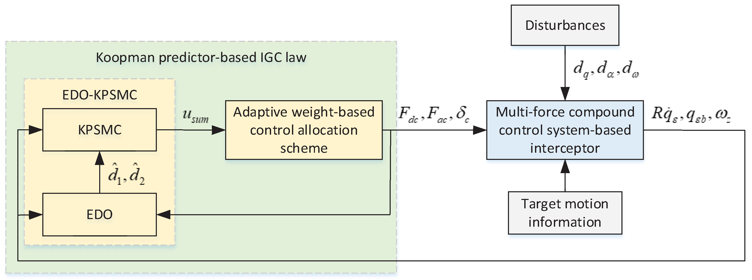
4. Koopman Predictor-Based IGC Law

The controller is designed based on the linear IGC model, which significantly reduces the design difficulty compared to the original nonlinear model. However, the modeling errors and the unknown mismatched uncertainties shown in Equations (6) and (7) lead to the differences between the model and the actual situation. The IGC model shown in Equation (21) is overdriven with more inputs than controlled outputs. Therefore, as shown in Figure 5, the proposed Koopman predictor-based IGC law is composed of the extended disturbance observer (EDO), Koopman predictor-based sliding mode control (KPSMC) and adaptive weight-based control allocation scheme. The EDO is introduced into the KPSMC law for estimating and compensating the unknown uncertainties including the modeling errors, and the EDO-based KPSMC (EDO-KPSMC) is designed for determining the required force and moment increments, while the adaptive weight-based control allocation scheme is proposed to optimize the control inputs of the multi-force compound control system under constraints and connected to the EDO-KPSMC by ${\mathit{u}}_{sum}$.

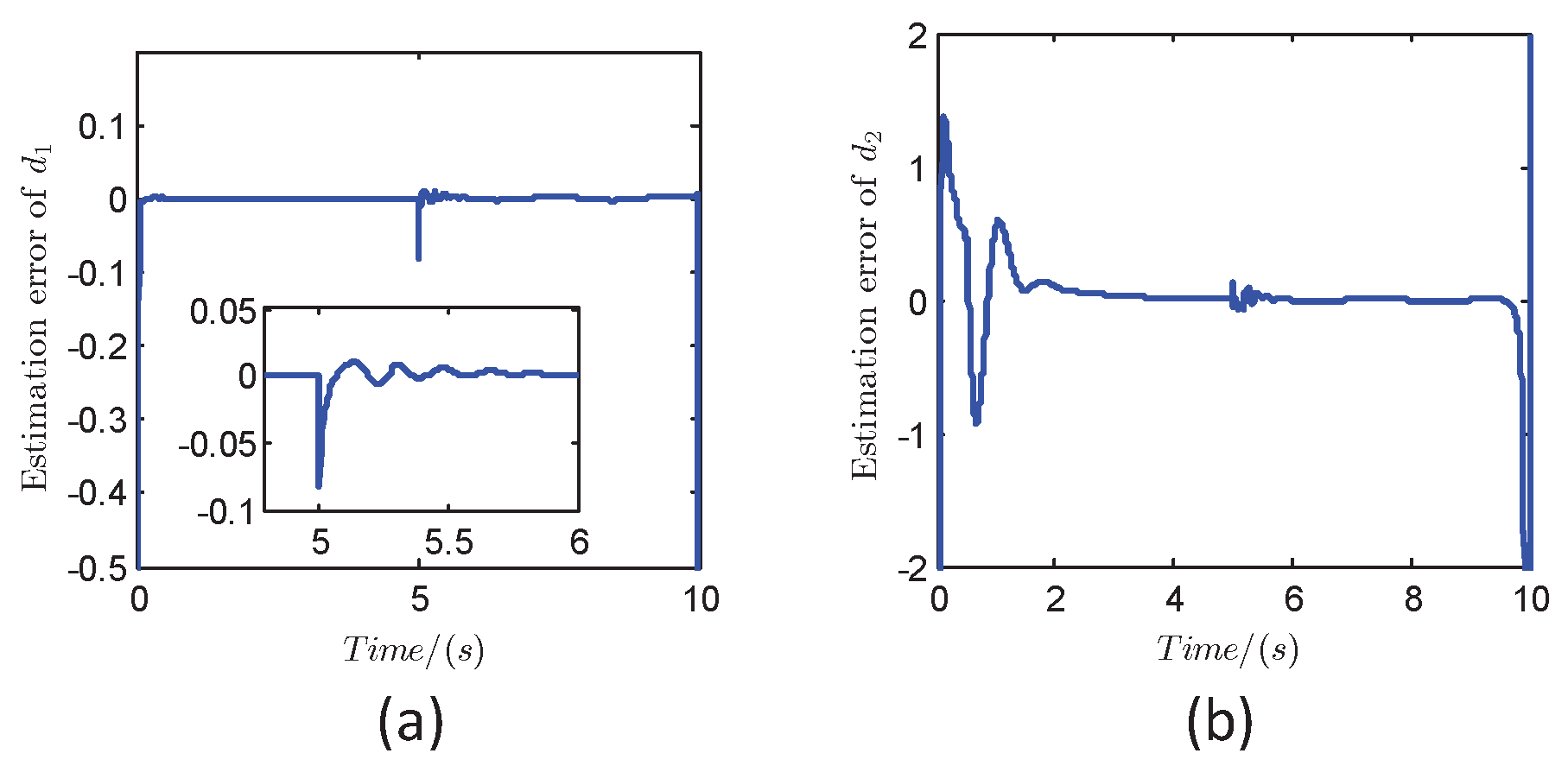
4.1. EDO for Koopman Predictor-Based IGC System

Assumption 1.

In the linear IGC model Equation (21), the unknown uncertainties and their derivatives are bounded, i.e., $\left|d_i\right|\le {\mathit{D}}_{max}$, where $i=1,2$ and ${\mathit{D}}_{max}$ is a positive constant.

According to [32], the EDO is described as follows:

$$\left.\begin{array}{cc}\hfill & {\widehat{d}}_i\left(t\right)={\mu }_{i1}\left(t\right)+{\lambda }_{i1}{\mathit{x}}_i\left(t\right)\hfill \\ \hfill & {\widehat{\dot{d}}}_i\left(t\right)={\mu }_{i2}\left(t\right)+{\lambda }_{i2}{\mathit{x}}_i\left(t\right)\hfill \\ \hfill & {\dot{\mu }}_{i1}\left(t\right)=-{\lambda }_{i1}{\widehat{\dot{\mathit{x}}}}_i\left(t\right)+{\widehat{\dot{d}}}_i\left(t\right)\hfill \\ \hfill & {\dot{\mu }}_{i2}\left(t\right)=-{\lambda }_{i2}{\widehat{\dot{\mathit{x}}}}_i\left(t\right)\hfill \end{array}\right\}$$

(22)

where ${\widehat{d}}_i$ and ${\widehat{\dot{d}}}_i$ are the estimations of $d_i$ and ${\dot{d}}_i$, respectively. ${\mu }_{i1}$ and ${\mu }_{i2}$ are auxiliary variables. ${\lambda }_{i1}$ and ${\lambda }_{i2}$ are positive constants. The difference between ${\widehat{\dot{\mathit{x}}}}_i$ and ${\dot{\mathit{x}}}_i$ is that the uncertainties in ${\widehat{\dot{\mathit{x}}}}_i$ are estimated rather than real. Hence, defining ${\tilde{d}}_i=d_i-{\widehat{d}}_i$, there is ${\dot{\mathit{x}}}_i-{\widehat{\dot{\mathit{x}}}}_i={\tilde{d}}_i$.

Lemma 1

([32]). After a sufficiently long time, the estimation errors can be bounded to the desired range with proper parameters ${\lambda }_{i1}$ and ${\lambda }_{i2}$ as follows:

$$∥{\tilde{e}}_i∥\le {\displaystyle \frac{2∥P_i{N}_i∥{\mathit{D}}_{max}}{{\lambda }_s}}$$

(23)

where $N_i=\left[\begin{array}{c}1\\ 0\end{array}\right]$, the values of $P_i$ and ${\lambda }_s$ depend on ${\lambda }_{i1}$ and ${\lambda }_{i2}$.

See the proof and detailed description in Appendix A.

Remark 4.

To compensate for the modeling error caused by the Koopman predictor-based linearization, the EDO is constructed based on the original nonlinear model.

4.2. KPSMC-Based IGC Law Under Multi-Force Compound Control

To facilitate the control law design for the strongly coupled, high-order, and strongly nonlinear system, the Koopman predictor for the interceptor under multi-force compound control is proposed in Section 3. With the help of the Koopman predictor, the original complex system is transformed into a first-order linear system as Equation (21).

Due to the sampling time $\tau$ in the calculation and measurement, the data collected to construct the Koopman predictor are discrete, so the essence of the proposed linear IGC system Equation (21) is a discrete system. Unlike the general sliding mode control (SMC) law for the continuous systems, the SMC law for the Koopman predictor-based linear IGC system needs to strictly fit the sampling time of the Koopman predictor. On this basis, the KPSMC is designed in this section.

It is desired that the BLOS angle is in the middle of the field of view (FOV) of the strapdown seeker, so there is $q_{\epsilon \mathit{B}}=q_c$, where $q_c$ is the centerline of the FOV. Assuming that the strapdown seeker is symmetric, there is $q_c=0$. Meanwhile, it is desired that $R{\dot{q}}_{\epsilon }=0$, representing that the target is intercepted. Based on the above requirements, the sliding mode surface for the linear IGC system Equation (21) is designed as follows:

$$\mathit{S}\left(t\right)=\left[\begin{array}{c}{s}_1\left(t\right)\\ s_2\left(t\right)\end{array}\right]=\left[\begin{array}{c}{q}_{\epsilon b}\\ R{\dot{q}}_{\epsilon }\end{array}\right]$$

(24)

According to Equation (21), predicting $\mathit{S}(t+\tau )$ at the next sampling moment yields

$$\begin{array}{cc}\hfill \Delta \mathit{S}\left(t\right)& =\mathit{S}(t+\tau )-\mathit{S}\left(t\right)\hfill \\ \hfill & =\overline{\mathit{C}}\mathit{A}{\mathit{x}}_{lift}\left(t\right)+\overline{\mathit{C}}\mathit{Bu}\left(t\right)+\mathit{D}-\mathit{S}\left(t\right)\hfill \end{array}$$

(25)

Considering the inevitable estimation errors of EDO, the reaching law is designed as follows:

$$\Delta {\mathit{S}}_c\left(t\right)=\left[\begin{array}{c}-k_{11}\tau s_1\left(t\right)-k_{12}\tau {\displaystyle \frac{s_1\left(t\right)}{\left|s_1\left(t\right)\right|+{\sigma }_1}}\\ -k_{21}\tau s_2\left(t\right)-k_{22}\tau {\displaystyle \frac{s_2\left(t\right)}{\left|s_2\left(t\right)\right|+{\sigma }_2}}\end{array}\right]+\tilde{\mathit{D}}$$

(26)

where $\tilde{\mathit{D}}={\left[\begin{array}{cc}{\tilde{d}}_1& {\tilde{d}}_2\end{array}\right]}^T$. $\Delta {\mathit{S}}_c$ is the desired $\Delta \mathit{S}$. $k_{i1}$, $k_{i2}$ and ${\sigma }_i$ are positive constants, where $i=1,2$.

Let $\Delta \mathit{S}\left(t\right)=\Delta {\mathit{S}}_c\left(t\right)$. Substituting Equation (26) into Equation (25) yields the EDO-KPSMC law as follows:

$$\overline{\mathit{C}}\mathit{Bu}\left(t\right)=\Delta {\mathit{S}}_c+\mathit{S}\left(t\right)-\widehat{\mathit{D}}-\overline{\mathit{C}}\mathit{A}{\mathit{x}}_{lift}\left(t\right)$$

(27)

where $\widehat{\mathit{D}}={\left[\begin{array}{cc}{\widehat{d}}_1& {\widehat{d}}_2\end{array}\right]}^T$. $\overline{\mathit{C}}\mathit{B}$ is a matrix of size $2\times 3$, representing that Equation (27) is an overdriven control system, including three control inputs and two controlled outputs. $\overline{\mathit{C}}\mathit{Bu}$, denoted as ${\mathit{u}}_{sum}$, is determined by the sum of the required force and moment increments that needs to be generated by the multi-force compound control system. There are countless schemes for the multi-force compound control system to realize ${\mathit{u}}_{sum}$, but considering the input saturation and limited engine fuel, it is essential to combine the EDO-KPSMC law with a control allocation scheme to optimize the control commands of the divert thrust, attitude thrust, and rudder deflection. The proposed control allocation scheme is shown in Section 4.3.

Theorem 1.

For the linear IGC system Equation (21) under the EDO-KPSMC law Equation (27), when ${\sigma }_i>{\displaystyle \frac{k_{i2}\tau }{2-k_{i1}\tau }}$, the controlled outputs are boundedly stable, and the convergence ranges are given as follows:

$$\left|y_i\left(t\right)\right|\le \left|{\displaystyle \frac{-\left|{\Gamma }_i\right|{\mathit{D}}_{max}+\sqrt{\left(2{\Gamma }_i^2-1\right){\mathit{D}}_{max}^2}}{\left({\Gamma }_i^2-1\right)}}\right|$$

(28)

where ${\Gamma }_i=1-k_{i1}\tau -{\displaystyle \frac{k_{i2}\tau }{\left|s_i\left(t\right)\right|+{\sigma }_i}}$.

Proof. 

Choose a Lyapunov function as $V\left(t\right)=\mathit{S}\left(t\right){\mathit{S}}^T\left(t\right)$ and define $\Delta V\left(t\right)=V(t+\tau )-V\left(t\right)$. Substituting Equation (26) into $\Delta V\left(t\right)$ yields

$$\begin{array}{cc}\hfill \Delta V\left(t\right)& =\left[\mathit{S}\left(t\right)+\Delta {\mathit{S}}_c\left(t\right)\right]{\left[\mathit{S}\left(t\right)+\Delta {\mathit{S}}_c\left(t\right)\right]}^T-\mathit{S}\left(t\right){\mathit{S}}^T\left(t\right)\hfill \\ \hfill & ={\left[{\Gamma }_1{s}_1\left(t\right)+{\tilde{d}}_1\right]}^2+{\left[{\Gamma }_2{s}_2\left(t\right)+{\tilde{d}}_2\right]}^2-s_1^2-s_2^2\hfill \\ \hfill & \le \left({\Gamma }_1^2-1\right){\left|s_1\left(t\right)\right|}^2+2\left|{\Gamma }_1\right|\left|s_1\left(t\right)\right|{\mathit{D}}_{max}+{\mathit{D}}_{max}^2\hfill \\ \hfill & +\left({\Gamma }_2^2-1\right){\left|s_2\left(t\right)\right|}^2+2\left|{\Gamma }_2\right|\left|s_2\left(t\right)\right|{\mathit{D}}_{max}+{\mathit{D}}_{max}^2\hfill \end{array}$$

(29)

where ${\Gamma }_i=1-k_{i1}\tau -{\displaystyle \frac{k_{i2}\tau }{\left|s_i\left(t\right)\right|+{\sigma }_i}}$, $i=1,2$.

Observing the structure of Equation (29), it can be viewed as two quadratic equations with $\left|s_1\left(t\right)\right|$ and $\left|s_2\left(t\right)\right|$ as variables as follows:

$$f\left(s_i\right)=\left({\Gamma }_i^2-1\right){\left|s_i\left(t\right)\right|}^2+2\left|{\Gamma }_i\right|\left|s_i\left(t\right)\right|{\mathit{D}}_{max}+{\mathit{D}}_{max}^2$$

(30)

Based on Veda’s theorem, since ${\mathit{D}}_{max}>0$, there must be two real roots denoted as $o_{i1}$ and $o_{i2}$, where $o_{i1}>o_{i2}$. If ${\Gamma }_i^2-1\ge 0$, there is $\Delta V\left(t\right)\ge 0$ when $\left|s_i\left(t\right)\right|\to \infty$, implying that the controlled system is unstable. Hence, ${\Gamma }_i^2-1<0$ is the prerequisite for the controlled system to be stable. Because $k_{i1}$, $k_{i2}$, ${\sigma }_i$ and $\tau$ are positive constants, when ${\sigma }_i>{\displaystyle \frac{k_{12}\tau }{2-k_{11}\tau }}$, ${\Gamma }_i^2-1<0$ always holds. In fact, the relationship between $\Delta V\left(t\right)$ and $\left|s_i\left(t\right)\right|$ can be described as parabolas with the opening facing down. ${\Gamma }_i^2-1<0$ and $-{\displaystyle \frac{2\left|{\Gamma }_i\right|{\mathit{D}}_{max}}{{\Gamma }_i^2-1}}>0$ imply that $o_{i1}>0$ and $\left|o_{i1}\right|>\left|o_{i2}\right|$. so when $\left|s_i\left(t\right)\right|>o_{i1}$, $\Delta V\left(t\right)<0$ always holds. Therefore, combining Equations (24) and (30), the convergence ranges of the controlled outputs are given as follows:

$$\left|y_i\left(t\right)\right|\le {\displaystyle \frac{-\left|{\Gamma }_i\right|{\mathit{D}}_{max}+\sqrt{\left(2{\Gamma }_i^2-1\right){\mathit{D}}_{max}^2}}{\left({\Gamma }_i^2-1\right)}}$$

(31)

where $y_1=q_{\epsilon b}$ and $y_2=R{\dot{q}}_{\epsilon }$. □

Remark 5.

The control allocation scheme is designed subject to satisfying Equation (27), so the stability and convergence range of the controlled system is not affected by the control allocation scheme.

4.3. Adaptive Weight-Based Control Allocation Scheme

According to Equation (27), the IGC system under the multi-force compound control system consisting of the divert thrust, attitude thrust, and rudder deflection is overdriven. The control allocation scheme is proposed to coordinate multiple actuators to generate the desired force and moment while ensuring that the actuators are able to fulfill the control commands. Thus, the cost function for the overdriven control system Equation (27) is designed as follows:

$$\begin{array}{cc}\hfill & J=min{\displaystyle \frac{1}{2}}{\mathit{u}}^T\left(t\right)\mathit{W}\mathit{u}\left(t\right)\hfill \\ \hfill & \mathrm{subject}\mathrm{to}\mathrm{Equations}\left(4\right)\left(5\right)\mathrm{and}\left(27\right)\hfill \end{array}$$

(32)

where $\mathit{W}$ is the weight matrix. Equation (27) is the total required input based on the EDO-KPSMC law. Equation (4) represents the input saturations. Equation (5) represents the total fuel constraints for the divert thrust and attitude thrust. Equation (27) is an equality constraint, and Equations (4) and (5) are inequality constraints.

Remark 6.

Generally, the weight matrix of the cost function for the control allocation scheme is constant, and the value of it is determined by the control efficiency of each actuator in the flight environment. However, generating divert thrust or attitude thrust requires continuous fuel consumption. The constant weight matrix cannot reflect the time-varying remaining fuel, making it difficult to allocate the fuel reasonably throughout the terminal guidance phase.

The existence of inequality constraints makes it difficult to directly calculate the analytical solution of $\mathit{u}$, resulting in high computation burden. The adaptive weight matrix incorporating inequality constraints is proposed to reduce the computation burden and improve the performance of the overdriven control system under the multi-force compound control. The control commands are determined in conjunction with real-time actuator states.

According to the inequality constraints shown in Equations (4) and (5), the design of the adaptive weight matrix starts from the following aspects:

(1)

Normalize the input range of actuators. Describing the control inputs in terms of a uniform standard, the control inputs are subjected to the following normalization transformation:

$${\overline{\mathit{u}}}_i={\displaystyle \frac{{\mathit{u}}_i}{{\mathit{u}}_{imax}}}$$

(33)

where ${\overline{\mathit{u}}}_i\in \left[-1,1\right]$ is the normalized control input. ${\mathit{u}}_{imax}$ is the maximum control input, $i=1,2,3$, representing the $F_{d max}$, $F_{a max}$, and ${\delta }_{max}$ in the multi-force compound control, respectively.

Equation (33) transforms the absolute control input into the relative control input. Introducing the normalized control inputs into the adaptive weights is helpful for improving the fairness of the control allocation.

(2)

Coordinate the residual control capability. The control allocation scheme needs to avoid input saturation as much as possible. Additionally, considering that the fuel-consuming and non-fuel-consuming actuators simultaneously exist in the multi-force compound control system, the fuel margin should be considered in the control allocation scheme to avoid premature fuel exhaustion.

Based on the above requirements, an adaptive weight based on a quadratic function with real-time control input as the benchmark is proposed as follows:

$$w_i(t+\tau )={\psi }_i\left(t\right){\overline{\mathit{u}}}_i^2\left(t\right)+\xi$$

(34)

where $i=1,2,3$, $\mathit{W}\left(\mathit{t}\right)=\mathrm{diag}({\mathit{w}}_1\left(t\right),w_2\left(t\right),w_3\left(t\right))$ and the initial of it is $\mathit{W}\left(0\right)=\mathrm{diag}(\xi ,\xi ,\xi )$. The meanings of ${\psi }_i\left(t\right)$ and $\xi$ are shown in Figure 6. $\xi$ is a positive constant used as the base weight to avoid the weight being zero. ${\psi }_i\left(t\right)$ is a function determined by the consumed fuel as follows:

$$\begin{array}{cc}\hfill & {\psi }_1\left(t\right)=\left[1+{\displaystyle \frac{I_d\left(t\right)}{I_{dsum}}}\right]\gamma \hfill \\ \hfill & {\psi }_2\left(t\right)=\left[1+{\displaystyle \frac{I_a\left(t\right)}{I_{asum}}}\right]\gamma \hfill \\ \hfill & {\psi }_3\left(t\right)=\gamma \hfill \end{array}$$

(35)

where $\gamma$ is a positive adjustment parameter. $I_d$, $I_a$, $I_{dsum}$, and $I_{asum}$ are defined in Equation (5).

Remark 7.

Since Equation (34) is designed for the normalized control inputs, the values of ξ and ϕ are constant in the calculation of the weights for the three control inputs.

The main objective of the proposed adaptive weight is to ensure that the control commands are realizable without introducing the inequality constraints of Equations (4) and (5) directly into the cost function Equation (32). According to Equations (33)–(35), it can be analyzed that when the control input is closer to the maximum value, the corresponding weight coefficient is larger; when the remaining fuel is less, the weight coefficient of the divert thrust or attitude thrust is larger.

With the help of the proposed adaptive weight matrix, the cost function Equation (32) can be rewritten as

$$\begin{array}{cc}\hfill & J=min{\displaystyle \frac{1}{2}}{\mathit{u}}^T\left(t\right)\mathit{W}\left(t\right)\mathit{u}\left(t\right)\hfill \\ \hfill & \mathrm{subject}\mathrm{to}\mathrm{Equation}\left(27\right)\hfill \end{array}$$

(36)

Therefore, the analytical solution for the control inputs under the overdriven control system can be obtained as follows:

$$\mathit{u}\left(t\right)={\mathit{W}}^{-1}\left(t\right){\left(\overline{\mathit{C}}\mathit{B}\right)}^T{\left[\left(\overline{\mathit{C}}\mathit{B}\right){\mathit{W}}^{-1}\left(t\right){\left(\overline{\mathit{C}}\mathit{B}\right)}^T\right]}^{-1}{\mathit{u}}_{sum}\left(t\right)$$

(37)

where ${\mathit{u}}_{sum}$ is obtained based on the EDO-KPSMC law of Equation (27).

5. Simulation Studies

The installation and dynamic parameters of the actuators are set as ${\mathit{x}}_d=0.48\mathrm{m}$, ${\mathit{x}}_a=0.1\mathrm{m}$, $F_{d max}=5000\mathrm{N}$, $F_{a max}=500\mathrm{N}$, ${\delta }_{max}=20deg$, $I_{dmax}=15,000\mathrm{N}·\mathrm{s}$, $I_{amax}=1500\mathrm{N}·\mathrm{s}$, ${\omega }_{\delta }=6$, $\xi =0.7$, ${\tau }_d=0.15$ and ${\tau }_a=0.1$. The parameters of the interceptor are set as ${\mathit{x}}_G=0.5\mathrm{m}$, $L=1\mathrm{m}$, $S=0.05{\mathrm{m}}^2$, $m=50\mathrm{kg}$, $J_z=15\text{kg}·{\mathrm{m}}^2$, $c_y^{\alpha }=1.5$, $m_z^{\alpha }=-0.15$, $m_z^{{\omega }_z}=-0.01$ and $m_z^{\delta }=-0.125$. The flight speed of the interceptor and target are $V_M=1500\mathrm{m}/\mathrm{s}$ and $V_T=1500\mathrm{m}/\mathrm{s}$, respectively. The initial states of the interceptor and target are set as ${\mathit{x}}_m=0\mathrm{m}$, $y_m=0\mathrm{m}$, $x_t=\mathrm{30,000}\mathrm{m}$, $y_t=500\mathrm{m}$, ${\theta }_M=0\mathrm{deg}$, ${\theta }_T=180\mathrm{deg}$, and ${\omega }_z=0\mathrm{deg}/\mathrm{s}$ and $\alpha =0\mathrm{deg}$. The air density and the gravity acceleration are set as $\rho =0.088\mathrm{kg}/{\mathrm{m}}^3$, and $g=9.7\mathrm{m}/{\mathrm{s}}^2$, respectively. The parameters of the proposed controller are set as $k_{11}=1$, $k_{12}=1$, $k_{21}=20$, $k_{22}=1$, ${\tau }_1={\tau }_2=1$, ${\lambda }_{21}={\lambda }_{22}=500$, ${\lambda }_{11}={\lambda }_{12}=100$. The sampling time is set as 5 ms.

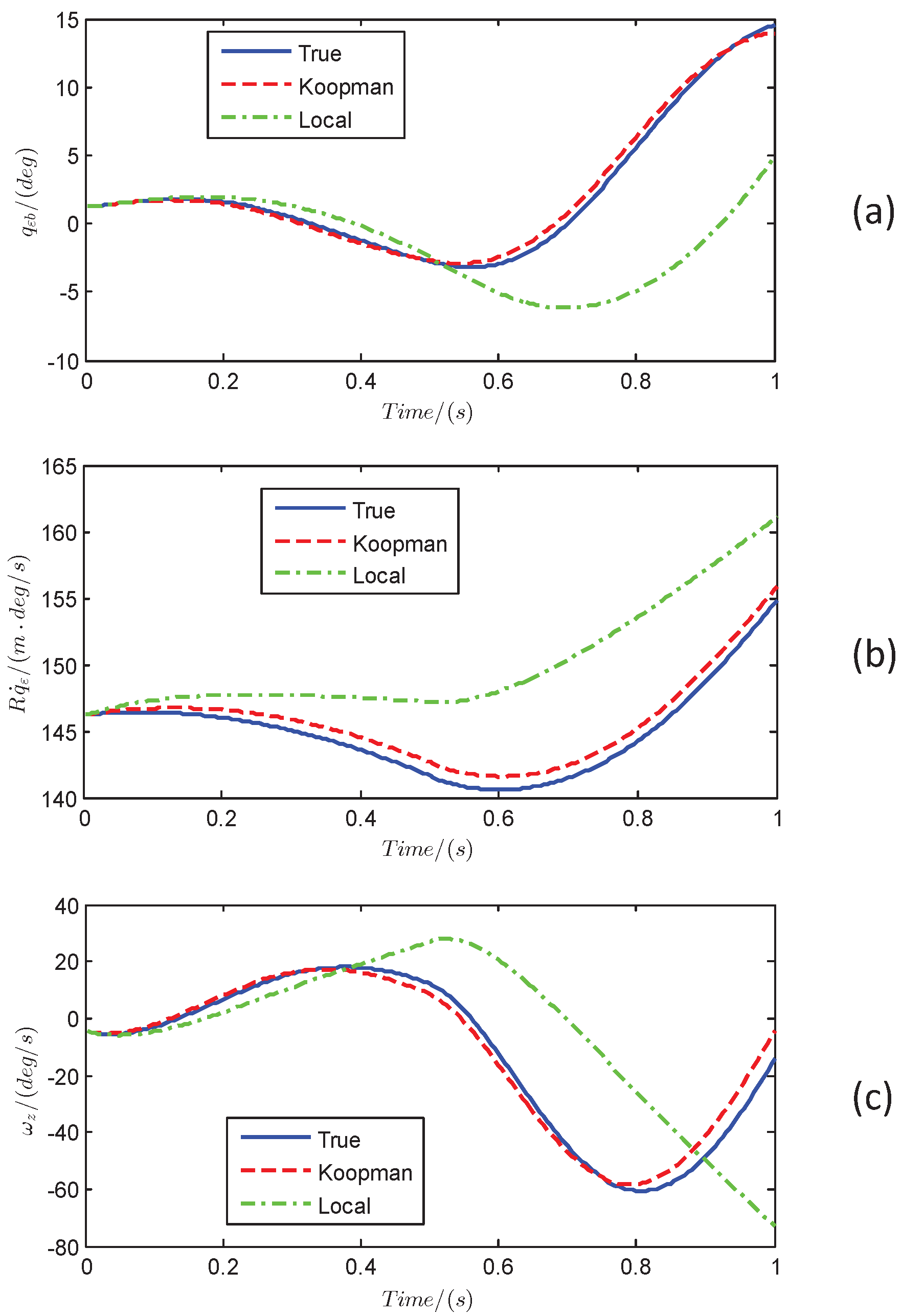
5.1. Accuracy of Koopman Predictor

The construction of the Koopman predictor-based linear IGC model is proposed in Section 3.2. Before designing the control law, it is necessary to verify the accuracy of the Koopman predictor, that is, the reliability of the linear IGC model. The raw data for training the Koopman predictor are collected from simulation tests. The fourth-order Runge–Kutta is used to discretize the dynamics with the sampling time $T=5\mathrm{ms}$. The parameters for data collection are set as $N_s=1600$ and $N_t=500$, representing that simulating 500 trajectories with 8 s (1600 sampling periods) per trajectory. The parameter for determining the lifted states is set as $N_c=100$, representing that the dimension of the state-space is lifted from 3 to 103. The 100 center points are selected randomly with uniform distribution on the unit box. The parameters for adjusting the range of states are set as ${\epsilon }_1=1$, ${\epsilon }_2=0.01$, and ${\epsilon }_3=1$.

The accuracy of the Koopman predictor is verified by comparing the simulation results with the local linearization-based predictor. The local linearization is achieved based on the first-order Taylor series expansion of the dynamics. In the comparison simulation, the control inputs are set as $F_{dc}=0.1F_{d max}\mathrm{sign}\left(sin\left(2\pi t\right)\right)$, $F_{ac}=0.1F_{a max}\mathrm{sign}\left(sin\left(2\pi t\right)\right)$, and ${\delta }_c=0.1{\delta }_{max}\mathrm{sign}\left(sin\left(2\pi t\right)\right)$. To make the simulation result reliable, the initial states and control inputs for the Koopman predictor and the local linearization-based predictor are the same.

The relative root mean squared error (RMSE) is used to quantitatively evaluate the prediction accuracy for each predictor averaged over 100 randomly sampled initial conditions with the same control inputs as follows:

$$\mathrm{RMSE}=100·{\displaystyle \frac{\sqrt{{\displaystyle \sum _{i=1}^{N_p}}{∥{\mathit{x}}_{pred}\left(k\right)-{\mathit{x}}_{true}\left(k\right)∥}_2^2}}{{\displaystyle \sum _{i=1}^{N_p}}{∥{\mathit{x}}_{true}\left(k\right)∥}_2^2}}$$

(38)

where $N_p=200$ represents the number of predicted sampling periods. ${\mathit{x}}_{pred}$ and ${\mathit{x}}_{true}$ are the predicted states and the true states, respectively.

Figure 7 shows the predicted state curves in 1 s; it can be observed that compared to the local linearization-based predictor, the states predicted by the Koopman predictor are closer to the true value. Based on Equation (38), it can be calculated that the RMSE of the Koopman predictor and local linearization-based predictor are $3.37\%$ and $45.25\%$, implying that the accuracy of the Koopman predictor is higher than the local linearization-based predictor. The simulation results demonstrate that the Koopman predictor has higher accuracy, so it is feasible to replace the original nonlinear model with the Koopman predictor-based linear IGC model for designing the IGC law.

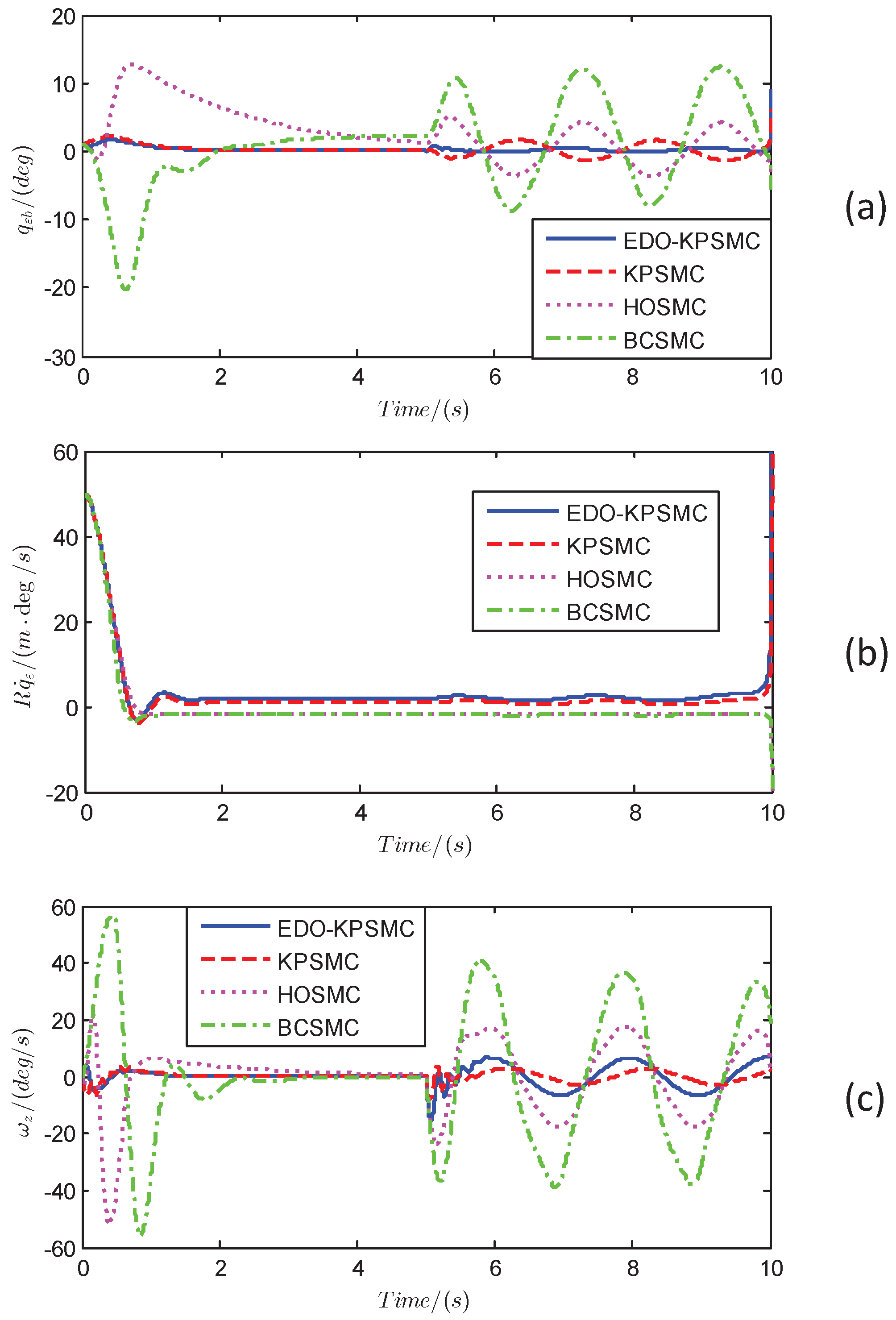
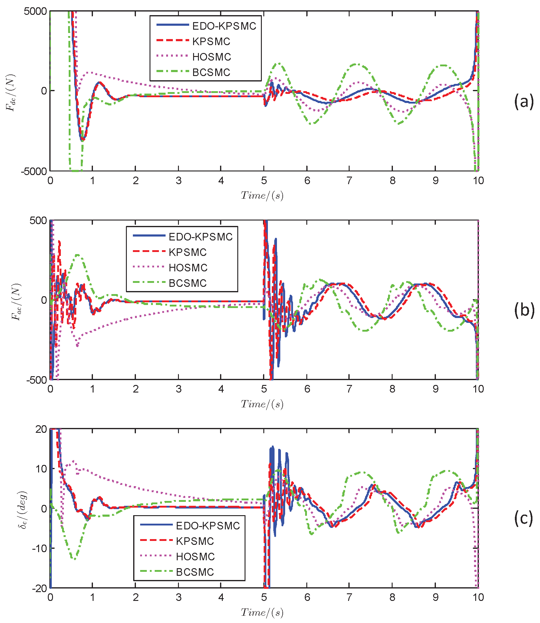
5.2. Effectiveness of EDP-KPSMC

The effectiveness of EDO-KPSMC is verified by comparing the simulation results with the KPSMC, high-order sliding mode control (HOSMC) [19], and backstepping control-based sliding mode control (BCSMC) [33]. To avoid the influence of the control allocation scheme on the result, all control laws in the comparison simulation adopt the same control allocation scheme.

The KPSMC is Equation (37) with $\widehat{D}=0$. The BCSMC is designed order by order based on the reaching law $\dot{s}=-k_{1}s-k_2{\displaystyle \frac{s}{\left|s\right|+\tau }}$, where $k_1$ and $k_2$ are positive constants. The low-pass filter ${\displaystyle \frac{1}{Ts+1}}$ is introduced to deal with the “exponential explosion” issue in BC-based controllers. The essence of BC is to decompose the high-order system into multiple independent first-order subsystems, so the couplings in multi-force compound control system are ignored in BCSMC. Considering the trajectory and attitude control systems as a high-order multi-dimensional interconnected system, the sliding mode matrix of the HOSMC is designed as $\mathit{S}=\left[\begin{array}{c}{s}_1\\ s_2\end{array}\right]=\left[\begin{array}{c}f\left(q_{\epsilon b}\right)\\ f\left(R{\dot{q}}_{\epsilon }\right)\end{array}\right]$.

The couplings caused by the multi-force compound control system are considered in the HOSMC. However, the relative order of each control input to the controlled output is different, which makes it difficult for the HOSMC to consider the dynamics of the actuators in the design. Thus, in the comparison simulation, the independent servo systems are introduced to compensate for the response delay of actuators.

To enhance the reliability of the comparison simulation, the EDO-KPSMC, KPSMC, HOSMC, and BCSMC are designed with the same reaching law. Meanwhile, to comprehensively compare the performance of the above four control laws, the simulation is completed in the presence of the unknown uncertainties $d_{\omega }=5cos\left(\pi t\right)deg/\mathrm{s}$, $\Delta a_T=10 \mathrm{m}/{\mathrm{s}}^2$ and $\Delta q_{\epsilon b}=2sin\left(\pi t\right)deg$ appearing after 5 s.

The state curves and input curves are shown in Figure 8 and Figure 9, respectively. It can be seen that the BLOS angle and the attitude under the EDO-KPSMC and KPSMC are more stable than the HOSMC and BCSMC, the BCSMC has the worst stabilizing ability in the presence of unknown uncertainties, and the uncertainty suppression ability of KPSMC is significantly enhanced with the help of EDO. As shown in Figure 8b, compared to the HOSMC and BCSMC designed based on the original nonlinear model, the static difference is inevitable with the EDO-KPSMC and KPSMC designed based on the linear IGC model because of the linearization error. The estimation errors are shown in Figure 10. It can be observed that the estimation errors converge to zero before 5 s, and the estimation errors fluctuate due to the sudden appearance of the unknown uncertainties but quickly converge to zero again.

Table 1. Interception state and engine consumption under EDO-KPSMC, KPSMC, HOSMC, and BCSMC.

	EDO-KPSMC	KPSMC	HOSMC	BCSMC
Miss distance (m)	0.37	0.25	0.12	0.10
Divert thrust impulse ($\mathrm{kN}·\mathrm{s}$)	5.87	5.83	7.54	8.99
Attitude thrust impulse ($\mathrm{kN}·\mathrm{s}$)	0.47	0.50	0.78	0.79

displays the miss distance, divert thrust impulse, and attitude thrust impulse under these control laws. It can be analyzed that the interceptor can successfully hit the target under all control laws, but the thrust impulses of EDO-KPSMC and KPSMC are significantly less compared to HOSMC and BCSMC, meaning that the EDO-KPSMC and KPSMC consume less fuel.

According to the above simulation results, it can be concluded that the more comprehensive the consideration of the input couplings and the dynamic characteristics of the actuators in the control law design, and the higher the integration degree of the guidance, attitude control and actuator response, the higher the fuel utilization efficiency and the more robust the control system.

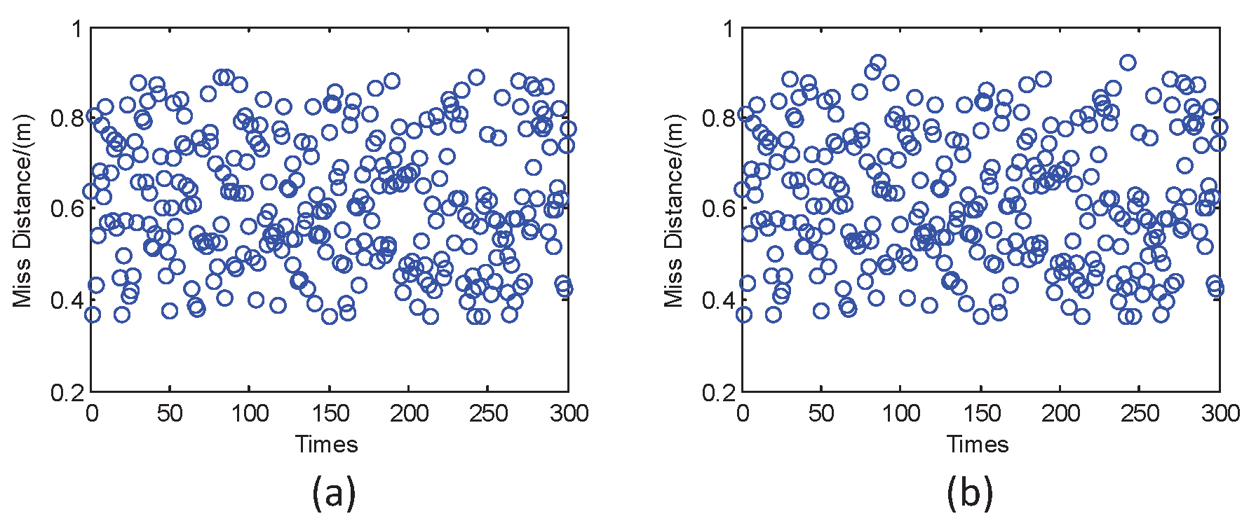
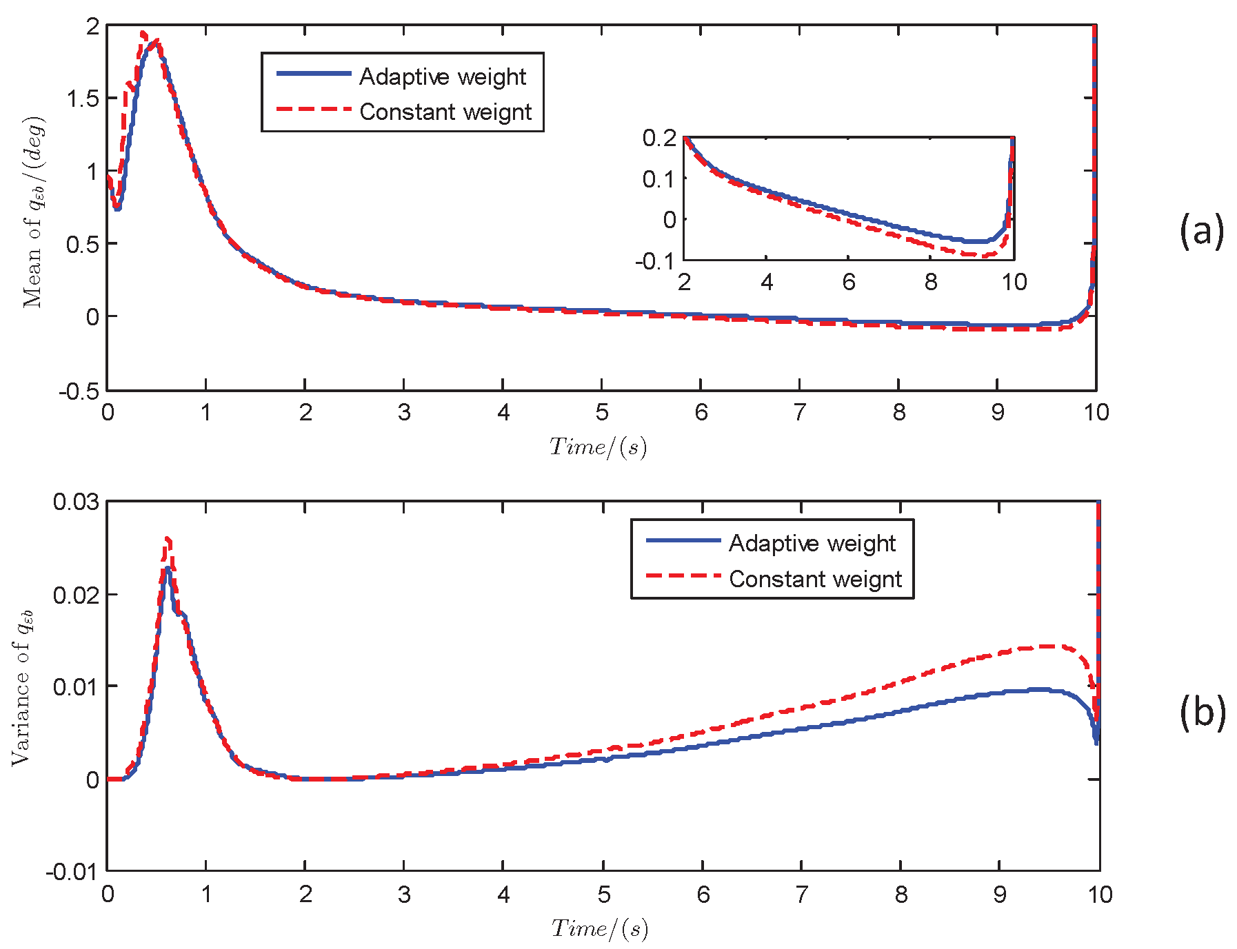
5.3. Effectiveness of Adaptive Weight-Based Control Allocation Scheme

Monte Carlo tests under the EDO-KPSMC law are utilized to compare the control allocation scheme based on the adaptive weights and constant weights. In the 300 times Monte Carlo test, the parameter perturbations are $\left|\Delta c_y^{\alpha }\right|\le 10\%$, $\left|\Delta m_z^{\alpha }\right|\le 15\%$ and $\left|\Delta m_z^{{\omega }_z}\right|\le 50\%$, the unknown target maneuver is $\left|\Delta a_T\right|\le 5\mathrm{m}/{\mathrm{s}}^2$, and the measurement error of the seeker is $\left|\Delta q_{\epsilon b}\right|\le 2deg$. The constant weight is set as $w_i={\displaystyle \frac{1}{{\mathit{u}}_{imax}}}$, where ${\mathit{u}}_{imax}$ is the maximum control input of each actuator. The mean and variance of the Monte Carlo tests are represented as $E\left[{\mathit{x}}_i\left(k\right)\right]={\displaystyle \frac{1}{300}}{\displaystyle \sum _{k=1}^{300}}{\mathit{x}}_i\left(k\right)$ and $D\left[{\mathit{x}}_i\left(k\right)\right]={\displaystyle \frac{1}{300}}{\displaystyle \sum _{k=1}^{300}}{\left\{{\mathit{x}}_i\left(k\right)-E\left[{\mathit{x}}_i\left(k\right)\right]\right\}}^2$, respectively.

The miss distance with the adaptive weights and constant weights is shown in Figure 11, the mean and variance of BLOS angle are shown in Figure 12, and the mean of miss distance and engine consumption with adaptive weights and constant weights are shown in

Table 2. Mean of miss distance and engine consumption with adaptive weights and constant weights.

	Adaptive Weight	Constant Weight
Miss distance (m)	0.62	0.62
Divert thrust impulse ($\mathrm{kN}·\mathrm{s}$)	8.31	8.47
Attitude thrust impulse ($\mathrm{kN}·\mathrm{s}$)	0.62	0.78

. According to Figure 11 and Table 2, it can be seen that the miss distance is almost unaffected by the control allocation schemes, but replacing the constant weights with adaptive weights can effectively reduce the consumption of fuel. Combining the kinematics and dynamics of the interceptor under the multi-force compound control, it can be analyzed that the function of the orbit control engine is irreplaceable, and the function between the attitude control engine and aerodynamic rudder is highly replaceable. Thus, compared to the divert thrust, the attitude thrust and rudder deflection are more affected by the control allocation schemes. It can be calculated based on the data shown in Table 2 that the constant weight-based control allocation scheme uses an average of $1.93\%$ more divert impulse and $25.81\%$ more attitude impulse than the adaptive weight.

Although the ability of the interceptor to accurately hit the target mainly depends on the control law, the adaptive weight-based control allocation scheme can efficiently coordinate the actuators to reduce fuel consumption while generating the required force and moment, which is helpful for fuel limited interceptors. In summary, the results of the Monte Carlo tests not only verify the effectiveness of the adaptive weight-based control allocation scheme but also further demonstrate the robustness of the EDO-KPSMC law against unknown uncertainties.

6. Conclusions

This paper proposes a Koopman predictor-based IGC law for the hypersonic target interceptor under the multi-force compound control. The kinematics and dynamics model of the interceptor is established by combining the physical limitations, working principles and dynamic characteristics of the aerodynamic rudder, attitude control engine, and orbit control engine. To simplify the guidance and control system while satisfying the model accuracy, the data-driven Koopman predictor is constructed, and the linear IGC model under the multi-force compound control considering the high-order, strong coupling and strong nonlinearity features is established. Then, the proposed Koopman predictor-based IGC law is designed based on the KPSMC for nominal control, the EDO for estimating and compensating for the mismatched unknown uncertainties, and the adaptive weight-based control allocation scheme for efficiently coordinating the actuators to reduce fuel consumption and avoid input saturation. It is proved that the system controlled by the proposed IGC law is stable. As shown in the simulations, the proposed Koopman predictor can accurately predict the response curves of the original nonlinear systems, and additionally, the proposed Koopman predictor-based IGC law can be robust against uncertainties and reduce the fuel consumption while intercepting the hypersonic targets precisely.

References

1. Ding, Y.; Yue, X.; Chen, G.S.; Si, J.S. Review of control and guidance technology on hypersonic vehicle. Chinese J. Aeronaut. 2022, 35, 1–18. [Google Scholar] [CrossRef]
2. Peng, Q.; Chen, G.; Guo, J.G.; Guo, Z.Y. Finite-time convergent sliding mode guidance Law-based capture region with multiple constraints. IEEE Trans. Aerosp. Electron. Syst. 2025. Early Access. [Google Scholar] [CrossRef]
3. Kim, S.; Cho, D.; Kim, H.J. Force and moment blending control for fast response of agile dual missiles. IEEE Trans. Aerosp. Electron. Syst. 2016, 52, 938–947. [Google Scholar] [CrossRef]
4. Zhang, Y.A.; Wu, H.L.; Liu, J.M.; Sun, Y.M. A blended control strategy for intercepting high-speed target in high altitude. Proc. Inst. Mech. Eng. Part J. Aerosp. Eng. 2018, 232, 2263–2285. [Google Scholar] [CrossRef]
5. Guo, Y.; Guo, J.H.; Liu, X.; Li, A.J.; Wang, C.Q. Finite-time blended control for air-to-air missile with lateral thrusters and aerodynamic surfaces. Aerosp. Sci. Technol. 2020, 97, 105638. [Google Scholar] [CrossRef]
6. Ashrafiuon, H. Guidance and attitude control of unstable rigid bodies with single-use thrusters. IEEE Trans. Control Syst. Technol. 2017, 25, 401–413. [Google Scholar] [CrossRef]
7. Shtessel, Y.B.; Tournes, C.H. Integrated higher-order sliding mode guidance and autopilot for dual-control missiles. J. Guid. Control Dyn. 2009, 32, 79–94. [Google Scholar] [CrossRef]
8. Lee, H.; Bang, H. Efficient thrust management algorithm for variable thrust solid propulsion system with multi-nozzles. J. Spacecr. Rockets 2020, 57, 328–345. [Google Scholar] [CrossRef]
9. Li, Z.B.; Dong, Q.L.; Zhang, X.Y.; Zhang, H.R.; Zhang, F. Field-to-view constrained integrated guidance and control for hypersonic homing missiles intercepting supersonic maneuvering targets. Aerospace 2022, 9, 640. [Google Scholar] [CrossRef]
10. Yu, X.J.; Luo, S.B.; Liu, G.Q. Integrated design of multi-constrained snake maneuver surge guidance control for hypersonic vehicles in the dive segment. Aerospace 2023, 10, 765. [Google Scholar] [CrossRef]
11. Li, Z.B.; Dong, Q.L.; Zhang, X.Y.; Gao, Y.F. Impact angle constrained integrated guidance and control for supersonic skid-toturn missiles using backstepping with global fast terminal sliding mode control. Aerosp. Sci. and Technol. 2022, 122, 107386. [Google Scholar] [CrossRef]
12. Zhao, B.; Xu, S.; Guo, J.; Jiang, R.; Zhou, J. Integrated strapdown missile guidance and control based on neural network disturbance observer. Aerosp. Sci. Technol. 2019, 84, 170–181. [Google Scholar] [CrossRef]
13. Luo, X.Y.; Song, J.; Zhao, M.F.; Li, W.L.; Wei, M.J. Integrated guidance and control for a hypersonic vehicle with disturbance and measurement noise suppression. IEEE Trans.Control Syst. Technol. 2024, 60, 7172–7184. [Google Scholar] [CrossRef]
14. Lu, N.B.; Guo, J.G.; Guo, Z.Y.; Wang, G.Q. Asymmetric BLOS constraint-involved intelligent integrated guidance and control approach for flight vehicle equipped with strapdown seeker. Adv. Space. Res. 2023, 72, 4461–4473. [Google Scholar] [CrossRef]
15. Guo, J.G.; Peng, Q.; Guo, Z.Y. SMC-Based Integrated Guidance and Control for Beam Riding Missiles with Limited LBPU. IEEE Trans. Aerosp. Electron. Syst. 2021, 57, 2969–2978. [Google Scholar] [CrossRef]
16. Zhao, B.; Feng, Z.X.; Guo, J.G. Integral barrier Lyapunov functions-based integrated guidance and control design for strap-down missile with field-of-view constraint. Trans. Inst. Meas. Control. 2021, 43, 1464–1477. [Google Scholar] [CrossRef]
17. Guo, J.G.; Zhou, Y.H.; Zhou, M. Adaptive control law based integrated guidance and control design for missile with the radome error compensation. Proc. Inst. Mech. Eng. 2024, 238, 361–371. [Google Scholar] [CrossRef]
18. Kim, H.G.; Beck, D. Integrated guidance and control for collision course stabilization of dual-controlled interceptors. Aerospace 2024, 11, 9. [Google Scholar] [CrossRef]
19. Peng, Q.; Chen, G.; Guo, J.G.; Guo, Z.Y. Attitude/orbit engine compound control for hypersonic target interceptor with discrete-time inputs and state constraints. IEEE Trans. Aerosp. Electron. Syst. 2024, 60, 4939–4951. [Google Scholar] [CrossRef]
20. Koopman, B.O. Hamiltonian systems and transformation in Hilbert space. Proc. Natl. Acad. Sci. USA 1931, 17, 315–318. [Google Scholar] [CrossRef]
21. Bevanda, P.; Sosnowski, S.; Hirche, S. Koopman operator dynamical models: Learning, analysis and control. Annu. Rev. Control 2021, 52, 197–212. [Google Scholar] [CrossRef]
22. Pan, S.W.; Duraisamy, K. On the lifting and reconstruction of nonlinear systems with multiple invariant sets. Nonlinear Dyn. 2024, 112, 10157–10165. [Google Scholar] [CrossRef]
23. Korda, M.; Mezic, I. Linear predictors for nonlinear dynamical systems: Koopman operator meets model predictive control. Automatica 2018, 93, 149–160. [Google Scholar] [CrossRef]
24. Uchida, D.; Yamashita, A.; Asama, H. Data-driven koopman controller synthesis based on the extended H2 norm characterization. IEEE Control. Syst. Lett. 2021, 5, 1795–1800. [Google Scholar] [CrossRef]
25. Zhang, X.L.; Pan, W.; Scattolini, R.; Yu, S.Y.; Xu, X. Robust tube-based model predictive control with Koopman operators. Automatica 2022, 137, 110114. [Google Scholar] [CrossRef]
26. Zhou, M.; Liu, M.F.; Hu, G.J.; Guo, Z.Y.; Guo, J.G. Koopman operator-based integrated guidance and control for strap-down high-speed missiles. IEEE Trans.Control Syst. Technol. 2024, 32, 2436–2443. [Google Scholar] [CrossRef]
27. Li, S.P.; Guo, J.G. An angle error extraction algorithm based on JADE for three-channel radar seeker system with the existence of deception jamming. Digit. Signal Process. 2022, 131, 103754. [Google Scholar] [CrossRef]
28. Han, T.; Hu, Q.L.; Wang, Q.Y.; Xin, M.; Shin, H.S. Constrained 3-D trajectory planning for aerial vehicles without range measurement. IEEE Trans. Syst. Man, Cybern. Syst. 2024, 54, 6001–6013. [Google Scholar] [CrossRef]
29. Zhou, J.; Liu, Z.Q.; Guo, J.G.; Guo, Z.Y. Three-dimensional piecewise guidance strategy for multi-UAVs guaranteeing simultaneous arrival and field-of-view constraint. Trans. Inst. Meas. Control. 2022, 44, 2248–2263. [Google Scholar]
30. Williams, M.O.; Kevrekidis, I.G.; Rowley, C.W. A data–driven approximation of the Koopman operator: Extending dynamic mode decomposition. J. Nonlinear Sci. 2015, 25, 1307–1346. [Google Scholar] [CrossRef]
31. Korda, M.; Mezic, I. On convergence of extended dynamic mode decomposition to the Koopman operator. J. Nonlinear Sci. 2018, 28, 687–710. [Google Scholar] [CrossRef]
32. Ginoya, D.; Shendge, P.D.; Phadke, S.B. Sliding mode control for mismatched uncertain systems using an extended disturbance observer. IEEE Trans. Ind. Electron. 2014, 61, 1983–1992. [Google Scholar] [CrossRef]
33. Peng, Q.; Guo, J.G.; Zhou, J. Integrated guidance and control system design for laser beam riding missiles with relative position constraint. Aerosp. Sci. Technol. 2020, 98, 105693. [Google Scholar] [CrossRef]
Figure 1. Mounting positions of the aerodynamic rudder, attitude control engine, and orbit control engine.
Aerospace 12 00213 g001
Figure 2. Desired effects of the multi-force compound control system.
Aerospace 12 00213 g002
Figure 3. Actual effects of the multi-force compound control system.
Aerospace 12 00213 g003
Figure 4. Interceptor–target engagement geometry under multi-force compound control in longitudinal plane.
Aerospace 12 00213 g004
Figure 5. Schematic diagram of the proposed IGC law.
Aerospace 12 00213 g005
Figure 6. Schematic diagram of adaptive weight determination.
Aerospace 12 00213 g006
Figure 7. Predicted state curves in 1 s: (a) BLOS angle. (b) Product of the interceptor−target relative distance and LOS angular rate. (c) Angular pitch rate.
Aerospace 12 00213 g007
Figure 8. State curves in the presence of unknown uncertainties under EDO−KPSMC, KPSMC, HOSMC, and BCSMC: (a) BLOS angle. (b) Product of interceptor−target relative distance and LOS angular rate. (c) Angular pitch rate.
Aerospace 12 00213 g008
Figure 9. Input curves in the presence of unknown uncertainties under EDO−KPSMC, KPSMC, HOSMC, and BCSMC: (a) Divert thrust. (b) Attitude thrust. (c) Rudder deflection angle.
Aerospace 12 00213 g009
Figure 10. Estimation errors of EDO: (a) d ˜ 1 . (b) d ˜ 2 .
Aerospace 12 00213 g010
Figure 11. Miss distance of 300 times Monte Carlo test with (a) adaptive weight and (b) constant weight.
Aerospace 12 00213 g011
Figure 12. (a) Mean and (b) variance of BLOS angle.
Aerospace 12 00213 g012