Integrated Guidance and Control for Strap-Down Flight Vehicle: A Deep Reinforcement Learning Approach

Abstract

This paper proposes a three-dimensional (3D) deep reinforcement learning-based integrated guidance and control (DRLIGC) method, which is restricted by the narrow field-of-view (FOV) constraint of the strap-down seeker. By leveraging the data-driven nature of the deep reinforcement learning (DRL) algorithm, this method mitigates the challenges associated with integrated guidance and control (IGC) method design arising from model dependencies, thereby addressing the inherent complexity of the IGC model. Firstly, according to different states and actions, the pitch and yaw channels of the six-degree-of-freedom (6-DOF) IGC model are modeled as Markov decision processes (MDPs). Secondly, a channel-by-channel progressive training method based on the twin delayed deep deterministic policy gradient (TD3) algorithm is proposed. The agents of the pitch and yaw channels are trained using the TD3 algorithm independently, which substantially alleviates the complexity of the training process, while the roll channel is stabilized through the application of the back-stepping method. Thirdly, a comprehensive reward function is designed to simultaneously address the narrow FOV constraint and enhance the target engagement capability. Additionally, this function mitigates the issue of sparse rewards to some extent. Through Monte Carlo (MC) and comparative simulation verification, it is shown that the DRLIGC method proposed in this paper can effectively approach the target while maintaining the narrow FOV constraint and also has good robustness.

1. Introduction

With the progress of miniaturization technology, the inertial-stabilized gimbaled seeker is increasingly being supplanted by the strap-down seeker. This substitution is mainly attributed to the complex structure and high cost of the inertial-stabilized gimballed seeker [1]. The strap-down seeker, rigidly mounted on the flight vehicle, offers significant advantages for various small flight vehicle platforms, including cost effectiveness, enhanced reliability, and improved stability. However, the fixed connection between the seeker and the flight vehicle body results in a complex coupling of the seeker’s measurement data with the vehicle’s attitude, which creates pronounced non-linearities and poses significant challenges for model decoupling, as described in [2]. Furthermore, the inherently limited FOV characteristic of a strap-down seeker significantly increases the likelihood of exceeding the FOV during attitude adjustments for target tracking [3]. Addressing the design issues of the guidance and control system under the constraints of intense coupling and FOV of the strap-down seeker is of paramount importance and persists as an urgent challenge in current research.

The first category of solutions to the aforementioned problems is to design guidance laws with FOV constraints. In this regard, the previous studies can be mainly divided into three categories: proportional navigation (PN)-based methods [4,5], sliding mode control (SMC)-based guidance laws [6,7], and optimal control-based guidance laws [8]. For non-maneuvering targets, a biased PN algorithm that takes into account the FOV constraint was devised in [4]. In reference [5], a piece-wise design approach was implemented, and special switching logic was elaborately designed to ensure that the PN algorithm adheres to the FOV constraint. The SMC technique tackles the constraint issue by redefining both the sliding mode surface and the reaching law. In [6], the sigmoid function was incorporated into the design of the sliding mode surface, effectively resolving the FOV constraint problem. Regarding the reaching law design, as presented in [7], the FOV constraint problem is regarded as a state-constraint control problem, and an Integration Barrier Lyapunov Function (IBLF) is used to solve it effectively. In [8], the optimal control theory was employed. By optimizing the positive weighting coefficient related to the constraint range, the performance index was minimized. Concurrently, both the impact angle and the FOV constraint were successfully regulated. Nonetheless, all the guidance laws mentioned above are formulated for two-dimensional (2D) scenarios and generally only find applicability to stationary or weakly maneuvering targets. These guidance laws fail to take into account the coupling relationships among diverse motion channels (e.g., pitch, yaw, and roll) in 3D dynamics, nor do they consider the impact of autopilot dynamics. Consequently, in 3D scenarios, the meticulous design of guidance laws subject to FOV constraint warrants further in-depth attention.

To design an FOV constraint guidance law in a 3D scenario, a back-stepping technique based on non-linear mapping was employed to develop a 3D guidance law considering both impact angle and FOV constraints. Yet, as shown in [9], it still only works for stationary targets. In [10], a 3D guidance law with impact time and the FOV constraints was proposed, based on the Barrier Lyapunov Function (BLF). It uses the time-to-go information of a flight vehicle to meet the FOV constraint. However, it demands additional information on the target, hindering practical implementation. In [11], a time-varying function related to the line-of-sight (LOS) replaced the FOV constraint, converting it into an output constraint solved by a time-varying asymmetric BLF. Similarly, Ref. [12] presented a 3D optimal guidance law based on biased proportional navigation, utilizing a non-linear function for FOV constraint satisfaction and impact time control. However, both methods apply only to stationary or weakly maneuvering targets. On the other hand, most of the above-mentioned studies assume a small but ideal angle of approach, which allows the FOV angle constraint problem to be converted into a velocity lead angle constraint problem for preliminary analysis. However, the rigid attachment of the strap-down seeker to the flight vehicle causes strong coupling between the measurement information of the seeker and flight vehicle’s attitude. This leads to a complex interaction between the guidance loop and the rotational dynamics. Given this, finding effective methods to address the coupling between the guidance and the attitude dynamics has now emerged as a crucial and urgent task in the field [13].

The IGC design can alleviate the coupling problem between the guidance system and the attitude dynamics to a certain extent and has received extensive attention. In [14], the small-gain theory was employed, while in [15], the prescribed performance method was utilized to address the IGC problem. In [16,17,18,19], the sliding mode control theory was adopted to design IGC algorithm for a flight vehicle. In [20], an adaptive block dynamic surface control algorithm was used to tackle the time-varying non-linear system problem of IGC design. However, these methods failed to consider the narrow FOV constraint problem inherent in the strap-down seeker. To achieve constraints on the impact angle, input, and system states, an IGC method integrating the back-stepping technique and IBLF was designed in [21]. In [22], an IGC method combining dynamic surface control with the IBLF was proposed for the Skid-to-Turn (STT) flight vehicles, thereby realizing the narrow FOV constraint. In [23], an adaptive disturbance observer was designed using the adaptive gain super-twisting algorithm to estimate the uncertainties in the IGC system. The IBLF and time-varying sliding mode variables were combined to achieve the FOV constraint. In [24], an integrated cooperative guidance and control method capable of achieving FOV constraints was derived by means of the BLF and dynamic surface control. In [25], an adaptive IGC method under side-window constraint was proposed based on the asymmetric BLF, finite-time stability theory, and the modified dynamic surface technique. In [13], an IGC method based on the IBLF and the adaptive algorithm was put forward, and the FOV constraint was achieved through state constraints. However, due to the intense guidance-control coupling in the IGC model, the above-mentioned methods present substantial challenges in terms of complex design and parameter tuning.

In contrast to traditional design methods, the DRL algorithm, a data-driven intelligent approach, substantially lessens the reliance on models and obviates the necessity for intricate model processing. By integrating the perception capacity of deep learning with the decision-making and optimization capabilities of reinforcement learning, it can extract features from vast amounts of data. This enables the agent to optimize strategies in accordance with the reward signals during environmental interactions [26]. In [27,28,29,30], the DRL method was tailored to the guidance law design, thereby validating the feasibility of this concept. In [31], the Deep Q-Network algorithm was applied to address the guidance problem. Nevertheless, as it can only generate a discrete action space, the TD3 algorithm was adopted in [32] for enhancement. The TD3 algorithm can generate a continuous action space, rendering it more suitable for handling guidance and control issues. In [33,34,35], the DRL algorithm was applied to the design of 3D guidance laws with constraints on impact angle, FOV, and approach time. It was shown that this method creates a direct mapping from states to actions via offline training, eliminating model dependence and effectively resolving the encountered constraint problems. In [36], the DRL algorithm was applied to the design of the 2D IGC method. In [37], the 3D IGC model was simplified, and an IGC method was formulated in the pitch and yaw directions, but no constraints were taken into account.

In the present technological context, research that employs DRL algorithms to solve the 3D IGC problem under the constraint of a narrow FOV remains relatively scarce. To devise an IGC method for STT flight vehicles within the narrow FOV constraint in three-dimensional scenario, this paper puts forward a DRLIGC approach founded on the TD3 algorithm. Specifically, the 6-DOF IGC model is transformed into Markov Decision Process (MDP) models channel by channel. Elaborate reward functions, which take into account both the FOV constraint and the hitting capability, are designed separately for the pitch and yaw channels.

Leveraging the data-driven characteristic of the DRL algorithm, a direct mapping from states to rudder deflection angles is established through training. This mapping can significantly mitigate the challenges associated with designing the guidance and control system, which are typically caused by the complex couplings that come with the strap-down seeker. The contributions of this paper are as follows:

(1)

In contrast to existing methods, this paper introduces a DRLIGC algorithm capable of addressing the issue of accurately approaching maneuvering targets in 3D scenarios while adhering to the narrow FOV constraint of the strap-down seeker. Utilizing the DRL algorithm, this approach significantly reduces the complexity associated with the design of IGC methods and mitigates the challenges of parameter adjustment.

(2)

In comparison to the three-channel coupling model training strategy, the DRLIGC algorithm proposed in this paper employs a channel-by-channel progressive training approach. This not only markedly decreases the training complexity arising from the coupling between the guidance and the attitude dynamics but also improves the training efficiency.

(3)

Comprehensive reward functions are separately devised for the pitch and yaw channels. These functions effectively strike a balance between the FOV constraints and the hitting capability of the respective channels, thus alleviating the problem of sparse rewards.

The structure of this paper is organized as follows: In Section 2, the 6-DOF IGC design model is presented, and the specific problems that this paper aims to resolve are also delineated. In Section 3, the training procedure and specific algorithm of the DRLIGC method are detailed. In Section 4, Monte Carlo simulations and comparative simulations are conducted to verify the effectiveness and superiority of the method proposed in this paper. And conclusions are drawn in Section 5.

2. Problem Formulation

In this section, a 3D IGC model for the STT flight vehicle considering FOV constraint of the strap-down seeker is established. Based on this model, the design objective of this paper and the required preliminary concepts are presented.

Due to the data-driven characteristic of the DRL algorithm, which substantially lessens the reliance on the mathematical model, there is no need for intricate transformations of the entire model. Instead, training can be carried out directly using the 6-DOF model of the flight vehicle in the context of IGC design.

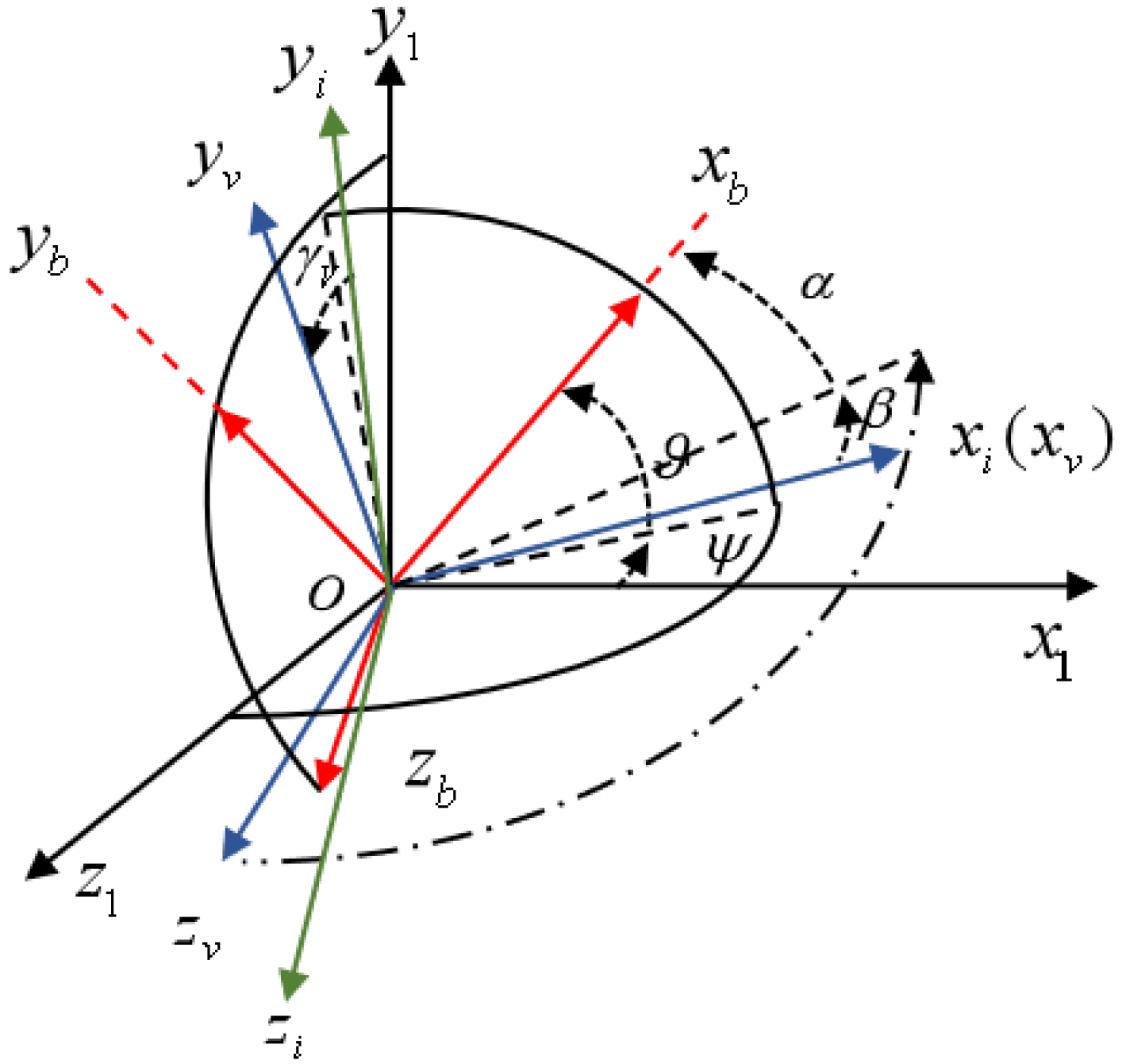
As shown in Figure 1, the inertial coordinate system $o{x}_1{y}_1{z}_1$, the body coordinate system $o{x}_b{y}_b{z}_b$, the trajectory coordinate system $o{x}_i{y}_i{z}_i$, and the velocity coordinate system $o{x}_v{y}_v{z}_v$ are presented, respectively; $\vartheta$ and $\psi$ represent the pitch angle and the yaw angle of the flight vehicle, respectively; $\alpha$ and $\beta$ are the angle of attack and the sideslip angle of the flight vehicle, respectively, and ${\gamma }_V$ represents the velocity roll angle of the flight vehicle [13].

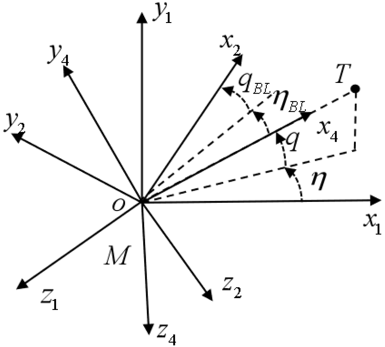
In Figure 2, the flight vehicle and a moving target are represented by M and T, respectively; $o{x}_4{y}_4{z}_4$ and $o{x}_2{y}_2{z}_2$ represent the LOS coordinate system and the body-LOS (BLOS) coordinate system, respectively; q and $\eta$ represent the LOS elevation angle and LOS azimuth angle, respectively. To simplify the problem, the BLOS elevation angle $q_{BL}$ and the BLOS azimuth angle ${\eta }_{BL}$ are introduced to represent the FOV angles in the longitudinal plane and the lateral plane, respectively. Consequently, the seeker’s FOV constraint can be formulated in terms of the BLOS angles.

The kinematic equations of the flight vehicle can be expressed as [13]:

$$\left\{\begin{array}{c}\dot{\vartheta }={\omega }_{y}sin\gamma +{\omega }_{z}cos\gamma \hfill \\ \dot{\psi }={\omega }_{y}cos\gamma sec\vartheta -{\omega }_{z}sin\gamma sec\vartheta \hfill \\ \dot{\gamma }={\omega }_x-{\omega }_{y}cos\gamma tan\vartheta +{\omega }_{z}sin\gamma tan\vartheta \hfill \\ \dot{\alpha }=\left\{\left.cos\theta [sin\vartheta cos\gamma cos(\psi -{\psi }_V)-sin\gamma sin(\psi -{\psi }_V)]-sin\theta cos\vartheta cos\gamma \right\}\right./cos\beta \hfill \\ \dot{\beta }=cos\theta [cos\gamma sin(\psi -{\psi }_V)+sin\vartheta sin\gamma cos(\psi -{\psi }_V)]-sin\theta cos\vartheta sin\gamma \hfill \\ {\dot{\gamma }}_V=(cos\alpha sin\beta sin\vartheta -sin\alpha sin\beta cos\gamma cos\vartheta +cos\beta sin\gamma cos\vartheta )/cos\theta \hfill \\ \dot{x}=Vcos\theta cos{\psi }_V\hfill \\ \dot{y}=Vsin\theta \hfill \\ \dot{z}=-Vcos\theta sin{\psi }_V\hfill \end{array}\right.$$

(1)

where $\gamma$ denotes the roll angle of the flight vehicle; $x,y,z$ represent the position of the flight vehicle; V is the magnitude of the velocity of the center of mass of the flight vehicle; $\theta$ is the angle between the velocity vector of the flight vehicle and the horizontal plane of the $o{x}_1{y}_1{z}_1$ coordinate system, and ${\psi }_V$ is the angle between the projection of the velocity vector in the horizontal plane and the $o{x}_1$ axis. They are, respectively, called the flight path angle and the heading angle.

The dynamics equations are depicted as [13]:

$$\left\{\begin{array}{c}{\dot{\omega }}_x={\displaystyle \frac{J_y-J_z}{J_x}}{\omega }_y{\omega }_z+{\displaystyle \frac{M_x}{J_x}}\hfill \\ {\dot{\omega }}_y={\displaystyle \frac{J_x-J_z}{J_y}}{\omega }_x{\omega }_z+{\displaystyle \frac{M_y}{J_y}}\hfill \\ {\dot{\omega }}_z={\displaystyle \frac{J_y-J_x}{J_z}}{\omega }_y{\omega }_x+{\displaystyle \frac{M_z}{J_z}}\hfill \\ M{\displaystyle \frac{dV}{dt}}=Pcos\alpha cos\beta -X-Mgsin\theta \hfill \\ MV{\displaystyle \frac{d\theta }{dt}}=P(sin\alpha cos{\gamma }_V+cos\alpha sin\beta sin{\gamma }_V)+Y{cos}_V-Zsin{\gamma }_V-Mgcos\theta \hfill \\ -MVcos\theta {\displaystyle \frac{d{\psi }_V}{dt}}=P(sin\alpha sin{\gamma }_V-cos\alpha sin\beta cos{\gamma }_V)+Ysin{\gamma }_V+Zcos{\gamma }_V\hfill \end{array}\right.$$

(2)

where P represents the thrust; X, Y, and Z are the components of the aerodynamic force in the directions of the respective coordinate axes of the velocity coordinate system, and they are, respectively, called the drag force, the lift force, and the side force; $M_x$, $M_y$, and $M_z$ are the components of the aerodynamic moment along the three directions of the body coordinate system, and they are, respectively, called the rolling moment, the yawing moment, and the pitching moment. The specific calculations are as follows [22]:

$$\left\{\begin{array}{c}X=QS(c_{x0}+c_x^{\alpha }|\alpha |+c_x^{\beta }\beta +c_x^{\alpha \beta }|\alpha \beta |+c_x^{{\delta }_x}|{\delta }_x|+c_x^{{\delta }_y}|{\delta }_y|+c_x^{{\delta }_z}|{\delta }_z|)\hfill \\ Y=QS(c_y^{\alpha }\alpha +c_y^{\beta }\beta +c_y^{{\delta }_z}|{\delta }_z|)\hfill \\ Z=QS(c_z^{\alpha }\alpha +c_z^{\beta }\beta +c_z^{{\delta }_y}|{\delta }_y|)\hfill \\ M_x=QSL(m_x^{\alpha }\alpha +m_x^{\beta }\beta +m_x^{{\delta }_x}{\delta }_x)\hfill \\ M_y=QSL(m_y^{\beta }\beta +m_y^{{\delta }_y}{\delta }_y)\hfill \\ M_z=QSL(m_z^{\alpha }\alpha +m_z^{{\delta }_z}{\delta }_z)\hfill \end{array}\right.$$

(3)

where $Q,S,L$ denote dynamic pressure, reference area, and reference length, respectively; M is the mass of flight vehicle; ${\omega }_x,{\omega }_y$, and ${\omega }_z$ are the components of the rotational angular velocity $\omega$ of the body coordinate system relative to the inertial coordinate system on each axis of the missile body coordinate system; $J_x,J_y$, and $J_z$ are the moments of inertia in the roll, yaw, and pitch directions, respectively; $c_{x0}, c_i^j, i=\{x, y, z\}, j = \{\alpha , \beta \}, c_x^{\alpha \beta }, c_x^n, n = \{{\delta }_x, {\delta }_y, {\delta }_z\}, c_y^{{\delta }_z}, c_z^{{\delta }_y}$ and $m_x^{\alpha }, m_x^{\beta }, m_x^{{\delta }_x}, m_y^{\beta }, m_y^{{\delta }_y}, m_z^{\alpha }, m_z^{{\delta }_z}$ represent the aerodynamic force and aerodynamic moment coefficients, respectively; ${\delta }_x, {\delta }_y, {\delta }_z$ are the aileron, rudder, and elevator deflections.

Since this paper focuses on STT flight vehicles, the roll angle is typically kept close to zero. Additionally, for the strap-down flight vehicle facing the maneuvering target, it is of utmost importance to restrict the seeker’s BLOS angle to a very small region. Under these circumstances, the relationship between the angles of $\eta , \psi , q, \vartheta$ and ${\eta }_{BL}, q_{BL}$ is given by [22]:

$$\left\{\begin{array}{c}{\eta }_{BL} = \eta - \psi \hfill \\ q_{BL} = q - \vartheta \hfill \end{array}\right.$$

(4)

Therefore, the seeker’s FOV constraint can be transformed into $|{\eta }_{BL}| \le {\sigma }_{max}, |q_{BL}| \le {\sigma }_{max}$, where ${\sigma }_{max}$ is the maximum of the FOV of the strap-down seeker.

Taking the above-mentioned factors into account, the design objective of this paper is to achieve precise guidance for moving targets while maintaining the FOV constraint and keeping the roll angle stabilized at approximately zero.

Considering the inevitable signal transmission and processing delays in practical application scenarios, a first-order link is used to represent this time delay characteristic, ensuring that the simulation environment is more in line with the operating conditions of the real world. The formula for the time delay is shown in Equation (5), where ${\delta }_i^c$ represents the signal output by the intelligent agent, and ${\delta }_i$ represents the signal actually used by the model. In addition, ${\tau }_t$ is defined as the time constant.

$${\dot{\delta }}_i = -{\displaystyle \frac{1}{{\tau }_t}}{\delta }_i + {\displaystyle \frac{1}{{\tau }_t}}{\delta }_i^c, i = x, y, z$$

(5)

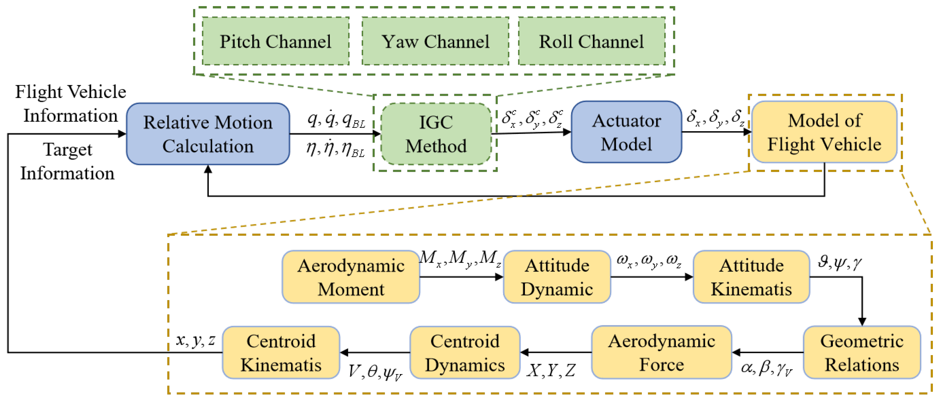
Based on the above mathematical models, the simulation process of the 6-DOF IGC model in this paper is shown in Figure 3:

Remark 1.

It should be noted that when the distance R between the flight vehicle and the target is less than a certain value $R_d$, the seeker enters the working blind area. During this period, the output information of the seeker becomes invalid, and the flight vehicle is guided by its inertial guidance system. The inertial guidance system means that after analyzing the acceleration based on hardware systems such as accelerometers, kinematic calculation methods are directly used, and no target information is required.

Remark 2.

All simulation training in this paper is conducted entirely based on the 6-DOF IGC design model.

3. The DRLIGC Method Design with FOV Constraint

In this section, the IGC algorithm for the pitch, yaw, and roll channels of the STT flight vehicle are designed independently. A DRLIGC method is put forward to control the pitch and yaw channels of the flight vehicle while adhering to the FOV constraint of the seeker. Meanwhile, the back-stepping method is employed to maintain the roll angle at approximately zero.

3.1. Twin Delayed Deep Deterministic Policy Gradient Algorithm

In this paper, the TD3 algorithm, a specific type of DRL algorithm, is harnessed for the design of the IGC method. Characterized as a data-driven intelligent algorithm, DRL refines its strategies via iterative trial-and-error processes. It is effectively applied to resolve a succession of issues within the MDP model. To leverage the capabilities of the DRL algorithm, it is imperative to cast the IGC issue into the form of an MDP model.

The MDP model includes a state space $\mathcal{S}$ that can describe the characteristics of the model, a suitable action space $\mathcal{A}$, and a comprehensive reward function $\mathcal{R}$ that takes into account the objective of the problem. At each time step t in the TD3 algorithm, the agent will select an action $a_t \in \mathcal{A}$ based on the current environmental state $s_t \in \mathcal{S}$. The environment will transition to $s_{t+1}$ according to the chosen action and provide the reward $r_t$ according to the reward function $\mathcal{R}$. 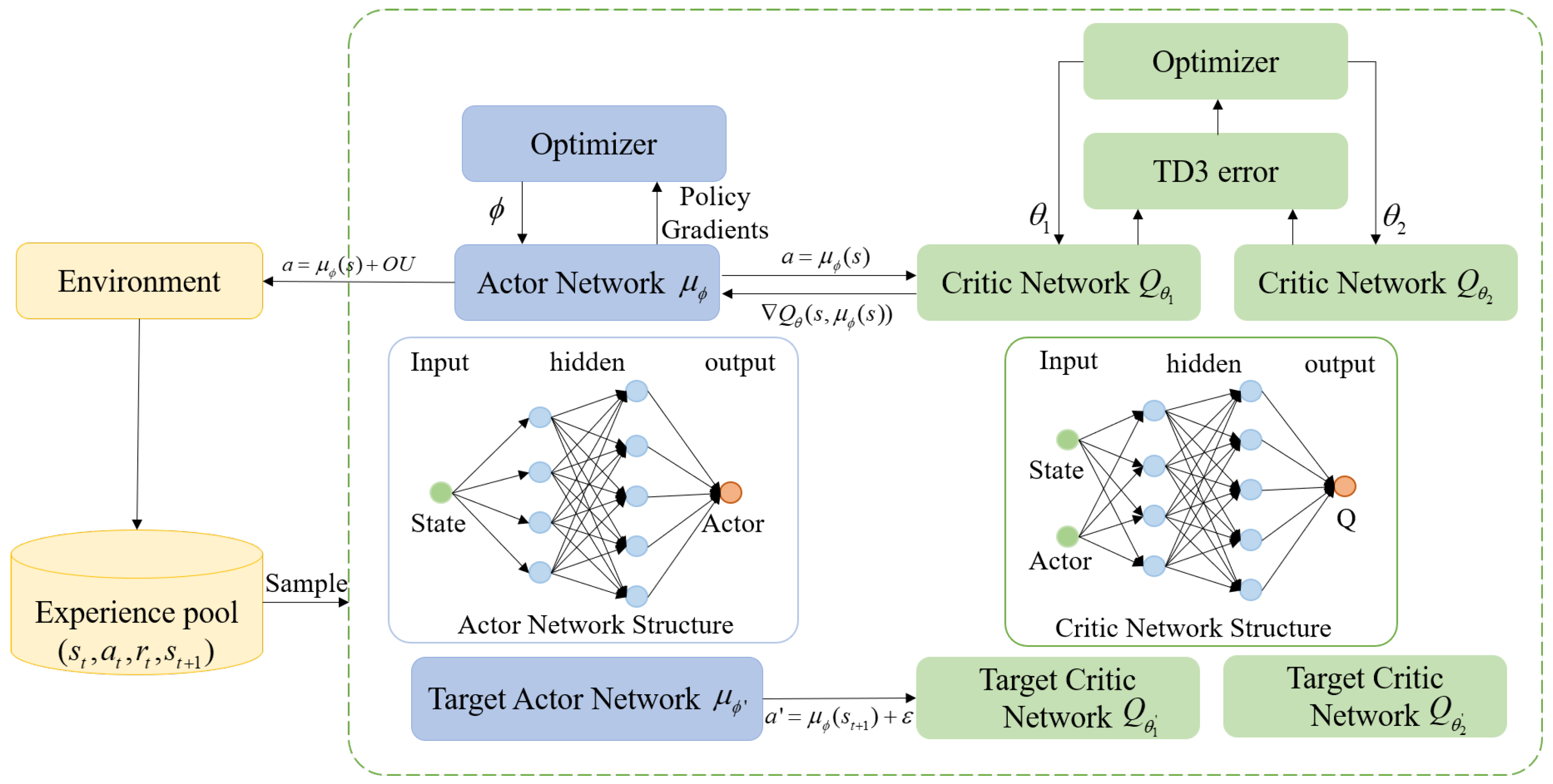Then, the agent will continuously adjust its own strategy based on the magnitude of the reward. The basic architecture of the TD3 algorithm including its network components is shown in Figure 4, where ${\mu }_{\varphi },{\mu }_{{\varphi }^{\prime }},Q_{{\theta }_i},Q_{{{\theta }_i}^{\prime }},i=1,2$ are the actor, target actor, critic network, and target critic networks, respectively; $\varphi ,{\varphi }^{\prime },{\theta }_i,{\theta }_{i^{\prime }},i=1,2$ are the corresponding network parameters, respectively.

As depicted in Figure 4, the TD3 algorithm represents a classic Actor-Critic algorithm, as noted in [34]. By incorporating two Q-networks and the target network update mechanism, it efficiently alleviates the overestimation problem that is intrinsic to policy gradient methods. This, in turn, significantly improves both the stability and the convergence rate of the algorithm. The twin delayed update mechanism ensures more stable parameter updates. Additionally, the smoothing of target networks reduces variance during the learning process. This architecture enables the TD3 algorithm to rapidly adapt and make efficient decisions in complex environments.

To address the IGC design challenge for STT flight vehicles with FOV constraints, the model ingeniously converts the FOV constraint into constraints on the BLOS angles.

This paper presents a high-precision approach IGC method that utilizes the TD3 algorithm. This method has the ability to enforce FOV constraints in the pitch and yaw channels. Through channel decomposition, the method significantly reduces the training complexity of the agent. Its objective is to directly establish a mapping from the state space to the action space obtained that the flight vehicle attains. By this way, it effectively alleviates the formidable multi-channel coupling problem inherent in the IGC issue. Figure 5 vividly depicts the information interaction between flight vehicle and environment.

3.2. MDP Model Design in Pitch and Yaw Channels

In this subsection, the IGC design of the pitch channel and the yaw channel is carried out separately. Leveraging the model-agnostic nature of the DRL algorithm, our objective is to address the strong coupling relationship that exists between the pitch and yaw channels within the IGC design model.

According to Equations (2) and (3), it can be seen that the pitch channel involves a more complex balance among lift, drag, and gravity, and the uncertainty is much higher than that of the yaw channel. Training the pitch channel first represents a more effective curriculum learning strategy. By addressing the more complex pitch control problem initially, a more stable training environment is created for the subsequent yaw training. Therefore, in this paper, the training of the intelligent agent for the pitch channel is conducted first.

When devising the DRLIGC method for the pitch channel, the corresponding IGC design model is structured as an MDP model. The entire simulation environment is grounded in the 6-DOF IGC design model introduced in Section 2. Relying on this model, the subsequent MDP model is developed.

The strap-down seeker can obtain the BLOS elevation angle $q_{BL}$ and the BLOS azimuth angle ${\eta }_{BL}$. Through further calculation, the LOS elevation angle q and the LOS azimuth angle $\eta$ can be acquired. By utilizing the observable information obtained by the strap-down seeker and the information derivable from the observable data, a suitable state space is established. A well-chosen state space has the potential to mitigate the complexity of DRL training and expedite its convergence rate.

In light of the FOV angle constraint imposed on $q_{BL}$ that the pitch channel must satisfy, state variables that can comprehensively represent this channel are carefully selected to formulate the state space, which is defined as follows:

$$s_t = (q, \dot{q}, q_{BL})$$

(6)

In order to further improve the convergence efficiency, the normalization method is employed to process the state space. Considering that the angle range within the model is $[-\pi , \pi ]$, the normalized state space is defined as follows:

$$s_t = ({\displaystyle \frac{q}{\pi }}, {\displaystyle \frac{\dot{q}}{\pi }}, {\displaystyle \frac{q_{BL}}{\pi }})$$

(7)

The action space is selected as the elevator deflection ${\delta }_z$ corresponding to the pitch channel. This choice can make full use of the data-driven characteristics of the DRL algorithm to form a direct mapping from the state space to ${\delta }_z$.

Finally, the construction of the MDP model can be finalized through careful selection of the most crucial reward function. The reward function represents the linchpin of the DRL algorithm. A well-designed reward function is capable of substantially accelerating the training of the agent and continuously fine-tuning it to conform to the specifications of the problem under consideration. This enables the agent to acquire a relatively optimal strategy.

In light of the constraints imposed on the BLOS angle within the pitch channel, as well as the ultimate necessity of attaining a high-precision target approach, and referring to the idea of achieving a quasi-parallel approach by suppressing the LOS angular rate in the classical PN guidance law, this paper determines the reward function of the pitch channel as:

$$r_y = r_{yt} + r_{{\sigma }_1} + r_{yend}$$

(8)

where $r_{yt}$ represents the immediate reward function in the pitch channel; $r_{{\sigma }_1}$ denotes the penalty term generated when $q_{BL}$ exceeds the constraint; $r_{yend}$ is the terminal reward in the pitch channel. The specific calculation method of $r_{yt}$ is formulated as:

$$r_{yt} = b_{1}exp(-{\dot{q}}^2/{\sigma }_1) + b_{2}exp(-{q_{BL}}^2/{\sigma }_2)$$

(9)

where $b_1$ and $b_2$ are the proportionality coefficients of each term, satisfying the condition that $b_1 + b_2 = 1$; ${\sigma }_1$ and ${\sigma }_2$ are the corresponding scaling coefficients. The specific calculation method of $r_{{\sigma }_1}$ is defined as:

$$r_{{\sigma }_1} = \left\{\begin{array}{c}-C_1\\ 0\end{array}\right.\begin{array}{c},if|q_{BL}| \ge {\sigma }_{max}\hfill \\ , otherwise\hfill \end{array}$$

(10)

where $C_1$ is the positive constant chosen for the penalty.

The terminal reward $r_{yend}$ is designed as:

$$r_{yend} = \left\{\begin{array}{c}{C}_2\\ 0\end{array}\right.\begin{array}{c}, R \le R_{stop}\hfill \\ , otherwise\hfill \end{array}$$

(11)

where $C_2$ is the hit reward obtained after a hit and is a selected positive constant.

When devising the reward function for the pitch channel, its content is essentially partitioned into three components. The underlying design concepts are elaborated on in the following manner:

(1)

The immediate reward function $r_{yt}$ yields the corresponding reward value at every time step. Its design intent is to minimize the LOS angular velocity $\dot{q}$. A non-linear function of the type $exp(·)$ is employed to obtain a reasonable distribution of the reward values.This approach endeavors to keep the LOS angular velocity $\dot{q}$ within a relatively narrow range to the greatest extent possible, thereby emulating the effect of the PN guidance law. Furthermore, the function $r_{{\sigma }_1}$ is crafted to maintain the BLOS angle $q_{BL}$ within a relatively small range. This serves to enhance the detection performance of the seeker. Simultaneously, this component also contributes to accelerating the convergence speed.

(2)

The FOV constraint penalty function $r_{{\sigma }_1}$ takes effect when the BLOS elevation angle $q_{BL}$ exceeds the constraint. It will impose a relatively substantial penalty value, compelling the agent to exert its utmost efforts to prevent the emergence of such a state.

(3)

The terminal reward function $r_{yend}$ is activated only upon the successful hit of the target. It will confer a relatively significant reward, informing the agent that this particular state yields greater rewards. This enables the agent to learn and gravitate towards a more optimal strategy.

Through the seamless integration of the state variables, action space, and the reward function with the established simulation model, a highly comprehensive and robust model for the pitch channel can be successfully constructed. This model can be utilized for agent training to derive the corresponding control strategy for the pitch channel, thereby forming an agent capable of directly obtaining the elevator deflection angle from the state values.

Analogously, in order to effectively tackle the FOV constraint issue within the yaw channel by means of the DRL algorithm, it is imperative to formulate the yaw channel model into an MDP model. Initially, it is crucial to establish that the FOV constraint in the yaw direction can be equivalently transformed into a constraint imposed on the LOS azimuth angle ${\eta }_{BL}$, i.e., ${\eta }_{BL} \le {\sigma }_{max}$. Based on this condition, the MDP model for the yaw channel is established.

The normalized state space constructed for the yaw channel is:

$$s_t = ({\displaystyle \frac{\eta }{\pi }}, {\displaystyle \frac{\dot{\eta }}{\pi }}, {\displaystyle \frac{{\eta }_{BL}}{\pi }})$$

(12)

Based on the characteristics of the 6-DOF model of the flight vehicle, the rudder deflection ${\delta }_y$ is chosen as the action space for the yaw channel. The reward function is crafted according to the principle of the PN guidance law. The specific form of the comprehensive reward function is designed as follows:

$$r_z = r_{zt} + r_{{\sigma }_2} + r_{zend}$$

(13)

where $r_{zt}$ represents the immediate reward function in the yaw channel; $r_{{\sigma }_2}$ denotes the penalty term generated when ${\eta }_{BL}$ exceeds the constraint; and $r_{zend}$ stands for the terminal reward in the yaw channel. The specific calculation approach of $r_{zt}$ is formulated as:

$$r_{zt}=b_{3}exp(-{\dot{\eta }}^2/{\sigma }_3)+b_{4}exp(-{{\eta }_{BL}}^2/{\sigma }_4)$$

(14)

where $b_3$ and $b_4$ are the proportionality coefficients, which meet the condition $b_3 + b_4=1$. Meanwhile, ${\sigma }_3$ and ${\sigma }_4$ are the corresponding scaling coefficients. The specific calculation method for $r_{{\sigma }_2}$ is defined as:

$$r_{{\sigma }_2} = \left\{\begin{array}{c}-C_3\\ 0\end{array}\right.\begin{array}{c}, if|{\eta }_{BL}| \ge {\sigma }_{max}\hfill \\ , otherwise\hfill \end{array}$$

(15)

where $C_3$ is the positive constant chosen for penalizing behaviors that exceed the constraints.

The terminal reward $r_{zend}$ is selected as:

$$r_{zend}=\left\{\begin{array}{c}{C}_4\\ 0\end{array}\right.\begin{array}{c}, R \le R_{stop}\hfill \\ , otherwise\hfill \end{array}$$

(16)

where $C_4$ is a selected positive constant.

Similar to the design idea of $r_y$, the comprehensive reward function $r_z$ for the yaw channel is divided into three parts: the immediate reward function $r_{zt}$, the penalty function $r_{{\sigma }_2}$ for exceeding the FOV constraint, and the terminal reward function $r_{zend}$ for target hitting. In the immediate reward function $r_{zt}$, $b_{3}exp(-{\dot{\eta }}^2/{\sigma }_3)$ aims to achieve a smaller LOS angular rate velocity, while $b_{4}exp(-{{\eta }_{BL}}^2/{\sigma }_4)$ is employed to reduce the BLOS azimuth angle. This design makes the behaviors to be constrained more explicit and accelerates the convergence rate.

Remark 3.

The training episode terminates when any of the following conditions are met: the FOV penalty reward or the terminal reward is triggered, or the relative distance between the flight vehicle and the target starts to increase. Once the episode ends, a final comprehensive reward value is obtained.

Remark 4.

Corresponding proportionality coefficients are used to strike a balance between target engagement and constraint satisfaction. As a result, the sum of these proportionality coefficients in the corresponding rewards must equal to one.

Remark 5.

The scaling coefficients are utilized to adjust the magnitudes of the corresponding elements. They have a pronounced impact on the convergence of DRL training. Moreover, within the function $exp(·)$, the scaling coefficients contribute to determining the magnitudes of the optimal values of the corresponding variables.

Remark 6.

Differences in training step sizes lead to varying frequencies of obtaining immediate rewards. This variation directly impacts the influence exerted by the remaining components of the comprehensive reward function on the strategy formulation. As a result, different hyperparameters are required.

3.3. DRLIGC Method

In the DRLIGC method utilizing the TD3 algorithm, the training process commences with the independent training of the pitch channel. During this initial stage, the acceleration command of the yaw channel is directly determined according to the PN guidance law. Meanwhile, the roll angle and angular velocity of the roll channel are both set to zero. Under these conditions, the yaw channel achieves relatively high approach accuracy, which provides a stable environment for the separate training of the pitch channel. After the training phase, a highly effective engagement agent for the pitch channel is successfully obtained. The PN guidance law applied to the yaw channel is presented as follows:

$$a_z = -NV\dot{\eta }$$

(17)

where N is the proportionality coefficient.

Once the pitch-channel agent is acquired, the yaw channel is switched to normal computation mode, and the yaw-channel agent is introduced into the training process. At this stage, the training effort is concentrated exclusively on the yaw-channel agent. Through this targeted training, a yaw-channel agent that disregards the roll factor can be obtained. By integrating this yaw-channel agent with the previously obtained pitch-channel agent, a DRLIGC method that does not take the roll factors into account can be developed. This approach streamlines the system design and potentially enhances the computational efficiency while maintaining an acceptable level of performance for the engagement task. The specific training process of the DRLIGC method is illustrated in Figure 6, with the algorithm for the pitch channel shown in Figure 7.

The DRLIGC procedure for the yaw channel is similar to that of the pitch channel, so it will not be repeated here. Through the process described above, the DRLIGC method that excludes the consideration of the roll channel is obtained. Regarding the roll channel, this paper adopts an adaptive control law based on the back-stepping method to carry out roll angle control. The model of the roll channel is as follows [13]:

$$\left\{\begin{array}{c}\dot{\gamma } = -{\omega }_{y}cos\gamma tan\vartheta + {\omega }_{z}sin\gamma tan\vartheta + {\omega }_x\hfill \\ {\dot{\omega }}_x={\displaystyle \frac{J_y-J_z}{J_x}}{\omega }_y{\omega }_z + {\displaystyle \frac{QSL{m}_x^{{\delta }_x}}{J_x}}{\delta }_x+d_{{\omega }_x}\hfill \end{array}\right.$$

(18)

where $d_{{\omega }_x}$ denotes the disturbance term, caused by aerodynamic moments.

Select the state variables as $x_1=\gamma ,x_2={\omega }_x$ and control input as $u={\delta }_x$, the roll channel model can be transformed into:

$$\left\{\begin{array}{c}{\dot{x}}_1=f_1(\vartheta ,{\omega }_y,{\omega }_x)+x_2\hfill \\ {\dot{x}}_2=f_2({\omega }_y,{\omega }_z)+g_{1}u+d_2\hfill \end{array}\right.$$

(19)

where

$$\left\{\begin{array}{c}{f}_1(\vartheta ,{\omega }_y,{\omega }_z)=-{\omega }_{y}cos\gamma tan\vartheta +{\omega }_{z}sin\gamma tan\vartheta \hfill \\ f_2({\omega }_y,{\omega }_z)=(J_y-J_z){\omega }_y{\omega }_z/J_x\hfill \\ g_1=QSL{m}_x^{{\delta }_x}/J_x\hfill \\ d_2=d_{{\omega }_x}\hfill \end{array}\right.$$

(20)

The roll channel IGC method presented in [13] is employed in this study and is defined as:

$$\left\{\begin{array}{c}{s}_1 = x_1\hfill \\ x_{2d} = -k_1{s}_1-f_1(\vartheta ,{\omega }_y,{\omega }_z)\hfill \\ \tau {\dot{x}}_{2c} + x_{2c} = x_{2d}, x_{2c}\left(0\right) = x_{2d}\left(0\right)\hfill \\ s_2 = x_2 - x_{2c}\hfill \\ u = g_1^{-1}(-f_2-\widehat{\rho }{s}_2+{\dot{x}}_{2d}-s_1-k_2{s}_2)\hfill \\ \dot{\widehat{\rho }}=\lambda ({s_2}^2+\sigma \widehat{\rho })\hfill \end{array}\right.$$

(21)

where $k_1, k_2, \lambda , \sigma$ represent the designed parameters, where $\widehat{\rho }$ stands for the estimation of $\rho$. Here, $\rho$ denotes the unknown upper bound of $d_2$, satisfying the condition $|d_2| \le \rho$.The proof of the stability of the roll IGC method can be retrieved in [13]. By utilizing the above-mentioned roll IGC method, the objective of keeping the roll angle controlled around zero can be realized.

During the simulation process, when $R \ge R_d$, the flight vehicle is guided using the DRLIGC algorithm proposed in this paper. When $R < R_d$, it switches to inertial guidance. At this time, it can be regarded as an unguided section. The acceleration and its direction are provided by the acceleration measurement components inside the flight vehicle, and the subsequent motion trajectory is calculated through kinematic integration.

4. Numerical Simulation Analysis

In this section, a comprehensive account of the training scenarios, hyperparameters, and network parameters associated with the DRLIGC method is provided. Moreover, numerical simulations are carried out to verify the viability and effectiveness of this method.

4.1. DRLIGC Training Settings

To cultivate robust agents for the pitch and yaw channels within the DRLIGC method, variables are randomly initialized across a multitude of scenarios. The specific adjustments are comprehensively detailed in

Table 1. Initialization range for random scenarios.

Parameter	Min	Max	Parameter	Min	Max
$X_{T0}$	2800	3000	$V_{xT}$	30	40
$V_{yT}$	30	40	$V_{zT}$	15	25
${\sigma }_{max}$	7		$R_{stop}$	30

, from which the corresponding parameters are selected.

The flight vehicle is initially positioned at (0, 200, 0) m, boasting an initial velocity of 400 m/s. The initial values of both its attitude angles and angular velocities are set to 0. The target starts at the position ($X_{T0}$, 0, 0) m, with an initial velocity of ($V_{xT}$, $V_{yT}$, $V_{zT}$). The chosen maneuver acceleration is (4, 0, 2) m/${\mathrm{s}}^2$. The FOV constraint size ${\sigma }_{max}$ of the flight vehicle’s seeker is set to $7^{°}$. Taking into account the detection frequency limitation of the seeker, the training step size is set at 0.05 s, while the simulation step size is fixed at 0.01 s. The time constant ${\tau }_t$ is randomly selected between 0.01 and 0.2. Given the simulation step size of 0.01 s and considering the velocities of the flight vehicle and the target, the value of $R_{stop}$ is set to 30 m.

The network architectures of the pitch channel and the yaw channel are identical.

Table 2. Network layer size.

Layer	Actor Network	Critic Network
Input layer	3 (the dimension of s)	4 (the dimension of s+ the dimension of a)
Hidden Layer 1	64	64
Hidden Layer 2	128	128
Hidden Layer 3	128	128
Hidden Layer 4	64	64
Output Layer	1 (the dimension of a)	1 (the dimension of a)

details the specific number of layers and nodes in the Actor and Critic networks. For the Actor network, the activation layer employs the tanh function. Moreover, the target network shares the same architecture as the corresponding network.

The settings of the relevant hyperparameters in the reward function and the DRL algorithm are elaborated in

Table 3. Hyper-parameters in shaping the reward function.

${\mathit{b}}_1$	${\mathit{b}}_2$	${\mathit{b}}_3$	${\mathit{b}}_4$	${\mathit{\sigma }}_1$	${\mathit{\sigma }}_2$	${\mathit{\sigma }}_3$	${\mathit{\sigma }}_4$	${\mathit{C}}_1$	${\mathit{C}}_2$	${\mathit{C}}_3$	${\mathit{C}}_4$
0.8	0.2	0.8	0.2	0.04	0.04	0.04	0.04	50	50	50	50

and

Table 4. Algorithm hyperparameter settings.

Parameter	Value	Parameter	Value
Discount factor	0.99	$L_2$ regularization constant	$5\times {10}^{-4}$
Experience pool size	${10}^6$	Upper bound of the gradient	1
Sample size	256	Average attraction constant	0.7
Actor learning rate	$1\times {10}^{-4}$	Policy frequency	2
Critic learning rate	$1\times {10}^{-4}$	Soft update rate $\kappa$	$5\times {10}^{-3}$
Policy noise variance	0.1	Ornstein–Uhlenbeck (OU) noise	0.2
Maximum noise value	0.1	Type of optimization algorithm	Adam

, respectively.

Table 5. The aerodynamic characteristics of the flight vehicle.

Name	Value	Name	Value	Name	Value
M	1200	$m_y^{\beta }$	−27.31	$c_x^{{\delta }_x}$	0.05
P	0	$m_y^{{\delta }_y}$	−26.57	$c_x^{{\delta }_y}$	0.07
$J_x$	100	$m_x^{{\delta }_x}$	2.12	$c_x^{{\delta }_z}$	0.06
$J_y$	5700	$m_x^{\alpha }$	0.46	$c_y^{\alpha }$	57.16
$J_z$	5600	$m_x^{\beta }$	−0.37	$c_y^{{\delta }_z}$	5.74
S	0.42	$c_{x0}$	0.32	$c_y^{\beta }$	−0.08
L	0.68	$c_x^{\alpha }$	0.21	$c_z^{\beta }$	−56.31
$m_z^{\alpha }$	−28.16	$c_x^{\beta }$	0.19	$c_z^{{\delta }_y}$	−5.62
$m_z^{{\delta }_z}$	−27.92	$c_x^{\alpha \beta }$	25.38	$c_z^{\alpha }$	0.09

provides the aerodynamic characteristics of the flight vehicle, which are derived from the data reported in [22]. Meanwhile,

Table 6. The parameter of the roll channel.

${\mathit{k}}_1$	${\mathit{k}}_2$	$\mathit{\tau }$	$\mathit{\lambda }$	$\mathit{\sigma }$
60	60	0.01	0.1	0.1

provides a detailed breakdown of the relevant parameters in Equation (21).

4.2. DRLIGC Method Training

Based on the scenario settings and relevant parameter configurations in Section 4.1, the DRLIGC method is applied to carry out DRL training for the pitch channel and the yaw channel separately. The training results of the pitch channel and yaw channel are presented in Figure 8 and Figure 9, respectively.

In Figure 8 and Figure 9, the average reward is calculated as the mean of the episode rewards from the adjacent 30 episodes. This metric serves as an indicator of the current agent’s stability.

We conducted an in-depth analysis of the curve in Figure 8. The entire training process for the pitch channel spans 1500 episodes. Approximately at the 200th episode, the reward reaches its peak. This suggests that the agent has discovered a strategy that can successfully approach the target within the constraints of the FOV. Around the 700th episode, the reward value begins to stabilize. By the 1300th episode, convergence is attained, signifying that a relatively superior strategy has been formulated. It can be seen from Figure 9 that the reward value hits its peak multiple consecutive times around the 400th episode for the yaw channel. This implies that, through continuous optimization, the strategy enables successful approaches in both channels. Convergence is achieved after the 1300th episode. When running on an Intel(R) Core(TM) i7-1065G7 CPU using the MATLAB R2023b Reinforcement Learning Toolbox, the total off-line training time for the pitch and yaw channels amounts to 7.3 h and 6.8 h, respectively.

An attempt was made to integrate the pitch and yaw channels into a single agent. This unified agent was designed with six inputs and two outputs, aiming to concurrently determine the rudder and elevator deflections of the flight vehicle. However, it was found that the coupling between the pitch and yaw channels was excessively severe. This high-level coupling made it extremely difficult for the agent to be trained and to converge. As a result, it was a great challenge to realize a successful approach. In contrast, the DRLIGC method proposed in this paper showcases certain advantages. It can effectively achieve target engagement, providing a more feasible and efficient solution for the engagement task.

4.3. Monte Carlo Simulation

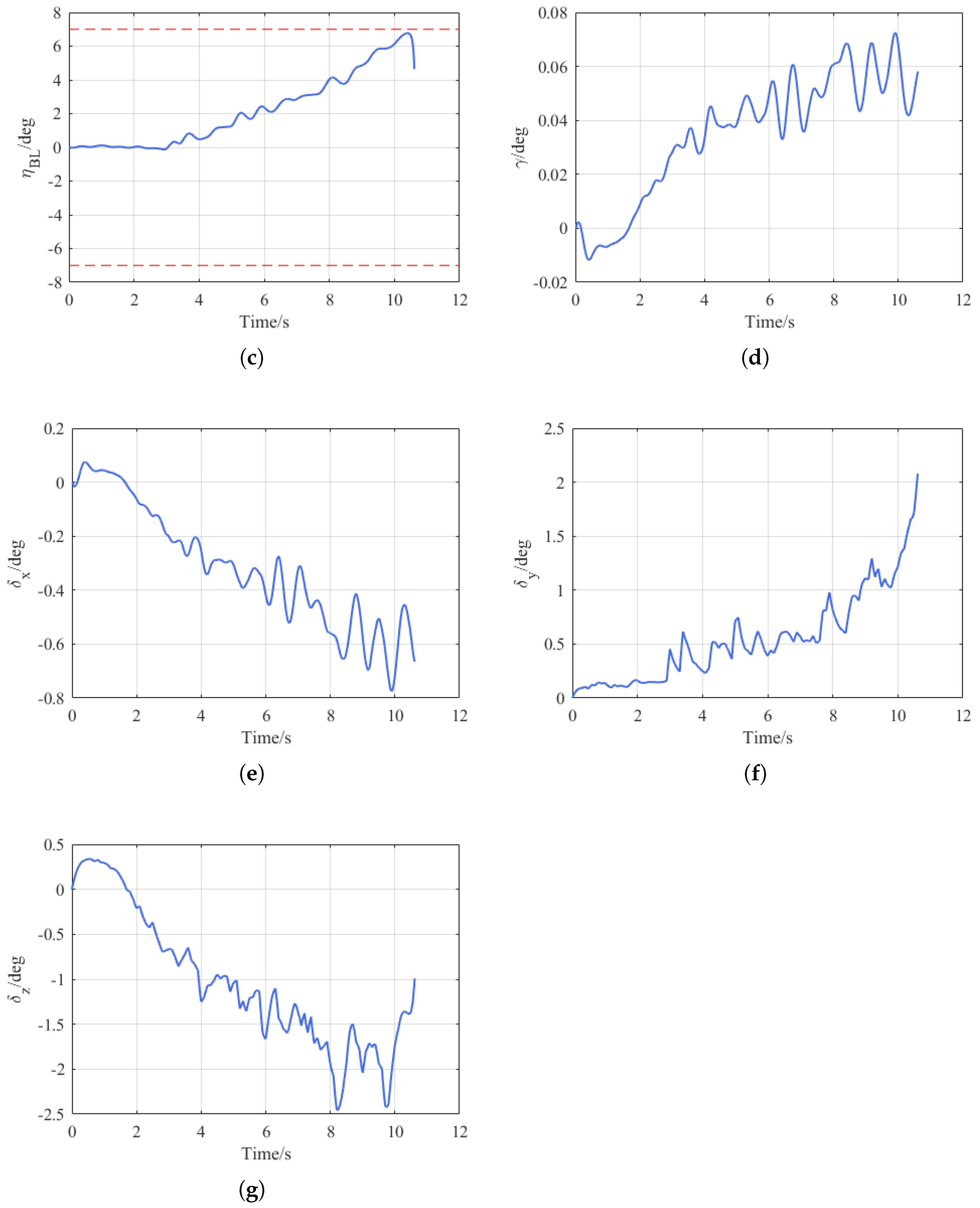
To validate the feasibility and robustness of the DRLIGC method put forward in this paper, a Monte Carlo simulation experiment encompassing 500 episodes was carried out. In this MC simulation experiment, scenarios were randomly chosen from those elaborated in Table 1. The specific simulation results are presented in Figure 10.

In Figure 10a, the flight trajectories of the flight vehicle and the target are depicted. The solid line denotes the flight vehicle’s trajectory, while the dotted line represents that of the target. Evidently, the flight vehicle’s flight path appears normal. Figure 10b,c, respectively, exhibit the curves of the flight vehicle’s BLOS elevation angle $q_{BL}$ and azimuth angle ${\eta }_{BL}$. When combined with Figure 11, it can be clearly observed that throughout the entire guidance process, both angles are within the FOV constraint range. Figure 10d presents the roll angle curve of the flight vehicle. It is apparent that the roll angle remains close to zero with a relatively small amplitude, thus satisfying the design requirements. Figure 10e–g, respectively, display the aileron, rudder, and elevator deflections of the flight vehicle. Figure 11c represents the miss distance. Through statistical analysis, it is found that the mean value of the miss distance amounts to 0.6731 m, and the variance is 0.0699.

To study the impact of noise on the performance of the DRLIGC method proposed in this paper, a set of simulations is conducted while taking into account the influence of noise on the observed values. Random Gaussian noise with a mean value of 0° and a variance of 0.2 was added to $(q,q_{BL},\eta ,{\eta }_{BL})$. The simulation results are shown in Figure 12. After adding the noise, the FOV constraint can still be satisfied and the target can be successfully hit, with the miss distance being 0.70 m. The above simulation experiments further verified the feasibility of the DRLIGC method.

4.4. Comparison Study

To further substantiate the superiority of the proposed DRLIGC method, a comparative analysis is carried out in this subsection. The comparative algorithm employs the 3D IBLF-IGC algorithm presented in [22]. The specific details of the IBLF-IGC algorithm are presented as follows:

$$\left\{\begin{array}{c}{s}_1=x_1\hfill \\ x_{2d}=-k_Q({\widehat{D}}_1{\lambda }_1+1)s_1-k_1{s}_1\hfill \\ {\tau }_2{\dot{x}}_{2c}+x_{2c}=x_{2d}\hfill \\ s_2=x_2-x_{2c}\hfill \\ x_{3d}^{\#}=g_2^{-1}\left(t\right)(-{\widehat{D}}_2{\lambda }_2{s}_2-k_2{s}_2-f_2(x_2,x_3^{\#})+{\dot{x}}_{2c})\hfill \\ {\tau }_3{\dot{x}}_{3c}^{\#}+x_{3c}^{\#}=x_{3d}^{\#}\hfill \\ s_3^{\#}=x_3^{\#}-x_{3c}^{\#},s_3=x_3-{\left[\begin{array}{cc}0& {x_{3c}^{\#}}^T\end{array}\right]}^T\hfill \\ x_{4d}=g_3^{-1}(\vartheta ,x_3)(-{\widehat{D}}_3{\lambda }_3{s}_3-k_3{s}_3-f_3\left(x_3\right)+{\left[\begin{array}{cc}0& {{\dot{x}}_{3c}^{\#}}^T\end{array}\right]}^T)\hfill \\ {\tau }_4{\dot{x}}_{4c}+x_{4c}=x_{4d}\hfill \\ s_4=x_4-x_{4c}\hfill \\ u=g_4^{-1}\left(t\right)(-{\widehat{D}}_4{\lambda }_4{s}_4-k_4{s}_4-f_4(x_3^{\#},x_4)+{\dot{x}}_{4c})\hfill \end{array}\right.$$

(22)

where $$\begin{gathered} x_1={\left[\begin{array}{cc}{\eta }_{BL}& q_{BL}\end{array}\right]}^T, x_2={\left[\begin{array}{cc}\dot{\eta }& \dot{q}\end{array}\right]}^T, x_3^{\#}={\left[\begin{array}{cc}\beta & \alpha \end{array}\right]}^T,x_3={\left[\begin{array}{ccc}\gamma & \beta & \alpha \end{array}\right]}^T, \\ {x}_4={\left[\begin{array}{ccc}{\omega }_x& {\omega }_y& {\omega }_z\end{array}\right]}^T, u={\left[\begin{array}{ccc}{\delta }_x& {\delta }_y& {\delta }_z\end{array}\right]}^T, r=Rsinq, \\ {f}_2\left(x_2{x}_3^{\#}\right)=-\left[\begin{array}{c}{\displaystyle \frac{2\dot{R}\dot{\eta }cosq}{r}}-{\displaystyle \frac{2R\dot{\eta }\dot{q}sinq}{r}}+Pcos\alpha sin\beta \\ {\displaystyle \frac{2\dot{R}\dot{q}}{R}}+{\displaystyle \frac{{\dot{\eta }}^{2}rsin\epsilon }{R}}+{\displaystyle \frac{Psin\alpha }{mR}}\end{array}\right], g_2\left(t\right)=\left[\begin{array}{cc}{\displaystyle \frac{QS{c}_z^{\beta }}{mr}}& 0\\ 0& -{\displaystyle \frac{QS{c}_y^{\alpha }}{mR}}\end{array}\right], \\ {f}_3\left(x_3^{\#}\right)=\left[\begin{array}{c}0\\ {\displaystyle \frac{1}{mV}}(QS{c}_z^{\beta }\beta -Pcos\alpha sin\beta )\\ -{\displaystyle \frac{1}{mVcos\beta }}(Psin\alpha +QS{c}_y^{\alpha }\alpha )\end{array}\right], f_4(x_3^{\#},x_4)=\left[\begin{array}{c}{\displaystyle \frac{J_z-J_y}{J_x}}{\omega }_y{\omega }_z\\ {\displaystyle \frac{1}{J_y}}QSL{m}_y^{\beta }\beta +{\displaystyle \frac{J_x-J_z}{J_y}}{\omega }_x{\omega }_z\\ {\displaystyle \frac{1}{J_z}}QSL{m}_z^{\alpha }\alpha +{\displaystyle \frac{J_y-J_x}{J_z}}{\omega }_x{\omega }_y\end{array}\right], \\ {g}_3(\vartheta ,x_3)=\left[\begin{array}{ccc}1& -tan\vartheta cos\gamma & tan\vartheta sin\gamma \\ sin\alpha & cos\alpha & 0\\ -tan\beta cos\alpha & sin\alpha tan\beta & 1\end{array}\right], k_Q=\left[\begin{array}{cc}{\displaystyle \frac{{\sigma }_{max}^2}{{\sigma }_{max}^2-x_{11}^2}}& 0\\ 0& {\displaystyle \frac{{\sigma }_{max}^2}{{\sigma }_{max}^2-x_{12}^2}}\end{array}\right], \\ {g}_4\left(t\right)=\left[\begin{array}{ccc}{\displaystyle \frac{1}{J_x}}QSL{m}_x^{{\delta }_x}& 0& 0\\ 0& {\displaystyle \frac{1}{J_y}}QSL{m}_y^{{\delta }_y}& 0\\ 0& 0& {\displaystyle \frac{1}{J_z}}QSL{m}_z^{{\delta }_z}\end{array}\right], \left\{\begin{array}{c}{\dot{\widehat{D}}}_1={\lambda }_1{s_1}^T{k}_Q^2{s}_1-{\mu }_1{\widehat{D}}_1\\ {\dot{\widehat{D}}}_2={\lambda }_2{s_2}^T{s}_2-{\mu }_2{\widehat{D}}_2\\ {\dot{\widehat{D}}}_3={\lambda }_3{s_3}^T{s}_3-{\mu }_3{\widehat{D}}_3\\ {\dot{\widehat{D}}}_4={\lambda }_4{s_4}^T{s}_4-{\mu }_4{\widehat{D}}_4\end{array}\right.. \end{gathered}$$

The design parameters of the IBLF-IGC algorithm are given by $k_1=diag(0.1,0.1)$, $k_2=diag(3,3),k_3=diag(60,3,3).k_4=diag(60,20,20),{\tau }_2=diag(0.1,0.1)$, ${\tau }_3=diag(0.1,0.1),{\tau }_4=diag(0.05,0.05,0.05),{\lambda }_i,{\mu }_i(i=1,2,3,4)=0.1$.

The QLF-IGC algorithm, as elaborated on in [22], is employed to illustrate the indispensability of FOV constraints within the present scenario. This algorithm bears resemblance to the IBLF-IGC algorithm yet incorporates the following modifications:

$$\left\{\begin{array}{c}{x}_{2d}=-{\widehat{D}}_1{\lambda }_1{s}_1-k_1{s}_1\hfill \\ {\dot{\widehat{D}}}_1={\lambda }_1{s}_1^T{s}_1-k_{12}{\widehat{D}}_1\hfill \end{array}\right.$$

(23)

In order to further validate the robustness of the algorithm put forward in this paper, within the comparative simulation scenarios, the target maneuver is intensified to a certain degree. The specific scenarios are presented in

Table 7. Simulation scenario of the comparative study.

${\mathit{X}}_{\mathit{T}0}$	${\mathit{V}}_{\mathbf{xT}}$	${\mathit{V}}_{\mathbf{yT}}$	${\mathit{V}}_{\mathbf{zT}}$	${\mathit{\sigma }}_{\mathbf{max}}$	${\mathit{a}}_{\mathbf{xT}}$	${\mathit{a}}_{\mathbf{yT}}$	${\mathit{a}}_{\mathbf{zT}}$	$\mathit{\tau }$
3000	40	30	20	7	4	2	3	0.1

.

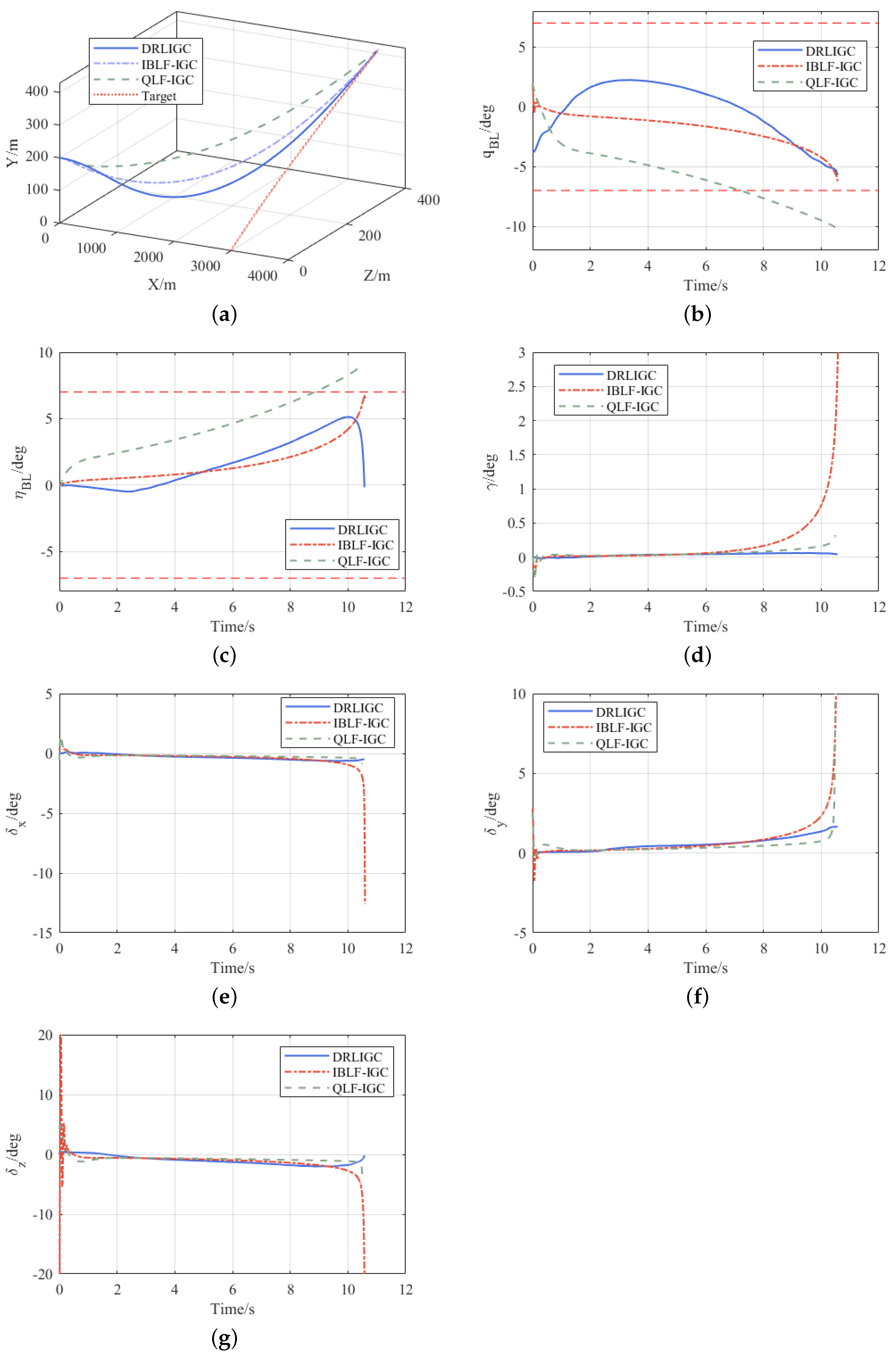
The results of the comparative simulation are shown in Figure 13.

As illustrated in Figure 13, the results of the comparative simulation reveal that the DRLIGC method, along with the IBLF-IGC and QLF-IGC algorithms, all accomplished successful target approach. Specifically, the miss distances were measured at 0.76 m for the DRLIGC method, 1.18 m for the IBLF-IGC algorithm, and 0.97 m for the QLF-IGC algorithm. Significantly, both the DRLIGC and IBLF-IGC algorithms strictly complied with the FOV constraint conditions. However, the QLF-IGC algorithm failed to meet these constraints, which powerfully emphasizes the indispensability of integrating FOV constraints within the current scenario. Furthermore, during the approach phase, the IBLF-IGC algorithm prematurely encountered divergence problems. Such issues have the potential to severely undermine the guidance effectiveness in particular circumstances, thus highlighting its relatively lower stability. In marked contrast, the DRLIGC method demonstrated outstanding stability, standing out as a more reliable and robust solution in comparison to the other algorithms under study.

Within the identical scenario described in Section 4.3, 500 iterations of MC simulations are carried out for the IBLF-IGC algorithm. The obtained miss distance yielded an average value of 0.9715 m and a variance of 0.1273. This clearly indicates that the DRLIGC algorithm proposed in this study not only showcases higher approach accuracy but also exhibits superior overall performance, highlighting its effectiveness and reliability in comparison to other approaches in the context of target engagement tasks.

Remark 7.

As the approach phase nears its end, divergence becomes evident in several simulation curves. This is because as the flight vehicle approaches and passes the target, it causes the angular velocity of the line of sight to diverge. This divergence leads to a sharp increase in some physical quantities. At this moment, the relative distance between the flight vehicle and the target has become close enough, enabling a successful approach.

5. Conclusions

In addressing the IGC design challenge for STT flight vehicles in 3D scenarios, this paper proposes a novel DRLIGC method, which takes into account both the FOV constraint of the strap-down seeker and approach accuracy.

We employ a channel-separated approach to decompose the design model into three distinct channels: pitch, yaw, and roll. Specifically, the roll channel is stabilized using the back-stepping method, ensuring its stability and smooth operation, while the pitch and yaw channels are designed with the DRLIGC method based on the TD3 algorithm.

A comprehensive reward function considering the FOV constraint conditions and approach accuracy is designed. This function effectively capitalizes on the model-free advantage of the DRL algorithm. As a result, it can directly map the designed state space to the deflection angle of the corresponding channel, enabling more accurate and efficient control. Simulation results verify the effectiveness and superiority of the proposed method and reflect the broad potential of the DRL algorithm in the field of IGC design.