Deep Learning-Based Prediction of Commercial Aircraft Noise: A CNN–Transformer Hybrid Model Versus Support Vector Regression and Multi-Layer Perceptron

Abstract

The rapid growth of the aviation industry and increasing air traffic demand more careful attention to environmental concerns. Among these, aircraft noise is considered one of the main sources of environmental noise, especially after land-based transportation. The World Health Organization highlights noise pollution as the second-most important environmental factor after air pollution, with serious consequences for public health. Long-term exposure to high noise levels has been linked to problems such as cardiovascular disease and sleep disruption. In response, ICAO has introduced stricter standards especially in Annex 16, Volume I requiring aircraft to meet tighter noise limits. This study focuses on estimating the noise levels of Airbus and Boeing aircraft during approach, lateral, and flyover phases. The models use parameters such as maximum take-off and landing weights, engine thrust, and bypass ratio. Three approaches are compared: Support vector regression (SVR), a classical machine learning method, multi-layer perceptron(MLP), and a CNN–Transformer hybrid model, which combines deep learning and attention-based techniques. Their predictive performances were evaluated using MSE, RMSE, MAE, MAPE, and R². The CNN–Transformer showed better results in all metrics. At the flyover point, it reached an R² of 0.981, compared to 0.898 for SVR and 0.919 for MLP. At the lateral point, its MAE dropped to 0.58, while SVR had 1.64 and MLP 1.17. The attention-based model found patterns that the traditional one missed. It gave better results in several cases. Apart from this, some technologies used to reduce noise may also help save fuel and increase energy efficiency. For example, engines with a high bypass ratio can lower both noise and emissions. These kinds of solutions connect performance with environmental benefits. These insights could be useful for those involved in airport planning, aircraft engine design, or regulatory planning.

1. Introduction

The commercial aviation sector is one of the fastest growing in the world. It is highly resilient to outside shocks. Despite the effects of war, global disease, and the financial crisis, the global annual air traffic rapidly grows every year between 1988 and 2018 [1]. According to Airbus’s 2022 worldwide market prediction, air traffic will increase to 2019 levels between 2023 and 2025, despite a major decrease in global air traffic volume since 2020 as a consequence of COVID-19 [2]. Air passenger traffic and freight traffic will increase by 3.6% and 3.2%, respectively, by 2041. From 2020 to 2041, aircraft operating worldwide will increase from 22,880 to 46,930. A total of 39,490 new aircraft are estimated to be needed by the world civil aviation sector, of which 24,050 would be required to satisfy the rising demand for air travel. Rising air traffic activities means that it will cause environmental and noise pollution [2]. The emergence of stricter regulations regarding noise pollution in the aviation industry has made it necessary to use low-noise technologies in aircraft. Although innovations in noise reduction have partially reduced noise, this issue is considered a significant obstacle in the short term. In particular, the expansion of airports close to city centers poses a challenge for the aviation sector, which tends to grow by 5% annually [3]. The World Health Organization states that noise pollution is the biggest factor affecting the environment after air pollution [4]. The biggest traffic noise after road and railway traffic noise is aviation noise [5,6]. Aviation noise is defined as the noise generated by the engine, landing gear, fuselage, the flight control surfaces such as flaps, slats, elevators, rudder and other components of the aircraft during flight [7]. The greatest environmental impacts of aviation are emissions and noise, and these impacts are controlled by ICAO Annex 16 regulations. Although quieter aircraft and low-noise technologies are being adopted in aviation systems, noise is still seen as a major problem for people living close to airports. For this reason, it has been emphasized that the noise level emitted by aircraft should be reduced as much as possible and especially below 45 dB [8]. With the addition of innovative technologies to aircraft systems in the last fifty years, fuel consumption and hydrocarbon (HC) and carbon monoxide (CO) emissions have been reduced by 70% and 90%, respectively, while a 50% decrease in noise levels has been observed [9]. When the noise-producing mechanisms in gas turbine engines are examined, it has been determined that rotating components such as propellers, fans, compressors and turbines are the main noise sources. In addition, the sudden encounter of high-speed jet gases with cold air can also cause serious noise. The problem can be solved by reducing the jet exit speed or by increasing the mixing speed of hot gases with cold air. Since jet noise is proportional to the eighth power of the jet speed, even a small reduction in jet speed can significantly reduce the noise level [10]. ACARE aims to reduce commercial aircraft noise in Europe by 65% and overall sound pressure levels (OASPLs) by 12 dB by 2050, compared to the levels in 2000 [11]. The ICAO aims to reduce the number of people exposed to high noise levels, which can lead to health issues such as cardiovascular disease. Various noise reduction techniques have been applied to aircraft and their subsystems; two primary methods have been implemented at the aircraft level by reducing noise sources and at the operational level by minimizing the perceived impact on the ground. For example, one technique involves retrofitting engines with acoustic linings, while another focuses on increasing the bypass ratio. Another strategy is to implement flight techniques that produce less noise. Innovations aimed at reducing aircraft noise have led to noise levels dropping from approximately 100 EPNdB to 90 EPNdB between 1965 and 2015. In this context, A320 aircraft, classified as medium category, has noise levels around 93–94 decibels, whereas the A320neo causes noise levels below 90 decibels [12]. There are various semi-empirical methods to estimate aircraft noise within comprehensive models, including ANP created by EUROCONTROL, ANOPP2 by NASA, and PANAM by DLR [13].

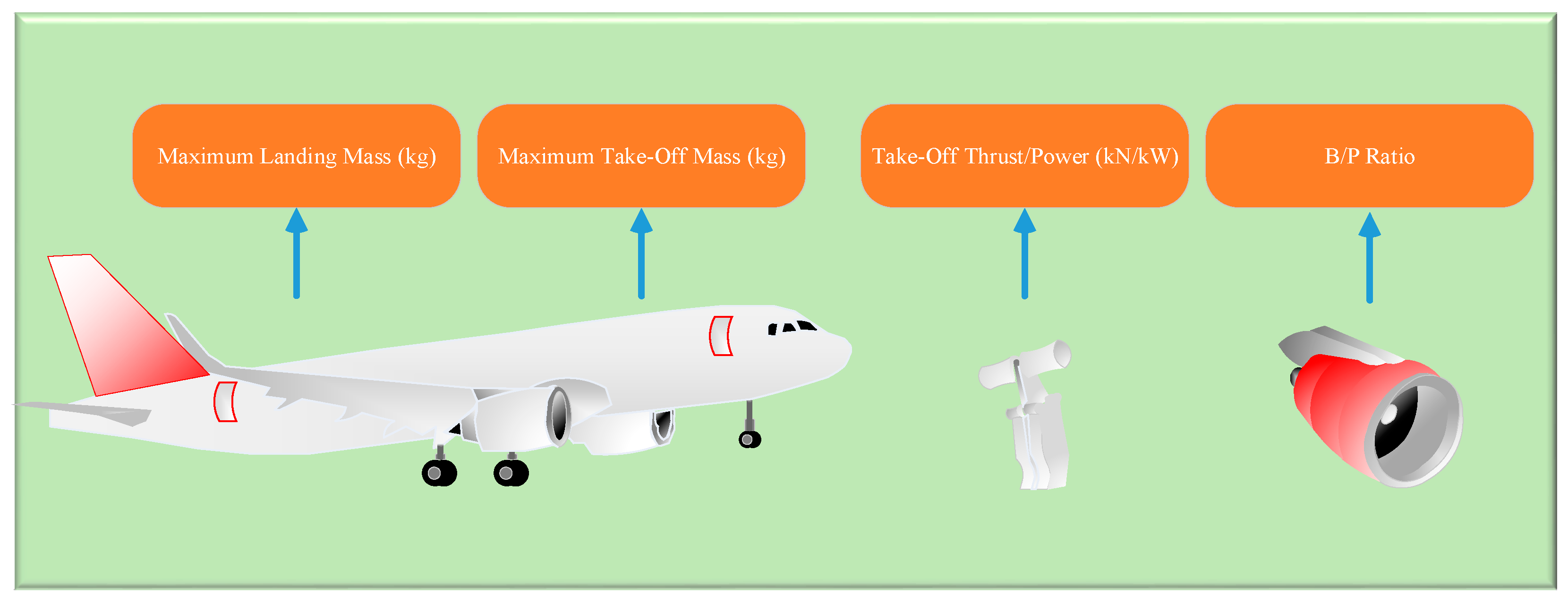
This study introduces a CNN–Transformer hybrid model for predicting aircraft noise using ICAO-certified EPNL data derived from real aircraft types’ MLM, MTOM, take-off thrust, and bypass ratio. The framework bridges the gap between regulatory datasets and modern predictive modeling, offering a transferable baseline applicable to aeroacoustic assessment and certification analysis.

The study focuses on estimating aircraft noise levels at the approach, flyover, and lateral points using three predictive approaches: SVR, MLP, and a CNN–Transformer hybrid model.

Although sound pressure level (SPL) and overall sound pressure level (OASPL) are commonly used in aeroacoustic analyses, this study primarily employed the Effective Perceived Noise Level (EPNL), which is the official metric used in ICAO Annex 16 certification procedures. Unlike SPL, which quantifies the instantaneous acoustic pressure, EPNL integrates the frequency and duration weighting of human auditory perception. Therefore, EPNL provides a standardized and perceptually relevant measure for comparing certified aircraft noise levels.

Related Work

Previous studies have investigated both theoretical and data-driven methods for predicting or mitigating aircraft noise.

Ozkaya et al. [14] performed the design optimization of acoustic coatings in the bypass duct of turbofan engines and presented an optimization strategy for noise reduction. Although the global optimization method provides 17.8 dB less sound power compared to the rigid wall case, it is computationally quite costly. Alternatively, the gradient-based optimization method using patchy coating provided a 33.2 dB reduction in a shorter time [14]. Similarly, Yancong et al. [15] developed a deep learning model to predict landing gear noise and showed that sound pressure levels can be predicted with a 0.83% error margin (0.6 dB) for flow velocity and less than 0.36% error margin (0.3 dB) for angle of attack [15]. Li and Lee [16] investigated machine learning and linear regression models to predict rotorcraft broadband noise. Variables such as tip speed number, collective angle of attack, twist angle, rotor density, and rotor radius were used as inputs. The average absolute error rate of artificial neural networks (ANNs) was reported to be below 0.5 dB, while that of linear models was 0.81 dB [16]. Bertsch and Wolters [17] compared the noise levels of A319 and B747 aircraft at landing, flight, and lateral noise points with PANAM software and real measurements from EASA. It was found that the noise differences for A319 varied between 1.8 and 3 EPNdB and for B747 between 0.8 and 2.8 EPNdB [17]. Bertsch et al. [17] evaluated the noise performance of two different turbofan engines in different aircraft concepts with tools developed by DLR. Replacing the CFM56-5A engine with the PW1133G reduced the total EPNL by 17.1 dB, while this reduction reached 22.1 dB with low-noise airframe and engine technologies [17]. Simons et al. [18] analyzed how well the noise levels measured with the NOMOS system at Amsterdam Schiphol Airport between 2012 and 2018 matched the Dutch Aircraft Noise Model (NRM) estimates. It was stated that the average annual reduction of 0.6 dB was due to changes in Noise Reduction Departure Procedures (NADPs), Continuous Descent Approach (CDA) and fleet composition [18]. Greco et al. [19] examined the noise levels of conventional (V-R) and low-noise (V-2) aircraft with fan noise shield design and reported that the V-2 model provided 30% lower noise during approach and 48% lower noise during take-off. According to the PAmod metric, these reductions were determined as 10.1% for approach and 20.2% for take-off [19]. Barbosa and Dezan [20] estimated the noise levels of turbojet engine components using component-based models at two points. Jet and combustion chamber noise were found to be the dominant sources, while turbine noise was observed to remain low between 80 and 95 dB. It was stated that noise levels varied according to the observer angle and that as RPM increased, the difference varied between 4.3 and 5.2 dB at point and 4.3 and 11.4 dB at point [20]. B. Berton [21] measured the noise of turbofan components and some aircraft subsystems using ANOPP and reported that fan noise was dominant on approach, while jet and core noise were more pronounced during flight [21].

Vela and Oleyaei-Motlagh [22] used long short-term memory recurrent neural networks (LSTM) to estimate aircraft noise at Washington National Airport and were able to estimate noise levels above 55 dB with a mean absolute error of 2.33 dB [22]. Ahmed et al. [23] estimated the noise of the auxiliary power unit (APU) of the B737-400 aircraft using semi-empirical thermodynamic models. The combustion chamber model showed the best prediction performance with the lowest root mean square error (0.69) [23].

Toraman et al. [24] performed noise estimation with Random Forest and LSTM models using maximum landing mass (MLM), maximum take-off mass (MTOM), and take-off thrust parameters in the noise dataset of ICAO commercial aircraft. The authors stated that the LSTM model provided better estimation [24].

Previous studies have presented analytical and semi-empirical models to reduce the impact of noise. In engineering, well-known techniques for reducing noise include geometric shape optimization, active control, and passive control methods. Chevron nozzles that improve mixing combustion and bypass flows can be considered for geometric shape optimization approaches applied to aircraft engines [25]. For the last 50 years, perforated liners have been used to reduce noise by converting pressure changes into swirling fluctuations. It has been observed that fan inlets, engine exhaust nozzles, landing gear, and flaps are among the areas investigated for aircraft noise reduction. For the last fifty years, aircraft noise has been predicted theoretically. NASA’s first noise prediction software, ANOPP, included semi-empirical models [26]. Subsequently, the model’s prediction capacity was updated, leading to ANOPP2.

This study introduces a CNN–Transformer hybrid model for predicting aircraft noise using real ICAO-certified data based on each aircraft type’s MTOM and MLM, take-off thrust, and bypass ratio. The study provides a direct comparison with a classical SVR, MLP, and hybrid CNN–Transformer baseline under identical preprocessing and testing conditions. The main contribution lies in demonstrating that combining convolutional feature extraction with transformer-based global attention substantially improves prediction accuracy for real-world, multi-phase aircraft noise. As a result, this study fills a gap in the literature as one of the first comparative studies to perform aircraft noise prediction using real data such as aircraft type’s MTOM and MLM and engine power SVR, MLP, and CNN–Transformer methods.

2. System Description

Due to their reliability and fuel efficiency in medium and long-haul flights, high-bypass turbofan engines began powering commercial aircraft in the late 1960s [10]. It is important to note that this study considered aircraft powered by turbofans for the noise estimation. For the noise forecasting, Figure 1 shows four independent variables: aircraft type’s maximum landing mass (MLM), maximum take-off mass (MTOM), take-off thrust, and B/P ratio. All measurements were performed under standardized noise certification conditions defined by ICAO Annex 16 Volume I, including fixed microphone locations, specified approach and take-off trajectories, and standardized engine power settings. These standardized conditions ensure data consistency and comparability across aircraft types.

The database for aircraft noise modeling consists of aircraft–engine pairs as shown in

Table 1. Airbus/Boeing aircraft types and used engine models in the database [27].

Aircraft Type	Engine Type
A300	CF6-50, CF6-80, PW4158, JT9D
A310	CF6-80, PW4152, JT9D
A318	CFM56-5B, PW6122
A319	CFM56-5B, V2522, LEAP-1A
A320	CFM56-5A, CFM56-5B, PW1124, V2527, LEAP-1A
A321	CFM56-5B, PW1130, V2530, LEAP-1A
A330	CF6-80, PW4170, Trent 772
A340	CFM56-5C, Trent 553, Trent 556, Trent 560
A350	Trent XWB series
A380	Trent 970 series
B717	BR700-715
B737	CFM56-3, CFM56-7B, LEAP-1B
B747	CF6-50E, CF6-80C, GEnx-2B, JT9D, PW4056
B757	RB211-535 series
B767	CF6-80A, CF6-80C, JT9D, PW4056, RB211-52
B777	GE90-76B, GE90-77B, PW 4074, RR Trent 875
B787	GEnx-1B64, Trent 1000 series

. As can be seen, the data includes both the aircraft types manufactured by Airbus and Boeing and the engine models used by these aircraft types. Airbus and Boeing aircraft types are preferred in this study because aircraft types of these manufacturers are widely used in civil aviation.

All four parameters MLM, MTOM, take-off thrust, and bypass ratio were obtained directly from the ICAO Noise Database, which provides standardized acoustic certification data under Annex 16, Volume I [27,28]. These parameters were selected due to their direct physical influence on noise emission mechanisms and their relevance in aircraft certification processes. The correlation analysis presented in the study further supports the nonlinear dependencies between aircraft and engine parameters and the corresponding EPNL values at different reference points.

The statistics of noise contained in relation to aircraft type and engine come from the publicly available noise database [27]. When the database is examined comprehensively, the aircraft noise limit, measurement, and margin determined by ICAO can be determined at the approach, lateral, and flyover points.

A key aspect of the balanced approach to aircraft noise management is the reduction in noise at source. The primary objective of noise certification is to ensure that the latest available noise reduction technology is incorporated into the aircraft design and that this is demonstrated through procedures relevant to daily operations. This is to ensure that the noise reductions offered by the technology are reflected in the reductions around airports. ICAO developed the draft of International Standards and Recommended Practices for Aircraft Noise for jet and large propeller aircraft. The draft became applicable in 1972. These standards define three reference measurement points for noise certification, shown in Figure 2. These reference measurement points are approach, lateral, and flyover, respectively [28]. Approach refers to the approach point 2000 m away from the runway threshold when the aircraft lands. Lateral or maximum power take-off refers to two lateral points located 450 m on either side of the runway axis where the noise level is at its maximum during take-off. The certified noise level corresponds to the average of the noise levels observed at these two measurement points. It indicates a point due to the average noise levels of these points. Flyover is an overflight point on the runway axis 6500 m from when the brakes are released on take-off. Noise regulations at these three points limit the cumulative noise determined by the weight of the aircraft and the number of engines. When considering noise measurements, it is recorded that the approach point has relatively higher noise levels due to the duration and distance from the ground [26]. The aircraft’s certified noise levels are determined as a result of ground noise measurements made at these points during certification tests for reference conditions.

3. Methodology

In the literature, there are a number of measurement methods for measuring aircraft noise, including the effective perceived noise level (EPNL), sound pressure level (SPL), and overall sound Pressure Level (OASPL), which are expressed using Equations (1)–(3) [25].

$$EPNL=10{log}_{10}\left[{\displaystyle \frac{1}{t_{ref}}}\int {10}^{L/10}dt\right]$$

(1)

Here, $EPNL$ is Effective Perceived Noise Level. Additionally, $t_{ref}$ stands for reference time, which is 10 s. However, $L_{\left(t\right)}$ represents tone-corrected perceived noise level.

$$SPL=10{log}_{10}\left({\displaystyle \frac{p_{rms}^2}{p_{ref}^2}}\right)=20{log}_{10}\left({\displaystyle \frac{p_{rms}}{p_{ref}}}\right)$$

(2)

Here, $p_{rms}$ and $p_{ref}$ stands for random mean square sound pressure perturbation and reference pressure in Pascal, respectively.

$$OASPL=10{log}_{10}\left(\sum _{i=1}^n{10}^{{0.1SPL}_i}\right)={SPL}_1+10{log}_{10}\sum _{i=1}^n{10}^{{0.1∆SPL}_i}$$

(3)

Here, ${SPL}_i$ and ${SPL}_1$ indicate ith and first terms of octave band SPL in broadband frequency field, in turn.

While the SPL and OASPL formulations (Equations (2) and (3)) describe the physical sound pressure characteristics, the available ICAO Noise Certification Database provides noise measurements in terms of EPNL rather than SPL spectra. Hence, in this study, model training and evaluation were conducted using EPNL values at the approach, lateral, and flyover reference points. Nonetheless, the mathematical background of SPL is presented here to maintain methodological completeness and to enable future studies to extend the proposed framework toward broadband SPL prediction when such data become available.

Following the description of traditional and deep learning approaches, the rationale behind selecting the SVR, MLP, and CNN–Transformer models is summarized below. The SVR model was selected as a representative classical regression approach due to its ability to model nonlinear feature–target relationships through kernel mapping. The MLP model, serving as a standard feed-forward baseline, was included to assess whether the performance improvement in the hybrid CNN–Transformer arises from its architecture rather than from general deep learning capacity. The CNN–Transformer hybrid was introduced to capture both localized and global dependencies, with CNN extracting short-range feature interactions and the transformer encoder learning cross-feature attention patterns.

3.1. Data Acquisition and Preprocessing

Various data preprocessing steps were applied to the noise dataset before analysis. The main purpose of these steps is to increase the accuracy, validity and statistical power of the analysis and modeling processes. Repeated records of the same observation values in the dataset were detected and removed from the dataset. As a result of this process, 9704 rows in the dataset were reduced to 4656 rows. Duplicate data can cause biased results, especially by artificially increasing the sample size in statistical analyses. This case generates statistical inconsistency, especially in calculations such as mean, variance, and correlation. At the same time, machine learning models can overfit to repeated data. This reduces the generalization ability of the model. Repeated data causes the dataset to grow unnecessarily and increases memory usage. This situation can slow down the analysis and training processes.

The variables in the dataset have different measurement units and scales. This difference can cause variables with large values to have a dominant effect on the model, especially in distance-based algorithms or weighted models. Min–max normalization was applied to eliminate this problem. Min–max normalization is a method used to scale the value of each variable between 0 and 1. Thus, fair comparisons between variables can be made in the analysis and modeling stages. The model learning process is accelerated and the convergence ability of the algorithm is increased [29]. The mathematical expression of min–max normalization is presented in Equation (4) where $\overline{x}$ represents the normalized data, x represents the data itself, x_max represents the maximum value in the dataset column, and x_min represents the minimum value in the dataset column. In the study, the dataset consisting of 4656 certified aircraft noise data was divided into two subsets: 90% (4190 samples) for training and 10% (466 samples) for testing. This partitioning ensured sufficient data diversity for model learning while preserving an independent subset for performance evaluation.

$$\overline{x}={\displaystyle \frac{x-x_{min}}{x_{max}-x_{min}}}$$

(4)

3.2. Statistical Analysis of Data

In this study, descriptive statistical analyses were conducted to summarize the distributional characteristics of the dataset, including mean, standard deviation, skewness, and kurtosis values. The normality of data was evaluated using log and Box–Cox transformations, and histogram analyses were used to confirm distributional properties. The statistical analyses were conducted not only to summarize the dataset but also to guide model selection by identifying nonlinear relationships and feature dependencies, which justified the adoption of nonlinear regression (SVR) and hybrid attention-based deep learning (CNN–Transformer) architectures.

In addition, pairwise correlation analysis was conducted to identify the strength and direction of relationships among input variables and EPNL at different reference points. This analysis was used to determine the level of multicollinearity and to justify the application of nonlinear and attention-based learning architectures. The statistical preprocessing ensured that all features were normalized and standardized, facilitating balanced model training and convergence.

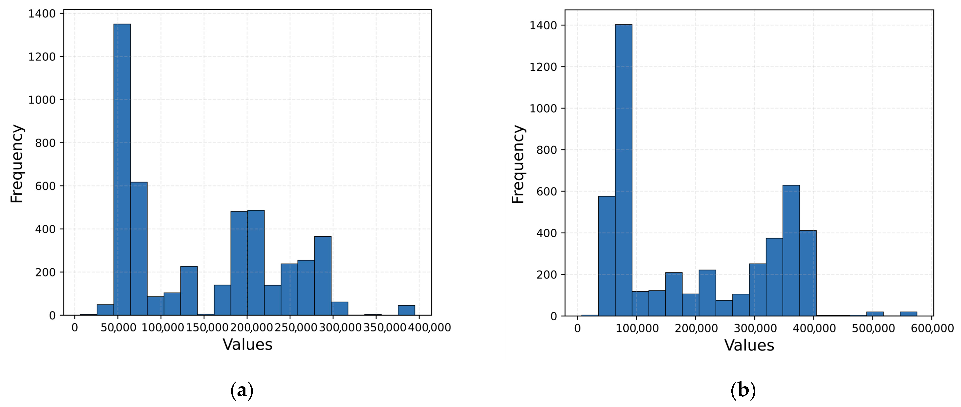
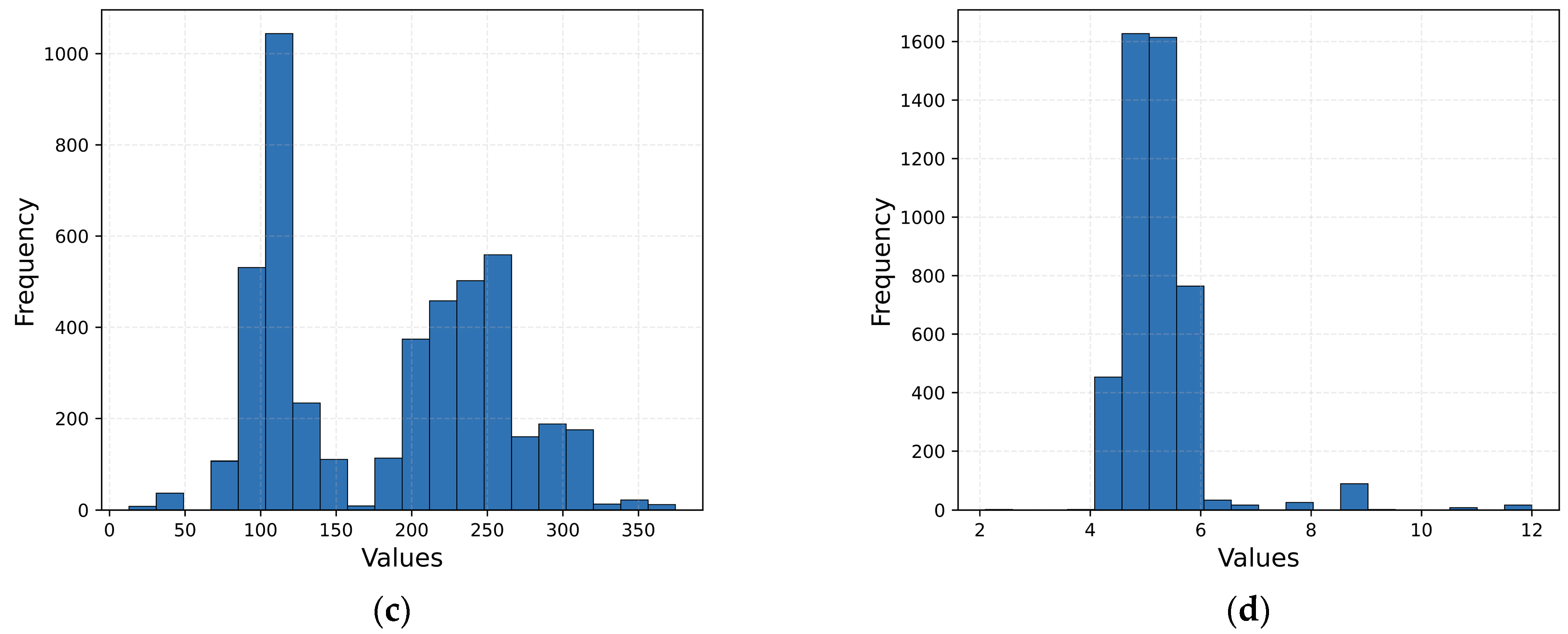
Histogram is an indicator of the frequency distribution, which is the rate of repetition of data within a dataset. Histograms drawn in the form of bar graphs provide an idea about the distribution of the data. The width of the columns depicts the range variation in the data, and the height of the columns indicates the number of observations belonging to each data class, that is, the frequency.

Figure 3 illustrates the histograms for the input features. Examining the histogram of the MLM feature in Figure 2 reveals that the graph is divided into 10 classes. It can be observed that the frequency of data within the range of 0–50,000 is nearly zero, whereas the frequency of data within the range of 50,000 to approximately 80,000 is around 2000. Additionally, the graph, when assessed holistically, demonstrates a distribution deviating slightly from normality. Other input features, such as MTOM, T/O Thrust/Power, and B/P Ratio, can also be analyzed.

The minimum, maximum, mean, median, skewness, and kurtosis values of the input features are presented in

Table 2. Statistical data of the input features.

Features	Min	Max	Mean	Median	Skewness	Kurtosis
MLM (kg)	6450	395,000	149,253.33	135,000	0.404	−1.13
MTOM (kg)	7158	575,000	200,295.35	159,211	0.331	−1.43
TO Thrust/Power (kN/kW)	12.9	374.5	183.68	208.88	0.05	−1.26
B/P Ratio	2.1	12	5.23	5.10	3.49	18.58

. Skewness and kurtosis values are statistical expressions used to characterize the shape of the distribution. Skewness is an indicator of how far the distribution deviates from a symmetric shape with respect to the x-axis. If skewness is between (−0.5)–(+0.5), the distribution is approximately symmetric. In addition, a positive skewness indicates that the distribution is skewed to the right, and a negative skewness indicates that the distribution is skewed to the left. Skewness increases as it moves further away from the (−0.5)–(+0.5) range. Kurtosis is a measure of the sharpness of the distribution with respect to the y-axis. If kurtosis is equal to 0, the distribution is called mesokurtic. The distribution is considered symmetric and balanced. If kurtosis is greater than 0, i.e., positive, it is called leptokurtic. It means that the distribution has a sharp peak and heavy tails. If kurtosis is less than 0, in other words, if it is negative, it is called platykurtic. The distribution is flat, basic, and has light tails.

When the statistical values of the B/P ratio input feature are examined in Table 2, it is seen that the minimum, maximum, mean, median, skewness, and kurtosis values are 2.1, 12, 5.23, 5.10, 3.49, and 18.58, respectively. Since the skewness value of the B/P ratio is 3.49, it can be said that it is skewed to the right, and since the kurtosis value is 18.58, it has a sharp peak. In addition, it is observed that the B/P ratio input feature data is far from a normal distribution. When the skewness and kurtosis values of the other input features are examined, they exhibit a distribution close to normal.

In order to approximate data that does not show a normal distribution, such as the B/P ratio, to a normal distribution, various transformation operations such as logarithm, square root, reciprocal transformation, and Box–Cox are applied to the data mathematically. Thus, the data is transformed into a state closer to a normal distribution. Although transforming data may not have a significant effect on the prediction performance of deep learning models, it is extremely important when making predictions using traditional machine learning methods.

Since the B/P ratio input data does not follow a normal distribution, data transformation was applied. Logarithmic and Box–Cox transformations were preferred for this purpose. Logarithmic transformation involves taking the natural logarithm of each data in the dataset. In order to apply a logarithmic transformation, the data must be greater than zero and positively skewed. Since the values in the B/P ratio feature are greater than zero and the skewness is 3.49, indicating a right-skewed distribution, the logarithmic transformation was applied to this dataset. The natural logarithm function is shown in Equation (5).

$$y={log}_e\left(x\right)$$

(5)

The Box–Cox transformation is one of the methods applied to approximate data to a normal distribution. Similarly to the logarithmic transformation, the data must be positive in order to apply the Box–Cox transformation. The mathematical expression of the Box–Cox transformation is given in Equation (6), where λ (lambda) represents the transformation parameter [30].

$$y={\displaystyle \frac{{(x}^{\lambda }-1)}{\lambda }}$$

(6)

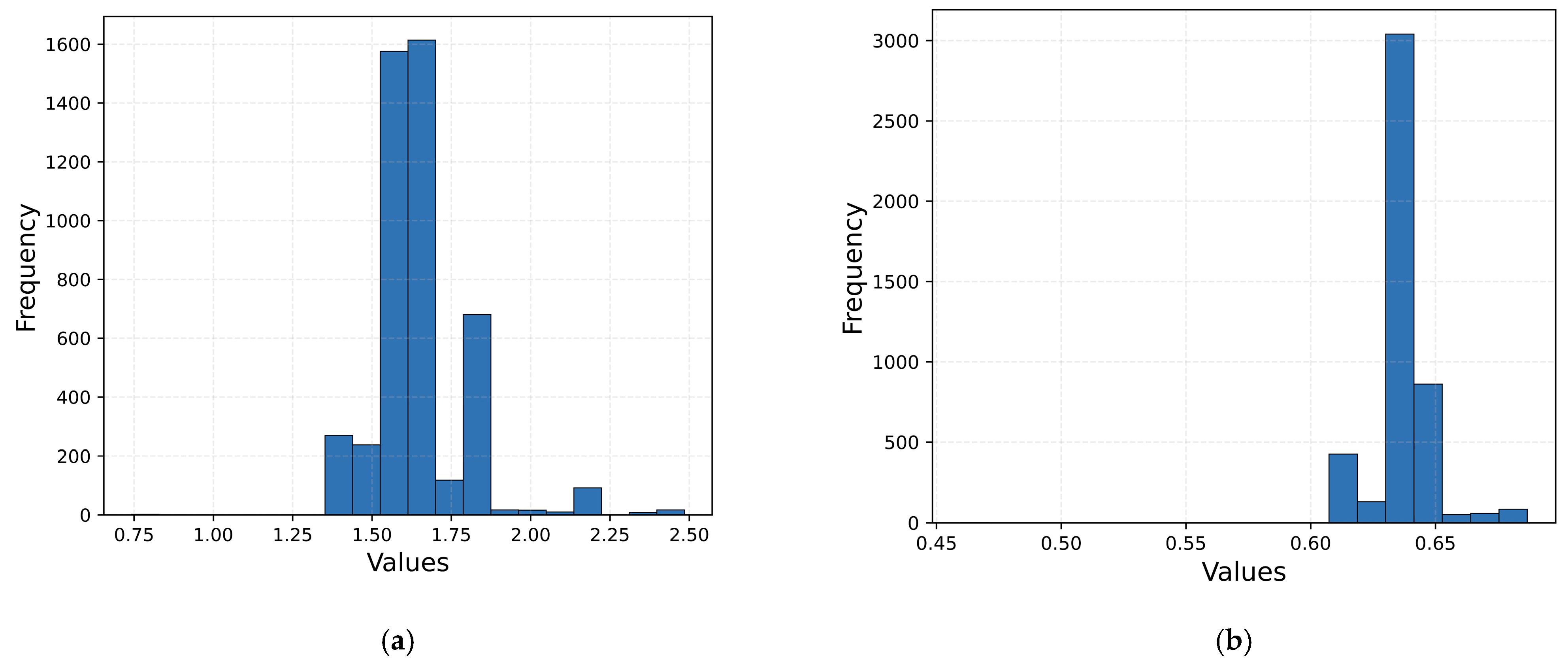
The histogram graphs of the logarithmic and Box–Cox transformations of the B/P ratio input data are shown in Figure 4. When the histogram of the raw B/P ratio data in Figure 3 is compared with the transformed histograms in Figure 4, it can be observed that the data transformed using the logarithmic method is graphically closer to a normal distribution.

The statistical values of the raw B/P ratio input data were compared in detail considering Table 2, which contains the statistical metrics, and

Table 3. Skewness and kurtosis of the B/P ratio data subjected to logarithm and Box–Cox transformation.

Transformation	Skewness	Kurtosis
Logarithm	1.95	8.75
Box–Cox	−0.63	18.46

, which includes the transformation processes. The initial skewness value of the raw data was 3.49, and the kurtosis value was 18.58, both notably high. The high skewness and kurtosis values mean that the distribution is seriously skewed to the right and influenced by extreme values.

After the applied logarithmic transformation, the skewness reduced to 1.95 and the kurtosis to 8.75, making the distribution more symmetrical and closer to a normal distribution. Additionally, the impact of extreme values was considerably reduced. With the Box–Cox transformation, the skewness was obtained as −0.63 and the kurtosis as 18.46. Although the Box–Cox transformation was successful in terms of symmetry by further reducing the skewness, it was not effective in reducing the kurtosis value.

Therefore, the logarithm transformation was preferred because it provided a significant improvement in reducing the skewness and significantly reduced the effect of extreme values. In addition, logarithm transformation offers the advantage of being an easy and highly interpretable method that can be applied to positive continuous data.

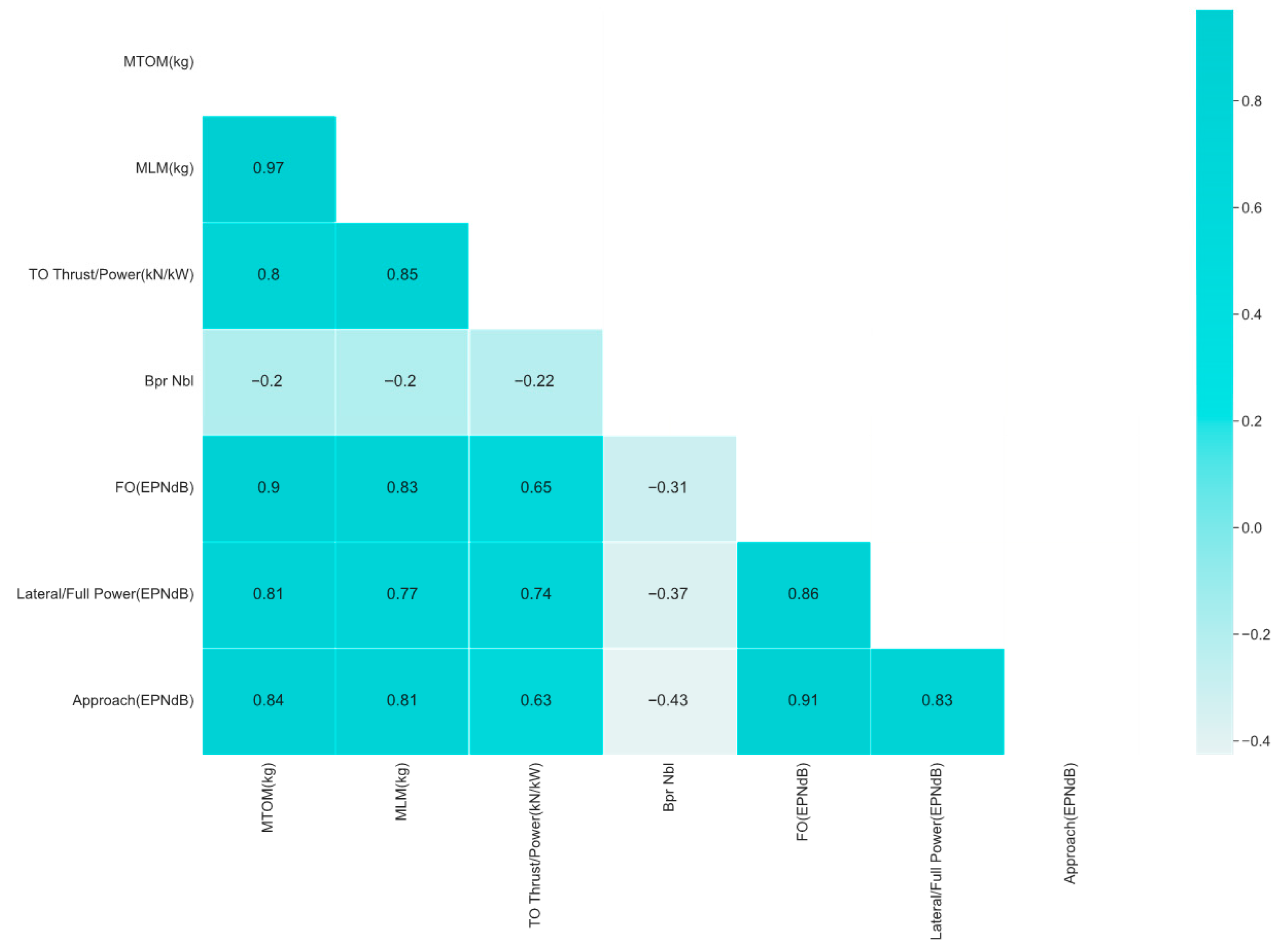
As shown in Figure 5, strong positive correlations are observed between aircraft mass, thrust/power, and noise levels across the three certification points (flyover, lateral, and approach), whereas the bypass ratio exhibits negative correlations. These correlation patterns confirm the nonlinear nature of the data, indicating that linear models would be insufficient to capture the complex relationships among variables. Therefore, nonlinear regression (SVR) and hybrid deep learning (CNN–Transformer) approaches were selected to model both localized and global dependencies.

3.3. Support Vector Regression (SVR)

Support vector regression is a classification algorithm used to determine the best hyperplane to separate data into two or more classes. Smola and Scholkopf [31] developed the SVR model to overcome the regression difficulties [31]. A nonlinear mapping method is used in this approach to map the data into a high-dimensional feature space. This feature distinguishes it from other regression-based models and allows for accurate predictions. In addition, the kernel functions allow linear separation, allowing the data to be transferred to a high-dimensional feature space [32]. During the training of the model, the SVR model is fitted to the training data. This involves solving a convex optimization problem to find the hyperplane that best fits the data. To prevent model overfitting and to tune the model hyper-parameters, cross-validation is used. The evaluation of the model is performed using metrics such as R-squared, MSE, RMSE, MAE, or MAPE. The generalization ability of the model is evaluated on the validation set. Finally, model deployment involves saving the trained SVR model for future use and deploying the model to a real-world application to make continuous predictions. Equation (7) defines the traditional regression function as follows:

$$f\left(x\right)=(w.\mathsf{\Phi }\left(\mathrm{x}\right)+b)$$

(7)

where Φ is denoted the nonlinear mapping of the input to a higher-dimensional feature space, while bias is represented by b.

Equations (8)–(11) express the restricted optimization problem whereas slack variables ${\mathsf{\xi }}_i$ and ${\mathsf{\xi }}_i^{\ast }$ denote the permissible deviations from the insensitive loss function. Moreover, W, ε and C represent weight vector, an insensitive loss function and a penalty factor, respectively, in order to reduce training errors [33,34].

$$\mathsf{\Phi }\left(\mathrm{w},\mathsf{\xi }\right)={\displaystyle \frac{1}{2}}{\left|\right|w\left|\right|}^2+C\sum _{i=1}^N({\mathsf{\xi }}_i+{\mathsf{\xi }}_i^{\ast })$$

(8)

$$\left(\left(w{x}_i\right)+b\right)-y_i\le {\mathsf{\xi }}_i+\varepsilon$$

(9)

$$y_i-\left(\left(w{x}_i\right)+b\right)\le {\mathsf{\xi }}_i^{\ast }+\varepsilon$$

(10)

$${\mathsf{\xi }}_i^{\ast }\ge 0, {\mathsf{\xi }}_i\ge 0 for i=1,2,3, \dots ., n$$

(11)

Equation (12) provides the radial basis function equation as follows:

$$K\left(x_i,x\right)=exp\left[-{\displaystyle \frac{{\left|\right|x-x_i\left|\right|}^2}{2{\sigma }^2}}\right]$$

(12)

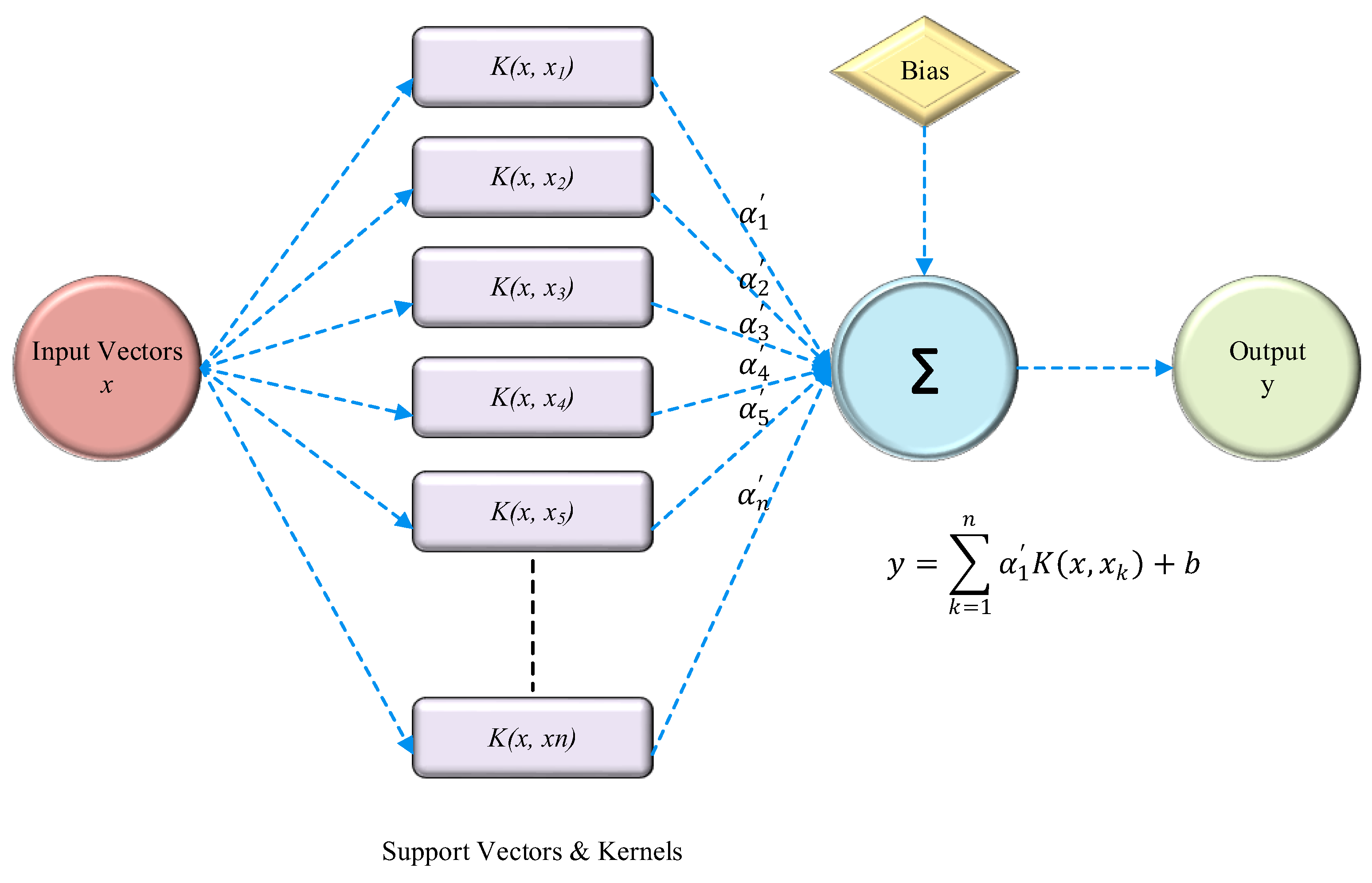
As kernel functions, radial basis function, polynomial, and linear are investigated in this work. Equation (13) may be used to define the decision function once the kernel function has been introduced.

$$f\left(x\right)=\sum _i^n\left({\alpha }_i-{\alpha }_i^{\ast }\right)·K\left(x,x_i\right)+b$$

(13)

Lastly, Figure 6 shows the basic architecture of the SVR method [35].

3.4. Multi-Layer Perceptron (MLP)

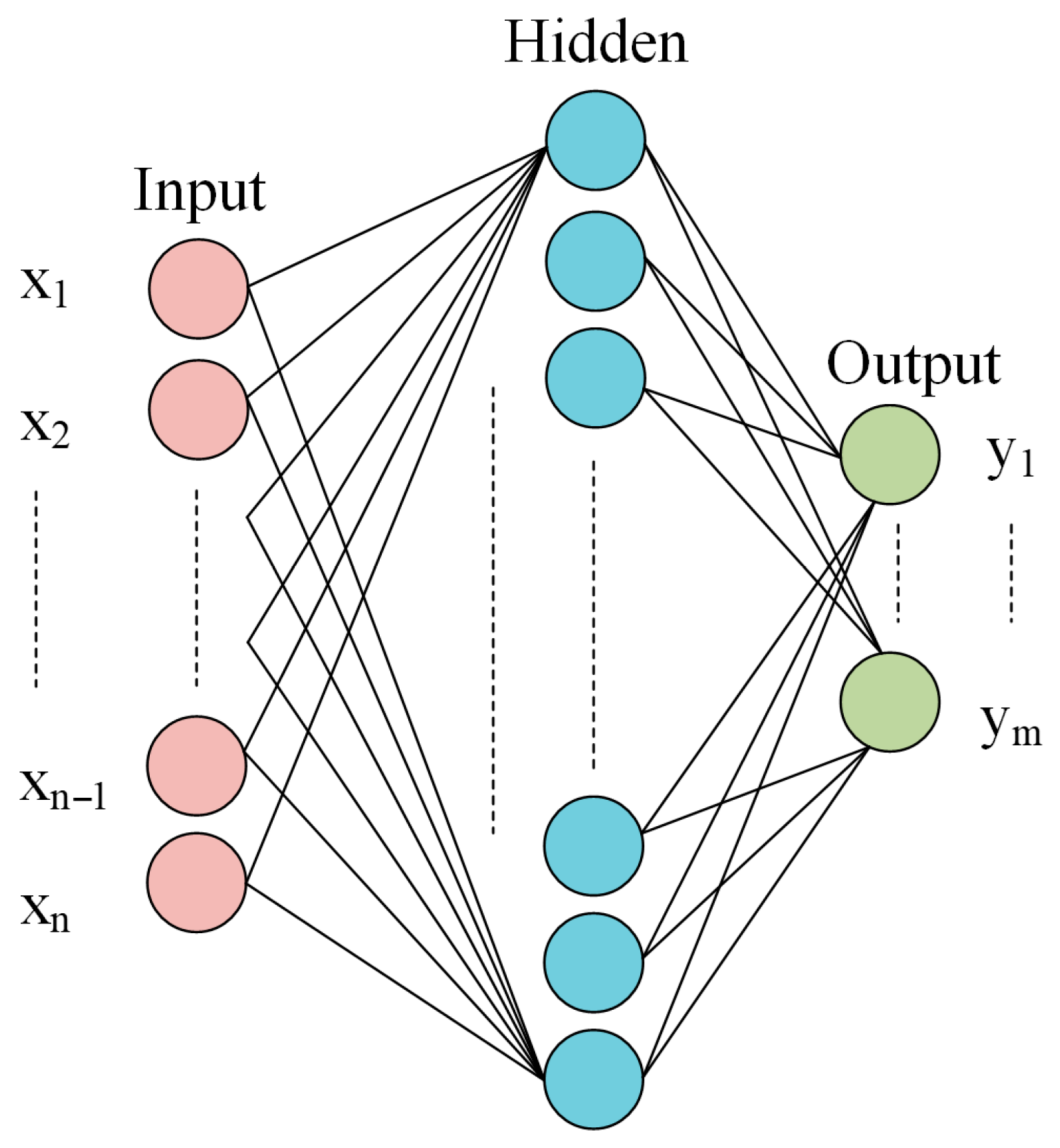
A multi-layer perceptron is a widely used neural network consisting of an input layer, hidden layers, and an output layer, each containing a series of perceptual elements known as neurons. In neural network interactions, each node connected to neurons has a specific bias.

The input layer consists of n input variables $X=\{x_1, x_2, \dots , x_n\}$ while the output layer consists of m output variables $Y=\{y_1, y_2, \dots , y_m\}$. The total number of parameters in a multi-layer perceptron (MLP) can be calculated using Equation (14).

$$n·h_1+\sum _{k=1}^{N_h-1}{h}_k·h_{k+1}+h_{N_h·}n$$

(14)

where the number of hidden nodes $h_i$ in the ith layer is $N_h$. If $N_h$ and $h_k$ are higher, longer computational times are required for optimization of MLP [36]. The fundamental structure of the MLP is given in Figure 7.

3.5. Convolutional Neural Network (CNN)

Convolutional Neural Networks (CNNs), a type of feed-forward deep learning architecture, are primarily composed of convolutional computations. Traditionally utilized in image processing applications, CNNs have recently gained prominence in pattern recognition and classification tasks. Among its layers, the convolutional layer is the most frequently employed. Data is processed through various filters before being forwarded to subsequent layers. The filtered information transferred from the convolution layer to the next layer is called feature maps. The classification performance of this filtered and feature-mapped data is significantly enhanced through convolution operations. In datasets consisting of sequential data, a one-dimensional convolutional structure is applied. Within each convolutional layer, computations are performed using nonlinear activation functions. Among the most commonly utilized activation functions are sigmoid, tanh, and ReLU [37]. The mathematical basic structure of the CNN model is given in Equation (15) where the input value of layer (l − 1) is denoted as ($x_i^{l-1}$), while the convolution kernel is represented as ($w_{ij}^{l-1}$). The threshold value of layer (l) is indicated as ($a_j^l$). F_l−1 denotes the set of input features, and conv1D refers to one-dimensional convolution. y represents the complete feature map, whereas $y_j^l$ corresponds to the feature map within layer (l) [37].

$$y_j^l=ReLU\left(\sum _{i=1}^{F_{l-1}}conv1D(x_i^{l-1}, w_{ij}^{l-1})+a_j^l\right)$$

(15)

3.6. Transformer

The Transformer is a novel neural network architecture based solely on attention mechanisms and operates independently of traditional RNN or CNN architectures designed for sequential data, as proposed by Vaswani et al. [38]. This model is particularly suited for tasks requiring sequential input–output relationships, especially in machine translation. The basic purpose of utilizing the transformer is to enhance the ability to model long-term dependencies while eliminating the need for sequential computation, thereby making the training process more parallelizable and efficient. The model establishes direct connections between all positions in the input via the self-attention mechanism, enabling each position to interact with all other positions.

The key advantages of this approach include more effective learning of long-term dependencies through shorter information transfer paths, significant speed improvements due to parallel computation, reduced training time, and lower computational cost. Furthermore, the model’s interpretability improves, and multi-faceted representation learning is achieved through the use of multiple attention heads.

The transformer model proposed by Vaswani et al. [38] consist of an encoder–decoder architecture, with both components comprising multi-head self-attention mechanisms and fully connected layers. The encoder consists of six identically structured layers, each composed of two fundamental sub-layers. The first is a multi-head self-attention mechanism, and the second is a position-wise feed-forward network. Residual connection is added to each of these sub-layers. Then, layer normalization is applied.

Leveraging the multi-head feature, this process is executed in parallel across different content spaces, allowing each head to capture distinct types of dependencies. The mathematical expression for the scaled dot-product attention mechanism is presented in Equation (16). The multi-head attention mechanism operates as the parallel execution of several scaled dot-product attention mechanisms, with their outputs subsequently summed. The structure of the multi-head attention mechanism is described in Equation (17) where Q, K, V, d_k and W^O, respectively, denote queries, keys, values, the size or dimensionality of the input, and the weight matrix of the output.

$$Attention \left(Q, K, V\right)=softmax({\displaystyle \frac{Q{K}^T}{\sqrt{d_k}}})V$$

(16)

$$\begin{array}{c} MultiHead \left(Q,K,V\right)=Concat ({head}_1, \dots , {head}_3)W^O\\ \mathrm{where} {head}_i=Attention (Q{W}_i^Q, K{W}_i^K, V{W}_i^V)\hfill \end{array}$$

(17)

A position-wise feed-forward network (FFN) is a small neural network consisting of two linear transformations with a ReLU activation function applied between them. These transformations are independently applied to each position. The FFN is defined in Equation (18) where x represents the input vector, corresponding to the output obtained after the attention process for a given position within the encoder or decoder layer. W denotes the weight matrix of the linear transformation, while b represents the bias vector associated with the transformation.

$$FFN \left(x\right)=\max \left(0, x{W}_1+b_1\right)W_2+b_2$$

(18)

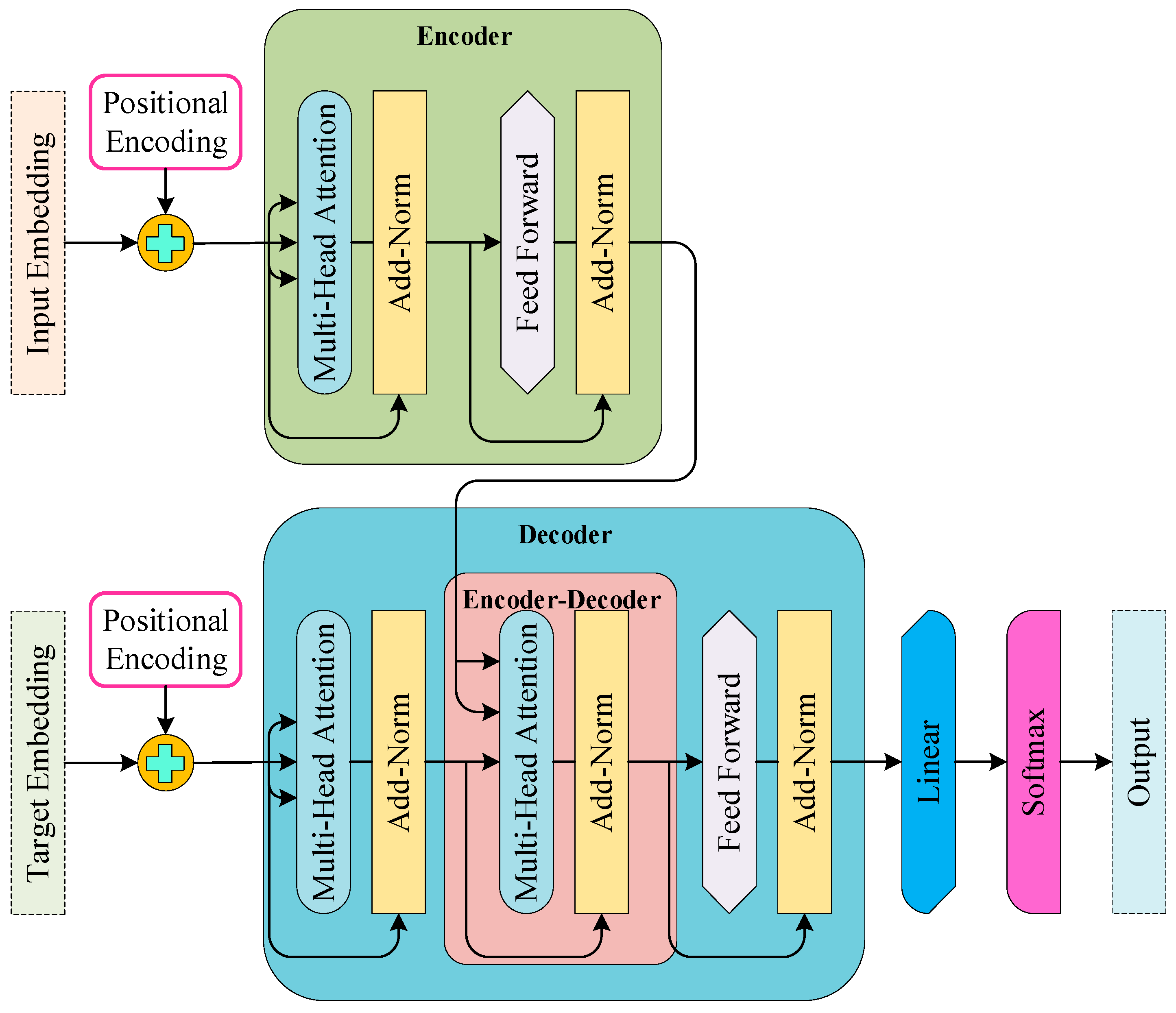
The decoder incorporates a third sub-layer in addition to the standard encoder structure. This additional sub-layer, known as the encoder–decoder attention layer, applies attention to the encoder’s output. Furthermore, within the decoder’s self-attention mechanism, a masking process is implemented to restrict access to future positions. This approach ensures that predictions are made solely based on prior observations. To incorporate positional information, the model utilizes positional encoding, which can either be learned or derived from fixed sine and cosine functions, enriching both encoder and decoder inputs. The transformer’s architecture is shown in Figure 8. Finally, the transformer operates entirely on attention mechanisms, removing sequential dependencies and facilitating efficient, highly parallelized representation learning with lower computational cost [38].

3.7. Proposed CNN–Transformer Hybrid Model

A deep learning model was employed to process data obtained from the aircraft noise modeling database, which includes features such as MLM, MTOM, take-off thrust, and B/P ratio. The model estimated noise measurement output for approach, lateral, and flyover points. CNN–Transformer hybrid model was used as a deep learning model.

Although the number of input variables is limited to four (MLM, MTOM, take-off thrust/power, and bypass ratio), these parameters exhibit nonlinear couplings (e.g., mass–thrust and thrust–bypass effects) that vary across certification points. To represent these relationships effectively, a shallow 1-D convolution is employed across the feature axis to capture localized inter-feature interactions with shared weights, introducing a regularizing inductive bias and avoiding over-parameterization. The Transformer encoder then models global cross-feature dependencies through multi-head self-attention, enhancing nonlinear mapping capability and generalization across aircraft types and flight phases. SVR is retained as a strong classical baseline, and an MLP baseline is included for completeness. All models use identical preprocessing and data splits, and hyper-parameters are tuned via grid search; comparative results as seen in results table show that the hybrid CNN–Transformer consistently attains lower MSE/RMSE/MAE and higher R² than the baselines.

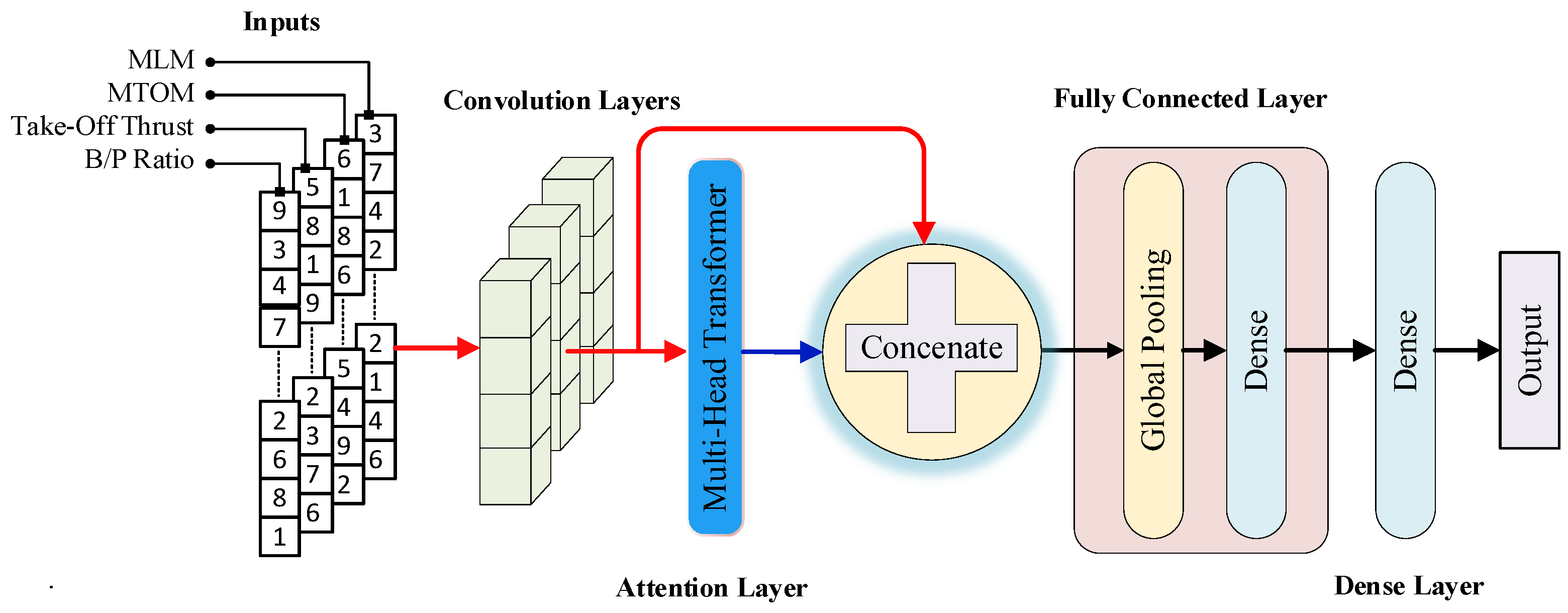
A hybrid model architecture designed to process multivariate time series data, integrating both convolutional (CNN) and attention-based (multi-head attention) mechanisms is shown in Figure 9. Firstly, the input data is passed through one-dimensional convolutional layers to extract local features. The extracted features are sent both directly and to the multi-head attention module to model long-term dependencies. The outputs of the CNN and attention layers are combined to form a unified representations, and this representation is transferred to a Fully Connected Layer consisting of Global Average Pooling and fully connected (Dense) layers. These layers reduce the feature dimension and produce the prediction output for the regression target, respectively.

In the Google Colab environment, the Keras library is used to obtain SVR and CNN–Transformer models. Ablation was performed to analyze the effect of parameters and hyper-parameters on the model and to find the parameter and hyper-parameter combination with the highest performance. The most popular technique for parameter and hyper-parameter optimization is grid search. In grid search, all possible parameters and hyper-parameters are tested, and those that yield the best results are used. In this context, grid search was utilized in this work to find the SVR parameters and CNN–Transformer hyper-parameters. Four different feature data are provided as the inputs. With the Grid Search algorithm, the C parameter was tested in the range of 0.5–1 and the epsilon parameter was tested in the range of 0.001–0.005 for the SVR model. As the kernel function, the functions “linear”, “poly”, “rbf” and “sigmoid” were tested. For the MLP model, the hyper-parameters were optimized using the Grid Search algorithm. The following parameter ranges were tested: “Batch size = 2, 4, 8”, number of neurons per “hidden layer = 16, 32, 64”, and “learning rate (lr) = 0.001, 0.0001”. For the CNN–Transformer model, the hyper-parameters were tested with the Grid Search algorithm with the combinations of the values “Batch Size = 2, 4, 8” and “learning rate (lr) = 0.001–0.0001”. For the CNN layer, the hyper-parameter value combinations “filters = 8, 16, 32”, “kernel_size = 5, 7, 9”, “activation = relu, tanh” and for the multi-head attention layer, the hyper-parameter values “num_heads = 2, 4, 8”, “ff_dim = 32, 64, 128” and “hid_dim = 32, 64, 128” were tested with the Grid Search algorithm. The outputs are predicted using the single-output dense layer.

Table 4. Grid search results for SVR parameters.

SVR	C	Cache Size	ε	Gamma	Kernel Function
	1	200	0.001	Scale	rbf

provides the SVR parameters,

Table 5. Grid search results for MLP.

MLP	Activation Function	Loss Function	Optimizer	Batch Size	lr	Neuron
	ReLU	MSE	Adam	4	0.0001	64

gives the MLP hyper-parameters, and

Table 6. Grid search results for CNN–Transformer hyper-parameters.

CNN–Transformer	Activation Function	Loss Function	Optimizer	Batch Size	lr	Filters Kernel Size	Num_Head Ff_Dim Hid_Dim
	ReLU	MSE	Adam	2	0.0001	32 5	8 128 128

shows CNN–Transformer model’s hyper-parameters. Upon applying grid search to both models, the SVR model yields “C = 1”, “ε = 0.001”, “gamma = scale”, and “kernel function = rbf”.

The dataset comprised 4656 total samples, divided into 90% for training (4190) and 10% for testing (466). Early stopping was applied to prevent overfitting. The CNN–Transformer model converged after 50 epochs, while the MLP stopped at 25 epochs. Hyper-parameters were optimized using grid search, with the best results achieved using a batch size of 2 for the CNN–Transformer and 4 for the MLP model. The optimal learning rate was 0.0001 for both architectures, and the Adam optimizer with MSE loss function provided the best performance.

For the MLP model, the ReLU activation function, mean squared error (MSE) loss function, and Adam optimizer provided the best convergence performance. The optimal configuration, “Batch size = 4”, “lr = 0.0001”, and “64 neurons”, was selected for the final model. The summary of the grid search results is presented in Table 5.

On the other hand, the hyper-parameters of the CNN–Transformer model are obtained as “batch size = 2”, “learning rate (lr) = 0.0001”, “optimizer = Adam”, “activation function = relu” and “loss function = MSE”, “filters = 32”, “kernel_size = 5”, “num_heads = 8”, “ff_dim = 128” and “hid_dim = 128” and are given in Table 6. During training, MSE between the predicted and actual EPNL values was used as the loss function to evaluate model convergence.

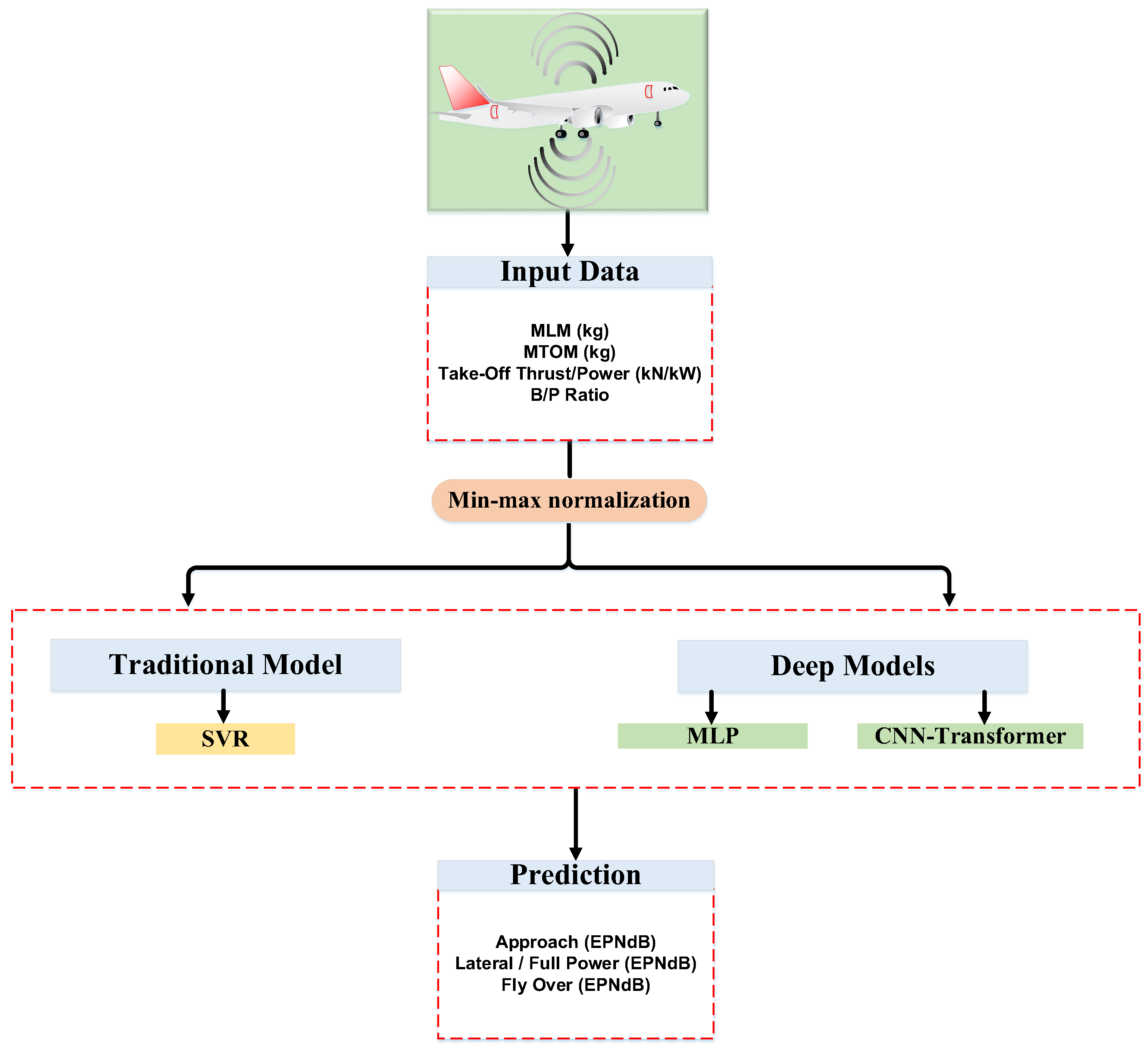
Figure 10 presents a flowchart detailing the step-by-step process for estimating aircraft noise, ensuring clear comprehension. The required data is first extracted from the database and then processed separately using both traditional and deep learning models. Subsequently, predictions related to aircraft noise are generated and evaluated using several error metrics, which indicate the extent to which the models effectively predict the determined outputs.

3.8. Evaluation Metrics

To evaluate the modeling success of both approaches, four error metrics, MSE, root mean square error (RMSE), mean absolute error (MAE), and mean absolute percentage error (MAPE), are employed to quantify the differences between actual and predicted values. Additionally, the coefficient of determination (R²) is calculated for each efficiency model, aiming for a value as close to unity as possible [33,37]. In Equations (19)–(23), y represents the actual values, $\overline{y}$ denotes the estimated values, and $\widehat{y}$ corresponds to the arithmetic mean of the actual values, respectively [7,39].

$$MSE={\displaystyle \frac{1}{n}}\sum _{i=1}^n{\left({y_i-\overline{y}}_i\right)}^2$$

(19)

$$RMSE=\sqrt{{\displaystyle \frac{1}{n}}\sum _{i=1}^n{\left({y_i-\overline{y}}_i\right)}^2}$$

(20)

$$MAE={\displaystyle \frac{1}{n}}\sum _{i=1}^n\left|{y_i-\overline{y}}_i\right|$$

(21)

$$MAPE={\displaystyle \frac{1}{n}}\sum _{i=1}^n\left|{\displaystyle \frac{{y_i-\overline{y}}_i}{y_i}}\right|$$

(22)

$$R^2=1-{\displaystyle \frac{\sum _{i=1}^n{\left(y_i-{\overline{y}}_i\right)}^2}{\sum _{i=1}^n{\left(y_i-\widehat{y}\right)}^2}}$$

(23)

4. Results and Discussion

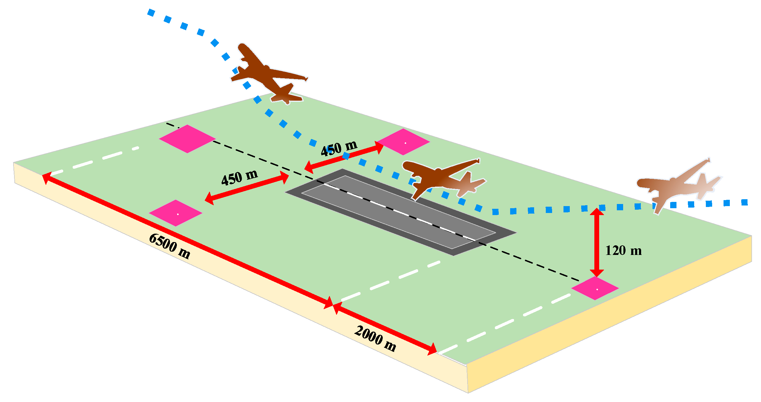
In this study, the noise levels generated by Airbus and Boeing aircraft were predicted at ICAO reference points by applying two different modeling approaches: Support vector regression (SVR) and a hybrid deep learning architecture combining CNN and Transformer layers. Predictions were performed at the three primary measurement locations defined in ICAO Annex 16 regulations: approach, lateral/full power, and flyover.

Noise levels recorded at ICAO measurement points are determined by well-defined aeroacoustic mechanisms in aviation acoustics theory. At the approach point, the dominant noise sources are fan broadband noise that emerges at low engine thrust and airframe noise originating from high-lift surfaces such as flaps and landing gear [10,26]. At the lateral measurement point, engine–ground interaction, jet mixing noise, and turbulence structures come to the fore, and due to reflection and diffraction effects, the noise field exhibits more complex acoustic behavior [25,28]. At the flyover point, since the engine operates at maximum thrust, high-level turbulent jet noise becomes dominant with the increase in jet velocity [21,28]. These physical differences cause the noise characteristics at the three measurement points to be distinctly separated from each other.

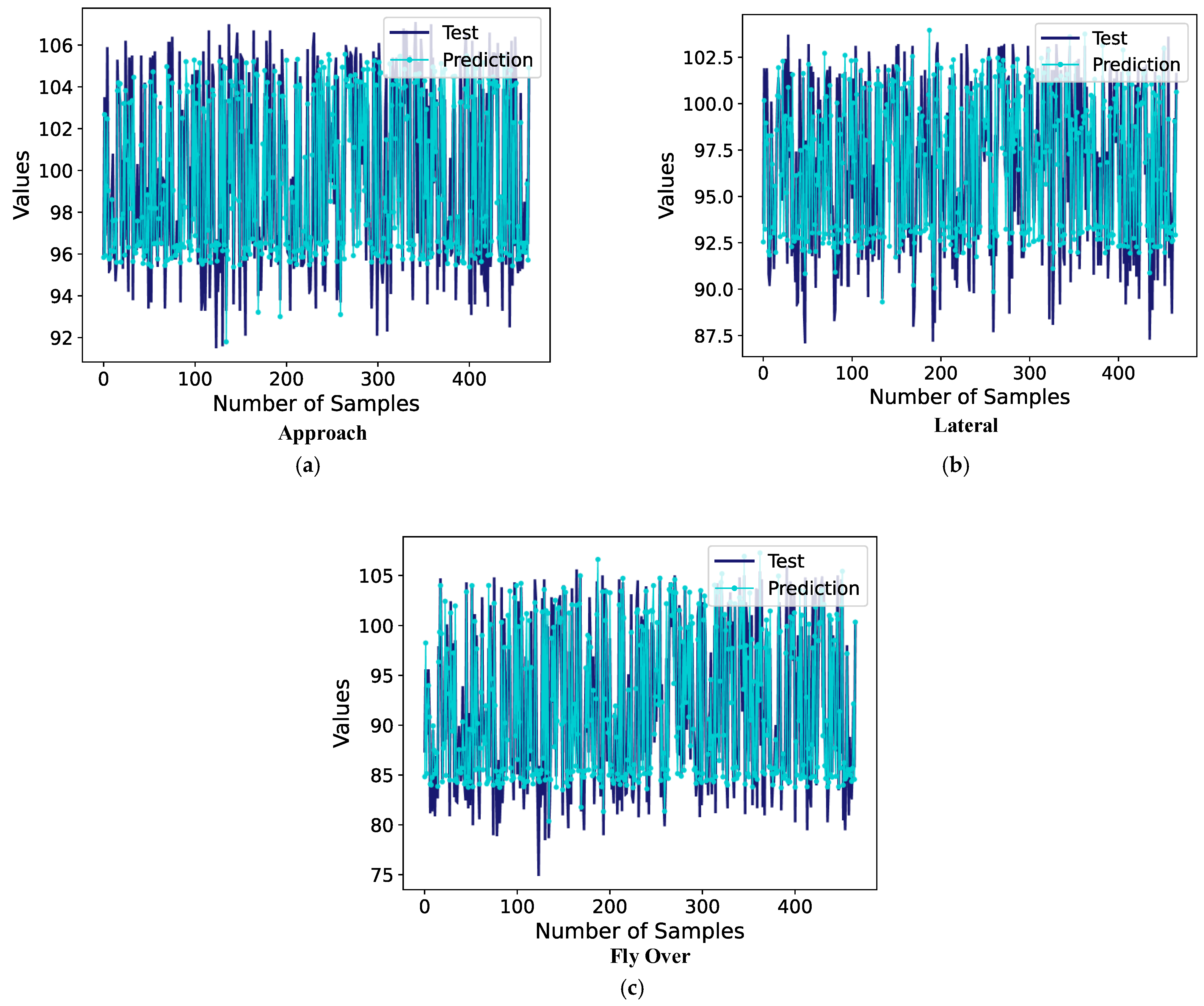
In this section, the prediction performance of both models is detailed with figures and tables, and comparative analyses are presented. Figure 11 shows that the SVR model’s predictions compare with the actual test data. Overall, the predictions are close to the observed values. At certain points, notable discrepancies are observed between the predicted values and the actual test data.

An examination of

Table 7. Test and predicted values of noise for approach, lateral, and flyover.

Model	Approach (EPNdB)		Lateral/Full Power (EPNdB)		Flyover (EPNdB)
SVR	Test	Prediction	Test	Prediction	Test	Prediction
	96	95.843	93.6	92.549	87.4	84.843
	103.4	102.68	101.8	100.17	95.4	98.273
	97	95.929	98.2	93.242	89.1	85.162
	98.7	99.259	99.1	98.965	89.2	91.904
	105.8	102.47	101.6	97.849	95.4	93.999
	98.9	99.041	97.8	98.276	91.6	90.840
	95.2	95.768	90.8	92.040	81.4	84.102
	95.3	95.828	90.3	91.846	82.6	84.016
	98.5	96.173	91.2	92.800	81.6	84.773
	98.9	98.610	100	98.282	89.3	89.943
	100.7	97.596	96.7	96.740	85.6	87.507
	95.9	96.130	94.7	93.350	81.1	85.132
	96.6	96.504	91.2	93.041	86.7	85.547
	94.8	97.633	94.2	95.565	84.2	87.236
	95.5	95.610	92.2	91.988	82.9	83.873
MLP	Test	Prediction	Test	Prediction	Test	Prediction
	96	95.126	93.6	92.321	87.4	84.640
	103.4	102.57	101.8	99.108	95.4	97.175
	97	95.534	98.2	95.821	89.1	85.941
	98.7	99.079	99.1	97.998	89.2	90.911
	105.8	103.07	101.6	98.143	95.4	94.792
	98.9	99.137	97.8	97.485	91.6	90.436
	95.2	95.318	90.8	90.104	81.4	82.301
	95.3	95.515	90.3	89.417	82.6	82.890
	98.5	96.101	91.2	91.782	81.6	82.520
	98.9	98.812	100	97.405	89.3	89.075
	100.7	98.344	96.7	96.375	85.6	87.937
	95.9	96.019	94.7	94.278	81.1	82.537
	96.6	96.344	91.2	92.506	86.7	86.241
	94.8	98.377	94.2	94.816	84.2	86.705
	95.5	95.031	92.2	91.491	82.9	83.354
CNN–Transformer	Test	Prediction	Test	Prediction	Test	Prediction
	96	94.589	93.6	92.735	87.4	86.170
	103.4	102.60	101.8	101.82	95.4	95.713
	97	96.864	98.2	96.293	89.1	87.454
	98.7	98.486	99.1	98.350	89.2	91.593
	105.8	104.63	101.6	100.88	95.4	94.688
	98.9	99.164	97.8	98.162	91.6	91.365
	95.2	95.249	90.8	90.233	81.4	81.051
	95.3	95.718	90.3	89.256	82.6	82.108
	98.5	97.564	91.2	91.451	81.6	81.900
	98.9	98.412	100	98.135	89.3	89.299
	100.7	98.974	96.7	96.557	85.6	86.888
	95.9	96.095	94.7	94.793	81.1	81.152
	96.6	96.195	91.2	91.723	86.7	87.451
	94.8	95.816	94.2	93.506	84.2	85.415
	95.5	94.190	92.2	91.801	82.9	83.970

and

Table 8. Analysis results of test data using SVR, MLP, and a hybrid CNN–Transformer model.

Model	Outputs (EPNdB)	MSE	RMSE	MAE	MAPE	R2
SVR	Approach	3.183667	1.784283	1.390288	0.013893	0.817406
	Lateral/Full Power	4.253906	2.062499	1.642044	0.017013	0.758226
	Flyover	6.167471	2.483439	1.966880	0.021620	0.898655
MLP	Approach	2.401845	1.549788	1.185135	0.011887	0.862246
	Lateral/Full Power	2.625102	1.620216	1.171423	0.012008	0.850800
	Flyover	4.875596	2.208075	1.619979	0.017675	0.919883
CNN–Transformer	Approach	0.836422	0.914561	0.640903	0.006467	0.952028
	Lateral/Full Power	0.577697	0.760064	0.586077	0.006031	0.967166
	Flyover	1.157550	1.075895	0.789108	0.008762	0.980979

indicates that the SVR model generated an MSE of 3.18, an RMSE of 1.78, and an MAE of 1.39 at the approach point. These evaluation criteria show that the model offers reasonable predictive performance. However, the R² value of 0.817 also suggest that the model has certain limitations in nonlinear data relationships. Considering the data in Table 7, the test values generally range from 95 to 105 EPNdB, and the SVR model’s predictions closely approximate this interval. For instance, for a test value of 103.4 dB, the SVR model predicted a value of 102.68 EPNdB, a difference of only 0.72 EPNdB.

At the lateral point, the SVR model exhibits relatively weak performance with MSE 4.25, RMSE 2.06, MAE 1.64, and R² 0.758. This is particularly evident in the predicted deviations for test values in the 90–100 dB range. For instance, for a test value of 98.2 EPNdB, the model predicted 93.24 EPNdB, representing a significant difference of approximately 5 EPNdB.

At the flyover point, the SVR model achieved a high R² value of 0.898, indicating strong agreement with the test data. However, in the prediction, the SVR model obtained an MAE of 1.96 and an RMSE of 2.48. This suggests that moderate deviations still remain between predicted and actual values. According to Table 7, for a test value of 91.2 EPNdB, the model predicted 92.80 dB, with an error of 1.6 EPNdB.

Figure 11 presents the comparison between the predicted and actual EPNL values for all 466 test samples, illustrating the overall distribution of model predictions across the three ICAO reference points (approach, lateral, and flyover). This visualization complements the numerical results in Table 7 and Table 8 by revealing the consistency and spread of prediction errors, offering a more intuitive understanding of the model’s generalization capability. The strong linear alignment between the predicted and observed values confirms that the model reliably reproduces the certified noise measurements within the 95–105 EPNdB interval.

An examination of Table 8 indicates that the MLP model provided moderate predictive performance compared with the CNN–Transformer and SVR models. At the approach point, the MLP achieved an MSE of 2.40, RMSE of 1.54, and MAE of 1.18, with an R² value of 0.862. Although these results demonstrate acceptable accuracy, the model’s capacity to capture nonlinear dependencies among parameters such as thrust, mass, and bypass ratio remains limited. As seen in Table 7, for a test value of 103.4 EPNdB, the MLP predicted 102.57 EPNdB, corresponding to an error of 0.83 EPNdB.

At the lateral point, the MLP’s predictive capability decreased further (MSE = 2.62, RMSE = 1.62, MAE = 1.18, R² = 0.850). This result reflects the model’s weaker adaptability to the complex, nonlinear behavior of the lateral noise measurements, especially within the 90–100 EPNdB range. As shown in Table 7, for a test value of 93.6 EPNdB, the model produced 92.73 EPNdB, resulting in a difference of 0.87 EPNdB.

At the flyover point, the MLP attained its highest accuracy, with R² = 0.919, MSE = 4.87, RMSE = 2.20, and MAE = 1.61. This finding suggests that the MLP can effectively capture the general nonlinear trend between aerodynamic–engine parameters and noise emissions, though its performance remains below that of the CNN–Transformer model. As given in Table 7, for a test value of 87.4 EPNdB, the MLP predicted 84.64 EPNdB, with a deviation of 1.76 EPNdB.

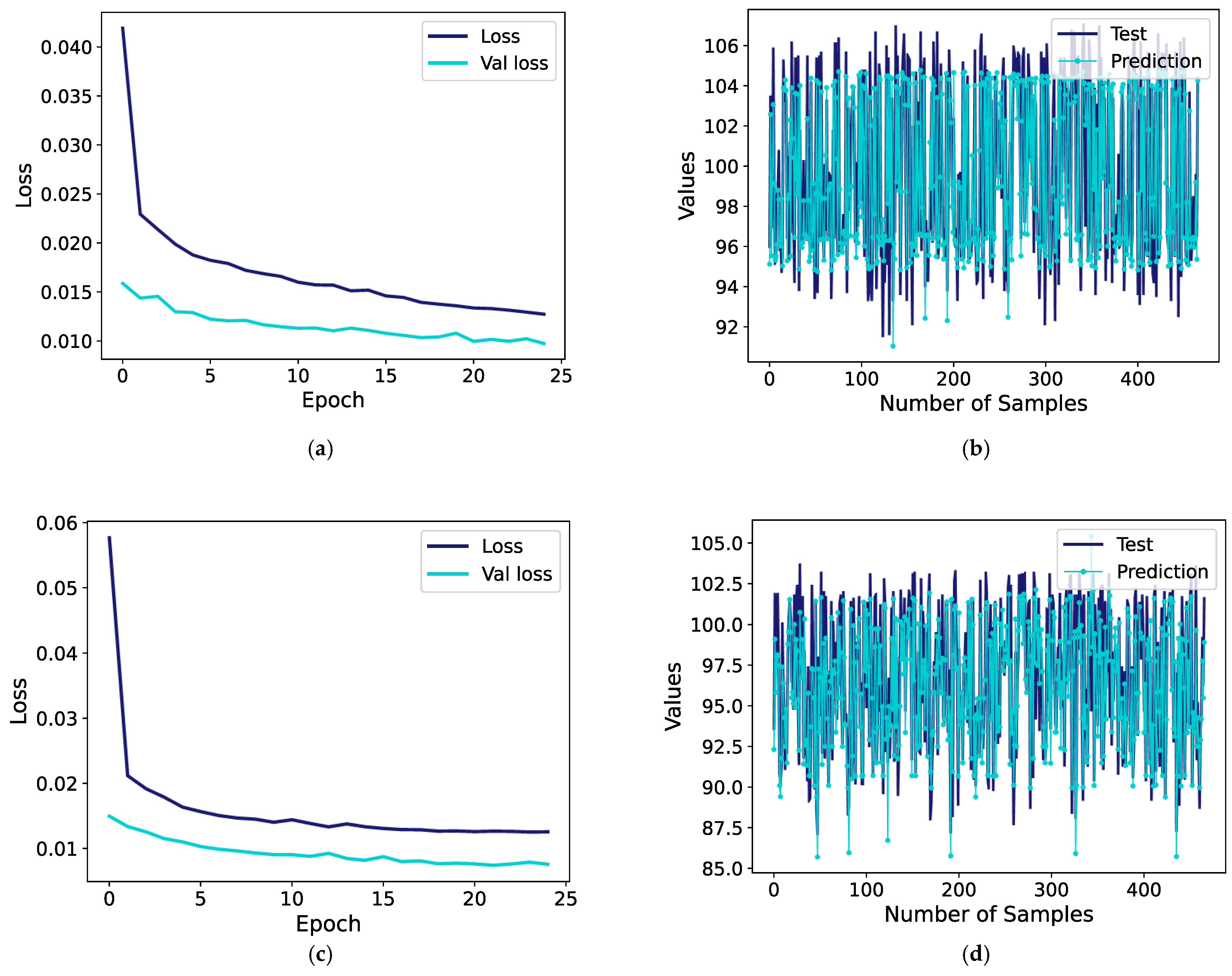
Figure 12 illustrates the training behavior and predictive performance of the MLP model. Figure 12a,c,e show the training and validation loss (MSE) curves for the three reference points, indicating stable convergence and the effect of early stopping, which halted the training after approximately 25 epochs to prevent overfitting. Figure 12b,d,f compare the predicted and actual EPNL values for all 466 test samples, demonstrating that while the MLP captures the general nonlinear trend of the data, residual deviations remain larger than those observed for the CNN–Transformer model. These plots visually support the quantitative results reported in Table 8, confirming that the MLP provides a reasonable baseline but lacks the cross-feature learning capability achieved by the hybrid attention-based architecture.

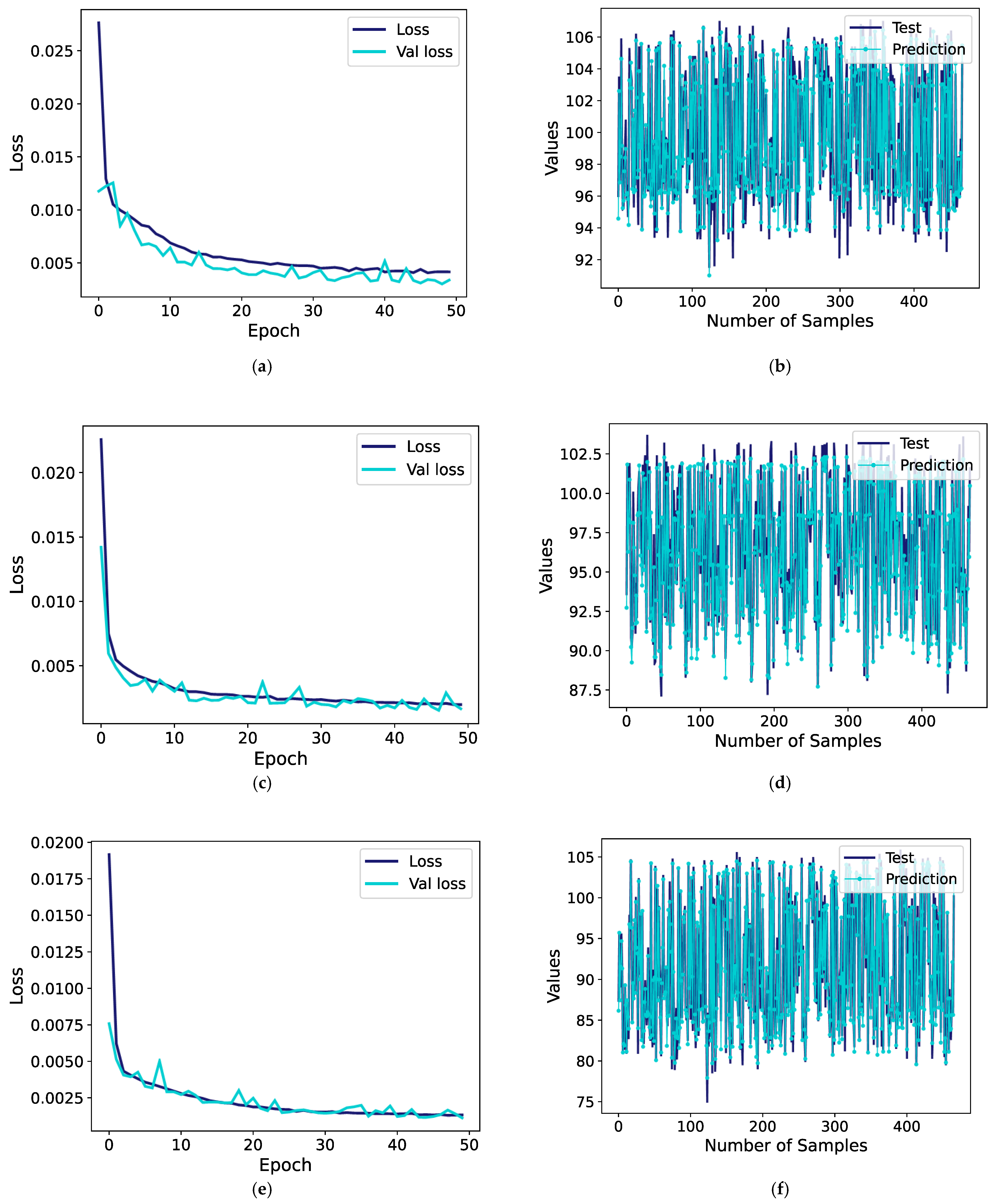
As seen in Figure 13, the prediction values generated by the CNN–Transformer hybrid model exhibit a very high degree of overlap with the test data. The model’s loss function plot indicates that the model maintained stable learning occurred throughout the training process and that overfitting did not occur. The numerical results presented in Table 8 demonstrate that the CNN–Transformer hybrid model significantly outperforms the SVR across all evaluated metrics.

The CNN–Transformer hybrid model predicted an MSE of 0.83, RMSE of 0.91, and MAE of 0.64 at the approach point. Compared to the SVR model, the CNN–Transformer hybrid model predicted with approximately 50% less error at the approach point. The R² value was 0.952, indicating a very high level of accuracy in the model’s predictions. As shown in Table 6, for a test value of 103.4 EPNdB, the CNN–Transformer hybrid model predicted 102.6 EPNdB, resulting in a deviation of just 0.8 EPNdB.

At the lateral point, the CNN–Transformer hybrid model once again outperformed the SVR model, achieving an MAE of 0.58 and an RMSE of 0.76. Also, the R² value reached a very high level of 0.967. The data in Table 6 clearly reinforces the model’s strong performance at this point. For a test value of 94.2 EPNdB, the model predicted a value of 93.5 EPNdB, representing a difference of only 0.7 EPNdB.

At the flyover point, the CNN–Transformer hybrid model achieved an R² value of 0.981, marking the highest level of predictive success observed in this study. The CNN–Transformer hybrid model achieved strong predictive performance, with an MAE of 0.79 and an RMSE of 1.07, reflecting both high precision and accuracy. In the case of a test value of 86.7 EPNdB, the model predicted 87.45 EPNdB, resulting in a minor difference of 0.75 EPNdB.

Figure 13 provides detailed insight into the training dynamics and predictive reliability of the proposed CNN–Transformer model. Figure 13a,c,e depict the training and validation loss curves (MSE), where the early-stopping mechanism halted the training between 25 and 50 epochs, preventing overfitting and confirming stable convergence. Figure 13b,d,f illustrate the predicted versus observed EPNL values for the 466 test samples, showing close agreement between predictions and true values for all reference points. Together, these plots visually demonstrate both the effectiveness of the early-stopping strategy and the robust generalization of the hybrid network.

As seen in Table 8, the CNN–Transformer hybrid model achieved significantly better predictive performance than the MLP and SVR across all metrics. The hybrid model consistently outperformed the baseline, demonstrating superior generalization and reliability under identical preprocessing and data partitioning conditions.

At the approach point, the RMSE value for the SVR and MLP models were 1.78 and 1.54, respectively, while for the CNN–Transformer, it was 0.91. The MAE value for the SVR and MLP models were 1.39 and 1.18, respectively, while for the CNN–Transformer, it was only 0.64. In terms of R² value, CNN–Transformer shows a very high generalization success with 0.952, while this rate is only 0.817 in SVR and 0.862 in MLP.

At the lateral point, the SVR model recorded an RMSE of 2.06 and an MAE of 1.64 and the MLP model recorded an RMSE of 1.62 and an MAE of 1.17, whereas the CNN–Transformer hybrid model achieved markedly lower values of 0.76 and 0.58, respectively. The R² score, which was 0.758 for the SVR, 0.85 for the MLP, and 0.967 for the CNN–Transformer, created a significant difference. This performance gap indicates that the CNN–Transformer hybrid model not only yields fewer prediction errors but also captures broader data trends with greater fidelity.

At the flyover point, the SVR and the MLP models exhibited their highest error rates, with RMSE of 2.48 and 2.20 and MAE of 1.96 and 1.61, respectively, indicating reduced predictive reliability at this reference location. In contrast, the CNN–Transformer hybrid model achieved lower errors, with an RMSE of 1.07 and an MAE of 0.79, indicating improved predictive accuracy. The CNN–Transformer hybrid model also recorded the highest predictive accuracy, with an R² value of 0.981, confirming its strong generalization capacity and robust prediction performance.

In this study, the models were evaluated on the same test dataset. Therefore, MAE and MSE values from MLP, SVR, and CNN–Transformer models for each test sample created correlated observations. In this situation where models produced non-independent, paired error values, a paired t-test was used to test the significance of the mean error difference between two models. Summary statistics for the error performance of the models are given in

Table 9. Paired t-test results comparing MLP, SVR, and a hybrid CNN–Transformer model across three ICAO measurement points (approach, lateral, flyover).

Measurements Point	Model Comparison	Metric	t-Value	p-Value
Approach	MLP vs. SVR	MAE	−14.3400	7.04 × 10−39
		MSE	−11.0476	2.35 × 10−25
	MLP vs. CNN–Transformer	MAE	3.7391	2.08 × 10−4
		MSE	2.7280	6.61 × 10−3
	SVR vs. CNN–Transformer	MAE	14.9319	1.82 × 10−41
		MSE	11.3084	2.32 × 10−26
Lateral	MLP vs. SVR	MAE	−8.3348	8.83 × 10−16
		MSE	−6.0981	2.26 × 10−9
	MLP vs. CNN–Transformer	MAE	11.6098	1.54 × 10−27
		MSE	6.1361	1.81 × 10−9
	SVR vs. CNN– Transformer	MAE	16.1138	9.81 × 10−47
		MSE	12.3916	1.14 × 10−30
Flyover	MLP vs. SVR	MAE	−7.1029	4.61 × 10−12
		MSE	−4.9003	1.32 × 10−6
	MLP vs. CNN–Transformer	MAE	13.0279	2.71 × 10−33
		MSE	5.0605	6.03 × 10−7
	SVR vs. CNN–Transformer	MAE	15.9501	5.35 × 10−46
		MSE	10.3951	6.73 × 10−23

.

The paired t-test results show that the differences between model performances are statistically significant at all three measurement points. At the approach measurement point, the MLP-SVR comparison yielded t-value = −14.3400 and p-value = 7.04 × 10⁻³⁹ according to the MAE metric. The negative t-value indicates that MLP’s mean absolute error value is lower than SVR’s. Similarly, in the MLP, CNN–Transformer and SVR, CNN–Transformer comparisons, the hybrid CNN–Transformer model produced the lowest error values, and all p-values were considerably below 0.01. At the approach point, noise behavior is more variable due to low engine thrust; nevertheless, the hybrid CNN–Transformer model successfully captured complex patterns.

The paired t-test results for the lateral measurement point show a similar trend. For the MLP-SVR comparison, t-value = −8.3348 and p-value = 8.83 × 10⁻¹⁶ were found for the MAE metric. The negative t-value indicates that the MLP model has a lower mean error than SVR. For all model pairs at the lateral point, the hybrid CNN–Transformer model produced significantly lower errors compared to MLP and SVR. Although the lateral point is a region where engine–ground interactions are more complex, it is observed that the hybrid CNN–Transformer model with attention mechanism effectively represents this complex structure.

At the flyover measurement point, t = −7.1029 and p = 4.61 × 10⁻¹² were obtained according to the MAE metric in the MLP-SVR comparison. This result reveals that the MLP model produces lower error than SVR. In all model comparisons, the CNN–Transformer model achieved the lowest error values. At this measurement point where the engine operates at maximum thrust, the performance of the hybrid CNN–Transformer model is distinctly superior to other models despite the noise spectrum being more stable.

Overall, the paired t-test results obtained for the three measurement points show that the hybrid CNN–Transformer model has statistically significantly lower error values compared to both MLP and SVR. Additionally, the MLP model produced lower errors than the SVR model at all measurement points. Also the p-value results are highly significant because they are very small. These findings confirm that the CNN–Transformer architecture provides a consistent and robust prediction capability under different noise conditions.

The qualitative analysis of the ICAO dataset shows that the vast majority of test samples consist of aircraft types such as the Airbus A320 family and Boeing 737 family, which are largely powered by the CFM56 turbofan engine family. These aircraft–engine combinations have similar acoustic signatures under standardized measurement conditions [21,25]. Therefore, a significant portion of the dataset presents a relatively homogeneous noise characteristic.

However, higher error values are observed in samples corresponding to aircraft with engine families other than CFM56 or different aerodynamic engine configurations. This is an expected outcome because engine architecture-specific variables such as bypass ratio, fan diameter, and jet velocity directly affect the spectral distribution of the emitted noise [10,28]. Although the ICAO database does not contain detailed operational parameters (e.g., flap angle, weight, instantaneous thrust), information on aircraft type and engine type is sufficient to explain local error increases due to acoustic diversity [26,27,28].

Traditional machine learning models have limited capacity to fully represent such acoustic diversity as they cannot directly extract complex relationships between input features. However, deep learning-based architectures automatically perform the feature extraction process and can establish meaningful relationships even between seemingly unrelated patterns.

In this context, the CNN–Transformer architecture’s ability to capture both local dependencies through CNN layer and global relationships through the attention mechanism enhances its capacity to learn acoustic spectral diversity and explains why the model provides higher accuracy compared to MLP and SVR.

This comparative analysis clearly demonstrates the superiority of the CNN–Transformer hybrid model over the SVR and MLP, not only in terms of absolute error rates but also in its ability to explain variance within the dataset. In this respect, the CNN–Transformer model’s ability to make high-accuracy predictions on complex, multivariate aviation data is consistent with previous studies in the literature.

An in-depth analysis of the tabulated results reveals that the CNN–Transformer hybrid model consistently outperformed the SVR and MLP models across all reference points, approach, lateral, and flyover. Although the SVR and MLP model can handle both linear and nonlinear data using traditional kernel-based techniques, it shows limited generalization ability when dealing with complex and high-dimensional aviation datasets.

On the other hand, the CNN–Transformer model can learn feature relationships along with temporal patterns at both local and global levels, significantly improving prediction performance. In line with the findings of Yancong et al. [15] and Vela and Motlagh [22], deep learning models have demonstrated better predictive performance, delivering lower error rates and higher R² scores than traditional approaches [15,22].

The hybrid CNN–Transformer architecture used in the study presents a structure that can represent both local and global relationships that determine aircraft noise. The CNN layer, thanks to its ability to extract local features, can capture micro-patterns that are critical from an aeroacoustic perspective, such as thrust–mass interaction, bypass ratio–jet velocity relationship, and frequency characteristics of fan/jet components [10,25]. The transformer component, through its attention mechanism, can model multivariate and long-range dependencies between various parameters such as aircraft weight, flap configuration, engine type, speed, and flight profile. Since the literature states that aircraft noise is a complex process dependent on both local aerodynamic sources and operational parameters, it is an expected result that the hybrid CNN–Transformer architecture represents this complexity more successfully [21,26]. Therefore, the hybrid model’s superior performance compared to MLP and SVR is consistent with physical noise generation mechanisms.

As a result, the CNN–Transformer hybrid model emerges as a highly efficient and effective solution for complex applications such as aircraft noise estimation, owing to its ability to capture intricate feature relationships and temporal dynamics.

5. Conclusions

In this study, approach, lateral, and flyover noise levels for Airbus and Boeing aircraft were estimated using SVR, MLP, and CNN–Transformer hybrid models, based on publicly available ICAO data. The findings can be summarized as follows:

• − The CNN–Transformer hybrid model consistently outperformed the SVR and MLP models across all reference points, approach, lateral, and flyover in terms of RMSE, MAE, and R².
• − At the flyover point, the CNN–Transformer hybrid model achieved its best predictive performance, reaching an R² of 0.981. Conversely, the SVR and MLP models recorded their highest error rates at the same point.
• − The hybrid model showed superior generalization ability, successfully capturing complex relationships and temporal patterns in multivariate aviation datasets.
• − These results are in agreement with previous studies [15,22], which consistently demonstrate the advantages of deep learning models compared to conventional methods in noise prediction applications.

Although the ICAO Noise Certification Database does not include sound pressure level (SPL) spectra, the proposed CNN–Transformer hybrid model can be extended to broadband SPL prediction when such data become available. Future work will focus on reconstructing SPL spectra from predicted EPNL values using standard spectral weighting techniques.

The findings highlight the potential of hybrid deep learning architectures in noise prediction tasks, particularly when trained on standardized certification data. The CNN–Transformer framework establishes a transferable baseline that can be extended to other aeroacoustic prediction tasks, such as noise mapping, airport design, or engine certification analysis. Furthermore, the nonlinear correlations among aircraft parameters (MLM, MTOM, take-off thrust, and bypass ratio) revealed by the correlation analysis confirm the necessity of nonlinear and attention-based modeling.

Since the ICAO Noise Database provides standardized measurements only in EPNL, this study focused on modeling perceived noise levels rather than SPL spectra. Future work may extend the hybrid framework to broadband SPL prediction once sufficient spectral data become available.

Consequently, the CNN–Transformer model emerges as a robust and efficient solution for aircraft noise estimation, with potential applicability to broader environmental modeling challenges. In this context, the study contributes to the existing literature by introducing novel modeling approaches applicable to airport design, environmental planning, and noise mitigation strategies. Future improvements in model performance may be achieved by incorporating more granular, data-dependent features such as altitude, flap position, and fuel type which can enrich the predictive capacity and contextual sensitivity of the hybrid architecture.