Intelligent Fault Diagnosis Method for Spacecraft Fluid Loop Pumps Based on Multi-Neural Network Fusion Model ^†

Abstract

Fluid loop pumps, critical to spacecraft thermal control subsystems, are more prone to failures than other spacecraft components. Timely fault diagnosis is therefore crucial to ensure operational reliability. This paper proposes a multi-neural network fusion model (MNN) to improve the fault diagnosis accuracy for spacecraft fluid loop pumps. The proposed model integrates four neural network algorithms—back propagation neural network (BPNN), particle swarm optimization-back propagation neural network (PSO-BPNN), genetic algorithm-back propagation neural network (GA-BPNN), and fuzzy neural network (FNN)—through a model scoring and weighting mechanism. Additionally, a dedicated software has also been developed and implemented for the intelligent fault diagnosis of fluid loop pumps in Chinese spacecraft. By analyzing a dataset derived from on-orbit telemetry and expert knowledge, the proposed model demonstrates superior performance over individual models, achieving significant improvements in key metrics such as mean squared error (MSE), prediction stability, correlation coefficient (R), Accuracy, Precision, Recall, and F1-score. Furthermore, validation using both on-orbit telemetry data and ground test data confirms that the model can accurately diagnose both normal operations and various types of faults, making it a reliable and practical tool for on-orbit fault detection. The study provides an efficient, stable, and practical solution for intelligent fault diagnosis of spacecraft fluid loop pumps, with significant engineering application value.

1. Introduction

On 3 November 2022, the successful completion of the “T” configuration on-orbit assembly of the China Space Station marked a major milestone in Chinese manned spaceflight program [1]. Following this achievement, the space station transitioned into a long-term phase of on-orbit operations with astronauts [2]. A key feature of the space station is its maintainability [3], with fault diagnosis technology serving as the fundamental basis for efficient on-orbit maintenance [4]. Given the increasing complexity of spacecraft systems, traditional fault diagnosis methods find it difficult to meet the demands for efficiency and adaptability [5]. As a result, intelligent fault diagnosis technologies are gradually replacing conventional approaches and have become a major research focus [6], as well as a core technology for the intelligent operation and maintenance of spacecraft [7]. Intelligent fault diagnosis, particularly on space stations, is expected to advance rapidly from theoretical research to practical engineering applications.

Based on the experiences of the Mir space station and the International Space Station [8], the thermal control subsystem, particularly the fluid loop pumps, has been identified as having a high failure rate [9]. These components are key targets for fault diagnosis and on-orbit maintenance in space stations. Fluid loop pumps function as the “heart” of the thermal control system in spacecraft; a failure in these pumps could result in a total system breakdown and loss of temperature regulation. Such failures would not only critically affect the safe and reliable operation of various spacecraft systems but also directly jeopardize the health and safety of astronauts [10]. Therefore, research into fault diagnosis technologies for spacecraft fluid loop pumps is crucial for ensuring spacecraft reliability and crew safety.

Research on spacecraft fluid loop pumps has primarily focused on design and heat transfer characteristics [11,12,13], with relatively few studies addressing fault diagnosis. However, there has been significant research on centrifugal pumps, which share similar structures with fluid loop pumps. These studies mainly use physics-model-driven and signal-processing-based approaches for fault diagnosis. For instance, Kalleso et al. [14] proposed a physics-model-driven fault diagnosis method for centrifugal pumps that combines structural analysis, redundancy analysis, and observer design. This approach has proven effective in detecting and isolating five types of mechanical and hydraulic faults in centrifugal pumps. Beckerle et al. [15] discussed the use of a balanced filter in model-based fault diagnosis for centrifugal pumps, achieving accurate fault identification. Muralidharan and Sugumaran [16] employed wavelet transform techniques to extract multi-dimensional, multi-scale features from centrifugal pump operation signals, using a decision tree algorithm to swiftly and accurately identify various fault types. While physics-model-driven methods require detailed knowledge of pump structures, limiting their generalizability, signal-processing methods have yielded promising results for specific issues [17]. Nevertheless, both approaches face challenges in addressing the increasing diversity of fault types and achieving higher methodological intelligence.

In recent years, neural networks have become a mainstream approach for intelligent fault diagnosis. Zaman et al. [18] introduced a centrifugal pump fault diagnosis method using a SobelEdge spectrogram as input to a convolutional neural network (CNN). The results demonstrated that the SobelEdge spectrogram effectively enhanced the identification of fault-related information, while the CNN, with its strong feature extraction and classification capabilities, achieved accurate fault classification. AlTobi et al. [19] explored the combined application of multi-layer perceptron (MLP) neural networks and support vector machines (SVMs) for centrifugal pump fault diagnosis, providing a comprehensive evaluation of these methods in improving fault classification accuracy and efficiency. Ranawat et al. [20] proposed the use of SVM and artificial neural networks (ANNs) to diagnose centrifugal pump faults under various operating conditions. They extracted different statistical features from vibration signals in both time and frequency domains, utilizing various feature ranking methods to compare fault diagnosis efficiency. Yu et al. [21] investigated the application of four neural networks for the intelligent fault diagnosis of spacecraft fluid loop pumps, finding that fuzzy neural networks performed the best. Despite these advancements, several challenges remain. Factors such as randomness in training and test set divisions, variability in initial weight and threshold values, and hyperparameter variations—such as the number of hidden layer neurons and learning rates—can introduce significant randomness and instability into prediction results. These issues may hinder the practical application of these technologies in spacecraft.

For practical application of spacecraft fault diagnosis technology, software development is essential. NASA and ESA have conducted extensive research on on-orbit fault diagnosis technology for manned spacecraft, resulting in systems like the Advanced Caution and Warning System (ACAWS), which enables system-level fault diagnosis and health management [22,23]. NASA has also developed several fault diagnosis software tools, including TAMES-RT (Testability Engineering and Maintenance System Real-time Diagnostics Tool), based on graphical models [24], Livingstone, based on discrete models [25], and HyDE (Hybrid Diagnostic Engine), based on hybrid models [26]. These systems have been applied on the International Space Station. Nevertheless, while these software tools have significantly contributed to the initial development of on-orbit fault diagnosis technology, they were designed in an earlier era and primarily rely on traditional fault diagnosis methods. As a result, they may face challenges in achieving high diagnostic accuracy, simplifying operational procedures, and incorporating advanced intelligent features.

Looking ahead, fault diagnosis technology for spacecraft fluid loop pumps is expected to advance, becoming more capable of handling diverse faults, multi-dimensional data, and complex models [27]. Although neural networks are at the forefront of intelligent fault diagnosis due to their high accuracy, they continue to be challenged by issues of randomness and instability [28]. Therefore, enhancing the stability of neural networks and integrating them into practical software applications remains a central challenge in unlocking the engineering potential of intelligent fault diagnosis technologies for spacecraft.

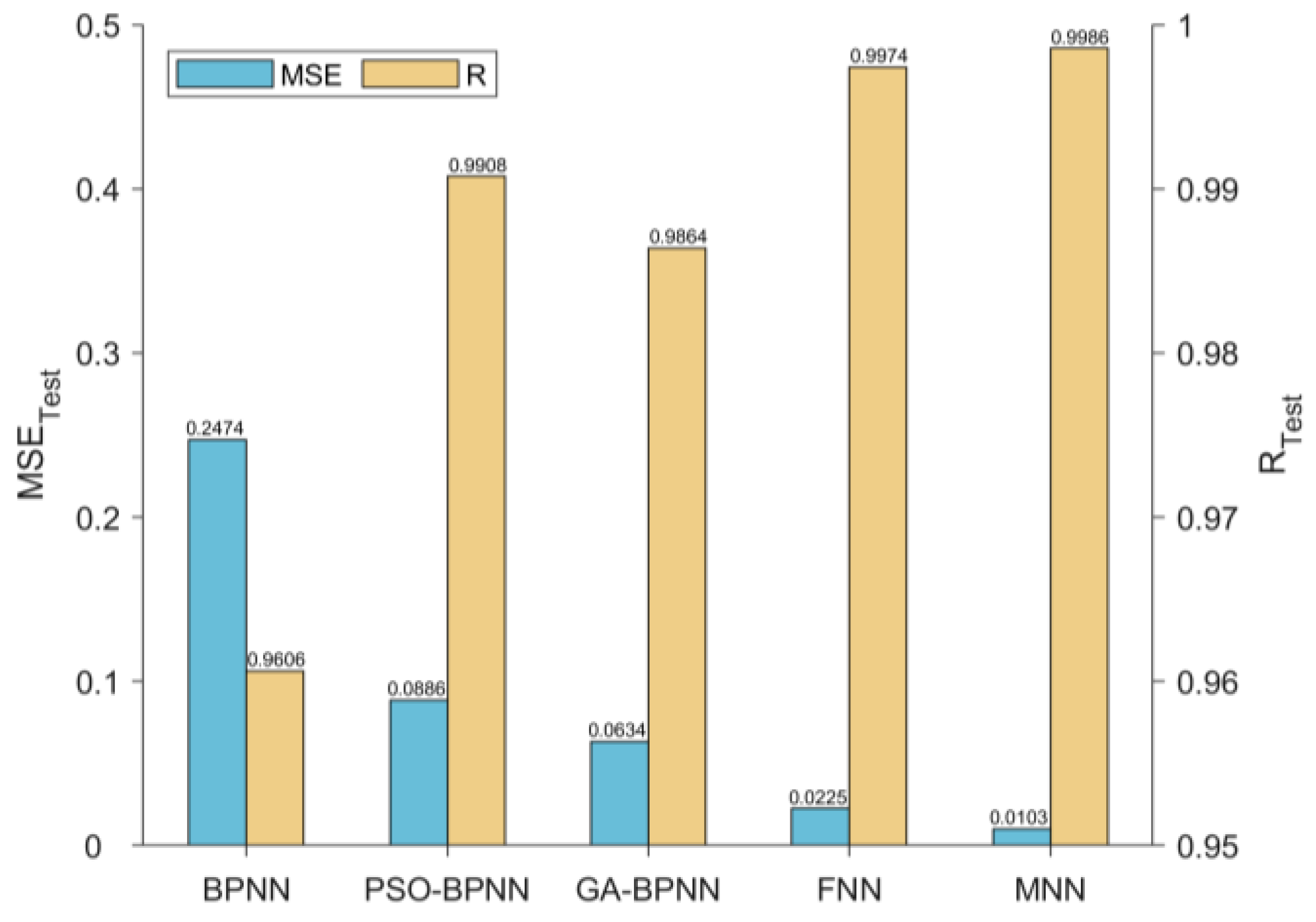
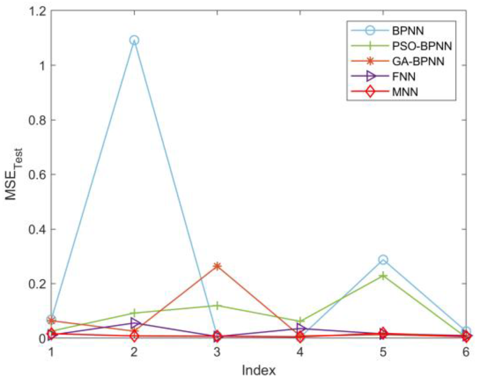
In response to the urgent need for highly accurate and stable intelligent fault diagnosis in spacecraft, this paper proposes an MNN-based intelligent fault diagnosis method for spacecraft fluid loop pumps. The paper also designs software for practical applications and validates the method using both on-orbit telemetry data and ground-based test data. The remainder of this paper is organized as follows. Section 2 introduces the structure and operation principle of the spacecraft fluid loop pump, providing the physical foundation for subsequent analysis. Section 3 describes the proposed intelligent fault diagnosis methodology, including the four base neural network models and the construction of the MNN. 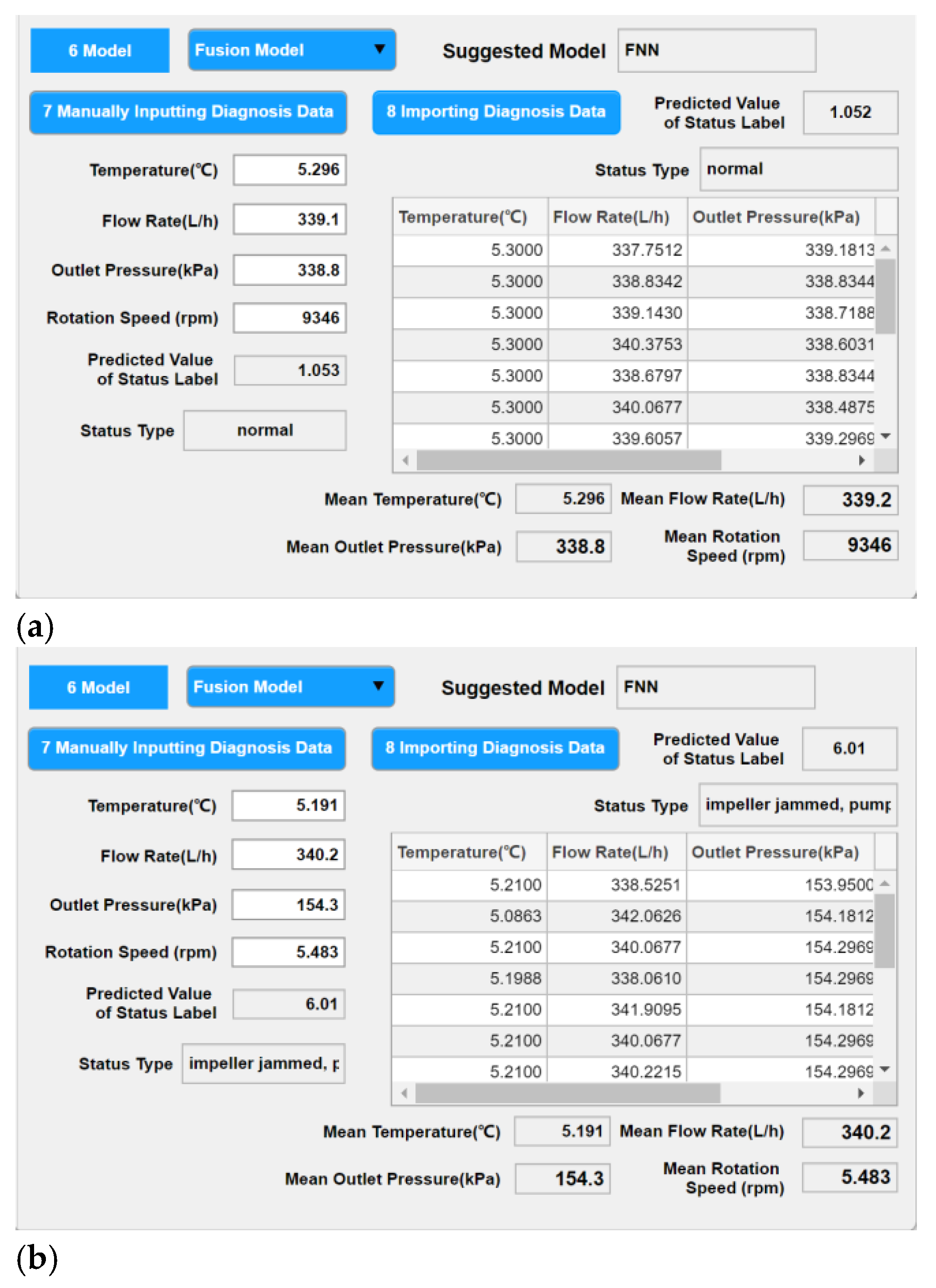Section 4 presents the development and implementation of the intelligent fault diagnosis software. Section 5 validates the proposed method using both on-orbit telemetry data and ground-based test data and includes a detailed parametric and performance analysis. Finally, Section 6 concludes the paper and discusses future research directions.

2. Introduction to Spacecraft Fluid Loop Pumps

Fluid loop pumps are critical components of the spacecraft thermal control system, responsible for maintaining efficient heat transfer within the cabin. The fluid loop system consists of two main circuits: the internal loop and the external loop. In the internal loop, the pump drives the circulation of the working fluid to collect and transport heat generated by onboard equipment. The heat is absorbed through the condenser dryer, which removes moisture and latent heat, and the cold plates, which directly extract heat from electronic devices and thermal loads. The warmed working fluid then passes through an intermediate heat exchanger, where the heat is transferred to the external loop fluid. The external loop includes the propulsion module cold plate and radiators, which ultimately dissipate the absorbed heat into outer space (shown in Figure 1). This closed-loop process enables continuous and precise thermal regulation within the spacecraft cabin, ensuring the stability and reliability of onboard systems [10].

As shown in Figure 2, a spacecraft fluid loop pump is connected to a loop controller, motor, and disconnector. To monitor the performance and health of the pump, it is equipped with outlet pressure sensors, rotational speed sensors, temperature sensors, and flow rate sensors. These sensors continuously provide data on four key status parameters of the fluid loop pump. These parameters serve as the foundational data for fault diagnosis.

3. Intelligent Fault Diagnosis Method

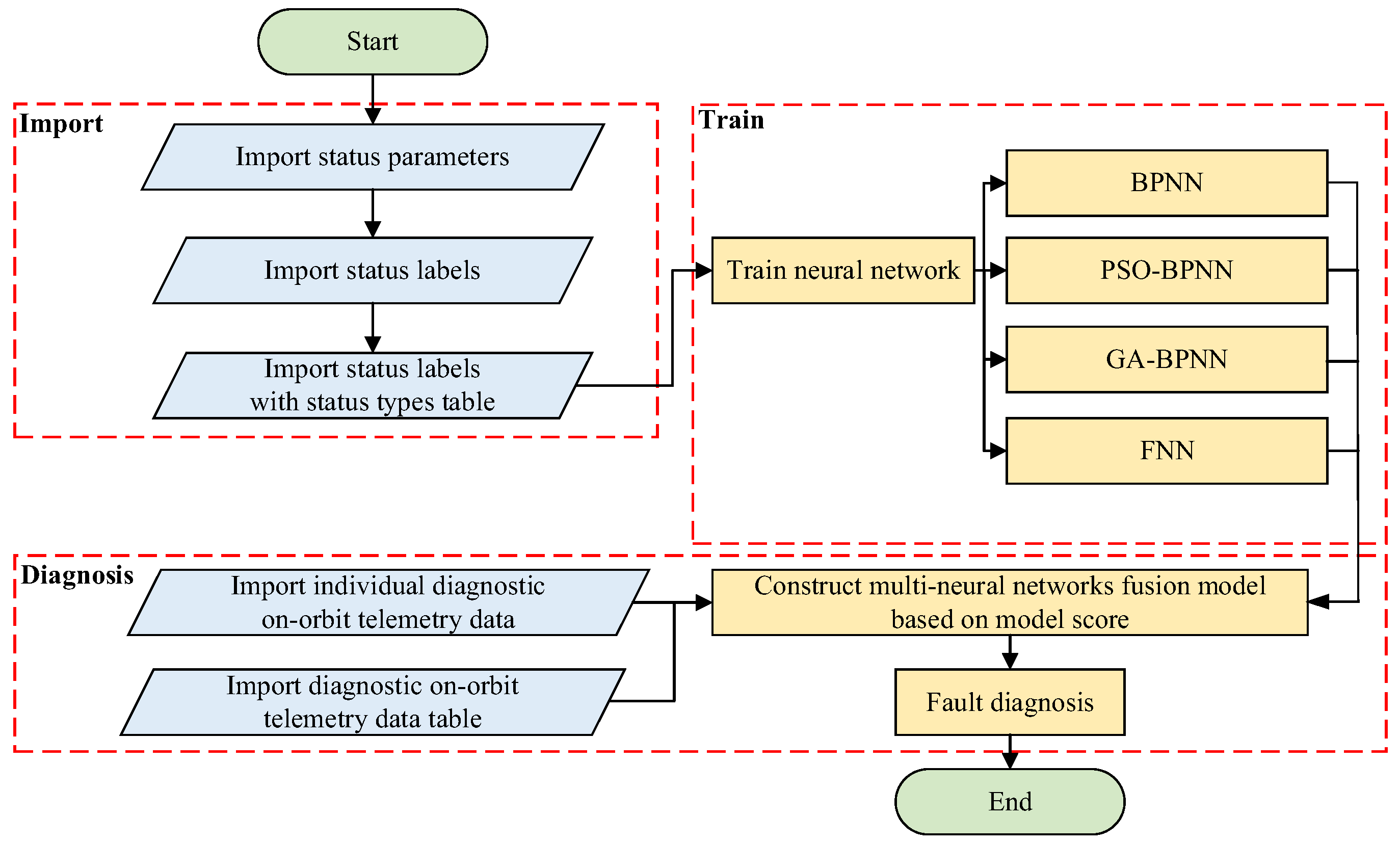
The intelligent fault diagnosis method utilizes the four status parameters of fluid loop pumps as inputs and their corresponding status labels as outputs. Four distinct neural network models are individually trained using this dataset. After the training phase is completed, each model is evaluated to generate a model score. These scores serve as the basis for weighing each model, and the weighted models are then integrated into an MNN. This fusion model is subsequently utilized to diagnose the system data with enhanced accuracy and stability.

3.1. Four Neural Network Models

The structures of these four neural networks are defined by specific model parameters, which are detailed in the “Model Parameter Settings” section. The dataset, comprising the four status parameters and their corresponding status labels for the fluid loop pump, is split into training and test sets. Each neural network is trained independently, taking the status parameters of fluid loop pumps as inputs and generating predicted status labels as outputs.

3.1.1. BPNN Model

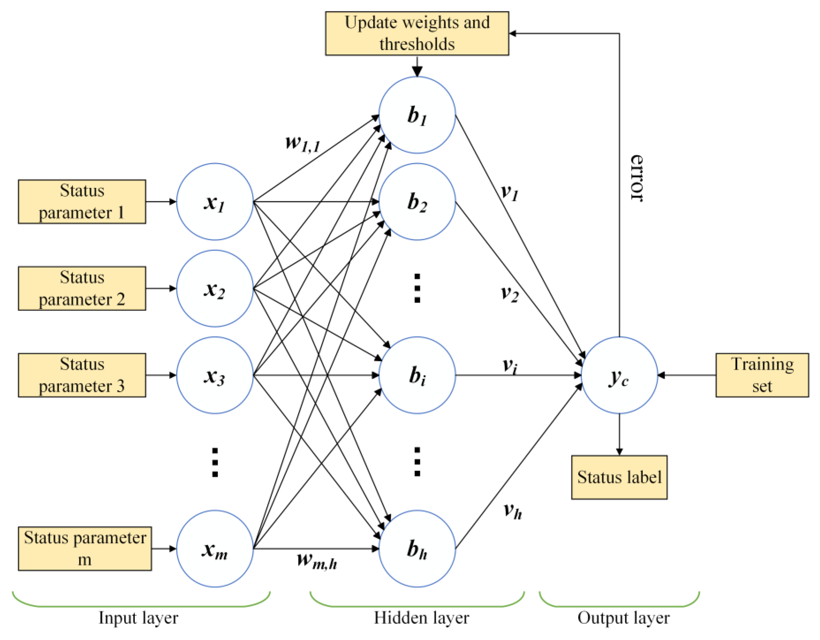
The back propagation neural network (BPNN) is composed of an input layer, a hidden layer, and an output layer. During training, the network iteratively adjusts the weights and thresholds to minimize the discrepancy between the predicted outputs and the actual status labels. Key parameters for constructing a BPNN include the number of neurons in the hidden layer, error threshold, number of iterations, and learning rate. Figure 3 illustrates the BPNN structure used in this study, with the input layer comprising four neurons that represent the fluid loop pump status parameters and the output layer containing one neuron that represents the status label.

The mathematical relationships governing the connections between the input and hidden layers, and between the hidden and output layers, are described by Equations (1) and (2) [29].

$$b_j=f(({\displaystyle \sum _{i=1}^m{x}_i{w}_{j,i}})+{\theta }_j)$$

(1)

$$y_c=f(({\displaystyle \sum _{j=1}^h{b}_j{v}_j})+\beta )$$

(2)

where x_i is the i-th input to input neurons (the i-th status parameter) and m is the number of input neurons; b_j is the j-th input to hidden layer neurons, h is the number of hidden layer neurons, and θ_j is the j-th threshold of hidden layer neurons; w_j,i is the connection weights between the j-th hidden layer neurons and i-th input neurons; f(●) is Sigmoid activation function. While y_c is the prediction value of the neural network, β is the threshold of the prediction value; v_j is the connection weights between the j-th hidden layer neurons and the prediction value of the neural network.

3.1.2. PSO-BPNN Model

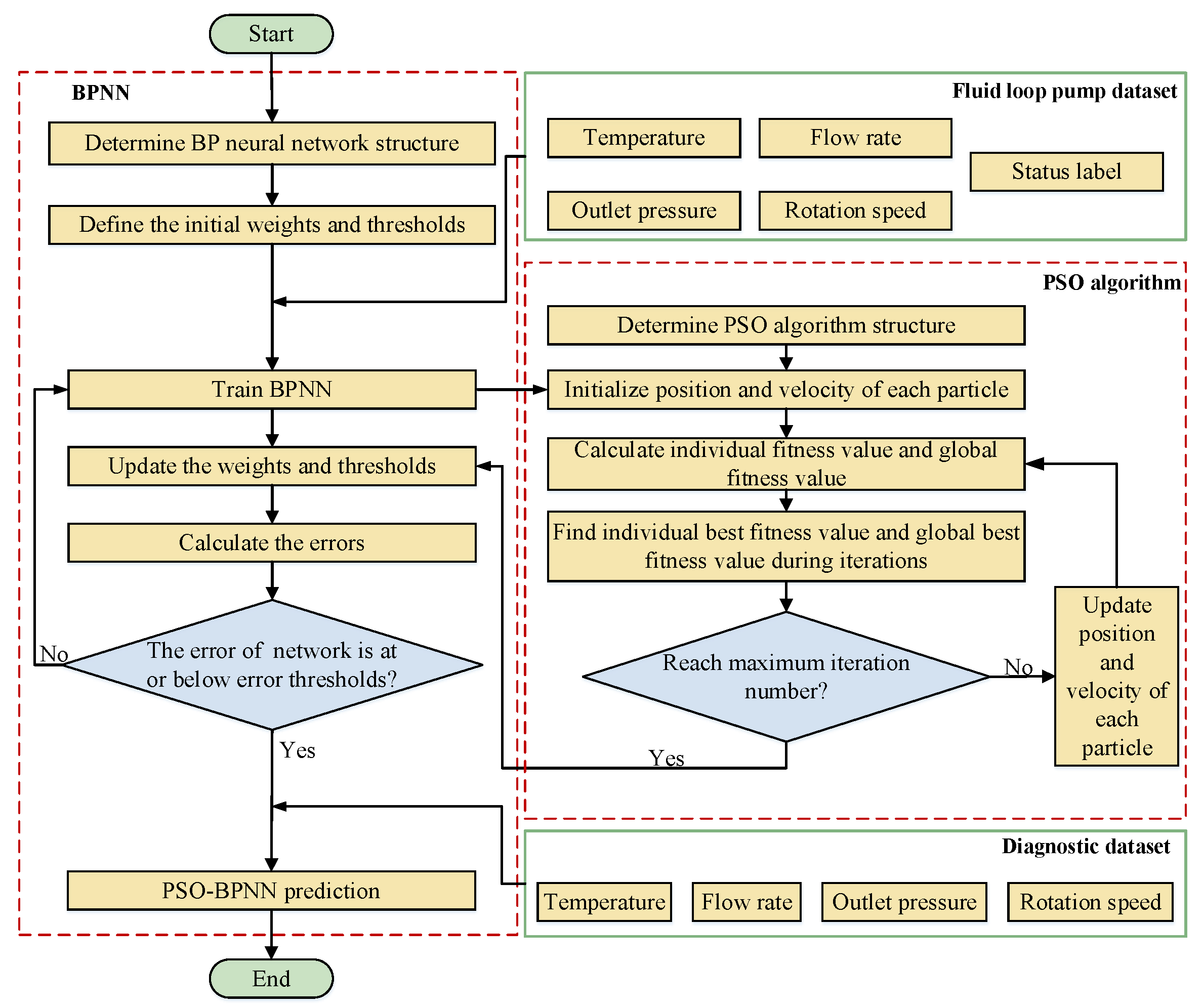
The particle swarm optimization-back propagation neural network (PSO-BPNN) is an enhanced version of the BPNN. It utilizes the particle swarm optimization (PSO) algorithm to optimize the weights and thresholds of the BPNN, thereby improving its performance. This process is illustrated in Figure 4. In the PSO algorithm, each particle represents a potential solution in the solution space for the weights and thresholds of the neural network. By simulating particle velocities and positions, the algorithm aims to find the global optimum while avoiding being trapped in local optima. Key parameters of the PSO algorithm include the learning factor, number of iterations, population size, and the maximum and minimum velocities and positions of particles. The positions and velocities of particles are updated according to Equations (3) and (4) [30].

$$X_j^{\gamma +1}=X_j^{\gamma }+V_j^{\gamma +1}$$

(3)

$$V_j^{\gamma +1}=V_j^{\gamma }+c_1{r}_1\left(p_{best,j}^{\gamma }-X_j^{\gamma }\right)+c_2{r}_2\left(g_{best}^{\gamma }-X_j^{\gamma }\right)$$

(4)

where $X_j^{\gamma }$ is the position of j-th particle in γ-th generation and $V_j^{\gamma }$ is the velocity of j-th particle in γ-th generation; $p_{best,j}^{\gamma }$ is individual best of j-th particle at γ-th iteration and $g_{best}^{\gamma }$ is the global best among γ iterations; c₁ and c₂ are the learning rate factors while r₁ and r₂ are the random numbers.

During the iteration optimization process, the fitness of individual particles and the global fitness are assessed using Equations (5) and (6).

$$f_p^{\gamma }={\displaystyle \frac{1}{n}}{\displaystyle \sum _{j=1}^n{\left(y_{c,j}^{\gamma }-y_{d,j}^{\gamma }\right)}^2}$$

(5)

$$f_g=\min \left(f_p^1,f_p^2,\dots ,f_p^{\gamma },\dots ,f_p^s\right)$$

(6)

where $y_c$${\gamma }_{\gamma d}^{,j}$ is the prediction value of j-th particle in γ-th generation and $y_{\gamma p}^{,j}$ is the actual value of j-th particle in γ-th generation; n is the population size; f is the fitness of γ-th generation and f_g is the global fitness.

3.1.3. GA-BPNN Model

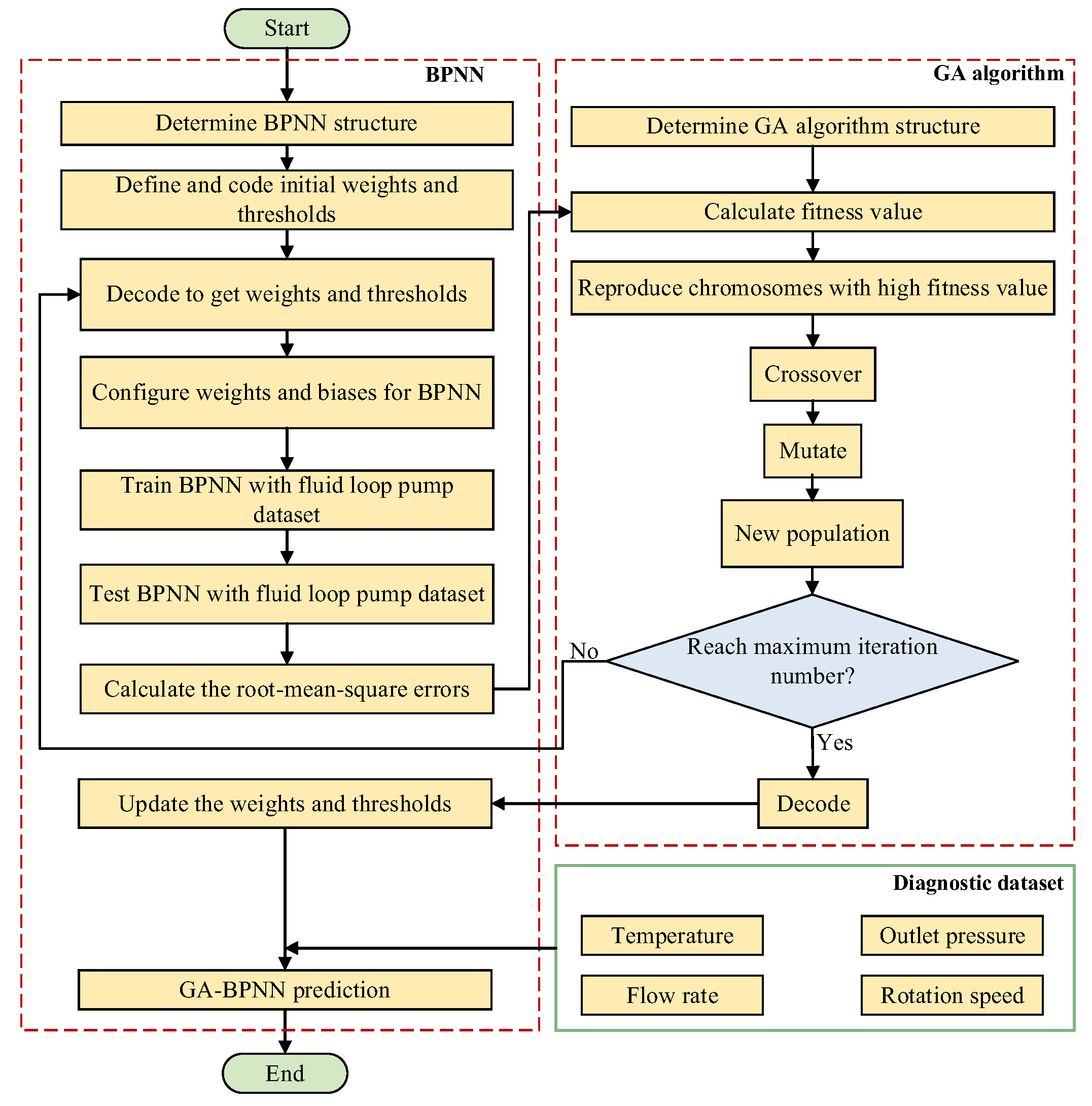
The genetic algorithm-back propagation neural network (GA-BPNN) is also an enhanced variant of the BPNN. It utilizes the genetic algorithm (GA) to optimize the thresholds and weights of the BPNN, as shown in Figure 5. The GA mimics the evolutionary processes of natural populations through selection, crossover, and mutation. It iteratively searches for the optimal initial weights and thresholds of the network, thereby achieving global optimization [31]. In this study, the GA’s performance is fine-tuned by configuring parameters such as the number of generations and population size.

3.1.4. Fuzzy Neural Network Model

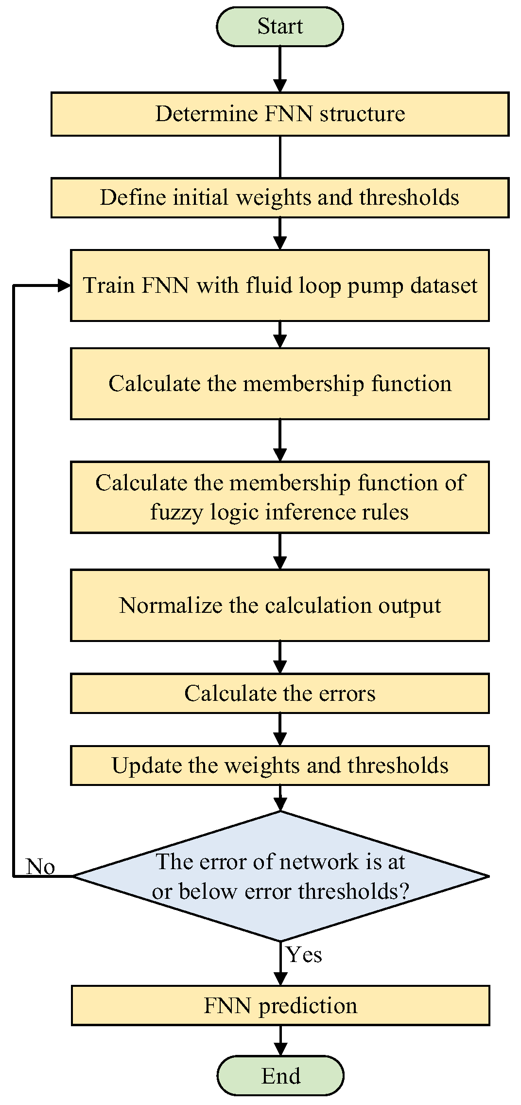
The fuzzy neural network (FNN) integrates fuzzy logic with an artificial feedforward neural network, offering strong self-learning capabilities and efficient direct data processing. The construction process of the FNN is illustrated in Figure 6. Initially, the network structure is established based on the inputs and outputs of the training set. Subsequently, the membership function, network parameters, and the weights and thresholds of the output layer are initialized. The Gaussian function is used for the membership function [32]. The training process involves calculating errors and updating the weights and thresholds iteratively until the error or iteration count meets the predefined termination conditions.

$$A_j^i=\exp [{\displaystyle \frac{-{(x_j-{\mu }_j^i)}^2}{{\sigma }_j^i}}],j=1,2,\dots m,i=1,2,\dots ,l$$

(7)

where $A_j^i$ is the membership function for j-th network input in the i-th fuzzy subset and l is the number of fuzzy subsets; ${\mu }_j^i$ is the center point of the membership function for j-th network input in the i-th fuzzy subset and ${\sigma }_j^i$ is the width of the membership function for the j-th network input in the i-th fuzzy subset.

3.2. Model Evaluation Method

After training the neural network, we need to evaluate its performance by calculating the mean squared error (MSE) M_train and the correlation coefficient (R) R_train between the actual status labels and the predicted values for the training set. Similarly, compute the M_test and R_test for the test set. The MSE and R, as shown in Equations (8) and (9), are chosen as evaluation metrics. It is crucial to minimize the prediction error, measured by the MSE, to accurately identify the operational status of fluid loop pumps. Additionally, a high R ensures that the model’s predictions are reliable and closely aligned with the actual status labels.

$$M={\displaystyle \frac{{\displaystyle \sum _{i=1}^N{(y_{d,i}-y_{c,i})}^2}}{N}}$$

(8)

$$R={\displaystyle \frac{{\displaystyle \sum _{i=1}^N(y_{d,i}-{\overline{y}}_d)(y_{c,i}-{\overline{y}}_c)}}{\sqrt{{\displaystyle \sum _{i=1}^N{(y_{d,i}-{\overline{y}}_d)}^2}}\sqrt{{\displaystyle \sum _{i=1}^N{(y_{d,i}-{\overline{y}}_d)}^2}}}}$$

(9)

To comprehensively evaluate the model’s performance, a scoring mechanism is introduced, which combines the MSE and R from both the training and test sets. Since a higher R and a lower MSE indicate better model performance, the R/MSE ratio is used to integrate these two metrics. Additionally, considering that the MSE is typically much smaller than one, a logarithmic form is adopted to mitigate the significant impact of its minor fluctuations on the results. The training set R_train and M_train are combined with the test sets R_test and M_test in a proportional manner, as shown in Equation (10).

$$S=a\ln ({\displaystyle \frac{R_{train}}{M_{train}}})+(1-a)\ln ({\displaystyle \frac{R_{test}}{M_{test}}})$$

(10)

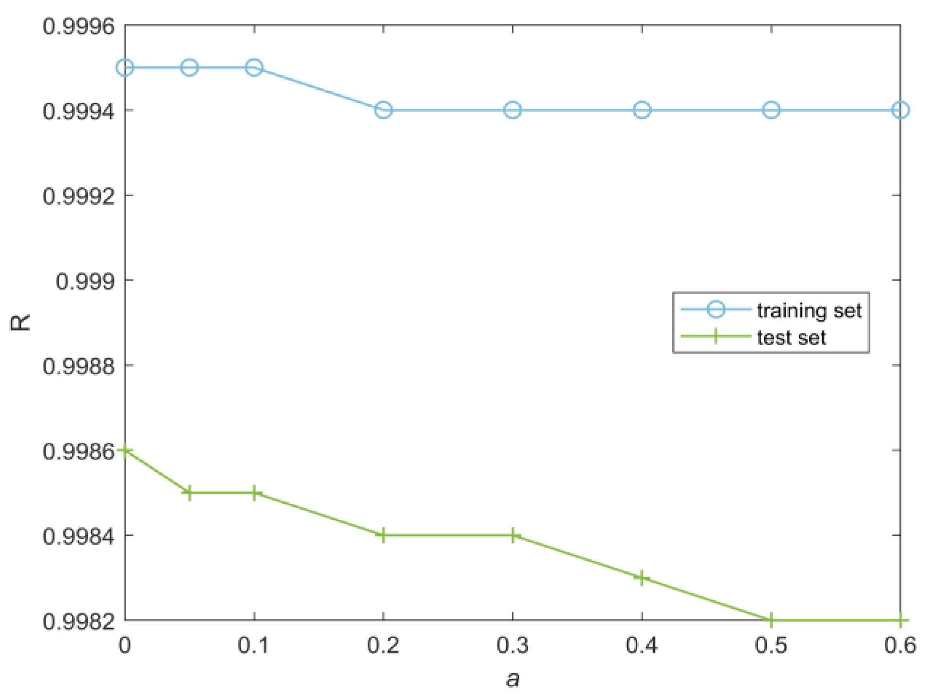
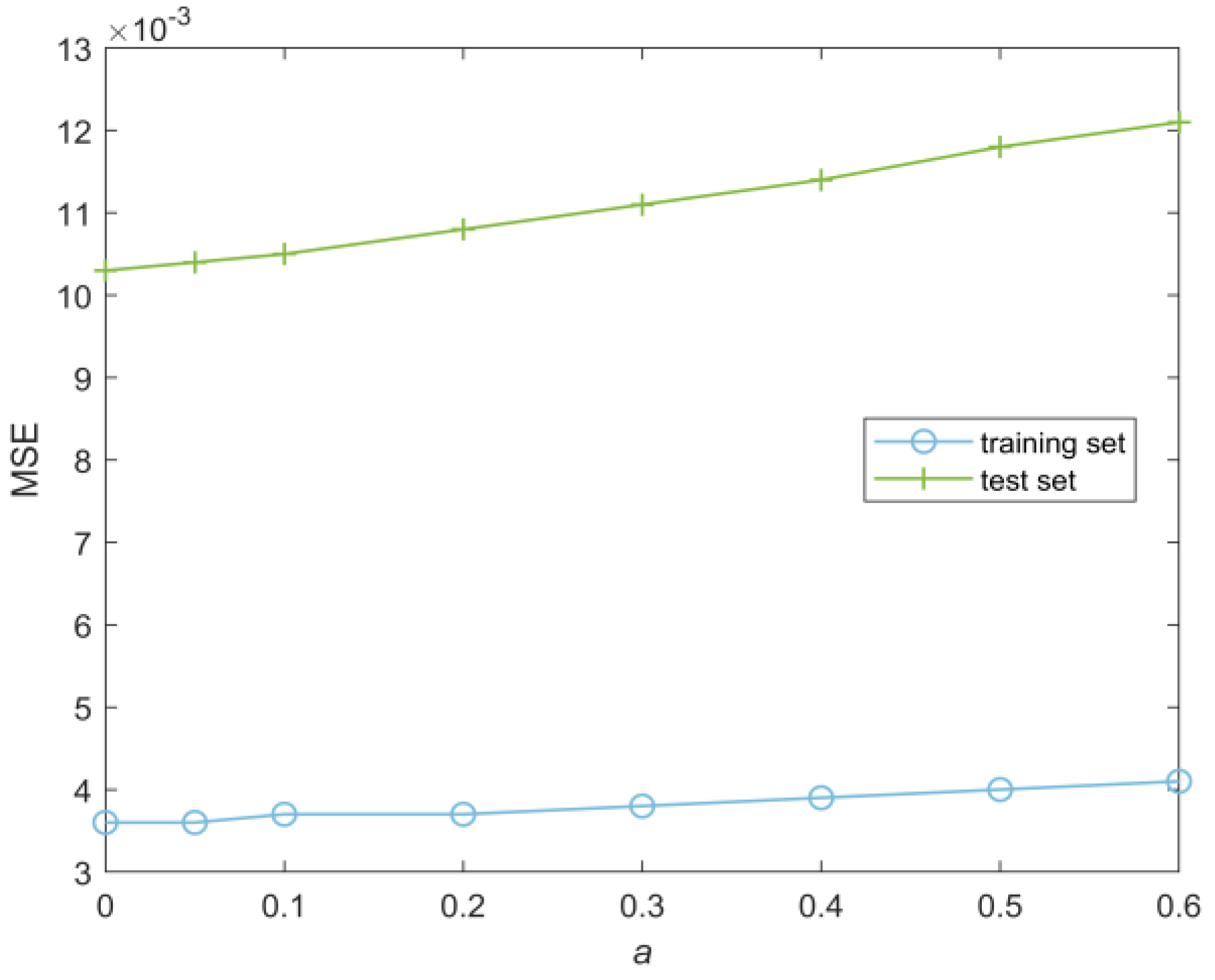
where a (0 ≤ a ≤ 1) represents the weight assigned to the training set performance (including both R_train and M_train) in the scoring formula. Meanwhile, (1 − a) represents the weight assigned to the test set performance (including both R_test and M_test) in the scoring formula. 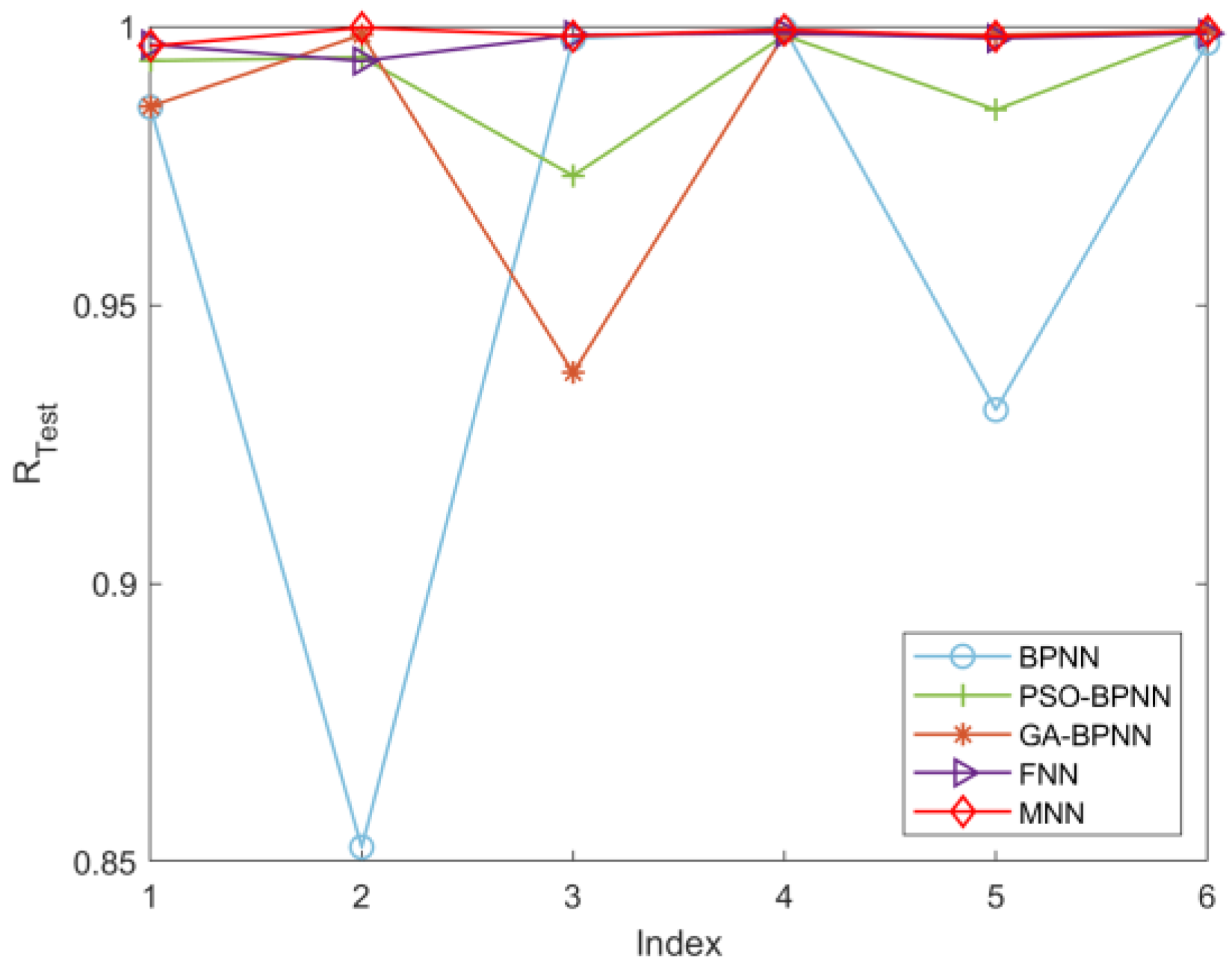The optimal a value will be further determined through k-fold cross-validation to minimize the variance of the test set’s MSE and R, ensuring the model’s stability and generalization ability. A higher model score indicates better training and testing performance. Based on the model scores of the four neural networks, an MNN can be constructed using a weighting algorithm.

To provide a more comprehensive assessment of the model’s diagnostic accuracy, we will also calculate Accuracy, Precision, Recall, and F1-score for the test set. Accuracy measures the proportion of all predictions that are correctly predicted, Precision measures the proportion of true positive predictions among all positive predictions, Recall measures the proportion of true positive predictions among all actual positive instances, and F1-score is the harmonic mean of Precision and Recall, providing a balanced measure of the model’s performance.

3.3. Multi-Neural Network Fusion Model Intelligent Fault Diagnosis Method

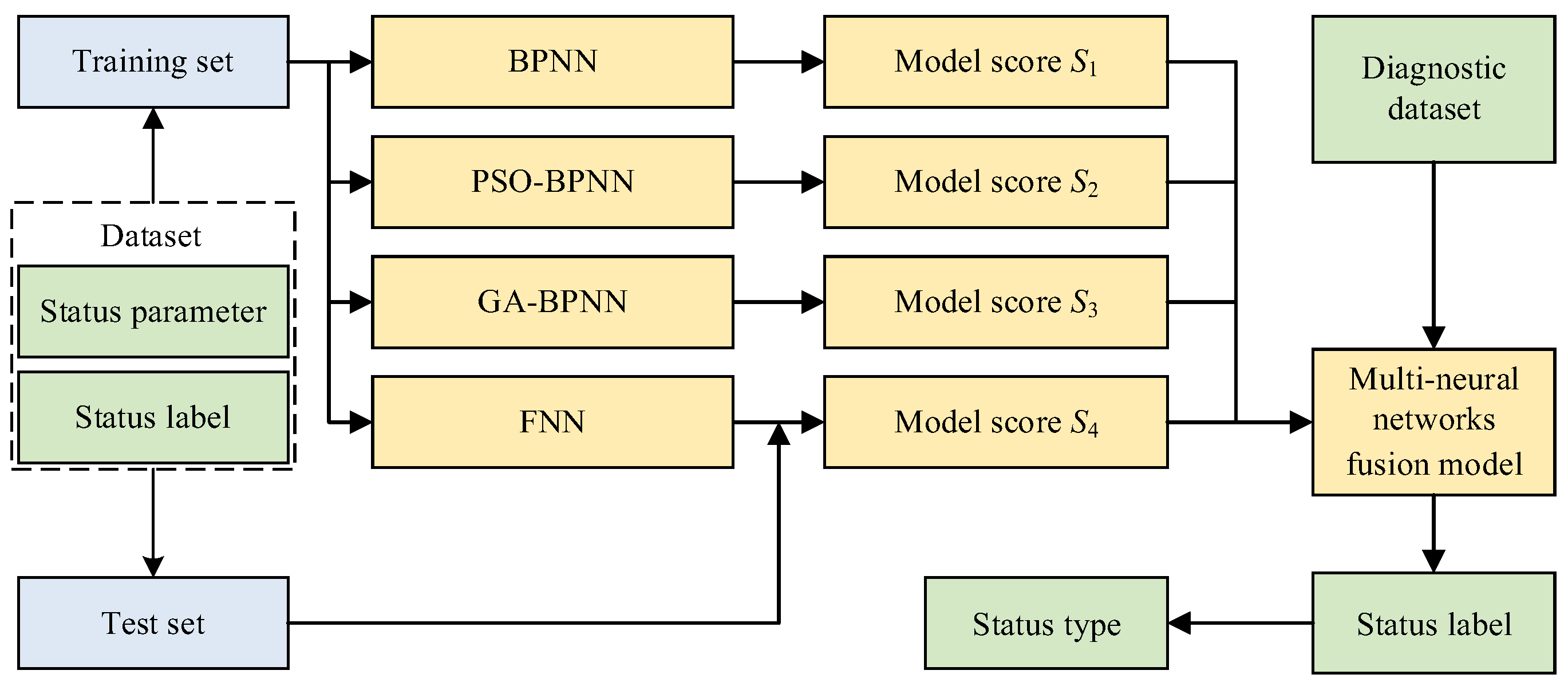
Referring to the flowchart shown in Figure 7, based on the model scores of the four neural networks, the weights for each neural network in the MNN are calculated using Equation (11). The weight W_i of each neural network is proportional to its model score S_i, ensuring that neural networks with higher scores contribute more to the final prediction. The output of the MNN is obtained by taking a weighted sum of the predicted status labels from each neural network, as shown in Equation (12).

$$W_i={\displaystyle \frac{S_i}{{\displaystyle \sum _{i=1}^4{S}_i}}}$$

(11)

$$P_0={\displaystyle \sum _{i=1}^4{W}_i{y}_{c,i}}$$

(12)

This weighted sum allows the fusion model to leverage the strengths of each individual neural network, thereby improving the overall prediction accuracy and stability. The closest integer value p to the predicted value P₀ is taken as the final status label. The status labels are as follows: 1 represents “normal,” 2 represents “slight rubbing between the impeller and pump casing,” 3 represents “severe rubbing between the impeller and pump casing,” 4 represents “fatigue spalling of bearing raceway,” 5 represents “severe fatigue spalling of bearing raceway,” and 6 represents “impeller jammed, pump functionality lost.”

4. Intelligent Fault Diagnosis Software

4.1. Overview of Software Basic Modules

Using the multi-neural network fusion intelligent fault diagnosis method, we have developed intelligent fault diagnosis software for spacecraft fluid loop pumps. As shown in Figure 8, the software features six tabs: (1) Import Data, (2) Train BPNN, (3) Train PSO-BPNN, (4) Train GA-BPNN, (5) Train FNN, and (6) Fault Diagnosis. Each tab is designed to handle specific tasks in the fault diagnosis process, from data import to model training and final diagnosis.

4.2. Software Usage Process

The software utilizes a dataset to train the built-in MNN and diagnose faults. Its functionalities are organized in a sequential manner across the tabs from left to right, as illustrated in Figure 9. The usage procedure consists of three main parts: “Input”, “Training”, and “Diagnosis”.

The “Input” part involves three steps as shown in Figure 10. A dataset, which includes status parameters and status labels, is composed of on-orbit telemetry data and expert experience data. The status parameter table includes four fluid loop pump status parameters: temperature, outlet pressure, flow rate, and rotational speed. The corresponding status label table covers six operating statuses of the fluid loop pumps. Additionally, a status label-to-status type table pairs each status label with its actual status type, enhancing software user-friendliness.

As shown in Figure 11, the “Training” part involves four distinct steps: training the four neural network models and individually evaluating their performance. This process is facilitated through the Train BPNN, Train PSO-BPNN, Train GA-BPNN, and Train FNN tabs, which each include two main areas: one for setting model parameters and another for evaluating model performance. To make better use of the dataset and more accurately evaluate model performance, the software provides a k-fold cross-validation option. Based on the chosen k value, the dataset is randomly divided into k parts, with k iterations performed. In each iteration, k − 1 parts of the data are used as a training set to train the neural networks, while the remaining part serves as a test set. The MSE and R are calculated for each iteration, and the average values of these metrics after k iterations are adopted as the final evaluation metrics.

As shown in Figure 12, the “Diagnosis” part involves two key steps: selecting a model and importing diagnostic data, both of which are accomplished through the Fault Diagnosis tab. In addition to utilizing the MNN, the software also recommends the neural network with the highest model score among the four individual models to diagnose the data.

5. Case Analysis and Application Validation

5.1. Dataset

Neural network training is performed using a dataset comprising status parameters and status labels, sourced from on-orbit data and expert experience. The dataset contains 36 samples listed in

Table 1. Neural network dataset for training and test comprising status parameters and status labels.

Number	Temperature (°C)	Flow Rate (L/h)	Outlet Pressure (kPa)	Rotation Speed (r/min)	Status Label
1	5.30	337.75	339.18	9399.99	1
2	5.30	338.83	338.83	9396.07	1
3	5.30	339.14	338.72	9372.57	1
4	7.30	304.38	328.60	8270.74	2
5	6.90	310.68	330.83	8286.40	2
6	8.30	297.07	322.49	8396.07	2
7	15.30	239.61	239.30	5325.57	3
8	18.30	208.83	209.07	4298.16	3
9	20.30	170.84	180.49	3364.74	3
10	21.30	337.29	330.72	8388.24	4
11	23.28	342.67	329.18	8388.24	4
12	25.29	339.45	318.83	7702.07	4
13	35.29	237.44	238.14	6313.82	5
14	33.29	237.60	219.07	5396.07	5
15	36.30	199.45	178.60	4298.16	5
16	5.17	337.60	153.49	7.83	6
17	5.21	338.99	154.64	3.92	6
18	5.22	338.68	153.49	3.92	6
19	4.80	350.75	342.18	9422.99	1
20	5.00	344.83	344.83	9396.07	1
21	5.10	334.14	335.72	9352.57	1
22	7.80	304.38	328.60	8170.74	2
23	7.40	300.68	310.83	8186.41	2
24	8.80	287.07	312.49	8296.07	2
25	15.30	229.61	220.30	5225.57	3
26	18.80	198.83	209.07	4298.16	3
27	20.80	160.84	180.49	3364.74	3
28	21.80	327.29	330.72	8288.24	4
29	23.08	332.67	322.18	8298.24	4
30	25.79	330.45	308.83	7602.07	4
31	35.89	227.44	228.14	6213.82	5
32	32.09	230.60	210.07	5196.07	5
33	36.80	195.45	173.60	4198.16	5
34	4.57	336.60	155.49	9.83	6
35	5.01	334.99	154.64	4.92	6
36	4.92	342.68	159.49	1.92	6

, each including four status parameters and their corresponding labels, covering six fluid loop pump status types: “normal,” “slight rubbing between the impeller and pump casing,” “severe rubbing between the impeller and pump casing,” “fatigue spalling of bearing raceway,” “severe fatigue spalling of bearing raceway,” and “impeller jammed, pump functionality lost.” The inputs to the neural network are the temperature (°C), flow rate (L/h), outlet pressure (kPa), and rotational speed (r/min) of the fluid loop pump. The flow rate refers to the loop flow rate governed by multiple pumps. Each status label represents a specific status type, serving as the neural network output. The dataset is evaluated using k-fold cross-validation, in which each subset alternately serves as training and test data. Therefore, Table 1 presents the complete dataset, and model performance is reported based on the test folds.

The impeller and motor bearings are key components of the fluid loop pump. When faults occur, the status parameters change in specific ways. For example, improper assembly or an abnormal vibration environment can cause the impeller to rub against the pump casing. This reduces the motor’s rotational speed, leading to a drop in flow rate and outlet pressure. Factors like frictional heat can also cause the fluid temperature to rise. Similarly, an abnormal vibration environment or lubrication failure can lead to bearing raceway fatigue spalling. This increases the bearing’s resistance torque, causing slight reductions in motor speed, flow rate, and outlet pressure. The decreased flow rate also lowers the loop’s heat transfer efficiency, resulting in higher fluid temperatures. Analyzing these fault mechanisms and their impacts helps us understand how the physical failure processes affect pump operation. This, in turn, allows for a more in-depth understanding of the conclusions drawn from the dataset and the data-driven fault diagnosis method.

While we acknowledge that this dataset size is relatively small, it is important to note that the complexity of the fault types and the limited availability of real-world on-orbit telemetry data pose challenges in obtaining a larger dataset. These six types of faults are also recognized as common faults by frontline aerospace experts [32].

5.2. Model Parameter Settings

Import the dataset presented in Table 1 into the spacecraft fluid loop pump intelligent fault diagnosis software. Randomize the dataset and train the four neural networks using six-fold cross-validation. According to experience and the relevant literature [32,33,34], the parameter settings for the four models are detailed in

Table 2. BPNN parameters.

Parameter	Value
Number of hidden layer neurons	8
Maximum number of iterations	1000
Error threshold	1 × 10−6
Learning rate	0.001

,

Table 3. PSO-BPNN parameters.

Parameter	Value
Number of hidden layer neurons	8
Maximum number of iterations	1000
Error threshold	1 × 10−6
Learning rate	0.001
Learning rate factor 1	1.494
Learning rate factor 2	1.494
Number of generations	20
Population size	50
Maximum velocity	1
Minimum velocity	−1
Maximum position	5
Minimum position	−5

,

Table 4. GA-BPNN parameters.

Parameter	Value
Number of hidden layer neurons	8
Maximum number of iterations	1000
Error threshold	1 × 10−6
Learning rate	0.001
Generations	50
Population size	5

and

Table 5. FNN parameters.

Parameter	Value
Number of hidden layer neurons	4
Maximum number of iterations	1 × 104
Error threshold	1 × 10−12
Learning rate	0.075
Network parameter coefficient	0.3
Membership parameter coefficient	0.6

. These values are further verified through preliminary experiments to ensure stable convergence and reliable diagnostic performance. Given the large number of parameters and the diversity of network types, only the general parameter selection principles are presented here for clarity.

5.3. Discussion on Coefficient a

Referring to

Table 6. R, MSE, and their variances of the multi-neural network fusion model with changes in a.

a	Rtrain	Rtest	Mtrain	Mtest	Variance of Rtest	Variance of Mtest
0	0.9995	0.9986	0.0036	0.0103	7.0607 × 10−6	1.58 × 10−4
0.05	0.9995	0.9985	0.0036	0.0104	7.5136 × 10−6	1.69 × 10−4
0.1	0.9995	0.9985	0.0037	0.0105	7.9589 × 10−6	1.80 × 10−4
0.2	0.9994	0.9984	0.0037	0.0108	8.8259 × 10−6	2.03 × 10−4
0.3	0.9994	0.9984	0.0038	0.0111	9.6614 × 10−6	2.26 × 10−4
0.4	0.9994	0.9983	0.0039	0.0114	1.0467 × 10−5	2.47 × 10−4
0.5	0.9994	0.9982	0.0040	0.0118	1.1245 × 10−5	2.68 × 10−4
0.6	0.9994	0.9982	0.0041	0.0121	1.1997 × 10−5	2.88 × 10−4

, the coefficient a has a significant impact on R, MSE, and their variances of the MNN. The R and MSE presented here are the mean values obtained from six-fold cross-validation, with the variances calculated from the six iterations. It can be observed that when a is 0, both R_train and R_test reach their maximum values, while M_train and M_test are minimized. Additionally, the variances of R_test and M_test are also the smallest. At this point, the model achieves optimal predictive performance and stability.

The correlation coefficient and mean squared error of the MNN as functions of a are shown in Figure 13 and Figure 14. As a increases from 0 to 0.6, the correlation coefficients R_train and R_test gradually decrease, while M_train and M_test increase approximately linearly. The closer a is to 0, the smaller the weight assigned to the training set and the larger the weight assigned to the test set in Equation (10), the better the prediction performance of the MNN. Combining this with the analysis results in Table 6, the optimal model is achieved when a is 0. At this point, the model performance is entirely determined by the test set correlation coefficient and mean squared error, independent of the training set. Equation (10) can thus be simplified to the following:

$$S=\ln ({\displaystyle \frac{R_{test}}{M_{test}}})$$

(13)

5.4. Performance and Stability Analysis of Neural Networks

As shown in Figure 15, the average values of the MSE and R for the test set are calculated after six-fold cross-validation. When the coefficient a = 0, the MNN demonstrates the best predictive performance. Specifically, it achieves a test set R of 0.9986, outperforming the four individual neural networks. Moreover, it has the lowest test set MSE of 0.0103 among the five models.

As illustrated in

Table 7. Performance comparison of multi-neural network fusion model with four neural networks.

	Mtest	Reduction in Mtest	Rtest	Increase in Rtest
MNN	0.0103	/	0.9986	/
BPNN	0.2474	95.84%	0.9606	3.96%
PSO-BPNN	0.0886	88.37%	0.9908	0.79%
GA-BPNN	0.0634	83.75%	0.9864	1.24%
FNN	0.0225	54.22%	0.9974	0.01%

, the MNN significantly enhances performance compared to the four individual neural networks. Specifically, when compared with BPNN, PSO-BPNN, GA-BPNN, and FNN, its MSE is reduced by 95.84%, 88.37%, 83.75%, and 54.22%, respectively, while the R value remains relatively constant.

In terms of neural network stability, the variances of the MSE and R during six-fold cross-validation serve as the evaluation metrics. Figure 16 and Figure 17 show that the MNN experiences minimal fluctuations in both MSE and R across the six iterations, indicating its superior stability across diverse training and test sets. Notably, the variance of MSE in the test set as low as 0.0002, while the variance of R is 0.00001.

Table 8. Stability comparison of multi-neural network fusion model with four neural networks.

	Variance of MSE	Reduction in Variance of MSE	Variance of R	Reduction in Variance of R
MNN	0.0002	/	0.00001	/
BPNN	0.9133	99.97%	0.01740	99.94%
PSO-BPNN	0.0326	99.39%	0.00051	98.03%
GA-BPNN	0.0505	99.60%	0.00300	99.67%
FNN	0.0019	89.47%	0.00002	50.00%

displays a stability comparison of MNN with four neural networks. Specifically, the fusion model reduces the variance of MSE by 99.97%, 99.39%, 99.60%, and 89.47%, and the variance of R by 99.94%, 98.03%, 99.67%, and 50.00% when compared to the BPNN, PSO-BPNN, GA-BPNN, and FNN, respectively. These results confirm that the stability of the fusion model is significantly improved compared with the other four models.

In addition to MSE and R, we compared the Accuracy, Precision, Recall, and F1-score of the MNN against four individual neural networks on the test set. It is worth noting that while the MNN and FNN demonstrated identical performance in terms of Accuracy, Precision, Recall, and F1-score, the MNN exhibited superior performance in MSE and R. Specifically, the MNN and FNN both achieved perfect scores of 1.000 for Accuracy, Precision, Recall, and F1-score. In comparison, the BPNN model has an Accuracy of 0.954, Precision of 0.846, Recall of 0.862, and an F1-score of 0.851; the PSO-BPNN model has an Accuracy of 0.972, Precision of 0.938, Recall of 0.917, and an F1-score of 0.926; the GA-BPNN model has an Accuracy of 0.961, Precision of 0.914, Recall of 0.942, and an F1-score of 0.926. These results underscore the MNN’s diagnostic accuracy, which is further validated by the fact that the Accuracy, Precision, Recall, and F1-score values are obtained through k-fold cross-validation (k = 6), ensuring their reliability and generalizability. Equations (14)–(17) illustrate the formulas used to calculate these metrics on the test set.

$$Accurac{y}_{test}={\displaystyle \frac{1}{k}}{\displaystyle \sum _{i=1}^k\left[\frac{1}{6}{\displaystyle \sum _{j=1}^6\left(\frac{T{P}_{ij}+T{N}_{ij}}{T{P}_{ij}+F{P}_{ij}+F{N}_{ij}+T{N}_{ij}}\right)}\right]}$$

(14)

$$Precisio{n}_{test}={\displaystyle \frac{1}{k}}{\displaystyle \sum _{i=1}^k\left[\frac{1}{6}{\displaystyle \sum _{j=1}^6\left(\frac{T{P}_{ij}}{T{P}_{ij}+F{P}_{ij}}\right)}\right]}$$

(15)

$${Recall}_{test}={\displaystyle \frac{1}{k}}{\displaystyle \sum _{i=1}^k\left[\frac{1}{6}{\displaystyle \sum _{j=1}^6\left(\frac{T{P}_{ij}}{T{P}_{ij}+F{N}_{ij}}\right)}\right]}$$

(16)

$$F_1-{score}_{test}={\displaystyle \frac{1}{k}}{\displaystyle \sum _{i=1}^k\left(\frac{{2Precision}_i·{Recall}_i}{{Precision}_i+{Recall}_i}\right)}$$

(17)

5.5. Application Verification Based on On-Orbit Telemetry Data

To verify the functionality of the MNN, it is selected within the spacecraft fluid loop pump intelligent fault diagnosis software to perform fault diagnosis using on-orbit telemetry data under two different status types. The diagnosis is conducted based on two representative segments of steady-state telemetry data extracted from a large amount of on-orbit data to ensure reliability and typicality.

First, the on-orbit telemetry data for a fluid loop pump under normal status is imported, as shown in

Table 9. On-orbit telemetry data of fluid loop pump under “normal” status.

Temperature (°C)	Flow Rate (L/h)	Outlet Pressure (kPa)	Rotation Speed (r/min)
5.30	337.75	339.18	9399.99
5.30	338.83	338.83	9396.07
5.30	339.14	338.72	9372.57
5.30	340.38	338.60	9270.74
5.30	338.68	338.83	9286.41
5.30	340.07	338.49	9396.07
5.30	339.61	339.30	9325.57
5.30	338.83	339.07	9298.16

. As illustrated in Figure 18a, the software calculates the mean values of the four status parameters and performs a fault diagnosis. The result indicates “normal,” which aligns with the actual on-orbit status of the fluid loop pump.

Next, the on-orbit telemetry data for a fluid loop pump under fault status is imported, as shown in

Table 10. On-orbit telemetry data of fluid loop pump under “impeller jammed” status.

Temperature (°C)	Flow Rate (L/h)	Outlet Pressure (kPa)	Rotation Speed (r/min)
5.21	338.53	153.95	3.92
5.09	342.06	154.18	7.83
5.21	340.07	154.30	3.92
5.20	338.06	154.30	7.83
5.21	341.91	154.18	3.92
5.21	340.07	154.30	3.92
5.21	340.22	154.30	3.92
5.21	337.75	154.53	3.92

, with a specific fault “impeller jammed.” As illustrated in Figure 18b, the software calculates the mean values of the four status parameters and performs a fault diagnosis. The result indicates “impeller jammed, pump functionality lost,” which accurately reflects the actual on-orbit status of the fluid loop pump.

5.6. Application Verification Based on Ground Test Data

Referring to Figure 19, to further validate the MNN, a 6200 bearing test specimen with a simulated “fatigue spalling of bearing raceway” fault is manufactured. The simulated defect is located on the outer race of the fluid loop pump bearing, with dimensions of approximately 1.10 mm × 0.49 mm.

The 6200 faulty bearing is installed into the ground test facility for the fluid loop pump, as shown in Figure 20. The positions of the sensors in the ground test facility are consistent with those in the on-orbit configuration, including the outlet pressure sensor, rotational speed sensor, temperature sensor, and flow rate sensor. After stable operation for about 0.5 h, the mean values of the steady-state temperature, flow rate, outlet pressure, and rotational speed are measured to be 25.56 °C, 306.4 L/h, 300.9 kPa, and 8849 r/min, respectively.

As shown in Figure 21, when this data is imported into the software, the fault diagnosis result is identified as “fatigue spalling of bearing raceway,” which matches the actual fault type.

6. Conclusions

To address the high failure rate of the spacecraft thermal control subsystem, particularly fluid loop pumps, and the low stability of predictions from individual neural network models, this paper proposes an intelligent fault diagnosis method based on an MNN. This method provides an effective solution for diagnosing faults in spacecraft fluid loop pumps and is expected to play a crucial role in the intelligent maintenance of spacecraft. The main conclusions are as follows:

(1)

The MNN significantly outperforms the four individual neural networks it integrates. Using the fluid loop pump dataset, the MNN achieved a test set R of 0.9986 and an MSE of 0.0103, demonstrating excellent predictive performance. Compared to the BPNN, PSO-BPNN, GA-BPNN, and FNN, the MNN, respectively, reduced the MSE by 95.84%, 88.37%, 83.75%, and 54.22%.

(2)

The MNN demonstrates superior stability across various training and test sets compared to the individual models. The model has improved the stability of the individual models with the reduction in the MSE variance by 99.97%, 99.39%, 99.60%, and 89.47% and the reduction in the R variance by 99.94%, 98.03%, 99.67%, and 50.00%, respectively.

(3)

In addition to MSE and R, the MNN also demonstrated superior diagnostic accuracy in terms of Accuracy, Precision, Recall, and F1-score, achieving perfect scores of 1.000 for these metrics. These results are obtained through six-fold cross-validation, ensuring their reliability and generalizability.

(4)

An intelligent fault diagnosis software for spacecraft fluid loop pumps has been developed based on the proposed method. Validation with both on-orbit telemetry data and ground test data demonstrates that the software accurately identifies both normal and faulty statuses. Specifically, the software not only correctly diagnosed the normal operation and impeller jammed faults in on-orbit telemetry data but also accurately identified a simulated “fatigue spalling of bearing raceway” fault in ground test data. The accurate diagnostic results obtained from these three datasets demonstrate the robustness and generalization capability of the proposed method under different operating conditions. While the proposed intelligent fault diagnosis method shows promise, it has certain limitations, such as a limited range of identifiable status types and insufficient integration of knowledge and space-ground data.