A Reformulated-Vortex-Particle-Method-Based Aerodynamic Multi-Objective Design Optimization Strategy for Proprotor in Hover and High-Altitude Cruise

Abstract

An improved multi-objective design optimization framework is proposed for the efficient design of proprotor blades tailored to specific high-altitude mission requirements. This framework builds upon existing methods by leveraging a reformulated Vortex Particle Method (rVPM) and incorporates three key stages: (1) rapid determination of overall proprotor parameters using a semi-empirical model, (2) optimized blade chord and twist distribution bounds based on minimum energy loss theory, and (3) global optimization with a high-fidelity rVPM-based aerodynamic solver coupled with a multi-objective hybrid optimization algorithm. Applied to a small high-altitude tiltrotor, the framework produced Pareto-optimal proprotor designs with a figure of merit of 0.814 and cruise efficiency of 0.896, exceeding mission targets by over 15%. Key findings indicate that large taper ratios and low twist improve hover performance, while elliptical blade planforms with high twist enhance cruise efficiency, and a tip anhedral further boosts overall performance. This framework streamlines the industrial customization of proprotor blades, significantly reducing the design space for advanced optimization while improving performance in demanding high-altitude environments.

1. Introduction

Tiltrotors, combining the vertical take-off and landing (VTOL) and hovering capabilities of helicopters with the high-speed cruise performance of fixed-wing aircraft, represent a versatile platform with broad applications. This unique blend of attributes has garnered significant attention from aerospace researchers [1]. Increasing demand for high-altitude unmanned aerial vehicles (UAVs), particularly for reconnaissance, search, and rescue missions in both military and civilian sectors, has further cemented tiltrotors as a preferred solution [2].

The aerodynamic design of proprotors is crucial for achieving optimal performance in both hover and cruise conditions, particularly at high altitudes where low air density significantly affects aerodynamic efficiency. Mainstream rotor aerodynamic models typically fall into three categories. The Blade Element Momentum Theory (BEMT) model [3], renowned for its computational efficiency and reasonable accuracy in predicting conventional rotor performance, faces limitations when dealing with more complex geometries and in low-density environments. Vortex-based wake models, including the free wake model [4] and the vortex particle model [5], strike a balance between accuracy and computational efficiency. Lastly, the grid-based Computational Fluid Dynamics (CFD) [6] approach provides the highest accuracy but at the cost of significant computational resources. Studies such as those on the XV-15 rotor [7] have extensively validated CFD, which, when combined with Computational Structural Dynamics (CSD), can achieve high-fidelity predictions of rotor loads and deformations [8].

Research into the V-22 tiltrotor’s rotor blades has driven significant advancements in proprotor design. Farrell’s multi-objective optimization work [9] and Rosenstein’s comprehensive analysis of aerodynamic components [10] have been particularly influential. Rosenstein’s work demonstrated notable improvements in rotor efficiency and reduced interference, surpassing the performance of the XV-15 rotor in both hover and cruise through wind tunnel testing and theoretical validation.

Proprotor design for high-altitude UAVs faces substantial challenges due to conflicting hover and cruise performance requirements, as well as the reduced air density at high altitudes [11]. To perform optimally, proprotors must achieve a high figure of merit ($FM$) in standard atmospheric conditions ($\rho =1.225{\mathrm{kg}/\mathrm{m}}^3$) [12] while maintaining high propulsive efficiency during high-speed cruise in low-density environments, such as 4500 m above sea level ($\rho =0.78{\mathrm{kg}/\mathrm{m}}^3$) [13]. Hover performance benefits from increased blade radius and tip speed, while cruise performance is enhanced by reducing rotational speed or blade radius to minimize drag. Moreover, blade twist plays a critical role; smaller twist angles improve hover by increasing lift at low forward speeds, while larger twist angles enhance cruise efficiency by reducing drag and optimizing lift distribution along the blade span. These conflicting design requirements are further complicated by the varying atmospheric densities across the operating envelope, making the optimization process heavily reliant on iterative design–test cycles [14].

Recent advancements in active rotor technologies—such as adaptive rotor diameters [15], active blade rotational speed/twist control [16], and active blade tip control [17]—show potential for resolving these conflicting requirements through dynamic optimization of proprotor blade profiles. However, practical implementation remains hindered by mechanical complexities and structural limitations.

Thus, multi-objective optimization techniques that address the conflicting aerodynamic requirements of proprotor blades across varying flight conditions are critical. In addition to selecting chord, twist, and airfoil distributions, other factors such as the blade tip anhedral [18] and sweep [19] play important roles in optimizing rotor performance in different flight modes [20]. While aeroelastic effects and blade deformations are crucial factors in rotor design [21], this study focuses primarily on axial flow optimization, leaving these effects for future research.

Further, recent research has emphasized the need to integrate both aerodynamic and structural models in proprotor optimization. Hoyos et al. [22], for example, developed an aero-structural optimization method that combines BEMT and particle swarm optimization, yielding higher thrust and efficiency by carefully considering both aerodynamic and structural constraints. Although this paper focuses on aerodynamic optimization, future work will consider incorporating structural models to evaluate their impact on design.

Several previous studies have successfully applied optimization techniques to various rotorcraft configurations, such as tiltrotors and compound helicopters. Yeo and Johnson [23] employed a multidisciplinary approach, combining Lifting-Line Methods with optimization to balance hover and cruise performance. Droandi et al. [24] developed a two-layer optimization framework combining BEMT with CFD, while Hwang and Ning [25] focused on optimizing cruise and high-lift propellers for NASA’s X-57 aircraft, showing significant performance improvements [26,27]. Despite the comprehensive nature of CFD-based optimization [28], its high computational cost [29] has led to the adoption of surrogate or low-fidelity models to achieve a balance between efficiency and accuracy [30,31].

Sridharan and Sinsay [32] proposed a multi-fidelity optimization framework that employs surrogate models like Gaussian Processes and neural networks to enhance the efficiency and accuracy of rotor aerodynamic design. Similarly, Cornelius and Schmitz [33] introduced a machine-learning-based approach to optimize rotor designs with reduced computational costs while maintaining high fidelity. Anusonti-Inthra [34] applied an orthogonal CST method combined with surrogate modeling to improve airfoil parameterization, which has promising applications in rotorcraft optimization. While surrogate models allow for high-precision rotor design optimization, their development requires extensive high-fidelity sampling, which incurs significant computational costs. Moreover, optimization outcomes using surrogate models may not always align with results obtained from metamodels. Thus, incorporating models with greater computational efficiency remains practically valuable, provided that fidelity is maintained.

Nonetheless, many optimization frameworks still rely on baseline blade shapes, limiting convergence when applied to varied design objectives. To address this, Zhang et al. [35] proposed a general framework combining BEMT models with high-fidelity CFD for validation, but reliance on low-fidelity models during the optimization phase can still lead to deviations from the true optimal solution.

In this paper, we extend previous research by developing an improved multi-objective optimization framework for proprotor blades, specifically targeting performance in hover and high-altitude cruise conditions. This improved framework offers a generalized method for determining key proprotor parameters, such as the number of blades, rotational speed, and solidity, which are critical for meeting mission-specific performance targets, particularly at high altitudes. Based on these parameters, ideal bounds for chord and twist distributions are established to ensure a balanced performance between hover and cruise efficiency. Airfoil distributions along the blade span are carefully selected to optimize aerodynamic performance across various flight conditions, including those encountered at high altitudes.

A high-fidelity simulation tool based on the reformulated Vortex Particle Method (rVPM) [36,37,38] is employed to compute the figure of merit ($FM$) for hover and the cruise efficiency ($\eta$). The rVPM model accurately handles complex flow phenomena, such as blade–vortex interactions, while remaining computationally efficient. These aerodynamic models are then coupled with a many-objective hybrid optimizer (MOHO), dynamically selecting optimization algorithms based on real-time performance during the search process. This approach allows for rapid convergence to Pareto-optimal blade configurations that simultaneously optimize both hover and cruise efficiency. The resulting optimized designs achieve a hover efficiency of $FM\approx 0.814$ and a cruise efficiency of $\eta \approx 0.896$, exceeding mission requirements and demonstrating the effectiveness of this optimization strategy.

2. Numerical Methodology

2.1. Rapid Estimation Model for Overall Parameters

This study initially constructs semi-empirical estimation models for hover efficiency and high-altitude cruise propulsive efficiency. These models are then integrated with the classical Nelder–Mead efficient optimization algorithm [39] to expeditiously determine the overall parameters of the high-altitude tiltrotor, encompassing rotor diameter (D), solidity ($\sigma$), and rotor speed ($\Omega$).

Based on Glauert’s momentum theory, the ideal induced inflow ratio of the hovering rotor ${\lambda }_h$ is given by the following:

$${\lambda }_h={\displaystyle \frac{\sqrt{T/\left(2\rho A\right)}}{\Omega R}}=\sqrt{C_T/2}$$

(1)

where T represents the rotor thrust, $C_T=T/\rho \pi R^2{(\Omega R)}^2$ represents the thrust coefficient, $\rho$ denotes the air density, $A=\pi R^2$ signifies the rotor disk area, and $R=D/2$ is the rotor radius.

For pure axial flow conditions, the estimation formula for the inflow ratio [40] is expressed as follows:

$$\lambda =\left\{\begin{array}{cc}{\displaystyle \frac{{\mu }_z}{2}}+s\sqrt{{\left({\displaystyle \frac{{\mu }_z}{2}}\right)}^2+{\lambda }_h^2}\hfill & -{\lambda }_h<s{\mu }_z\hfill \\ {\mu }_z\left[{\displaystyle \frac{0.373{\mu }_z^2}{{\lambda }_h^2}}-0.991\right]\hfill & -2{\lambda }_h<s{\mu }_z<-{\lambda }_h\hfill \\ {\displaystyle \frac{{\mu }_z}{2}}-s\sqrt{{\left({\displaystyle \frac{{\mu }_z}{2}}\right)}^2-{\lambda }_h^2}\hfill & s{\mu }_z<-2{\lambda }_h\hfill \end{array}\right.$$

(2)

where ${\mu }_z$ denotes the axial component of the advance ratio (for pure axial flow, ${\mu }_z=V_f/V_{tip}$), $V_f$ is the axial freestream velocity, $V_{tip}=\Omega R$ is the rotor tip speed, and $s=sign{C}_T$.

The Newton–Raphson method, with appropriate relaxation factors to enhance convergence, is employed to solve the iterative process of induced velocity. In this study, a relaxation factor of 0.5 is determined to be optimal, with calculations converging in three to four iterations.

Rotor power is composed of induced power, profile power, interference power, and parasite drag power. This study focuses primarily on induced and profile power. Induced power is calculated from the ideal power: $P_i=\kappa P_{ideal}$. The empirical coefficient $\kappa$ accounts for effects such as non-uniform inflow, non-ideal spanwise loading, tip losses, vortex interactions, and blockage ($\kappa >1$) [40], where $\kappa$ values typically range between 1.1 and 1.3, depending on rotor design.

Profile power is determined from the average drag coefficient $c_{dmean}$ of the blade:

$$P_o=\rho A{(\Omega R)}^3{C}_{P_o}$$

(3)

where $C_{P_o}=(\sigma /8)c_{dmean}{F}_P$, and $F_P(\mu ,{\mu }_z)$ accounts for the increase in blade section velocity due to the rotor’s edgewise and axial speeds. The empirical parameters used in this study are derived from statistical data and prior research [41]. Specifically, the average drag coefficient $c_{dmean}$ is calculated using the following semi-empirical formula:

$$\begin{array}{cc}\hfill c_{dmean}& =\left(153.456617\times C_T{\sigma }^4-34.673350\times C_T{\sigma }^3+2.974931\times C_T{\sigma }^2\right.\hfill \\ \hfill & \left.-0.127201\times C_T\sigma +0.011665\right)\hfill \\ \hfill & \times \left(12.7451÷{\left({\displaystyle \frac{D}{2}}\right)}^2\right)\hfill \\ \hfill & \times {\left({\displaystyle \frac{tan\left(\frac{V_f}{V_{\mathrm{tip}}\times 0.7}\right)}{tan\left(\frac{V_f}{200\times 0.7\times 0.7}\right)}}\right)}^2\hfill \end{array}$$

(4)

This formula reflects the dependency of the average drag coefficient on the thrust coefficient, solidity, rotor diameter, and freestream velocity, providing a reliable estimate for profile power calculation under various operating conditions.

Hover efficiency and high-altitude cruise propulsive efficiency are two critical performance metrics in proprotor design. Hover efficiency is computed using the figure of merit, with the induced power coefficient ($C_{P_i}$) and profile power coefficient ($C_{P_o}$) determined using empirical formulas [40]. High-altitude cruise propulsive efficiency is calculated based on $C_T$, $C_{P_i}$, $C_{P_o}$, and axial flow velocity ${\mu }_z$. The expressions for the figure of merit ($FM$) and cruise propulsive efficiency (${\eta }_{cruise}$) are as follows:

$$FM={\displaystyle \frac{C_T^{3/2}}{\sqrt{2}(C_{P_i}+C_{P_o})}}$$

(5)

$${\eta }_{cruise}={\displaystyle \frac{C_T·{\mu }_z}{C_{P_i}+C_{P_o}}}$$

(6)

The Nelder–Mead efficient optimization algorithm [39] is employed to optimize the overall parameters through the following steps:

• Initialization: Based on the rotor power estimation method from [40], the initial ranges for rotor diameter (D), solidity ($\sigma$), and rotor speed ($\Omega$) are determined.
• Optimization process: Within the defined ranges, the optimization algorithm iteratively computes to simultaneously optimize hover and cruise efficiencies. Using the Pareto frontier method, the algorithm identifies optimal trade-offs between these two objectives. The most suitable solution is selected based on the Knee Point Selection method.
• Parameter update: The final values for rotor diameter, solidity, and rotor speed are established.
• Result transfer: The resulting overall parameters are passed to the ideal chord and twist distribution estimation model for further analysis.

2.2. Ideal Chord and Twist Distribution Bounds Estimation Model

In the aerodynamic shape optimization of high-altitude tiltrotor blades, providing the bounds for the ideal chord length and twist distribution is essential for achieving optimal aerodynamic performance. These bounds are derived based on the principle of minimum energy loss, with the ideal chord and twist distributions computed for both hover and cruise conditions. The parameter variation ranges are specified according to tolerance margins to ensure robust performance across varying conditions.

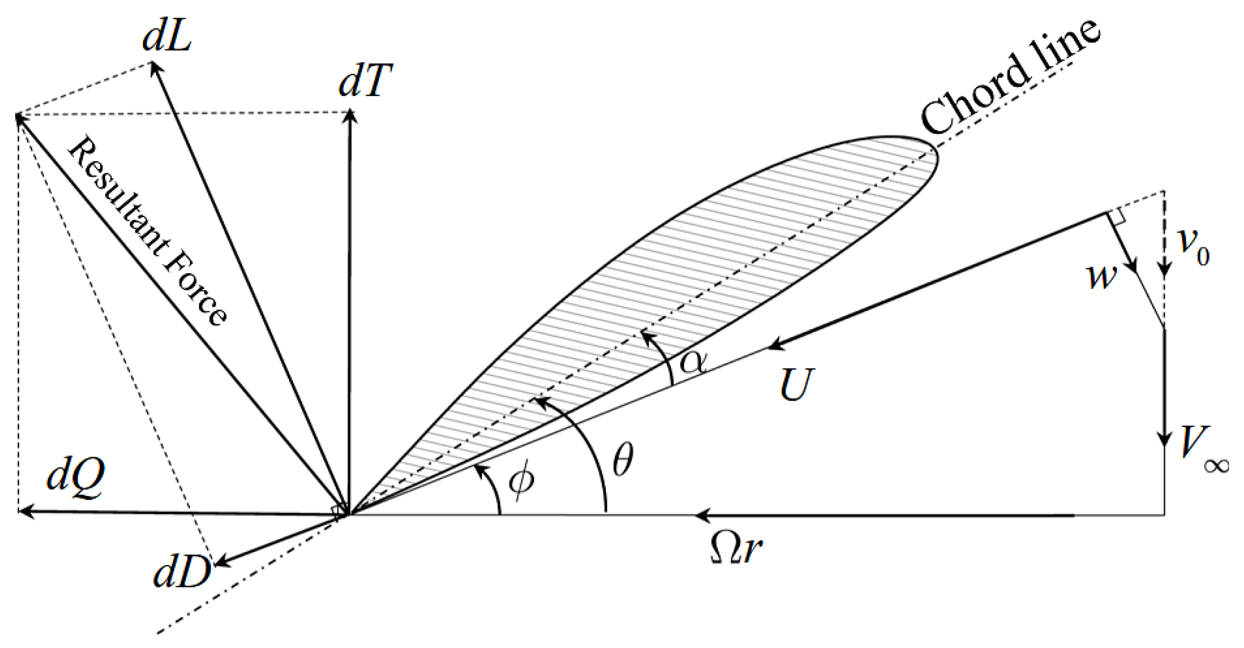
Initially, the proprotor’s operating conditions, including vortex wake displacement velocity ($v_0$), thrust coefficient ($C_T$), and power coefficient ($C_P$), are established. The vortex wake displacement velocity is assumed to remain constant in the radial direction, forming a rigid vortex sheet as the freestream passes through the proprotor disk. It is important to distinguish vortex wake displacement velocity ($v_0$) from wake convective velocity. While the latter includes contributions from both freestream and induced velocities, $v_0$ specifically refers to the velocity imparted by the rotational and translational motion of the proprotor blades.

The determination of ideal chord and twist distributions is grounded in the minimum energy loss theory, as introduced by Betz [42] and Glauert [43]. By minimizing energy loss at the design point, the bound circulation of the rotor blade element is given by the following equation:

$${\displaystyle \Gamma =\frac{4\pi R\overline{r}Fwsin\varphi }{N_b}=\frac{C_{l}cU}{2}}$$

(7)

where R is the blade radius, $\overline{r}=r/R$ is the non-dimensional radial station, F is the correction factor, w is the vortex-induced velocity, $\varphi$ is the inflow angle, $N_b$ is the number of blades, $C_l$ is the local lift coefficient, c is the local chord length, and U is the local flow velocity.

The local blade loading [44] is given by the following:

$$\left\{\begin{array}{c}\begin{array}{cc}\hfill {\displaystyle \frac{C_{l}c}{R}}& ={\displaystyle \frac{8\pi F\overline{r}\overline{w}sin\varphi }{N_b\overline{U}}}\hfill \\ \hfill {\displaystyle \overline{U}}& =\sqrt{{\mu }^2+{\overline{r}}^2-{\overline{w}}^2}={\displaystyle \frac{U}{\Omega R}}\hfill \end{array}\hfill \end{array}\right.$$

(8)

where $\mu =V_f/\Omega R$ is the advance ratio, $\overline{r}=\Omega r/\Omega R$ is the non-dimensional rotation velocity, and $\overline{w}=w/V_{tip}$ is the non-dimensional induced velocity, as shown in Figure 1. According to the principle of minimum energy loss [43,44], $w=v_{0}cos\varphi$, so w is perpendicular to U. $\overline{U}$ is the non-dimensional velocity, and F is the Prandtl tip loss factor, defined as follows:

$$F={\displaystyle \frac{2}{\pi }}{cos}^{-1}\left(exp\left({\displaystyle \frac{-N_b(1-\overline{r})}{2\overline{r}sin\varphi }}\right)\right)$$

(9)

By combining the above equations, the ideal chord distribution ${(c/R)}_{ideal}$ and twist distribution ${\theta }_{ideal}$ can be derived as ${(c/R)}_{ideal}={(C_{l}c/R)}_{ideal}/{C_l}_{ideal}$ and ${\theta }_{ideal}=\varphi +{\alpha }_{ideal}$, respectively. Here, ${C_l}_{ideal}$ denotes the local lift coefficient under ideal conditions, and ${\alpha }_{ideal}$ represents the angle of attack corresponding to the maximum lift-to-drag ratio.

The calculation of ideal chord and twist distributions is performed separately for hover and cruise conditions, with trim thrust and power coefficients used as constraints. An iterative calculation adjusts the vortex wake displacement velocity $v_0$ until the proprotor’s thrust coefficient ($C_T$) and power coefficient ($C_P$) match target values. The initial non-dimensional velocity is set to ${\overline{v}}_0=0.5\left(\sqrt{{\mu }^2+2{C_T}_0}-\mu \right)$, and is incrementally increased by $\delta =0.001$ until convergence is achieved.

The resulting ideal chord and twist distributions, calculated using the aforementioned methods, are then used to define the design bounds. To facilitate the initial design stage and ensure efficient optimization, positive and negative margins of 20% are applied to these ideal values. These adjusted bounds provide a suitable range for initializing the optimization process, allowing for rapid determination of design variables through low-fidelity models.

2.3. Rotor Wake rVPM Model

In the classical Vortex Particle Method (VPM) [45], the rotor wake is discretized into a vortex particle model with finite core sizes [46]. This method solves the vorticity form of the Navier–Stokes equations in a Lagrangian framework, with the governing equation expressed as follows:

$${\displaystyle \frac{D\overrightarrow{\omega }}{Dt}}=(\overrightarrow{\omega }·\nabla )\overrightarrow{u}+\nu {\nabla }^2\overrightarrow{\omega }$$

(10)

where $\overrightarrow{u}$ represents the flow velocity, $\nu$ is the kinematic viscosity of air, $\overrightarrow{\omega }=\nabla \times \overrightarrow{u}$ is the vorticity field, $D\left(\right)/Dt$ denotes the material derivative, and ${\nabla }^2$ is the Laplacian operator. The discretized vorticity field is given by the following:

$$\overrightarrow{\omega }(\overrightarrow{r},t)=\sum _{p=1}^{N_p}{\overrightarrow{\alpha }}_p\left(t\right){\zeta }_{{\sigma }_p}(\overrightarrow{r}-{\overrightarrow{r}}_p)$$

(11)

where $\overrightarrow{r}$ represents the spatial position, the subscript p denotes the p-th vortex particle, $N_p$ is the total number of vortex particles in the flow field, ${\overrightarrow{\alpha }}_p$ is the circulation strength of the p-th vortex particle, ${\zeta }_{{\sigma }_p}$ is the smoothing kernel function, and ${\sigma }_p$ is the core radius of the p-th particle. The smoothing kernel function is defined as follows:

$${\zeta }_{{\sigma }_p}\left(\overrightarrow{r}\right)={\displaystyle \frac{1}{{\sigma }_p^3}}\zeta \left({\displaystyle \frac{|\overrightarrow{r}|}{{\sigma }_p}}\right)$$

(12)

where $\zeta \left(\rho \right)={\left({\displaystyle \frac{2}{\pi }}\right)}^{1/2}exp\left(-{\displaystyle \frac{{\rho }^2}{2}}\right)$ is the Gaussian smoothing function.

The governing equations describing the evolution of vortex particle strength and spatial position are given by the following:

$$\left\{\begin{array}{c}\begin{array}{cc}\hfill {\displaystyle \frac{d{\overrightarrow{r}}_p}{dt}}& =\overrightarrow{u}({\overrightarrow{r}}_p,t),\hfill \\ \hfill {\displaystyle \frac{d{\overrightarrow{\alpha }}_p}{dt}}& =({\overrightarrow{\alpha }}_p·\nabla )\overrightarrow{u}({\overrightarrow{r}}_p,t)+\nu {\nabla }^2{\overrightarrow{\alpha }}_p.\hfill \end{array}\hfill \end{array}\right.$$

(13)

where the local velocity of the vortex particle $\overrightarrow{u}(\overrightarrow{r},t)={\overrightarrow{u}}_{\infty }(\overrightarrow{r},t)+{\overrightarrow{u}}_i(\overrightarrow{r},t)$ is composed of the freestream velocity ${\overrightarrow{u}}_{\infty }$ and the induced velocity ${\overrightarrow{u}}_i$ of the vorticity field. The induced velocity is obtained through the Biot–Savart law.

Although the classical Vortex Particle Method (VPM) achieves a balance between efficiency and accuracy in tiltrotor simulations [1,47], it frequently encounters numerical instability during the transition to turbulence, particularly in low-air-density environments [48]. These instabilities arise due to violations in the Lagrangian deformation and the incompressibility of the vorticity field [49].

To address these issues, this study adopts the reformulated Vortex Particle Method (rVPM) developed by Alvarez et al. [36,50]. The rVPM significantly enhances the conservation of local mass and angular momentum by dynamically adjusting particle sizes, improving numerical stability in simulations involving complex wake structures [36]. This reformulation refines the traditional vortex stretching and tilting mechanisms, ensuring enhanced conservation of mass and momentum, especially under high rotational speeds and complex blade–vortex interactions [51]. As a result, the prediction accuracy of aerodynamic loads and rotor performance metrics is significantly improved [52].

The key governing equations are adjusted to incorporate the evolution of vortex particle size, optimizing the method’s efficacy in simulating complex aerodynamic phenomena. These modifications are expressed as follows:

$$\left\{\begin{array}{ccc}{\displaystyle \frac{d}{dt}{\sigma }_p}\hfill & =& {\displaystyle -M_1\frac{{\sigma }_p}{\parallel {\overrightarrow{\alpha }}_p\parallel }\left[\left({\overrightarrow{\alpha }}_p·\nabla \right)\overrightarrow{u}\left({\overrightarrow{r}}_p\right)\right]·{\widehat{\alpha }}_p,}\hfill \\ {\displaystyle \frac{d}{dt}{\overrightarrow{\alpha }}_p}\hfill & =& {\displaystyle \left({\overrightarrow{\alpha }}_p·\nabla \right)\overrightarrow{u}\left({\overrightarrow{r}}_p\right)-M_2\left\{\left[\left({\overrightarrow{\alpha }}_p·\nabla \right)\overrightarrow{u}\left({\overrightarrow{r}}_p\right)\right]·{\widehat{\alpha }}_p\right\}{\widehat{\alpha }}_p,}\hfill \\ {\displaystyle \frac{d}{dt}\overrightarrow{\omega }{|}_{\mathrm{viscous}}}\hfill & =& {\displaystyle \nu {\nabla }^2\overrightarrow{\omega }.}\hfill \end{array}\right.$$

(14)

In these equations, ${\sigma }_p\left(t\right)=\sigma ({\overrightarrow{r}}_p,t)$ is the filter width at the position of the p-th particle, $d{\sigma }_p/dt$ governs the evolution of the vortex particle size, and ${\widehat{\alpha }}_p$ represents the filtered vorticity strength. The coefficients $M_1$ and $M_2$, as defined in Equation (15), ensure the conservation of angular momentum and mass within the vortex core.

$$\left\{\begin{array}{c}\begin{array}{cc}\hfill M_1& ={\displaystyle \frac{g+f}{1+3f}},\hfill \\ \hfill M_2& ={\displaystyle \frac{g+f}{1/3+f}}.\hfill \end{array}\hfill \end{array}\right.$$

(15)

Additionally, the Particle Strength Exchange (PSE) method [53] is employed to handle viscous diffusion, allowing for accurate resolution of the diffusion term in the governing equations. The PSE method ensures that the diffusion of vorticity is accurately captured without introducing significant numerical diffusion, a common issue in traditional vortex methods.

To further enhance computational efficiency, the Fast Multipole Method (FMM) [54] is incorporated to accelerate the N-body problem associated with calculating the induced velocity of each vortex particle. The FMM reduces the computational complexity from $O\left(N^2\right)$ to approximately $O\left(N\right)$, enabling the simulation of large-scale vortex systems with significantly improved performance.

Moreover, to improve the stability and accuracy of the rVPM, Large Eddy Simulation (LES) principles are incorporated into the framework. LES models the effects of smaller, unresolved scales by introducing a subgrid-scale stress tensor, $T_{ij}\equiv \overline{u_i{\omega }_j}-\overline{u_i}\overline{{\omega }_j}$ [36]. This tensor captures the interactions between the resolved large-scale dynamics and the unresolved subgrid-scale dynamics, which are crucial for accurately modeling turbulence. The LES-filtered Navier–Stokes equations, expressed in vorticity form, are given by the following:

$${\displaystyle \frac{d}{dt}}\overrightarrow{\omega }=(\overrightarrow{\omega }·\nabla )\overrightarrow{u}+\nu {\nabla }^2\overrightarrow{\omega }-E_{adv}-E_{str}$$

(16)

where ${\left(E_{adv}\right)}_i\equiv \partial T_{ij}^{\prime }/\partial x_j$ represents the subfilter-scale (SFS) vorticity advection, and ${\left(E_{str}\right)}_i\equiv -\partial T_{ij}/\partial x_j$ represents SFS vortex stretching.

By integrating LES principles into the rVPM, this study introduces a numerically stable and grid-free LES scheme which not only preserves vortex structures but also eliminates the need for complex grid generation, avoiding the numerical dissipation typically associated with grid-based CFD methods. The scheme is further enhanced by not being constrained by the Courant–Friedrichs–Lewy (CFL) condition, allowing for larger time steps and faster simulations. For a comprehensive mathematical derivation of this method, please refer to [36].

In summary, the rVPM, with its enhanced particle size evolution mechanism and incorporation of LES principles, significantly improves the stability and computational efficiency of Vortex Particle Methods, making it highly applicable for rotor performance evaluation in various aerodynamic environments. This method offers a robust and efficient tool for accurately predicting the aerodynamic characteristics of proprotors in both hover and high-altitude cruise.

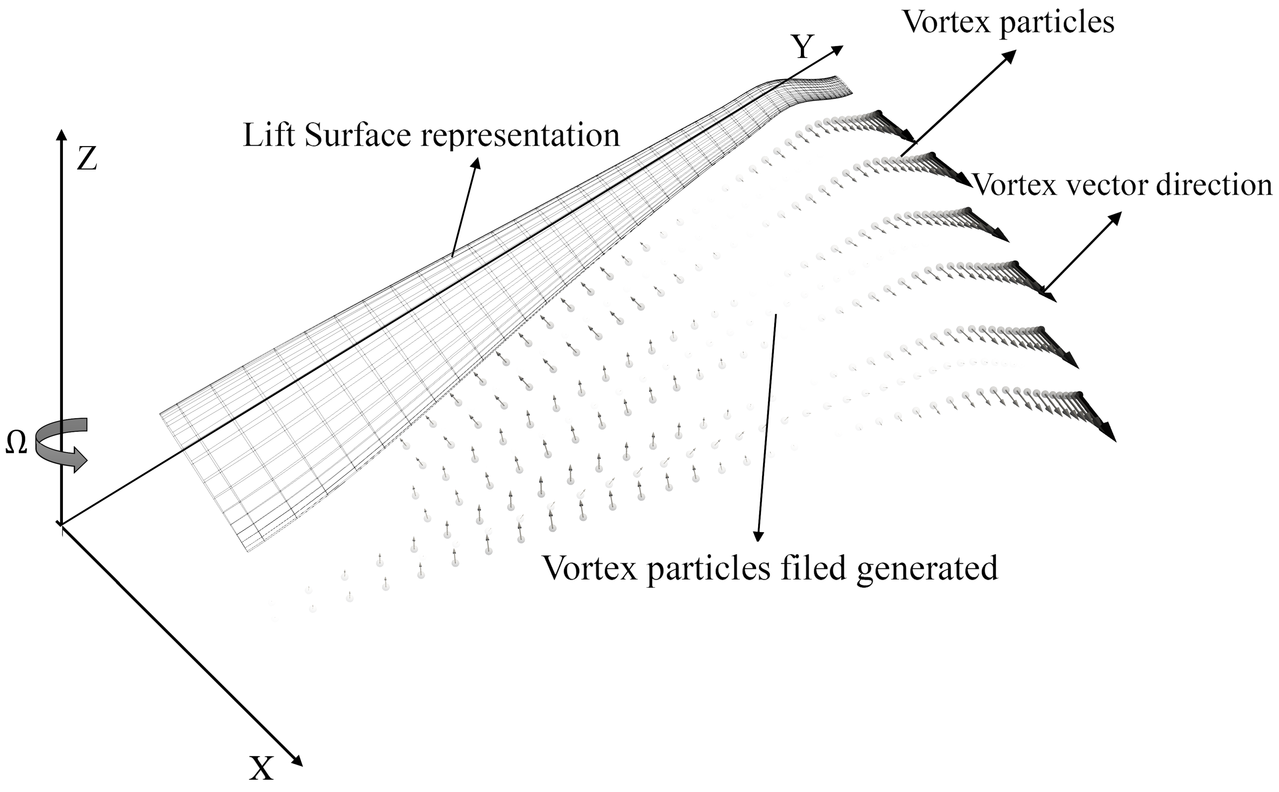
2.4. Rotor Blade Lifting Surface Model

The aerodynamic model of proprotor blades requires accurate computation of rotor thrust and induced velocity. Traditionally, the Lifting-Line Method (LLM) and Lifting Surface Method (LSM) have been widely used, often in conjunction with the Vortex Particle Method [55]. The Lifting Surface Method provides higher computational accuracy, especially for analyzing three-dimensional blade shapes with a taper and anhedral. Thus, the Lifting Surface Method is employed in this study to model the rotor blades’ aerodynamics.

In this approach, the blade is discretized into infinitesimal segments along the span, represented by a mean camber surface with zero thickness. For blades with sweep and taper, the grid lines at the leading and trailing edges are adjusted accordingly. Each blade segment is divided into columns along the span and rows along the chord, forming a grid system. Spanwise bound vortices are positioned at the quarter-chord line, while chordwise bound vortices are arranged along the spanwise grid. The trailing edge vortex is located at the quarter-chord line of the adjacent grid, and the vortex grid at the trailing edge generates vortex particles that shed into the rotor wake.

The vortex sources generated at the trailing edge are calculated using the following formula:

$${\overrightarrow{\gamma }}_{\mathrm{wake}}=-{\displaystyle \frac{d{\overrightarrow{\Gamma }}_b}{dt}}+{\overrightarrow{v}}_b\nabla ·{\overrightarrow{\Gamma }}_b$$

(17)

where ${\overrightarrow{\gamma }}_{\mathrm{wake}}$ is the strength of the newly generated vortex, ${\overrightarrow{\Gamma }}_b$ represents the bound circulation of the blade, and ${\overrightarrow{v}}_b$ is the local velocity of the bound vortex, including contributions from blade rotation, freestream, induced velocity, and interference. The first term accounts for the trailing vortex generated by spanwise variation in bound circulation, while the second term represents the shedding vortex due to azimuthal variations. To ensure stability, the Kutta condition is applied at the trailing edge at each time step, maintaining vorticity balance.

The total circulation source $\overrightarrow{\gamma }$, generated from changes in bound circulation, is distributed across an interpolation surface representing the blade’s convective trajectory. The vortex particle field is initialized based on this circulation source, allowing for accurate coupling between the vortex particle field and the lifting surface. This coupling forms the rVPM/LSM aerodynamic analysis model, as illustrated in Figure 2.

After determining the bound circulation, aerodynamic forces on the blade sections are calculated using the Kutta–Joukowski theorem. To account for viscous effects, corrections are applied using pre-generated airfoil C81 data tables, allowing for a more accurate estimation of profile drag. For implementation details, including code, please refer to the open-source rotor aerodynamic analysis package DUST, provided by Montagnani et al. on GitLab [56].

2.5. Model Validation

To assess the accuracy of the developed rVPM/LSM model in calculating the aerodynamic characteristics of proprotors, several rotor and propeller models were simulated and compared against experimental data and CFD results. In all validation cases, a consistent set of simulation settings was applied. The minimum time step was set to $\pi /90$ radians, and the wake was truncated when it extended beyond a cube with a side length of $10R$ centered at the rotor hub. The initial vortex particle size was set to 1.2 times the local lifting surface grid size, ensuring overlap between particles. The blade lifting surface was divided into 50 radial sections and 5 chordwise sections, with additional refinement near the blade tip.

Each simulation ran for at least 12 revolutions, and convergence was confirmed if either the average wake position changed by less than 2.5% or the average thrust varied by less than 1% over two consecutive revolutions. Once convergence was achieved, the time-averaged results from the final revolution were used.

Initially, a parametric model was constructed based on the proprotor designed by Droandi et al. [24], and the results were compared with hover test and CFD results. The results are shown in Figure 3.

As is evident from the figure, the computational results of the rVPM/LSM model demonstrate good agreement with both the experimental data and CFD results. This indicates that the rVPM/LSM model employed in this study exhibits high accuracy and reliability in predicting the hover performance of proprotors, achieving a level of confidence comparable to CFD.

Subsequently, a computational model of the Beaver propeller was established, drawing upon experimental data from Dr. Veldhuis’s dissertation [57]. The results were then compared with experimental data [58] and computational results based on the rVPM and actuator line model by Alvarez [51]. These comparisons are presented in Figure 4. Figure 4a illustrates the evolution of the Beaver propeller wake flow field after five revolutions under conditions of an advance ratio $J=0.8$ and freestream velocity $V_f=40\mathrm{m}/\mathrm{s}$. Figure 4b depicts the variation of the thrust coefficient ($C_T$) with the advance ratio (J), while Figure 4c shows the variation of cruise efficiency ($\eta$) with the advance ratio (J). The figures reveal that the present model’s predictions of thrust coefficient and cruise efficiency align well with experimental data across the entire range of advance ratios. Discrepancies between the present model and Alvarez’s model may be attributed to the fact that the actuator line model relies on the C81 airfoil data table, whereas the present model employs the Lifting Surface Method.

Additionally, the BEMT method based on Xfoil airfoil data [22] is included in the figure. As shown, the BEMT method aligns well with experimental data in terms of thrust coefficient prediction, with minor deviations at lower advance ratios, likely due to low Reynolds number effects. For cruise efficiency, the BEMT method also exhibits satisfactory agreement, with a slight overestimation at moderate advance ratios. This comparison demonstrates that the BEMT method can achieve rapid iteration while maintaining sufficient accuracy in predicting proprotor performance. Our method, while significantly less efficient in rapid iteration compared to the BEMT method, performs better than CFD methods. Additionally, it offers advantages in analyzing blades with nonlinear planforms and tip anhedral designs, showcasing its potential for further development. Therefore, our method essentially represents a compromise between BEMT and CFD methods, balancing computational efficiency with the ability to cover a broader range of design variables. Overall, the present model’s calculations of cruise efficiency for proprotors exhibit consistency with both experimental data and validated computational results, affirming its effectiveness.

Finally, a model of the classic XV-15 three-blade tiltrotor was constructed and simulated. Geometric parameters of the blades (including planform shape, chord distribution, and twist distribution) were sourced from the literature [59], and comparisons were made with wind tunnel test data for the XV-15 in hover and forward flight at a tip Mach number of 0.66 [60], as well as CFD results [30]. The results are presented in Figure 5 and Figure 6.

Figure 5 illustrates the wake field of the XV-15 rotor in (a) hover with a tip Mach number of $M_{tip}=0.66$ and (c) a typical cruise condition at $V_f=0.7\Omega R$. Figure 5b shows the different collective pitch of the proprotor in different operational conditions. Figure 6a shows the variation of the figure of merit ($FM$) with the rotor blade loading coefficient ($C_T/\sigma$), while Figure 6b depicts the variation of cruise efficiency (${\eta }_{cruise}$) with the rotor blade loading coefficient ($C_T/\sigma$).

The figures reveal that the present model demonstrates good agreement with experimental data for both hover and forward flight conditions of the XV-15 tiltrotor. Discrepancies between the model’s results and the CFD results may be attributed to the differences in the airfoil modeling between the two methods.

Table 1. Model error analysis.

Metric	Droandi ($\mathbf{FM}$)	Droandi (${\mathit{C}}_{\mathit{P}}$)	Beaver (${\mathit{C}}_{\mathit{T}}$)	Beaver ($\mathit{\eta }$)	XV-15 ($\mathbf{FM}$)	XV-15 ($\mathit{\eta }$)
RMSE	0.0217	0.0004	0.0097	0.0418	0.0220	0.0428
MAE	0.0124	0.0004	0.0057	0.0375	0.0171	0.0291
MAPE	5.15%	8.07%	8.65%	9.57%	2.59%	4.81%

summarizes the root mean squared error (RMSE), mean absolute error (MAE), and mean absolute percentage error (MAPE) between the rVPM/LSM model and the experimental data for the three computational cases discussed in this section. Generally, an RMSE within 0.01 and an MAPE within 5% are considered to indicate high fidelity; an RMSE between 0.01 and 0.05 and an MAPE between 5 and 10% signify medium fidelity; and exceeding these ranges indicates low fidelity. The results in Table 1 demonstrate that the RMSE between the rVPM/LSM model and the experimental data ranges from 0.0004 to 0.0428, and the MAPE ranges from 2.59% to 9.57%.

Therefore, it can be concluded that the rVPM/LSM model developed in this study achieves medium-to-high fidelity in estimating tiltrotor performance, rendering it suitable for multi-objective optimization tasks in the preliminary design phase of proprotors.

On the workstation configuration detailed in

Table 2. Workstation specifications employed in this study.

Component	Specification
Processor	AMD Ryzen Threadripper 3990X 64-Core Processor 2.90 GHz
Memory	128 GB (128 GB available)
System Type	64-Bit Operating System, x64-Based Processor

, the developed rVPM/LSM coupled model achieves single-point computation times ranging from 2.5 to 4.5 min, while single control input trim computation times range from 6 to 15 min. Notably, the trim time can be further reduced by utilizing gradient data precomputed based on the BEMT method.

In contrast, conventional grid-based CFD methods employing the Reynolds-Averaged Navier–Stokes (RANS) equation [30] exhibit single-point computation times of 20 to 60 min, and the lattice Boltzmann methods (LBM) [61] require at least 40 min, with neither accounting for control input trimming. Thus, the developed model strikes a favorable balance between accuracy and computational iteration cycle time, rendering it well suited for multi-objective design optimization tasks for proprotor blade aerodynamic shapes.

While CFD and LBM offer distinct advantages in capturing detailed flow features or vortex–surface interactions, the present method excels in balancing efficiency and accuracy for the preliminary design stage, where rapid iteration is paramount.

3. Design Optimization Framework

Figure 7 illustrates the comprehensive design optimization framework employed in this study. The framework encompasses three distinct stages.

• Rapid Estimation of Overall Parameters: Based on the mission requirements, a rapid estimation model is utilized to determine the overall parameters of the proprotor, encompassing rotor diameter, solidity, and rotational speed. These determined parameters are then passed to the subsequent stage.
• Estimation of Ideal Chord and Twist Distributions: The overall parameters obtained from the first stage are input into the ideal chord and twist distribution estimation model. Through this model, the optimal values for chord and twist distributions under hover and cruise conditions are determined based on the rigid vortex wake model and the principle of minimum energy loss. A positive and negative margin of 20% is then applied to establish the upper and lower bounds. The smallest value among these is taken as the lower boundary, and the largest value is taken as the upper boundary for the design variables. Subsequently, the range for the blade tip anhedral angle and its starting position is also specified. Finally, the radial distribution of the airfoil is determined according to the aerodynamic characteristics of typical flight conditions.
• Optimization Search Process: During the optimization search process, a many-objective hybrid optimizer (MOHO) is employed. The MOHO combines various optimization algorithms such as the NSGA-III, MOEA-DD, SPEA-R, NSDE-R1B, and NSDE-D3, dynamically selecting the most suitable optimization strategy based on the performance of each algorithm at the current stage. The initial population is randomly generated within the defined design bounds for chord and twist distributions, and the objective function values are calculated using the reformulated Vortex Particle Method (rVPM) and Lifting Surface Model (LSM). The MOHO enhances search efficiency and effectiveness through its dynamic switching mechanism. Each iteration includes at least 66 individuals, with a total of 50 search generations, ultimately yielding optimized blade designs.

This optimization framework ensures a systematic and rigorous design process, enhancing design efficiency while maintaining computational accuracy.

3.1. Design Requirements and Determination of Overall Parameters

The objective of this research is to optimize the aerodynamic design of proprotor blades to meet the dual requirements of efficient low-altitude hover and high-altitude cruise flight. The specific design requirements are outlined in

Table 3. Key design parameter ranges and performance index requirements.

Design Parameter	Value Range/Requirement
Number of Blades	3
Rotor Diameter	2.5–3.3 m
Tip Speed	160–220 m/s
Solidity	0.07–0.12
Hover Thrust	2000 N
Hover Efficiency	≥0.70 ($\rho$ = 1.225 kg/m3)
Maximum Thrust	2600 N
Forward Flight Thrust	350 N
Forward Flight Speed	80 m/s
Propulsive Efficiency	≥0.75 (4500 m Altitude, $\rho$ = 0.78 kg/m3)
Hover Speed	1200–1350 RPM
Forward Flight Speed	70% of Hover Speed

. Based on these mission requirements, the number of rotor blades is fixed at 3, the rotor diameter is constrained between 2.5 m and 3.3 m, and the rotor hover speed ranges from 1200 to 1350 RPM, with a solidity requirement between 0.07 and 0.12.

In terms of hover performance, the rotor is mandated to provide a hover thrust of 2000 N with a hover efficiency of no less than 0.70, evaluated at a standard atmospheric density of 1.225 kg/m³. To accommodate high thrust demands and ensure design robustness, the maximum thrust of the rotor in this state must not be less than 2600 N.

For forward flight performance, the propulsive efficiency should not fall below 0.75 at an altitude of 4500 m, a cruise speed of 80 m/s, and a design forward flight thrust of 350 N. The atmospheric density for this operating condition is derived from the International Standard Atmosphere table and is calculated as 0.78 kg/m³. Additionally, the forward flight speed should be approximately 70% of the hover speed. To address the high thrust requirements and maintain design robustness, the maximum thrust of the rotor in this state must not be less than 525 N.

After establishing the design objectives, these parameters are input into the rapid estimation model for the overall parameters to generate a set of feasible solutions, which are then weighted and ranked. Considering that the primary operating state of the proprotor is high-altitude cruise, the hover efficiency weight is set to 40%, and the high-altitude cruise propulsive efficiency weight is set to 60%. Based on the ranking results, the key design parameters of the proprotor with the optimal figure of merit are presented in

Table 4. Key overall design parameters of the tiltrotor.

Design Parameter	Value
Number of Blades	3
Rotor Diameter	2.7 m
Solidity	0.08 ± 0.005
Rotation Speed	Hover: 1200 RPM
	Forward Flight: 900 RPM

.

3.2. Determination of Blade Shape Design Variables and Bounds

The chord and twist distributions of the proprotor blades are parameterized using B-spline curves. A B-spline curve is a linear combination of a set of B-spline basis functions where the $n_{th}$ order corresponds to a spline curve of degree $m=n-1$. A B-spline curve can be expressed as follows:

$$\mathbf{x}\left(t\right)=\sum _{i=0}^{N+n}{\beta }_i{\mathbf{N}}_{i,n}\left(t\right)\mathrm{for}t\in [t_0,t_{N+n}]$$

(18)

where ${\beta }_i$ are the control points, N is the number of internal knots of the B-spline curve, ${\mathbf{N}}_{i,n}\left(t\right)$ are the basis functions, $\mathbf{x}$ represents the sample point position, and $[t_0,t_{N+n}]$ represents the domain of the sample points. The geometric shape can be determined by $K=N+n+1$ control points. In this study, the chord length and twist distribution curves of the high-altitude proprotor blades are represented by B-spline curves with five and four control points, respectively.

Previous studies have indicated that quadratic or cubic S-splines are generally sufficient for representing chord and twist distributions. However, in this work, five and four control points were chosen empirically to provide sufficient flexibility in capturing the geometric variations in blade chord length and twist. The spline curve equations are as follows:

$$Ch\left(r\right)=\sum _{i=0}^4{c}_i{\mathbf{B}}_{i,3}\left(r\right)\mathrm{for}r\in [0,1]$$

(19)

$$\theta \left(r\right)=\sum _{i=0}^3{t}_i{\mathbf{B}}_{i,2}\left(r\right)\mathrm{for}r\in [0,1]$$

(20)

where $Ch$ represents the chord length, $\theta$ represents the twist angle, $c_i$ are the control point parameters for the chord length distribution B-spline curve, and $t_i$ are the control point parameters for the twist distribution B-spline curve. The number of control points was determined empirically, with five and four found to be sufficient to represent the variations in blade chord length and twist, respectively. While limiting the number of control points can constrain the shape to more conventional geometries, using a higher number of control points provides the potential for generating more unique or exotic shapes, which may offer advantages in exploring unconventional designs. The B-spline curve for chord length distribution is represented by $[c_1,c_2,c_3,c_4,c_5]$ as control point parameters, and the twist distribution spline is represented similarly. Through linear combinations of different basis functions and control point parameters, any curve shape within the range of $[0.0,1.0]$ can be generated.

In addition to chord and twist, recognizing that blade tip anhedral can enhance both hover efficiency and potentially cruise efficiency [20]. The starting radial position and angle of the anhedral are also incorporated as design variables in this study. Therefore, the rotor blade is characterized by a total of 11 design variables, forming a vector $\mathbf{X}$ defined as follows:

$$\mathbf{X}=[c_1,c_2,c_3,c_4,c_5,t_1,t_2,t_3,t_4,r_{ahd},{\alpha }_{ahd}]$$

(21)

where $r_{ahd}$ denotes the non-dimensional radial position of the blade tip anhedral start point, and ${\alpha }_{ahd}$ denotes the blade tip anhedral angle (negative values indicate wash-in). The design variable bounds are established based on the estimated model for optimal chord and twist distribution, while the radial position and angle of the anhedral are determined based on practical engineering and manufacturing constraints. The range of each variable is summarized in

Table 5. Design variable ranges.

Variable	${\mathit{c}}_1$	${\mathit{c}}_2$	${\mathit{c}}_3$	${\mathit{c}}_4$	${\mathit{c}}_5$	${\mathit{t}}_1$	${\mathit{t}}_2$	${\mathit{t}}_3$	${\mathit{t}}_4$	${\mathit{r}}_{\mathit{ahd}}$	${\mathit{\alpha }}_{\mathit{ahd}}$
Upper Limit	0.20	0.30	0.25	0.20	0.10	30.0	15.0	5.0	1.0	0.95	30.0°
Lower Limit	0.05	0.03	0.01	0.01	0.01	8.0	−5.0	−15.0	−15.0	0.88	−10.0°

.

Figure 8 illustrates the blade planform shape fitted with B-splines (a), the variation of the blade installation angle and the effect of blade tip anhedral (b), the chord length distribution curve fitted with B-splines (c), and the twist distribution curve fitted with B-splines (d). Overall, the B-spline fitting scheme adopted in this study effectively represents blade shapes with nonlinear chord length, twist distribution, and blade tip anhedral design.

The selection and arrangement of blade airfoils are primarily determined based on the Reynolds number (Re), Mach number (Ma), and ideal angle of attack distribution at different radial stations under representative operating conditions. Figure 9 illustrates the distribution of Reynolds and Mach numbers at various radial stations of the blade in typical hover and cruise conditions. Both Ma and Re increase with the radius, exhibiting more pronounced variations in hover. In both flight conditions, the maximum Ma remains below 0.5, indicating negligible compressibility effects. The Re in cruise conditions varies between $0.5\times {10}^6$ and $1\times {10}^6$ across the entire radius. While in hover, it ranges from $0.5\times {10}^6$ to $2\times {10}^6$.

Figure 10 compares the lift-to-drag ratio of selected airfoils under Re and Ma conditions corresponding to the root and 0.7R stations in typical hover and cruise conditions. The OA212 airfoil demonstrates a superior lift-to-drag ratio at low Re and low Ma with angles of attack exceeding $8^{\circ }$, making it suitable for the inner blade section. The NACA4412 airfoil performs well in both conditions near a $0^{\circ }$ angle of attack, rendering it suitable for the outer section. The Boeing106 and VR07 airfoils exhibit excellent lift-to-drag ratio performance at moderate-to-small angles of attack, making them suitable for the middle section. The final radial distribution of airfoils is determined by calculating the lift and drag characteristics of each radial station airfoil based on the optimal chord and twist distributions, ensuring smooth and continuous airfoil transitions.

Table 6. Radial distribution of airfoils.

r/R	0.15–0.35	0.35–0.75	0.75–0.90	0.90–1.00
Airfoil	OA212	Boeing106	VR07	NACA4412

presents the pre-arranged radial distribution of airfoils. This pre-arrangement significantly reduces the number of design variables, thereby enhancing computational efficiency during the optimization search process. Notably, the optimization framework in this study is fully capable of incorporating airfoil selection and distribution as design variables into the optimization search process. The inclusion of more selectable airfoils and parameterized airfoil profiles will be explored in future research.

3.3. Optimization Objectives and Constraints

In this study, the primary optimization objectives for the proprotor system were to maximize both the figure of merit ($FM$) in hover and the propulsive efficiency ($\eta$) in high-altitude cruise. These objectives are paramount for enhancing the overall aerodynamic efficiency and performance of the tiltrotor across its operational envelope.

The figure of merit, a key performance indicator in rotorcraft aerodynamics, is often defined as the ratio of ideal power to actual power required for hovering. It quantifies the efficiency of the tiltrotor during hover, and optimizing this metric directly translates to improved hover performance and reduced power consumption during hover, which is essential for vertical take-off and landing (VTOL) aircraft. Similarly, the propulsive efficiency during high-altitude cruise is critical for improving the cruise efficiency of unmanned tiltrotors. This parameter directly impacts the aircraft’s fuel consumption and, consequently, its range. Optimizing the rotor blade geometry to enhance propulsive efficiency under cruise conditions ensures superior performance throughout the aircraft’s flight envelope.

Therefore, the optimization objective of this study was formulated as the maximization of both the figure of merit and the propulsive efficiency in high-altitude cruise, subject to fundamental design constraints.

$$\begin{array}{cc}\hfill \mathrm{Find}\text{:}& \mathbf{x}=[c_1,c_2,c_3,c_4,c_5,t_1,t_2,t_3,t_4,r_{ahd},{\alpha }_{ahd}]\hfill \\ \hfill \mathrm{Max}\text{:}& FM\left(\mathbf{x}\right)={\displaystyle \frac{C_T^{3/2}}{\sqrt{2}{C}_P}};\eta \left(\mathbf{x}\right)={\displaystyle \frac{T{V}_{\infty }}{P}}={\displaystyle \frac{\mu C_T}{C_P}}\hfill \\ \hfill \mathrm{S}.\mathrm{T}.\text{:}& \left(1\right)|T-T\left(\mathbf{x}\right)|\le 0.25\%\times T(T_{hover}=2000\mathrm{N},T_{cruise}=350\mathrm{N})\hfill \\ \hfill & \left(2\right)P\left(\mathbf{x}\right)\le 35\mathrm{kW}\hfill \\ \hfill & \left(3\right)0.06\le \sigma \le 0.115\hfill \end{array}$$

(22)

To ensure the practicality and feasibility of the design results, a series of constraints was imposed, encompassing maximum rotor thrust, power limits, objective bounds, rotor solidity limits, and blade planform shape constraints. The specific constraints are detailed in

Table 7. Design constraints.

Constraint Variable	Constraint Condition
Maximum Thrust	$T_{max}\ge 1.3\times T_{hover}$ (hover condition)
Power Limit	$P\le 35\mathrm{kW}$ (both hover and cruise)
Objective Boundary	$FM\ge 0.70;\eta \ge 0.75$
Rotor Solidity	$0.06\le \sigma \le 0.115$
Planform Shape	$c^{″}\left(r\right)\ge 0$

. Notably, the rotor solidity bounds were determined based on a sensitivity analysis of the rapid estimation model for the overall parameters and the upper and lower limits of the ideal chord length. The planform shape constraints primarily serve to prevent the spline curve parameters from generating unrealistic or singular shapes.

3.4. Optimization Strategy

The aerodynamic shape design of proprotor blades presents a multi-objective optimization problem characterized by numerous design variables, lengthy iteration cycles, and a non-convex solution space. Consequently, the optimization strategy must balance efficiency and global search capability, often conflicting objectives. Classic global algorithms, such as genetic algorithms, necessitate repeated calls to the rVPM/LSM method to evaluate objective functions for a large population of individuals, resulting in low optimization efficiency. Conversely, conventional nonlinear programming algorithms are prone to converging to local optima, potentially missing the global optimum.

To address these challenges, this study employs a many-objective hybrid optimizer (MOHO) [62] as the optimization strategy for proprotor blade aerodynamic shape design. The MOHO is a versatile algorithm designed to tackle multi-objective optimization problems, particularly well suited for scenarios with complex design variables and computationally intensive evaluations. By integrating multiple optimization algorithms and dynamically switching among them based on their real-time performance, the MOHO overcomes the limitations of single algorithms in complex optimization landscapes.

Evolutionary algorithms (EAs) were selected for their ability to handle high-dimensional, multi-objective, and nonlinear optimization problems with complex design variables. EAs have been shown to be effective in exploring large and complex search spaces without relying on gradient information, which is often unavailable or unreliable in aerodynamic shape optimization tasks. Additionally, EAs can efficiently manage nonlinear constraints and discontinuities, which are common in multi-objective aerodynamic design.

The MOHO framework incorporates five distinct base optimization algorithms, each with unique strengths in handling specific types of optimization problems:

• NSGA-III (Non-Dominated Sorting Genetic Algorithm III) [63]: A genetic algorithm tailored for multi-objective optimization employing simulated binary crossover (SBX) and polynomial mutation operators to effectively navigate the multi-objective landscape.
• MOEA-DD (Many-Objective Evolutionary Algorithm Based on Dominance and Decomposition) [64]: A multi-objective evolutionary algorithm leveraging dominance and decomposition principles utilizing penalty boundary intersection (PBI) metrics for selection to ensure diversity and convergence of solutions.
• SPEA-R (Strength Pareto Evolutionary Algorithm Based on Reference Point) [65]: A strength Pareto evolutionary algorithm employing reference points to prioritize solution diversity and maintain a uniform distribution of the Pareto front.
• NSDE-R1B (Non-Dominated Sorting Differential Evolution with Rand/1/Bin Mutation) [66]: A differential evolution algorithm utilizing rand/1/bin mutation operators to facilitate rapid exploration of the design space.
• NSDE-D3 (Non-Dominated Sorting Differential Evolution with Donor3 Mutation): A differential evolution algorithm employing the donor3 mutation operator, enhancing search efficiency through weighted combinations of parent designs.

The core advantage of the MOHO lies in its dynamic switching mechanism. By monitoring the performance of each algorithm in each generation and switching based on the probability of success (POS) values, the MOHO adaptively selects the most suitable optimization strategy. The POS value reflects the effectiveness of each algorithm in the current optimization stage and is calculated as follows:

$$POS(·)={\displaystyle \frac{N_{success}(·)}{N_{total}(·)}}$$

(23)

where $N_{success}(·)$ is the number of successful attempts, and $N_{total}(·)$ is the total number of attempts. By dynamically selecting the algorithm with the highest POS value, the MOHO can leverage the most appropriate algorithm at different stages of the optimization process, thereby enhancing overall optimization efficiency and effectiveness.

The MOHO demonstrates significant advantages in maintaining solution diversity and accelerating convergence. Its reference point partitioning technique ensures uniform exploration of the solution space, mitigating the risk of converging to local optima. Simultaneously, by integrating the strengths of different algorithms, the MOHO can more rapidly approach the global optimum, significantly accelerating convergence.

Employing the MOHO as the optimization strategy for proprotor blade aerodynamic shape design effectively improves optimization efficiency while ensuring global search capability, maintaining solution diversity, and facilitating convergence. This versatile optimization strategy is not only applicable to the current research problem but also holds broad potential for future rotorcraft aerodynamic design optimization, providing a robust theoretical and practical foundation.

4. Results and Discussion

4.1. Optimization Process and Results

Following the strategy outlined in the preceding section, the bounds of the blade design variables were initially determined based on the estimated model for ideal chord and twist distributions. Within these boundary ranges, 66 distinct design parameter sets were randomly generated as the initial population. The objective function values for all individuals within this initial population were computed using the rVPM/LSM model. Subsequently, the design parameters and objective function values of these initial populations were passed to the MOHO optimization strategy for iterative searching to identify the global optimal solution.

Based on this search methodology, three distinct optimization objectives were pursued: optimizing for $FM$, optimizing for $\eta$, and optimizing for a weighted combination of $(0.4FM+0.6\eta )$. The chosen weighting of 40% $FM$ and 60% $\eta$ was based on the dual requirements of optimizing the proprotor’s performance during both hover and cruise phases. Maximizing $FM$ is crucial for ensuring effective vertical take-off and landing capabilities with lower power consumption, while cruise efficiency ($\eta$) is essential for minimizing fuel consumption and maximizing range during forward flight. Given the primary mission profile of this tiltrotor, which involves extended cruise phases interspersed with occasional hover operations, the chosen weighting aims to strike a balance between these competing objectives.

Each optimization objective was iteratively advanced for 50 generations, with each generation comprising 66 individuals. Figure 11 illustrates the search processes for the three optimization objectives. Each dot in the figures represents the best individual of the current generation, while the bar chart depicts the relative percentage change in the objective function value of the best individual in each generation. Convergence is deemed to have been achieved when the relative percentage change remains below 0.25% for 10 consecutive generations.

As shown in Figure 11a, the change in hover $FM$ is relatively rapid in the initial 10 generations, slowing down between the 10th and 20th generations, and further decreasing between the 20th and 30th generations. From the 30th generation onwards, the value of the best individual in each generation stabilizes, with the magnitude of change remaining within 0.001. The relative percentage change in $FM$ remains below 0.25% for 10 consecutive generations, indicating convergence of the hover objective search.

Figure 11b reveals that, when optimizing for $\eta$, the changes are more substantial in the first 10 generations, potentially due to a larger optimization space for $\eta$ in typical cruise conditions. Despite the significant changes in the initial 10 generations, the trend rapidly diminishes from the 10th to the 20th generation. Beyond the 20th generation, the optimal cruise efficiency increases gradually and stabilizes. From the 40th to the 50th generation, the magnitude of the change in $\eta$ remains within 0.001, and the relative percentage change stays below 0.25% for 10 consecutive generations, signifying convergence of the cruise objective search.

Figure 11c illustrates that the optimization hierarchy for the weighted objective is more pronounced. After an initial jump from the first to the second generation, the value gradually rises, followed by a smaller jump within 10 generations. Subsequently, it rises again slowly, with another minor jump occurring within the 20th generation. From the 20th to the 40th generation, the weighted objective value increases steadily. From the 40th to the 50th generation, the weighted objective value stabilizes, with the magnitude of change remaining within 0.001 and the relative percentage change staying below 0.25% for 10 consecutive generations, indicating convergence of the weighted objective search.

4.2. Pareto Front Analysis

Upon obtaining the results of the three distinct search paths targeting pure hover objectives, pure cruise objectives, and weighted objectives, and eliminating individuals that violated constraints or exhibited excessive distortion or extreme twist, all feasible solutions were aggregated to form a Pareto front scatter plot, as depicted in Figure 12. This figure reveals that, as iterations progress, the overall population evolves towards the upper-right region of the initial population, indicating higher hover figure of merit ($FM$) and cruise efficiency ($\eta$), despite some individual points potentially performing worse than the initial population. Clusters of populations suggest potential local optima encountered during the search process. As iterations continue, a series of feasible solutions exhibiting excellent performance in both $FM$ and $\eta$ are ultimately obtained, forming the Pareto front curve. The individual with the highest $FM$ value is designated as the “opt_hover” configuration, the individual with the highest $\eta$ value is named the “opt_cruise” configuration, and the individual with the best weighted objective value of $(0.4FM+0.6\eta )$ is termed the “opt_compromise” configuration.

Table 8. Comparison of optimization results for different configurations.

Configurations	$\mathbf{FM}$	$\mathit{\eta }$
Mission Threshold	0.70	0.75
opt_hover	0.835 (+19.3%)	0.815 (+8.7%)
opt_cruise	0.779 (+11.3%)	0.916 (+22.1%)
opt_compromise	0.814 (+16.3%)	0.896 (+19.5%)

compares the different optimization design configurations on the Pareto front with the threshold values of the mission requirements. The opt_hover configuration significantly improves the hover figure of merit but exhibits a smaller increase in cruise efficiency. Conversely, the opt_cruise configuration substantially enhances cruise efficiency, with its increase in hover figure of merit being only half that of the cruise efficiency. The opt_compromise configuration offers a balanced solution, achieving satisfactory improvements in both hover figure of merit and cruise efficiency without optimizing for either individual aspect.

Figure 13 compares the geometric shapes of the blades in the three optimized configurations, encompassing planform shape, chord length, and twist distribution.

Table 9. Blade tip anhedral parameters.

Configuration	${\mathit{r}}_{\mathit{ahd}}$	${\mathit{\alpha }}_{\mathit{ahd}}$
opt_hover	0.905R	27.5°
opt_compromise	0.926R	22.7°
opt_cruise	0.938R	13.8°

presents the starting position and angle of the blade tip anhedral for the three configurations. The blade shapes and twist distributions of the opt_hover and opt_cruise configurations differ markedly. The hover-optimized blade exhibits a significantly tapered shape, reduced twist, a more inboard anhedral start position, and a larger blade tip anhedral angle. The cruise-optimized blade features a chord length distribution closer to an elliptical arc, increased twist, a more outboard anhedral start position, and a smaller blade tip anhedral angle. The opt_compromise configuration’s blade incorporates elements of both. In terms of planform shape, it resembles the opt_hover configuration but with a smoother chord length variation, resulting in a slightly smaller root chord and a slightly wider mid-chord. Regarding twist distribution, the opt_compromise configuration aligns with the opt_cruise configuration from the root to 0.7R, albeit with a slightly smaller magnitude. From 0.7R to the blade tip, it is nearly identical to the opt_hover configuration. The blade tip anhedral design parameters of the opt_compromise configuration also fall between the other two configurations.

It should be noted that this study focuses primarily on aerodynamic optimization without considering structural constraints. The resulting geometric shapes, including the variations in chord length, are designed to maximize aerodynamic performance. However, the introduction of structural constraints, particularly in the root region, may alter the optimal chord length distribution to account for load-bearing requirements. This adjustment could result in different optimal solutions when balancing aerodynamic and structural performance.

Evidently, distinct geometric blade shapes are necessary to optimize for the different operational environments of hover and high-altitude cruise, with the compromise solution striking a balance between the two as effectively as possible.

4.3. Hover Analysis

Figure 14 presents the variation of $FM$ values with the blade loading coefficient ($C_T/\sigma$) for different optimized configurations. The “opt_compromise_noahd” configuration is derived from the “opt_compromise” configuration by removing the blade tip anhedral design to assess its necessity. The figure of merit for all configurations increases with the blade loading coefficient, with the “opt_hover” configuration exhibiting a significant advantage from low blade loading coefficients to near the design point. However, as the blade loading coefficient further increases, the figure of merit for the “opt_hover” configuration tends to lag behind that of the “opt_compromise” configuration. The comparison between “opt_compromise” and “opt_compromise_noahd” configurations reveals that the anhedral design indeed enhances the figure of merit, with an improvement of 0.0096 to 0.0128 (1.2% to 1.6%) at the design point range. This improvement becomes more pronounced with increasing blade loading coefficient, likely due to the stronger blade tip vortex concentration associated with higher loading, which the anhedral effectively mitigates by enhancing the release position and strength of the blade tip vortex.

Figure 15 compares the aerodynamic load distribution (dL/dr) along the radial direction in hover for the different optimized configurations. The “opt_hover” configuration demonstrates a concentration of aerodynamic load at the blade tip, with the peak lift load located beyond 0.7R and spanning a large area. The “opt_compromise” configuration exhibits a similar trend but with a lower blade tip peak load and a larger, more evenly distributed inner segment aerodynamic load. In contrast, the aerodynamic load peak of the “opt_cruise” configuration is closer to the blade root, with the peak located at 0.7R, and lift primarily generated by the middle section of the blade.

Figure 16 illustrates the radial distribution of (a) the blade angle of attack (AoA) and (b) the axial induced velocity ($v_i$) in hover for the three configurations. The “opt_compromise” configuration shows the smallest radial variation in AoA. Excluding the inner section (≤0.4R), the “opt_hover” configuration exhibits the smoothest AoA distribution, with higher values than the “opt_compromise” and “opt_cruise” configuration beyond 0.65R. This higher AoA at the blade tip provides sufficient lift for the “opt_hover” configuration, while the smaller AoA in the inner and middle segments reduces drag, collectively resulting in the highest figure of merit among the configurations. The axial induced velocity distribution for the three configurations reveals that the “opt_hover” and “opt_compromise” configurations exhibit more similar and smoother distributions compared to the “opt_cruise” configuration. The induced velocity distribution aligns with the differences in twist distribution among the three configurations.

Figure 17 presents the vortex particle wake flow field diagrams for the three configurations in hover after six rotor revolutions. The color intensity of the vortex particles represents vorticity strength, and the arrows indicate the vector direction of the vortex particles. The “opt_hover” configuration exhibits the strongest concentrated blade tip vortex, corresponding to its larger blade tip aerodynamic load peak. Conversely, the “opt_cruise” configuration has the weakest blade tip vortex strength, with the “opt_compromise” configuration falling in between. The downward development of the wake aligns with the variations in axial induced velocity for the three configurations.

It should be noted that this visualization is based on six rotor revolutions to illustrate the wake evolution, which still includes the starting vortex. For steady-state aerodynamic calculations, a minimum of 12 rotor revolutions is required to ensure that the starting vortex is at least 6 rotor radii ($6R$) away from the rotor plane, minimizing its influence on the results.

Figure 18 displays vorticity contour plots for the “opt_compromise” configuration with (a) and without (b) a blade tip anhedral. The different vorticity intensities $\parallel \omega \parallel$ are distinguished by stepwise color changes. The blade tip vortices for both configurations roll up and develop downward similarly, with the primary difference being the lower vortex positioning point and smaller vortex size for the blade with the anhedral design. These improvements enhance the induced velocity distribution in the outer blade region, thereby improving the overall hover figure of merit. This effect becomes more pronounced with the increasing blade loading coefficient. This study considered practical engineering constraints, limiting the start position and angle of the anhedral, and did not exhaustively explore all potential anhedral design configurations. While offering performance benefits, the anhedral can significantly impact aerodynamic noise and may influence the dynamic characteristics and structural design of the entire blade. Detailed analysis and multidisciplinary coupled research on the anhedral will be pursued in future work.

4.4. Cruise Analysis

Figure 19 displays the variation of forward flight efficiency ($\eta$) with the blade loading coefficient during cruise at 4500 m altitude and 80 m/s airspeed for the different optimized configurations. Across the computational range, forward flight efficiency increases with blade loading for all configurations. To the right of the design point, the “opt_hover” configuration demonstrates a steeper increase, while the “opt_cruise” and “opt_compromise” configurations exhibit relatively stable trends. Overall, the “opt_cruise” configuration holds a significant advantage in forward flight efficiency, exceeding that of the “opt_hover” configuration by 0.1 (12.3%) and the “opt_compromise” configuration by 0.02 (2.2%) at the design point. The anhedral design also contributes to a minor improvement in forward flight efficiency, though it is less pronounced than the improvement in hover efficiency. Specifically, within the design point range, the “opt_compromise” configuration with an anhedral design surpasses the configuration without by 0.007–0.008 (0.7–0.9%) in forward flight efficiency.

Figure 20 compares the radial distribution of aerodynamic load ($dL/dr$) in the 80 m/s cruise state for the three optimized configurations. The “opt_cruise” configuration exhibits a relatively smooth lift distribution along the radius, with the middle section of the blade generating most of the lift. In contrast, lift generation for the “opt_hover” and “opt_compromise” configurations is concentrated in the outer blade region. Due to the lower twist of the “opt_hover” configuration blade, a region of negative lift exists near the blade root under the 80 m/s axial inflow condition. To compensate, the “opt_hover” configuration exhibits a higher lift peak at the blade tip, resulting in increased profile drag in this region and lower overall forward flight efficiency. However, an increase in overall rotor thrust demand would also elevate the collective pitch of the “opt_hover” configuration, reducing the negative lift region and significantly improving its overall efficiency, as illustrated in Figure 19.

Figure 21 presents the radial distribution of (a) the blade angle of attack (AoA) and (b) the axial induced velocity ($v_i$) in the 80 m/s cruise state for the three optimized configurations. The AoA distribution for the “opt_cruise” configuration is relatively uniform, while the “opt_hover” configuration exhibits significant variation, with the “opt_compromise” configuration falling in between. The “opt_hover” configuration experiences a negative AoA within the 0.5R section, and, since the OA212 airfoil is employed within the 0.35R section, the AoA at the blade root for this configuration is below the zero-lift angle in the cruise state, leading to a noticeable negative lift region. In terms of axial induced velocity, all three configurations show changes within the range of 0–1 m/s. The “opt_hover” and “opt_cruise” configurations exhibit similar induced velocities in the inner blade section but diverge significantly in the outer section. Overall, in the cruise state, the rotor wake is rapidly convected downstream by the freestream, resulting in induced velocities in the rotor disk plane that are smaller than in hover and have a limited impact on overall rotor aerodynamic performance. This partially explains why the gain from the anhedral design in cruise is less substantial than in hover.

Figure 22 compares the rotor wake development in the 80 m/s cruise state for the three optimized configurations. Figure 22a shows the wake flow field of the “opt_hover” configuration, characterized by a distinct concentrated blade tip vortex and weaker vortex strength shed from the middle blade section. In contrast, Figure 22b depicts the wake flow field of the “opt_cruise” configuration. Due to its unique elliptical blade design, the vortex strength shed from the middle section is slightly higher than the blade tip vortex, and the roll-up position of the blade tip vortex is further offset from the blade tip compared to the “opt_hover” configuration. Figure 22c illustrates the wake flow field of the “opt_compromise” configuration, with a wake structure and development resembling the “opt_hover” configuration. However, since the inner blade section does not exhibit a significant negative lift region, the outer section does not need to provide high lift for balance, resulting in an overall lower vortex strength compared to the “opt_hover” configuration.

Figure 23 presents a comparison of vortex strength in the 80 m/s cruise state for the “opt_compromise” configuration with (a) and without (b) the anhedral design. Subtle differences in the blade tip vortex positioning points are evident between the two configurations. Additionally, the vortex strength of the blade tip vortices differs, with the configuration incorporating anhedral design exhibiting weaker vortex strength, as indicated by the color levels corresponding to vortex particle strength. Overall, in the cruise state, the freestream dominates, and the spatial movement of the blade tip vortices is primarily governed by the freestream, with the vortex positioning points rapidly deviating from the rotor disk plane, thereby having a limited impact on the induced velocity of the rotor. Consequently, the differences in wake evolution are not significant. Figure 24 shows a comparison of the axial inflow velocity distribution with and without an anhedral for the blade tips in the 80 m/s cruise state. The presence of the anhedral slightly modifies the axial inflow velocity component in the outer blade section, which may be the primary factor contributing to the improved blade tip drag distribution and, thus, enhanced rotor forward flight efficiency.

5. Conclusions

This research has developed a model for proprotor aerodynamic analysis based on the reformulated Vortex Particle Method (rVPM) and the Lifting Surface Method (LSM). This model offers a balance of computational efficiency and accuracy, rendering it well suited for the preliminary design phase. Integrating this model with the MOHO hybrid optimization strategy, a multi-objective optimization design framework for high-altitude proprotors has been established. This framework has been employed to design optimal blade aerodynamic shapes that simultaneously optimize hover figure of merit and cruise propulsive efficiency. The key findings of this study are as follows:

• The rVPM/LSM aerodynamic model demonstrates good agreement with experimental data in predicting the aerodynamic performance of a proprotor in different operational conditions. Validation results show that this model achieves a level of fidelity comparable to CFD in performance evaluation, with significantly improved computational efficiency.
• The integration of the rapid estimation model for overall parameters, the ideal chord and twist distribution estimation model, the rVPM/LSM aerodynamic model, and the MOHO hybrid optimization strategy enables efficient design optimization of proprotor blade aerodynamic shapes. This comprehensive framework does not rely on initial blade baseline parameters or additional surrogate models that could compromise fidelity, ensuring that the calculated results for each design point exhibit medium-to-high fidelity, with acceptable computational times for preliminary design tasks.
• Blades optimized for hover figure of merit exhibit significant taper changes characterized by wider chord lengths in the inner section and narrower chord lengths in the outer section. Combined with a smooth twist distribution, the overall angle of attack distribution of the blade is more uniform, with the outer section providing the primary lift and the drag distribution of the inner and middle sections optimized, resulting in higher hover efficiency.
• Blades optimized for propulsive efficiency feature a larger chord length in the root section and a taper towards the tip section, forming a near-elliptical distribution. Coupled with a high twist design, the aerodynamic load distribution of the blade is improved, enabling the root and mid-span sections to provide more lift, thereby enhancing propulsive efficiency.
• Blades optimized for a compromise between hover figure of merit and propulsive efficiency exhibit a planform shape closer to the hover-optimized design but with a smoother transition from root to mid-span. Their twist distribution within 0.7R is closer to the cruise-optimized design, while the twist distribution beyond 0.7R resembles the hover-optimized design. This combination of features allows them to perform satisfactorily in both hover and cruise modes.
• The blade tip anhedral design influences the formation and development of the tip vortex. The optimized anhedral results in the initial tip vortex generation location being further away from the rotor disk plane, disrupting the rapid roll up of the tip vortex and reducing its strength. This improves the induced velocity distribution over the rotor disk plane, enhancing hover efficiency. In cruise, due to the rapid convection of the wake away from the rotor by the freestream, the effect of the tip anhedral on the tip vortex has limited impact on the induced velocity distribution of the rotor disk. However, the anhedral design still slightly improves cruise efficiency by subtly reducing the chordwise component of the freestream velocity, thereby mitigating tip drag at high speeds.

This study presents an optimization framework for proprotor blade design, addressing both low-altitude hover and high-altitude cruise scenarios to meet specific engineering demands. The focus on high-altitude conditions is driven by mission requirements and the challenges posed by low air density, which necessitate aerodynamic models based on first principles. By integrating the rVPM model with a Lifting Surface Model, the proposed framework balances complexity with computational efficiency, eliminating the need for initial values or surrogate models. This approach enhances the framework’s applicability to tiltrotor aircraft while ensuring extensibility and generalization.

While the proposed method and model have been validated against existing wind tunnel data, further comprehensive experimental validation is essential to ensure the framework’s reliability. Future research will focus on exploring additional aerodynamic shape parameters, optimizing blade designs for varying altitudes and atmospheric densities to improve robustness, and validating these designs through hover and wind tunnel tests using a model tiltrotor platform (Figure 25).

References

1. Zanotti, A.; Savino, A.; Palazzi, M.; Tugnoli, M.; Muscarello, V. Assessment of a Mid-Fidelity Numerical Approach for the Investigation of Tiltrotor Aerodynamics. Appl. Sci. 2021, 11, 3385. [Google Scholar] [CrossRef]
2. Misra, A.; Jayachandran, S.; Kenche, S.; Katoch, A.; Suresh, A.; Gundabattini, E.; Selvaraj, S.K.; Legesse, A.A. A Review on Vertical Take-Off and Landing (VTOL) Tilt-Rotor and Tilt Wing Unmanned Aerial Vehicles (UAVs). J. Eng. 2022, 2022, 1803638. [Google Scholar] [CrossRef]
3. Ning, S.A. A Simple Solution Method for the Blade Element Momentum Equations with Guaranteed Convergence. Wind Energy 2013, 17, 1327–1345. [Google Scholar] [CrossRef]
4. Bagai, A.; Leishman, J.G. Free-Wake Analysis of Tandem, Tilt-Rotor and Coaxial Rotor Configurations. J. Am. Helicopter Soc. 1996, 41, 196–207. [Google Scholar] [CrossRef]
5. Zhao, J.; He, C. A Viscous Vortex Particle Model for Rotor Wake and Interference Analysis. J. Am. Helicopter Soc. 2010, 55, 12007. [Google Scholar] [CrossRef]
6. Stokkermans, T.C.A.; van Arnhem, N.; Sinnige, T.; Veldhuis, L.L.M. Validation and Comparison of RANS Propeller Modeling Methods for Tip-Mounted Applications. AIAA J. 2019, 57, 566–580. [Google Scholar] [CrossRef]
7. Wissink, A.; Tran, S.; Lim, J. An Assessment of XV-15 Tiltrotor Hover Download Predictions; The Vertical Flight Society: Fairfax, VA, USA, 2022. [Google Scholar]
8. Massey, S.J.; Kreshock, A.R.; Sekula, M. Coupled CFD/CSD Analysis of Rotor Blade Structural Loads with Experimental Validation. In Proceedings of the 31st AIAA Applied Aerodynamics Conference, San Diego, CA, USA, 24–27 June 2013; American Institute of Aeronautics and Astronautics: New York, NY, USA, 2013. [Google Scholar]
9. Farrell, M.K. Farrell Aerodynamic Design of the V-22 Osprey Proprotor. In Proceedings of the 45th Anuual Forum of the American Helicopter Society, Boston, MA, USA, 22–24 May 1989. [Google Scholar]
10. Rosenstein, H.; Clark, R. Aerodynamic Development of the V-22 Tilt Rotor. In Proceedings of the Aircraft Systems, Design and Technology Meeting, Dayton, OH, USA, 20–22 October 1986; American Institute of Aeronautics and Astronautics: New York, NY, USA, 1986. [Google Scholar] [CrossRef]
11. Leishman, J.G.; Rosen, K.M. Challenges in the Aerodynamic Optimization of High-Efficiency Proprotors. J. Am. Helicopter Soc. 2011, 56, 012004. [Google Scholar] [CrossRef]
12. Zeng, L.; Hu, J.; Pan, D.; Shao, X. Automated Design Optimization of a Mono Tiltrotor in Hovering and Cruising States. Energies 2020, 13, 1155. [Google Scholar] [CrossRef]
13. Yang, X.; Ma, D.; Zhang, L.; Yu, Y.; Yao, Y.; Yang, M. High-Fidelity Multi-Level Efficiency Optimization of Propeller for High Altitude Long Endurance UAV. Aerosp. Sci. Technol. 2023, 133, 108142. [Google Scholar] [CrossRef]
14. Stahlhut, C.W. Aerodynamic Design Optimization of Proprotors for Convertible-Rotor Concepts. Ph.D. Thesis, University of Maryland, College Park, MD, USA, 2012. [Google Scholar]
15. Han, D.; Xu, D.; He, L.; Huang, M. Passively Adaptive Variable Rotor Diameter to Improve the Flight Performance of Variable-Speed Rotors. Trans. Jpn. Soc. Aeronaut. Space Sci. 2023, 66, 226–233. [Google Scholar] [CrossRef]
16. Han, D.; Pastrikakis, V.; Barakos, G.N. Helicopter Performance Improvement by Variable Rotor Speed and Variable Blade Twist. Aerosp. Sci. Technol. 2016, 54, 164–173. [Google Scholar] [CrossRef]
17. Young, L.A. Performance, Inflow, and Tip Loss Characteristics of Rotors with Discontinuous Steps in Twist and Lift at the Blade-Tips; TM-2023-222222; NASA: Washington, DC, USA, 2023. [Google Scholar]
18. Uluocak, S.; Perçin, M.; Uzol, O. Experimental Investigation of Tip Anhedral Effects on the Aerodynamics of a Model Helicopter Rotor in Hover. Aerosp. Sci. Technol. 2021, 113, 106671. [Google Scholar] [CrossRef]
19. Chattopadhyay, A.; Narayan, J. A Design Optimization Procedure for High-Speed Proprotors. In Proceedings of the 33rd Structures, Structural Dynamics and Materials Conference, Dallas, TX, USA, 13–15 April 1992; American Institute of Aeronautics and Astronautics: Dallas, TX, USA, 1992; pp. 2527–2537. [Google Scholar] [CrossRef]
20. Brocklehurst, A.; Barakos, G.N. A Review of Helicopter Rotor Blade Tip Shapes. Prog. Aerosp. Sci. 2013, 56, 35–74. [Google Scholar] [CrossRef]
21. Le Pape, A.; Beaumier, P. Numerical Optimization of Helicopter Rotor Aerodynamic Performance in Hover. Aerosp. Sci. Technol. 2005, 9, 191–201. [Google Scholar] [CrossRef]
22. Hoyos, J.D.; Jiménez, J.H.; Echavarría, C.; Alvarado, J.P.; Urrea, G. Aircraft Propeller Design through Constrained Aero-Structural Particle Swarm Optimization. Aerospace 2022, 9, 153. [Google Scholar] [CrossRef]
23. Yeo, H.; Johnson, W. Aeromechanics Analysis of a Heavy Lift Slowed-Rotor Compound Helicopter. J. Aircr. 2007, 44, 501–508. [Google Scholar] [CrossRef]
24. Droandi, G.; Gibertini, G. Aerodynamic Shape Optimisation of a Proprotor and Its Validation by Means of CFD and Experiments. Aeronaut. J. 2015, 119, 1223–1251. [Google Scholar] [CrossRef]
25. Hwang, J.T.; Ning, A. Large-Scale Multidisciplinary Optimization of an Electric Aircraft for on-Demand Mobility. In Proceedings of the 2018 AIAA/ASCE/AHS/ASC Structures, Structural Dynamics, and Materials Conference, Kissimmee, FL, USA, 8–12 January 2018; American Institute of Aeronautics and Astronautics: New York, NY, USA, 2018. [Google Scholar]
26. Ruh, M.L.; Sarojini, D.; Fletcher, A.; Asher, I.; Hwang, J.T. Large-Scale Multidisciplinary Design Optimization of the NASA Lift-plus-Cruise Concept Using a Novel Aircraft Design Framework. arXiv 2023, arXiv:2304.14889. [Google Scholar]
27. Ruh, M.L.; Hwang, J.T. Fast and Robust Computation of Optimal Rotor Designs Using Blade Element Momentum Theory. AIAA J. 2023, 61, 4096–4111. [Google Scholar] [CrossRef]
28. Stokkermans, T.; Nootebos, S.; Veldhuis, L. Analysis and Design of a Small-Scale Wingtip-Mounted Pusher Propeller. In Proceedings of the AIAA Aviation 2019 Forum, Dallas, TX, USA, 17 June 2019. [Google Scholar] [CrossRef]
29. Jimenez-Garcia, A.; Biava, M.; Barakos, G.N.; Baverstock, K.D.; Gates, S.; Mullen, P. Tiltrotor CFD Part II—Aerodynamic Optimisation of Tiltrotor Blades. Aeronaut. J. 2017, 121, 611–636. [Google Scholar] [CrossRef]
30. Zhao, Q.; Jiang, S.; Liu, P.; Wang, B.; Zhang, H. Aerodynamic Optimization Analyses of Tiltrotor/Propeller Based on CFD Method. Acta Aerodyn. Sin. 2017, 35, 544–553. [Google Scholar]
31. Xia, X.; Ma, D.; Zhang, L.; Liu, X.; Cong, K. Blade Shape Optimization and Analysis of a Propeller for VTOL Based on an Inverse Method. Appl. Sci. 2022, 12, 3694. [Google Scholar] [CrossRef]
32. Sridharan, A.; Sinsay, J.D. Accelerating Aerodynamic Design of Rotors using a Multi-Fidelity Approach in TORC: Tool for Optimization of Rotorcraft Concepts. In Proceedings of the AIAA AVIATION Forum, San Diego, CA, USA, 12–16 June 2023. AIAA 2023-4305. [Google Scholar] [CrossRef]
33. Cornelius, J.; Schmitz, S. Dragonfly Rotor Optimization using Machine Learning Applied to an OVERFLOW Generated Airfoil Database. In Proceedings of the Vertical Flight Society’s 80th Annual Forum & Technology Display, Montréal, QC, Canada, 7–9 May 2024. [Google Scholar]
34. Anusonti-Inthra, P. Airfoil Parameterization using An Orthogonal Class Shape Transformation. In Proceedings of the AIAA SciTech 2024 Forum, Orlando, FL, USA, 8–12 January 2024; Volume 2140. [Google Scholar] [CrossRef]
35. Zhang, H.; Zhao, Q.; Zhao, G.; Wang, B. Preliminary Aerodynamic Design Strategy for Proprotors Based on Multifidelity Methods. J. Aerosp. Eng. 2023, 36, 04023067. [Google Scholar] [CrossRef]
36. Alvarez, E.J. Reformulated Vortex Particle Method and Meshless Large Eddy Simulation of Multirotor Aircraft. Ph.D. Thesis, Brigham Young University, Provo, UT, USA, 2022. [Google Scholar]
37. Alvarez, E. Byuflowlab/FLOWUnsteady. 2024. Available online: https://github.com/byuflowlab/FLOWUnsteady (accessed on 28 September 2024).
38. Alvarez, E. Byuflowlab/FLOWVPM.Jl. 2024. Available online: https://github.com/byuflowlab/FLOWVPM.jl (accessed on 31 October 2024).
39. Nelder, J.A.; Mead, R. A Simplex Method for Function Minimization. Comput. J. 1965, 7, 308–313. [Google Scholar] [CrossRef]
40. Johnson, W. NDARC NASA Design and Analysis of Rotorcraft; NASA Design and Analysis of Rotorcraft; Ames Research Center, NASA: Moffett Field, CA, USA, 2015. [Google Scholar]
41. Wang, Y.; Ma, W.; Chen, Z. Sensitivity Analysis for Design Parameters of Electric Tilt-Rotor Aircraft. Aerospace 2024, 11, 322. [Google Scholar] [CrossRef]
42. Betz, A. Schraubenpropeller Mit Geringstem Energieverlust. Mit Einem Zusatz von l. Prandtl. Nachrichten Ges. Wiss. Göttingen Math.-Phys. Kl. 1919, 1919, 193–217. [Google Scholar]
43. Glauert, H. Airplane Propellers. In Aerodynamic Theory; Durand, W.F., Ed.; Springer: New York, NY, USA, 1935; Volume IV, pp. 169–360. [Google Scholar]
44. McVeigh, M.; Rosenstein, H.; McHugh, F. Aerodynamic Design of the XV-15 Advanced Composite Tilt Rotor Blade. In Proceedings of the American Helicopter Society, Annual Forum, 39th, Proceedings, St. Louis, MO, USA, 9–11 May 1983; Volume 9. [Google Scholar]
45. Lewis, R.I. Vortex Element Methods for Fluid Dynamic Analysis of Engineering Systems; Cambridge Engine Technology Series; Cambridge University Press: Cambridge, UK, 1991; ISBN 978-0-521-36010-4. [Google Scholar]
46. Duan, D.; Ding, Z.; Peng, M.; Li, J. Optimal Hierarchical Trimming Method for Multi-Lift System with Helicopters Considering Aerodynamic Interference. Aerosp. Sci. Technol. 2022, 129, 107785. [Google Scholar] [CrossRef]
47. Alvarez, E.; Ning, A. Development of a Vortex Particle Code for the Modeling of Wake Interaction in Distributed Propulsion; Faculty Publications: Logan, UT, USA, 2018. [Google Scholar]
48. Zhao, H.; Ding, Z.; Leng, G.; Li, J. Flight Dynamics Modeling and Analysis for a Mars Helicopter. Chin. J. Aeronaut. 2023, 36, 221–230. [Google Scholar] [CrossRef]
49. Alvarez, E.J.; Mehr, J.; Ning, A. FLOWUnsteady-An Interactional Aerodynamics Solver for Multirotor Aircraft and Wind Energy. In Proceedings of the AIAA AVIATION 2022 Forum, Chicago, IL, USA, 27 June–1 July 2022; American Institute of Aeronautics and Astronautics: New York, NY, USA, 2022. [Google Scholar]
50. Alvarez, E.J.; Ning, A. Stable Vortex Particle Method Formulation for Meshless Large-Eddy Simulation. AIAA J. 2024, 62, 637–656. [Google Scholar] [CrossRef]
51. Alvarez, E.; Ning, A. Meshless Large Eddy Simulation of Rotor-Wing Interactions with Reformulated Vortex Particle Method. In AIAA Scitech 2022 Forum, San Diego, CA, USA, 3–7 January 2022; American Institute of Aeronautics and Astronautics: San Diego, CA, USA, 2022. [Google Scholar] [CrossRef]
52. Ding, Z.; Duan, D.; Zhang, C.; Li, J. An rVPM-Based Aerodynamic Hybrid Optimization Method for Coaxial Rotor with Differentiated Upper and Lower Blades in Both Hover and High-Speed Cruising States. Aerospace 2024, 11, 463. [Google Scholar] [CrossRef]
53. Cottet, G.-H.; Koumoutsakos, P.D. Vortex Methods: Theory and Practice; Cambridge University Press: Cambridge, UK, 2000. [Google Scholar]
54. Wang, T.; Yokota, R.; Barba, L.A. ExaFMM: A High-Performance Fast Multipole Method Library with C++ and Python Interfaces. J. Open Source Softw. 2021, 6, 3145. [Google Scholar] [CrossRef]
55. Ding, Z.; Peng, M. Aerodynamic Interference and Performance Changes in “2-Lead” Multi-Lift System with Helicopters. Trans. Nanjing Univ. Aeronaut. Astronaut. 2023, 40, 401–419. [Google Scholar] [CrossRef]
56. Montagnani, D. DAER/DUST · GitLab. 2024. Available online: https://public.gitlab.polimi.it/DAER/dust (accessed on 28 September 2024).
57. Veldhuis, L.L.M. Propeller Wing Aerodynamic Interference. Ph.D. Thesis, Delft University of Technology, Delft, The Netherlands, 2005. [Google Scholar]
58. Sinnige, T.; van Arnhem, N.; Stokkermans, T.C.A.; Eitelberg, G.; Veldhuis, L.L.M. Wingtip-Mounted Propellers: Aerodynamic Analysis of Interaction Effects and Comparison with Conventional Layout. J. Aircr. 2019, 56, 295–312. [Google Scholar] [CrossRef]
59. Bartie, K.; Alexander, H.; McVeigh, M.; Lamon, S.; Bishop, H. Hover Performance Tests of Baseline Metal and Advanced Technology Blade (ATB) Rotor Systems for the XV-15 Tilt Rotor Aircraft; NASA TM 86837; NASA: Washington, DC, USA, 1986. [Google Scholar]
60. Johnson, W.; Lau, B.H.; Bowles, J.V. Calculated Performance, Stability and Maneuverability of High-Speed Tilting-Proprotor Aircraft; TM-88331; NASA: Washington, DC, USA, 1986. [Google Scholar]
61. Wang, Z.; Wang, Q.; Yu, H.; Duan, D.; Ding, Z.; Li, J. Trimming Analysis Method of Quad Tilt Rotor Based on Aerodynamic Interference Model. J. Aircr. 2020, 58, 253–265. [Google Scholar] [CrossRef]
62. Reddy, S.R. Many-Objective Hybrid Optimization under Uncertainty with Applications. Ph.D. Thesis, Florida International University, Miami, FL, USA, 2019. [Google Scholar] [CrossRef]
63. Deb, K.; Jain, H. An Evolutionary Many-Objective Optimization Algorithm Using Reference-Point-Based Nondominated Sorting Approach, Part I: Solving Problems with Box Constraints. IEEE Trans. Evol. Comput. 2014, 18, 577–601. [Google Scholar] [CrossRef]
64. Li, K.; Deb, K.; Zhang, Q.; Kwong, S. An Evolutionary Many-Objective Optimization Algorithm Based on Dominance and Decomposition. IEEE Trans. Evol. Comput. 2015, 19, 694–716. [Google Scholar] [CrossRef]
65. Jiang, S.; Yang, S. A Strength Pareto Evolutionary Algorithm Based on Reference Direction for Multiobjective and Many-Objective Optimization. IEEE Trans. Evol. Comput. 2017, 21, 329–346. [Google Scholar] [CrossRef]
66. Reddy, S.R.; Dulikravich, G.S. Many-Objective Differential Evolution Optimization Based on Reference Points: NSDE-R. Struct. Multidiscip. Optim. 2019, 60, 1455–1473. [Google Scholar] [CrossRef]
Figure 1. Velocity triangle on a certain blade element for the minimum energy loss principle.
Aerospace 11 00906 g001
Figure 2. Schematic diagram of the coupling between the reformulated Vortex Particle Method and lifting surface model.
Aerospace 11 00906 g002
Figure 3. Comparison with hovering proprotor experiment and CFD results [24]: (a) proprotor blade shape, (b) variation of FM with blade loading coefficient C T / σ , and (c) variation of C P / σ with C T / σ .
Aerospace 11 00906 g003
Figure 4. Comparison with cruise propeller experiment [58] and Alvarez (rVPM/ALM) [51]: (a) propeller wake, (b) variation of C T with propeller advance ratio J, and (c) variation of η with J.
Aerospace 11 00906 g004
Figure 5. XV-15 tiltrotor VPM wake: (a) hover at M t i p = 0.69 , (b) front view of the blade at different collective pitch angles in hover and cruise, (c) cruise at V f = 0.7 Ω R , M t i p = 0.66 .
Aerospace 11 00906 g005
Figure 6. XV-15 tiltrotor: comparison of (a) F M and (b) η with Zhao (CFD) [30] and experiment [60].
Aerospace 11 00906 g006
Figure 7. Flowchart of the design optimization process.
Aerospace 11 00906 g007
Figure 8. Blade shape views: (a) top view of the blade planform, (b) front view of the blade, (c) chord distribution derived from the spline curves, (d) twist distribution derived from the spline curves.
Aerospace 11 00906 g008
Figure 9. Distribution of Reynolds number and Mach number at different blade radial stations for typical hover and cruise conditions.
Aerospace 11 00906 g009
Figure 10. Comparison of lift and drag coefficients ( C l and C d ) for selected airfoils at the root and 0.7R stations under typical (a) hover and (b) cruise conditions.
Aerospace 11 00906 g010
Figure 11. Iteration history of (a) F M , (b) η , and (c) weighted objective during optimization.
Aerospace 11 00906 g011
Figure 12. Pareto front solution set illustrating the trade-off between hover figure of merit ( F M ) and cruise efficiency ( η ).
Aerospace 11 00906 g012
Figure 13. Distribution of (a) planform, (b) chord and (c) twist for different optimization configurations.
Aerospace 11 00906 g013
Figure 14. Hovering rotor: F M comparison between different optimization configurations.
Aerospace 11 00906 g014
Figure 15. Hovering rotor: radius-wise lift distribution comparison between different optimization configurations, shown as (a) curves and (b) color-mapped plots.
Aerospace 11 00906 g015
Figure 16. Hovering rotor: radius-wise comparison of (a) AoA and (b) induced velocity between different optimization configurations.
Aerospace 11 00906 g016
Figure 17. Hovering rotor. Rotor wake comparison between different optimization configurations after six rotor revolutions: (a) opt_hover, (b) opt_cruise, (c) opt_compromise.
Aerospace 11 00906 g017
Figure 18. Hovering rotor: rotor wake comparison for the compromise configuration (a) with anhedral and (b) without anhedral.
Aerospace 11 00906 g018
Figure 19. Cruise rotor: η comparison between different optimization configurations at 4500 m altitude and 80 m/s airspeed.
Aerospace 11 00906 g019
Figure 20. Cruise rotor: radius-wise lift distribution comparison between different optimization configurations at 4500 m altitude and 80 m/s airspeed, shown as (a) curves and (b) color-mapped plots.
Aerospace 11 00906 g020
Figure 21. Cruise rotor: radius-wise comparison of (a) AoA and (b) induced velocity between different optimization configurations at 4500 m altitude and 80 m/s airspeed.
Aerospace 11 00906 g021
Figure 22. Cruise rotor. Rotor wake comparison between different optimization configurations: (a) opt_hover, (b) opt_cruise, (c) opt_compromise.
Aerospace 11 00906 g022
Figure 23. Cruise rotor: rotor wake comparison for the compromise configuration (a) with anhedral and (b) without anhedral.
Aerospace 11 00906 g023
Figure 24. Tip axial inflow distribution comparison between the compromise configuration (a) with anhedral and (b) without anhedral at 80 m/s cruise.
Aerospace 11 00906 g024
Figure 25. Model tiltrotor platform for future research.
Aerospace 11 00906 g025