Incremental Nonlinear Dynamic Inversion Attitude Control for Helicopter with Actuator Delay and Saturation

Abstract

In this paper, an incremental nonlinear dynamic inversion (INDI) control scheme is proposed for the attitude tracking of a helicopter with model uncertainties, and actuator delay and saturation constraints. A finite integral compensation based on model reduction is used to compensate the actuator delay, and the proposed scheme can guarantee the semi-globally uniformly ultimately bounded tracking. The overall attitude controller is separated into a rate, an attitude, and a collective pitch controller. The rate and collective pitch controllers combine the proposed method and INDI to enhance the robustness to actuator delay and model uncertainties. Considering the dynamic of physical actuators, pseudo-control hedging (PCH) is introduced both in the rate and attitude controller to improve tracking performance. By using the proposed controller, the helicopter shows good dynamics under the multiple restrictions of the actuators.

1. Introduction

The helicopter, aircraft with one or more power-driven horizontal propellers or rotors that enable it to take off and land vertically, to move in any direction, or to remain stationary in the air, has become very popular for a wide range of services, including air–sea rescue, firefighting, traffic control, oil platform resupply, and business transportation [1]. However, these tasks often bring heavy workloads to pilots, especially in situations of high crosswinds or low light. Furthermore, subject to a complicated dynamic response, multiple flight modes, system uncertainties, and rapidly varying flight conditions, the helicopter is a highly complex system. For the reasons above, a highly reliable and effective flight control system which allows the helicopter to execute multiple tasks in adverse flying conditions becomes more in demand [2].

In the past few years, various fight control methodologies are developed for the helicopter [3,4,5,6]. Feedback linearization, as the most widely used nonlinear control method in the aircraft control systems, is often combined with adaptive control to deal with the model uncertainties [7,8,9,10]. However, it is hard to guarantee that the control system can recover from a failure in adaptation [11]. Therefore, whether it can be applied in the systems with high security requirements is worthy of consideration. In order to overcome the shortcomings above, the INDI technique is adopted in this paper for helicopter flight control.

By producing the incremental form of the control command by calculating the error between the virtual control law and the acceleration of the system state, INDI is robust to model uncertainties [12,13,14,15,16,17,18,19]. In [17], the stability and robustness of the INDI technique has been proven. The INDI scheme was first used in the design of a six-degree-of-freedom helicopter controller in [18], and its robustness to model uncertainties was verified by simulation. Ref. [19] uses the INDI technique to redesign the existing Apache flight control and improve the handling quality.

However, the weakness of the INDI controller is the accuracy of the onboard measurement and actuator delay. The current measurement technology combined with data processing algorithms (such as Kalman filtering) has been able to reduce the uncertainties brought by these sensors. However, there is no effective solution to the poor performance caused by the existence of actuator delay. According to [1], the delay time is approximately 100 ms in the helicopter. In a control system operating at 100 Hz, there will be a difference of about ten samples between the command signal and the actuator, which seriously deteriorates the tracking performance of the system and even puts the system stability in risk. Therefore, various control approaches are proposed for the systems subject to actuator delay [20,21,22,23,24,25,26,27]. Ref. [25] extends the Artstein model reduction method in [26] to nonlinear systems, and designs a compensation control law for known and unknown systems, respectively. Then, the Lyapunov–Krasovskii functional is adopted to prove the stability of them. Ref. [27] designs a feedback robust tracking controller with delay compensation for a class of systems with actuator delay and external disturbance, and achieved the desired effect. In [28,29], Rohollah Moghadam proposed an ADP-based solution to the optimal adaptive adjustment problem of systems with state delay and input delay, which can be applied to the optimal control problem of a class of nonlinear time-delay systems.

Besides the constraint of time delay, actuator saturation is very common and a more general problem in the helicopter due to the limitation of actuators in terms of the position and rate saturation. Therefore, many recent works have been carried out on actuator saturation nonlinearity as it causes the windup phenomenon [30,31,32,33,34,35]. Based on nonlinear partial differential inequalities, an optimal saturation compensator was developed in [32]. In [11], the pseudo-control hedging method is proposed to offset the virtual control input when the actuators are saturated. Ref. [33] further expanded the PCH theory and [34] applied the method to the development of the Boeing 747 flight control system.

In this paper, combining with model reduction and the PCH technique, a novel INDI-based controller is proposed for helicopter attitude control with actuator delay and saturation. The main contributions of this paper are the following: (1) a novel INDI-based actuator delay compensation control scheme with guaranteed stability is proposed, which can be applied to nonlinear systems with actuator delay in a certain range; and (2) aiming at helicopter characteristics, the proposed method and PCH are adopted to design the controller for the helicopter which is subjected to model uncertainty, actuator delay, and saturation.

The overall structure of this paper is as follows: The problem is formulated in Section 2. Section 3 presents an actuator delay compensation scheme for the INDI controller. The introducing of the helicopter model and the design of the anti-windup helicopter attitude controller by the proposed method is given in Section 4. Section 5 focuses on the display of the simulation results and related explanations. The conclusions are presented in Section 6.

2. Problem Formulation

Consider a class of the nonlinear system with input delay in the following form:

$$\left\{\begin{array}{l}\dot{x}=f(x)+g(x,u_{\tau })\\ y=x\end{array}\right.$$

(1)

where $x$ is the state vector in ${ℝ}^n$. $f\left(·\right)$ and $g\left(·\right)$ are nonsingular, bounded continuous smooth nonlinear functions in ${ℝ}^n$. The delayed input vector $u_{\tau }=u(t-\tau )$ and output vector $y$ are both functions in ${ℝ}^n$, where $\tau \in {ℝ}^{+}$ is the time-delay constant. The following assumptions are used for further development.

Assumption 1.

The desired trajectory vector $x_d(t)$ is bounded and has bounded time derivatives up to $i$-th for $i=1, 2, 3$; that is, there exists ${\eta }_i$ such that $‖x_d^{(i)}(t)‖\le {\eta }_i$ for all $t$, where $‖\cdot ‖$ represents the standard Euclidean norm.

Assumption 2.

Both state $x$ and the delayed input $u_{\tau }$ are measurable. Furthermore, the first derivative of $x$ in the last sampling time, denoted by ${\dot{x}}_0$, can also be measured by acceleration sensors.

Assumption 3.

If  $x(t), \dot{x}(t)$, and  $u(t)$ are bounded, then  $f(x)$ and  $g(x,u)$ are bounded. Moreover, the first partial derivatives of  $f(x)$ and  $g(x,u)$ with respect to their arguments  $x$ and  $u$ exist and are bounded. The infinity norm of the partial derivative of  $g(x,u)$ to  $u$ around  $(x_0,u_0)$ and its inverse can be upper-bounded as

$${‖{\left.\frac{\partial g(x,u)}{\partial u}\right|}_{x_0,u_0}‖}_{\infty }\le {\xi }_1, {‖{{\left.\left(\frac{\partial g(x,u)}{\partial u}\right)\right|}_{x_0,u_0}}^{-1}‖}_{\infty }\le {\xi }_2$$

(2)

where  ${\xi }_1,{\xi }_2\in {ℝ}^{+}$ are known constants.

3. Control Law Design

Before the development of the control law, we define some variables for subsequent analysis. We denote the tracking error as

$$e=x_d(t)-x(t)$$

(3)

Then, we give the virtual control from the tracking error, denoted by

$$\nu ={\dot{x}}_d+k_{\nu }e$$

(4)

where $k_{\nu }\in {ℝ}^{n\times n}$ denotes a positive gain matrix.

To facilitate the subsequent analysis, an auxiliary tracking error which is inspired from the model reduction method is defined as

$$r=\dot{e}+k_{r}e+g(x,u(t-\tau ))-g(x,u(t))$$

(5)

where $k_r\in {ℝ}^{n\times n}$ is a known positive gain matrix.

Submitting the expressions in (1) and (3), the transformed open-loop tracking error system can be represented in an input delay free form as

$$r={\dot{x}}_d+k_{r}e-f(x)-g(x,u)$$

(6)

We rewrite (6) as its partial first-order Taylor series expansion around the current solution of the system, denoted by $(x_0,u_0)$:

$$\begin{array}{l}r={\dot{x}}_d+k_{r}e-f(x_0)-g(x_0,u_0)-{\left.\frac{\partial }{\partial x}\left[f(x)+g(x,u)\right]\right|}_{x_0,u_0}(x-x_0)\\ {\left.-\frac{\partial }{\partial u}\left[f(x)+g(x,u)\right]\right|}_{x_0,u_0}(u-u_0)\end{array}$$

(7)

where $x_0$ and $u_0$ denote the values in the last control step of $x$ and $u$, respectively. Based on the assumption on INDI, the variation $x-x_0$ can be neglected for each small time increment. Then, (7) can be simplified by

$$r={\dot{x}}_d+k_{r}e-f(x_0)-g(x_0,u_0)-G(x_0,u_0)(u-u_0)$$

(8)

where ${\left.G(x_0,u_0)=\frac{\partial g(x,u)}{\partial u}\right|}_{x_0,u_0}$. Based on (8) and the INDI control law, the control law $u(t)$ can be given by

$$u=u_0+G{(x_0,u_0)}^{-1}\left[(\nu -{\dot{x}}_0)\right.+\left.k_u{\displaystyle {\int }_{t_0}^t\left[\dot{e}+k_{r}e+g(x,u(\theta -\tau ))-g(x,u(\theta ))\right]d\theta }\right]$$

(9)

where $k_u\in {ℝ}^{n\times n}$ is a positive control gain matrix. The control law in (9) can be thought of as a combination of an INDI-based term through an online state measurement and a predictor term which can stabilize the system and compensate the input delay. Note that the control law in (9) does not directly depend on $f(x)$ anymore, which means the controller is robust to the uncertainty of the model that only depends on the states of the system. However, the uncertainty in the control effectiveness matrix $\Delta G$ should meet $‖\Delta G‖\le 0.5‖G‖$ [17]. Compared with the model-based feedforward control method in [27], the proposed controller achieves a good control effect even when the model is uncertain. After applying the Expression (4) and (9), (8) can be expressed as

$$r=(k_r-k_{\nu })e+g(x_0,u_{{\tau }_0})-g(x_0,u_0)-k_u{\displaystyle {\int }_{t_0}^t\left[\dot{e}+k_{r}e+g(x,u(\theta -\tau ))-g(x,u(\theta ))\right]}d\theta$$

(10)

where $g(x_0,u_{{\tau }_0})$ is the control effectiveness function under the last state vector $x_0$ and the last delayed input vector $u_{{\tau }_0}$. Then, the time derivative of (10) can be obtained by

$$\dot{r}=(k_r-k_{\nu })\dot{e}-k_{u}r$$

(11)

In addition, we can also get the time derivative of (9) by using (8):

$$\dot{u}=G{(x_0,u_0)}^{-1}(\dot{\nu }+k_{u}r)$$

(12)

Recall the Assumption 3: one thing that can be determined is that the discrepancy between the $g(x,u)$ and $g(x,u_{\tau })$ upper bound is

$$g(x,u)-g(x,u_{\tau })\le \rho (‖e_u‖)‖e_u‖$$

(13)

where $e_u\in {ℝ}^n$ is defined as

$$e_u=u-u_{\tau }={\displaystyle {\int }_{t-\tau }^t\dot{u}(\theta )}d\theta$$

(14)

In addition, the bounding function $\rho \left(e_u\right)\in ℝ$ is a known positive globally invertible nondecreasing function.

Theorem 1.

The control law given in (9) can ensure the semi-globally uniformly ultimately bounded (SUUB) tracking in the case that

$$0\le \tau \le \frac{\chi }{2{\xi }_2{}^2}$$

(15)

where  $\chi$ is subsequently defined control gains, provided the control gains  $k_{\nu },k_r,k_u,\omega$ are selected with the following sufficient conditions:

$$\left\{\begin{array}{c}{k}_r>\frac{{\chi }^2+2}{4}\\ k_{\nu }=k_r\\ \frac{1-\delta }{2\omega \tau {\xi }_2{}^2}\text{<}{k}_u<\frac{1+\delta }{2\omega \tau {\xi }_2{}^2}\\ \tau \le \omega \le \frac{{\chi }^2}{4\tau {\xi }_2{}^2}\end{array}\right.$$

(16)

where  $\delta =\sqrt{1-\frac{4}{{\chi }^2}\omega \tau {\xi }_2{}^2}$ and  $\omega$ are subsequently defined constants.

Proof. 

Define $y_a\in {ℝ}^{2n+1}$ as

$$y_a={\left[\begin{array}{ccc}{e}^T& r^T& \sqrt{Q}\end{array}\right]}^T$$

(17)

where the positive definite LK functional $Q$ is defined by

$$Q=\omega {\displaystyle {\int }_{t-\tau }^t\left({\displaystyle {\int }_s^t{‖\dot{u}(\gamma )‖}^2}d\gamma \right)ds}$$

(18)

where $\omega \in ℝ$ is a positive constant. Then, the positive definite Lyapunov functional $V$ is defined as

$$V(y_a)=\frac{1}{2}{e}^{T}e+\frac{1}{2}{r}^{T}r+Q$$

(19)

satisfying the following inequalities

$$c_1{‖y_a‖}^2\le V\le c_2{‖y_a‖}^2$$

(20)

where $c_1,c_2\in {ℝ}^{+}$ are known constants.

After submitting the Equations (5) and (11), we have the time derivative of (19) as

$$\begin{array}{l}\dot{V}=e^{T}r-k_r{e}^{T}e+e^T(g(x,u)-g(x,u_{\tau }))\\ +\left(k_r{k}_{\nu }-k_r{}^2\right)r^{T}e+\left(k_r-k_{\nu }\right)r^T(g(x,u)-g(x,u_{\tau }))\\ -\left(k_v-k_r\right)r^{T}r-k_u{r}^{T}r+\omega \tau {‖\dot{u}‖}^2-\omega {\displaystyle {\int }_{t-\tau }^t‖\dot{u}(\gamma )‖}d\gamma \end{array}$$

(21)

Combining (13) and canceling common terms, we can upper-bound (21) in the case of $k_r=k_v$ as

$$\dot{V}\le ‖e‖‖r‖-k_r{‖e‖}^2-k_u{‖r‖}^2+\omega \tau {‖\dot{u}‖}^2+\rho (‖e_u‖)‖e‖‖e_u‖-\omega {\displaystyle {\int }_{t-\tau }^t{‖\dot{u}(\gamma )‖}^2}d\gamma$$

(22)

According to Young’s inequality, the following relation can be obtained

$$‖e‖‖r‖\le \frac{{\chi }^2}{4}{‖e‖}^2+\frac{1}{{\chi }^2}{‖r‖}^2$$

(23)

$$\rho (‖e_u‖)‖e‖‖e_u‖\le \frac{1}{2}{‖e‖}^2+\frac{{\rho }^2(‖e_u‖)}{2}{‖e_u‖}^2$$

(24)

where $\chi \in R^{+}$ is a known constant. Moreover, using the Cauchy–Schwarz inequality, the terms in (24) can be further upper-bounded as

$$‖e_u‖\le \tau {\displaystyle {\int }_{t-\tau }^t{‖\dot{u}(\gamma )‖}^2}d\gamma$$

(25)

By adding and subtracting $\tau {\displaystyle {\int }_{t-\tau }^t{‖\dot{u}(\gamma )‖}^2}d\gamma$ , inequality (22) can be upper-bounded as

$$\begin{array}{c}\dot{V}\le -(k_r-\frac{{\chi }^2}{4}-\frac{1}{2}){‖e‖}^2+\omega \tau {‖\dot{u}‖}^2-\left(k_u-\frac{1}{{\chi }^2}\right){‖r‖}^2\\ -\tau {\displaystyle {\int }_{t-\tau }^t{‖\dot{u}(\gamma )‖}^2}d\gamma -\left(\frac{\omega }{\tau }-\frac{1}{2}{\rho }^2(‖e_u‖)-1\right){‖e_u‖}^2\end{array}$$

(26)

Recall the Equation (12) and Assumption 3: there exists a positive constant $\lambda \in ℝ$ such that

$${‖\dot{u}‖}^2\le \lambda +{\xi }_2{}^2{k}_u{}^2{‖r‖}^2$$

(27)

Then, Equation (26) can be rewritten as

$$\dot{V}\le -\kappa {‖y_a‖}^2-(\frac{\omega }{\tau }-\frac{1}{2}{\rho }^2(‖e_u‖)-1){‖e_u‖}^2+\omega \tau \lambda$$

(28)

where the function $\kappa \in {ℝ}^{+}$ in (28) is defined as

$$\kappa =\min \left[(k_r-\frac{{\chi }^2}{4}-\frac{1}{2})\right.,\left.(k_u-\frac{1}{{\chi }^2}-\omega \tau {\xi }_2{}^2{k}_u{}^2),(\frac{1}{\omega })\right]$$

(29)

where the inequation

$$\begin{array}{l}Q\le \omega \tau \underset{s\in \left[t,t-\tau \right]}{\sup }\left[{\displaystyle {\int }_s^t{‖\dot{u}(\gamma )‖}^{2}d\gamma }\right]\\ =\omega \tau {\displaystyle {\int }_{t-\tau }^t{‖\dot{u}(\gamma )‖}^{2}d\gamma }\end{array}$$

(30)

is used. Substituting the bound given in (20), the inequality in (28) can be further upper-bounded as

$$\dot{V}\le -\frac{\kappa }{c_2}V+\omega \tau \lambda$$

(31)

in the set $S$ defined by

$$S=\left\{\left.e_u(t)\right|‖e_u‖<{\rho }^{-1}\left(\sqrt{\frac{2\omega }{\tau }-2}\right)\right\}$$

(32)

Hence, Expression (31) can lead to the solution as

$$V\le V(0)e^{-\frac{\kappa }{c_2}t}+\omega \tau \lambda \frac{c_2}{\phi }(1-e^{-\frac{\kappa }{c_2}t})$$

(33)

In the case of $e_u(0)=0\in \mathrm{S}$ and according to the definition of $V$ in (19) and the solution in (19), it can be concluded that $e,r$ are bounded. From Assumption 1 and the bounded $r$, we can infer that the variable $e_u={\displaystyle {\int }_{t-\tau }^t\dot{u}(\theta )d\theta }=G{(x_0,u_0)}^{-1}$${\displaystyle {\int }_{t-\tau }^t({\dot{x}}_d+k_{\nu }e-{\ddot{x}}_0+k_{u}r)d\theta }$ is bounded. Then, using the definition of $r$ in (5) and combining the bounded tracking error $e$ and Assumption 1, we can infer that both $x(t)$ and $\dot{x}(t)$ are also bounded. Finally, we can obtain from Equation (9) that $u$ is bounded with the initial condition $u(0)=0$ . Therefore, all of variables in the closed loop is guaranteed to be bounded by the proposed control law. $\square$

4. Attitude Controller Design for Helicopter

4.1. Helicopter Model

The attitude control of the Messerschmitt–Bölkow–Blohm (MBB) Bö-105 helicopter is considered in this paper. Here, we give the attitude model in the equations of motion from

$${\dot{\omega }}_h=\left[\begin{array}{c}\dot{p}\\ \dot{q}\\ \dot{r}\end{array}\right]=J^{-1}(m-{\omega }_h\times J{\omega }_h)$$

(34)

$$\underset{¯}{\dot{\theta }}=\left[\begin{array}{c}\dot{f}\\ \dot{\theta }\\ \dot{\psi }\end{array}\right]=\Omega {\omega }_h=\left[\begin{array}{ccc}1& \sin \varphi \tan \theta & \cos \varphi \tan \theta \\ 0& \cos \varphi & -\sin \varphi \\ 0& \sin \varphi /\cos \theta & \cos \varphi /\cos \theta \end{array}\right]{\omega }_h$$

(35)

where $m=m_{fus}(x)+m_{ht}(x)+m_{vt}(x)+m_{mr}(x,u)+m_{tr}(x,u)$ represents the total moments with respect to the gravity center of the helicopter. It consists of the moments produced by the fuselage, horizontal tail, vertical tail, main rotor, and tail rotor, which are represented by the subscript $fus$, $ht$, $vt$, $mr$, and $tr$, respectively. ${\omega }_h={\left[\begin{array}{ccc}p& q& r\end{array}\right]}^T$ and $\underset{¯}{\theta }={\left[\begin{array}{ccc}\varphi & \theta & \psi \end{array}\right]}^T$ indicate the roll, pitch and yaw angular rate and attitude angle of helicopter, respectively. $J$ is the inertia matrix of the helicopter which is given by

$$J=\left[\begin{array}{ccc}1433& 0& -660\\ 0& 4973& 0\\ -660& 0& 4099\end{array}\right]$$

(36)

The controller proposed in this paper is based on the principle of time-scale separation, which assumes that the state variables in the inner loop are preforming fast while the related parameters in the outer loop change more slowly under the same actuator inputs.

Table 1. Time-scale separation between attitude angles and rates.

Different Control Channel	Maximum Rates of Attitude Angles	Maximum Rates of Attitude Rates
Lateral cyclic pitch	$\frac{d\varphi }{dt}=5.7 \mathrm{deg}/\mathrm{s}$	$\frac{dp}{dt}=145.8 \mathrm{deg}/{\mathrm{s}}^2$
Longitudinal cyclic pitch	$\frac{d\theta }{dt}=-2.5 \mathrm{deg}/\mathrm{s}$	$\frac{dq}{dt}=-60.1 \mathrm{deg}/{\mathrm{s}}^2$
Collective of the tail rotor	$\frac{d\psi }{dt}=-0.7 \mathrm{deg}/\mathrm{s}$	$\frac{dr}{dt}=-16.5 \mathrm{deg}/{\mathrm{s}}^2$

can verify that this hypothesis is reasonable.

From Table 1 we can see that there exists a time-scale separation between the time derivative of attitude angles and rates. Therefore, we divide these six state variables into two loops for the controller design, namely, the rate loop and the attitude loop. This type of assumption is often carried out for flight dynamics and control applications. Between two loops, the parameters associated with the slow dynamics are treated as constants by the fast dynamics and its dynamic inversion is performed assuming that the states controlled in the inner loop achieve their commanded values instantaneously. The fast variables are thus used as control inputs to the slow dynamics.

However, what needs to be considered is the dynamic of the actuators. In fact, there exists a time delay between the controller delivering the signal to the actuators. Moreover, actuators are often limited by their moving rate, which is shown in

Table 2. Actuators’ rate limits of Bö-105.

Actuator Name	Variable Name	Maximum Rate Limit
Main rotor	${\theta }_0$	$16.0 \mathrm{deg}/\mathrm{s}$
Longitudinal cyclic	${\theta }_{1s}$	$28.8 \mathrm{deg}/\mathrm{s}$
Lateral cyclic	${\theta }_{1c}$	$16.0 \mathrm{deg}/\mathrm{s}$
Tail rotor	${\theta }_{0tr}$	$32.0 \mathrm{deg}/\mathrm{s}$

. If these issues are not considered, the tracking performance of the control system will be severely degraded and even face stability problems. To overcome these problems, the proposed method and PCH are adopted in the next sections.

4.2. Anti-Windup Design

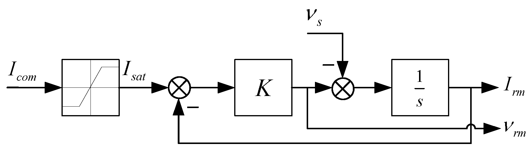
To overcome the effect caused by the actuator saturation, the pseudo-control hedging (PCH) scheme is adopted. The PCH solves the effect of actuator saturation by modifying the virtual control input instead of directly influencing the actuator input. When the input error signal of the control system is too radical for actuators, it allows the production of a signal ${\nu }_s$ which is opposite to the virtual control law to the first-order reference model, so that it can prevent the system from still trying to track the commanded references when actuator saturation occurs.

In order to achieve the control hedging, a first-order reference model is introduced as Figure 1. $I_{com}$ represents the command signal and $I_{sat}$ is the filtered signal to ensure the input is within the acceptable range of the system. ${\nu }_s$ is defined, corresponding to the input under the actuator dynamics. The maximum rate change allowed for this helicopter follows the ADS-33E-PRF standard, that is, the limits of 40 degrees per second on the roll and pitch rates and 80 degrees per second on the yaw rates. By using the reference model, we can obtain the time derivative of $I_{com}$ such that the virtual control $\nu$ in (4) can be made easily when no saturation occurs.

The PCH signal ${\nu }_s$ in the affine nonlinear systems can be calculated by

$$\begin{array}{l}{\nu }_s=\left[{\dot{x}}_0+G(x_0,u_0)(u_{des}-u_0)\right]-\left[{\dot{x}}_0+G(x_0,u_0)(u-u_0)\right]\\ =G(x_0,u_0)(u_{des}-u)\end{array}$$

(37)

where $u_{des}$ represents the desired actuator input, which can be produced by the rate controller.

4.3. Rate Loop

For the rate loop, it is expected that the helicopter can track the input angular rate signal in real time, which requires an error $e_{rat}$ to be defined between the reference signal and the system output, yielding

$$e_{rat}={\omega }_{des}-y_{rat}$$

(38)

where ${\omega }_{des}$ is the reference command which can be produced by the attitude controller. The rate of angular change between the body frame to the North–East–Down (NED) co-ordinate system $y_{rat}=x={\omega }_h={\left[\begin{array}{ccc}p& q& r\end{array}\right]}^T$ represents the angular rate output of helicopter.

Parallel to the INDI design procedure, we differentiate the output expression to obtain its explicit dependence on the actuator inputs $u$. This yields

$${\dot{y}}_{rat}={\dot{\omega }}_h=J^{-1}(m-{\omega }_h\times J{\omega }_h)$$

(39)

(39) can be rewritten as

$${\dot{y}}_{rat}={\dot{\omega }}_h=f_{rat}(x)+g_{rat}(x,u)$$

(40)

where

$$f_{rat}(x)=J^{-1}[m_{fus}(x)+m_{ht}(x)+m_{vt}(x)-\omega \times J\omega ]$$

(41)

$$g_{rat}(x,u)=J^{-1}\left[m_{mr}(x,u)+m_{tr}(x,u)\right]$$

(42)

Note that the number of actuators of the helicopter is four, which is not equal to the output state number in the rate loop. This means a control allocation scheme must be used to deal with this overdetermined system. However, because the change of the collective pitch of the main rotor, denoted by ${\theta }_0$, is always accompanied by the alteration of total lift, the value of ${\theta }_0$ can be determined by the velocity on the $z$-axis under the NED reference frame. Therefore, we separately give the control law of the main rotor in the subsequent design. Now, we define the other three actuators as $u^{\prime }={\left[\begin{array}{ccc}{\theta }_{1s}& {\theta }_{1c}& {\theta }_{0tr}\end{array}\right]}^T$.

Combining the analysis of the helicopter model before, we can obtain the rotational dynamics under actuator delay:

$${\dot{y}}_{rat}={\dot{\omega }}_h=f_{rat}(x)+g_{rat}(x,u_{\tau })$$

(43)

Choosing the virtual control ${\nu }_{rat}={\dot{\omega }}_{des}+k_{\nu r}{e}_{ret}$ with the control gain matrix $k_{\nu r}\in R^{3\times 3}$, the controller $u^{\prime }$ can be given by

$$u^{\prime }={u^{\prime }}_0+\Delta {u^{\prime }}_n+\Delta {u^{\prime }}_c$$

(44)

$$\Delta {u^{\prime }}_n=G_{rat}{(x_0,u_0)}^{-1}(\nu -{\dot{\omega }}_{h_0})$$

(45)

$$\Delta {u^{\prime }}_c=k_{ur}{G}_{rat}{(x_0,u_0)}^{-1}{\displaystyle {\int }_{t_0}^t\left[{\dot{e}}_{rat}+k_{rr}{e}_{rat}\right.}\left.+g_{rat}(x,u_{\tau })-g_{rat}(x,u)\right]d\theta$$

(46)

where $G_{rat}(x_0,u_0)=J^{-1}{\left.\frac{\partial }{\partial u^{\prime }}\left[m_{mr}(x,u)+m_{tr}(x,u)\right]\right|}_{x_0,u_0}$ and $k_{ur},k_{rr}\in R^{3\times 3}$ are also diagonal matrices. Note that there is a very complicated relationship between control input $u$ and the moment generated by the main rotor and tail rotor because of the aerodynamics of the rotors. Hence, we adopt the central finite differences to calculate the control effectiveness matrix denoted by $D$, yielding

$${\left.D=\frac{\partial }{\partial u^{\prime }}\left[m_{mr}(x,u)+m_{tr}(x,u)\right]\right|}_{x_0,u_0}=\left[\begin{array}{c}\frac{m_{mr}^T\left(x_0,{u^{\prime }}_0+{\left[\begin{array}{ccc}{\delta }_{{\theta }_{1s}}& \text{0}& \text{0}\end{array}\right]}^T\right)-m_{mr}^T\left(x_0,{u^{\prime }}_0-{\left[\begin{array}{ccc}{\delta }_{{\theta }_{1s}}& 0& 0\end{array}\right]}^T\right)}{2{\delta }_{{\theta }_{1s}}}\\ \frac{m_{mr}^T\left(x_0,{u^{\prime }}_0+{\left[\begin{array}{ccc}0& {\delta }_{{\theta }_{1c}}& 0\end{array}\right]}^T\right)-m_{mr}^T\left(x_0,{u^{\prime }}_0-{\left[\begin{array}{ccc}0& {\delta }_{{\theta }_{1c}}& 0\end{array}\right]}^T\right)}{2{\delta }_{{\theta }_{1c}}}\\ \frac{m_{tr}^T\left(x_0,{u^{\prime }}_0+{\left[\begin{array}{ccc}0& 0& {\delta }_{{\theta }_{0tr}}\end{array}\right]}^T\right)-m_{tr}^T\left(x_0,{u^{\prime }}_0-{\left[\begin{array}{ccc}0& 0& {\delta }_{{\theta }_{0tr}}\end{array}\right]}^T\right)}{2{\delta }_{{\theta }_{0tr}}}\end{array}\right]$$

(47)

where ${\delta }_{{\theta }_{1s}}$, ${\delta }_{{\theta }_{1c}}$, and ${\delta }_{{\theta }_{1c}}$ are a small percent of each actuator input value.

For actuator dynamics, a pseudo-control hedge command is generated to provide the control system from trying to track the reference command when saturation occurs. According to (37), the pseudo-control hedge command ${\nu }_r$ for the rate loop can be obtained by

$$\begin{array}{l}{\nu }_r=({\dot{x}}_0+J^{-1}D({u^{\prime }}_{des}-{u^{\prime }}_0))-({\dot{x}}_0+J^{-1}D(u^{\prime }-{u^{\prime }}_0))\\ =J^{-1}D({u^{\prime }}_{des}-u^{\prime })\end{array}$$

(48)

where ${u^{\prime }}_{des}$ represents the desired input vector produced by the rate controller.

After completing this, the whole rate-loop control system is accomplished. However, the helicopter still faces stability issues, for the reason that the Euler angle in the attitude loop is not closed-loop stable.

4.4. Attitude Loop

Then, for the attitude loop, we can use the NDI control on account of no model uncertainty existing here. In this loop, the system can be given by

$$\underset{¯}{\dot{\theta }}=\left[\begin{array}{ccc}1& \sin \varphi \tan \theta & \cos \varphi \tan \theta \\ 0& \cos \varphi & -\sin \varphi \\ 0& \sin \varphi /\cos \theta & \cos \varphi /\cos \theta \end{array}\right]{\omega }_h$$

(49)

$$y_{att}=x=\underset{¯}{\theta }={\left[\begin{array}{ccc}\varphi & \theta & \psi \end{array}\right]}^T$$

(50)

where $y_{att}$ represents the attitude angle output of the helicopter.

Unlike the rate loop, there is no model uncertainty or time delay in the attitude loop. Therefore, the attitude controller only needs to convert the attitude angle tracking error into the desired angular rate command as the inner loop input signal through the NDI method. Considering the state Equation (49), the reference input signal of rate loop ${\omega }_{ref}$ can be obtained by

$${\omega }_{ref}=\left[\begin{array}{ccc}1& 0& -\sin \theta \\ 0& \cos \varphi & \sin \varphi \cos \theta \\ 0& -\sin \varphi & \cos \varphi \cos \theta \end{array}\right]{\nu }_{att}$$

(51)

where ${\nu }_{att}$ is the virtual control for the attitude loop and it can be given by the attitude tracking error $e_{att}$ as

$${\nu }_{att}={\underset{¯}{\dot{\theta }}}_{des}+k_{\nu a}{e}_{att}$$

(52)

in which $k_{\nu a}\in {ℝ}^{3\times 3}$ is the control gain matrix and ${\underset{¯}{\theta }}_{des}$ is the attitude reference command for the helicopter. Note that the inverse of the transformation matrix always exists for $\det \Omega =1/\cos \theta \ne 0$.

In the attitude loop, the pseudo-control hedge command ${\nu }_a$ is

$${\nu }_a=\Omega ({\omega }_{ref}-{\omega }_h)$$

(53)

4.5. Control Law for Collective Pitch of Main Rotor

As mentioned in the rate loop, the operation of the collective pitch of the main rotor ${\theta }_0$ will change the lift of the helicopter directly. Hence, the actuator ${\theta }_0$ should be related to the vertical velocity of the helicopter. In the $z$-axis direction, the following equation is made

$${\dot{V}}_z-\mathrm{g}=\left[\begin{array}{ccc}-\sin \theta & \cos \theta \sin \varphi & \cos \theta \cos \varphi \end{array}\right]\frac{F}{m}$$

(54)

where $\mathrm{g}$ is the gravitational acceleration and $F={\left[\begin{array}{ccc}{F}_x& F_y& F_z\end{array}\right]}^T$ represents the total force in the three axes. It contains the contributions of all the main parts of the helicopter, yielding

$$F=F_{fus}+F_{ht}+F_{vt}+F_{mr}+F_{tr}$$

(55)

Once again, $F$ consists of the force produced by the fuselage, horizontal tail, vertical tail, main rotor, and tail rotor, respectively.

Note that, although the total force $F$ contains many parts, the main part is the force generated by the main rotor since it resists gravity while allowing the helicopter to move flexibly. Based on the assumption above, we can obtain the direct dependence about ${\dot{V}}_z$ to the delayed input ${\theta }_{0_{\tau }}$ as

$${\dot{V}}_z=g+\frac{1}{m}{\left[\begin{array}{c}-\sin \theta \\ \cos \theta \sin \varphi \\ \cos \theta \cos \varphi \end{array}\right]}^T{F}_{mr}(x,u_{\tau })$$

(56)

Choosing the virtual control ${\nu }_{vz}={\dot{V}}_{zdes}+k_{\nu z}{e}_{vz}$ with the control gain constant $k_{\nu z}\in R^{+}$, the controller for ${\theta }_0$ can be given by

$${\theta }_0={\theta }_{0,0}+\Delta {\theta }_{0,n}+\Delta {\theta }_{0,\mathrm{c}}$$

(57)

$$\Delta {\theta }_{0,n}=m{\left({\left[\begin{array}{c}-\sin \theta \\ \cos \theta \sin \varphi \\ \cos \theta \cos \varphi \end{array}\right]}^{T}H\right)}^{-1}({\nu }_z-{\dot{V}}_{z_0})$$

(58)

$$\Delta {\theta }_{0,\mathrm{c}}=k_{uz}m{\left({\left[\begin{array}{c}-\sin \theta \\ \cos \theta \sin \varphi \\ \cos \theta \cos \varphi \end{array}\right]}^{T}H\right)}^{-1}{\displaystyle {\int }_{t_0}^t\left[{\dot{e}}_z+k_{rz}{e}_z+F_{mr}(x,u_{\tau })-F_{mr}(x,u)\right]d\theta }$$

(59)

where ${\theta }_{0,0}$ also represents the previous sampling value of ${\theta }_0$; $k_{uz},k_{rz}\in R$ are positive control gains; and $H$ is the control effectiveness matrix, which can be expressed as

$$H={\left.\frac{\partial F_{mr}(x,u)}{\partial {\theta }_0}\right|}_{x_0,u_0}$$

(60)

It can also be calculated by using the central finite difference as

$$H={\left[\frac{F_{mr}{}^T(x_0,{\theta }_{0,0}+{\delta }_{{\theta }_0})-F_{mr}{}^T(x_0,{\theta }_{0,0}-{\delta }_{{\theta }_0})}{2{\delta }_{{\theta }_0}}\right]}^T$$

(61)

where ${\delta }_{{\theta }_0}$ is a small percent of ${\theta }_0$.

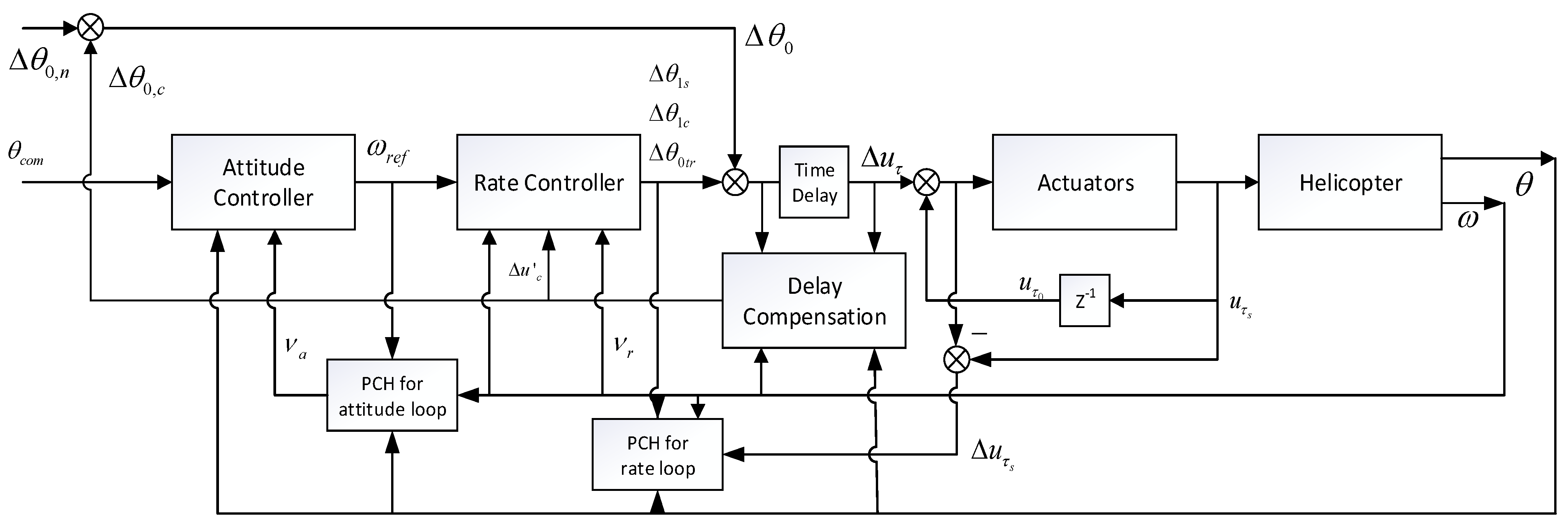
Now, the helicopter attitude control system under the multiple constraints of the actuators has been designed, which is shown in Figure 2.

5. Simulation Results

In this section, several simulations will be given to verify the advantages of the proposed control law. We will simulate the attitude control of the helicopter in a hovering state. The model uncertainties are given as $\Delta C_{L_{\alpha }}=-0.1C_{L_{\alpha }}, \Delta C_{L_{\alpha ,tr}}=-0.1C_{L_{\alpha ,tr}},$$\Delta C_{L_{\alpha ,ht}}=0.5C_{L_{\alpha ,ht}},$ and $\Delta C_{L_{\alpha ,vt}}=0.5C_{L_{\alpha ,vt}}$, where $C_{L_{\alpha }}$, $C_{L_{\alpha ,tr}}$, $C_{L_{\alpha ,ht}}$, and $C_{L_{\alpha ,vt}}$ are the lift curve slope of the blade of the main rotor, the blade of the tail rotor, the horizontal tail, and the vertical tail, respectively. The delay time is $\tau =100ms$, initial input $u_0={\left[\begin{array}{cccc}0.2484& 0.0275& -0.0135& 0.1289\end{array}\right]}^T$, diagonal element of control gain matrix $k_{ur}$ is ${\left[\begin{array}{ccc}1& 1& 1.5\end{array}\right]}^T$, and $k_{rr}$ is ${\left[\begin{array}{ccc}2& 2& 3\end{array}\right]}^T$.

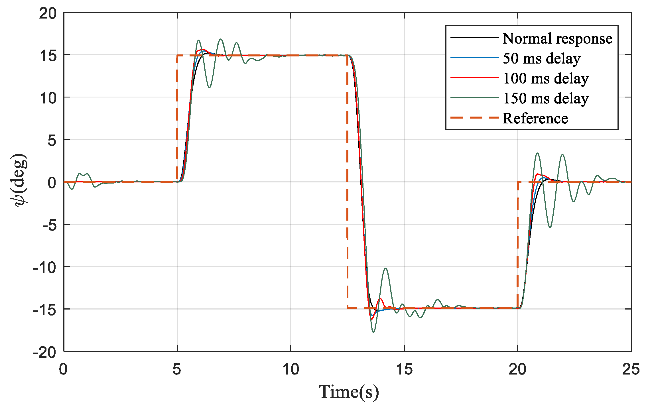
The delay of the actuators will degrade the tracking performance and increase the control effort provided by the actuators, which always leads to state overshoot and actuator saturation, and even causes the system to become unstable when the delay time gradually increases. This phenomenon can be observed in Figure 3.

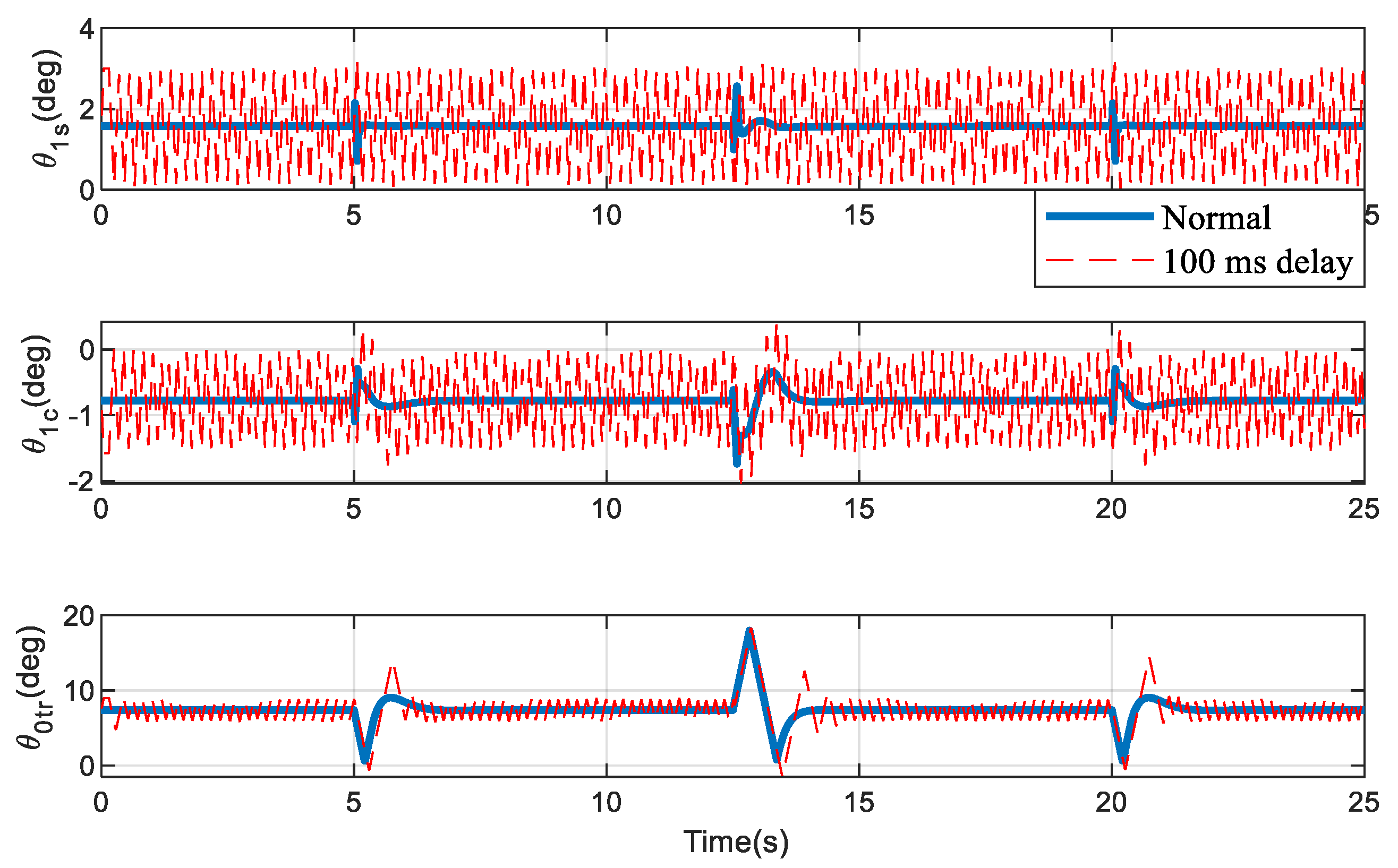
In this simulation, the operating frequency of the control system is set at 100 Hz. When the actuator delay is 50 ms, the INDI-based control system can barely maintain its tracking performance. A small range of oscillation appears in response when the delay time is 100 ms. However, actuators need to change frequency to maintain this steady state in the INDI scheme, which is shown in Figure 4. This can be understood as, when time delay exists, the control input does not correspond to the current input error, and it needs to be adjusted constantly within the whole time delay. In the case of the delay of 150 ms, the system response has already experienced a relatively large oscillation, and its dynamic characteristics are seriously degraded.

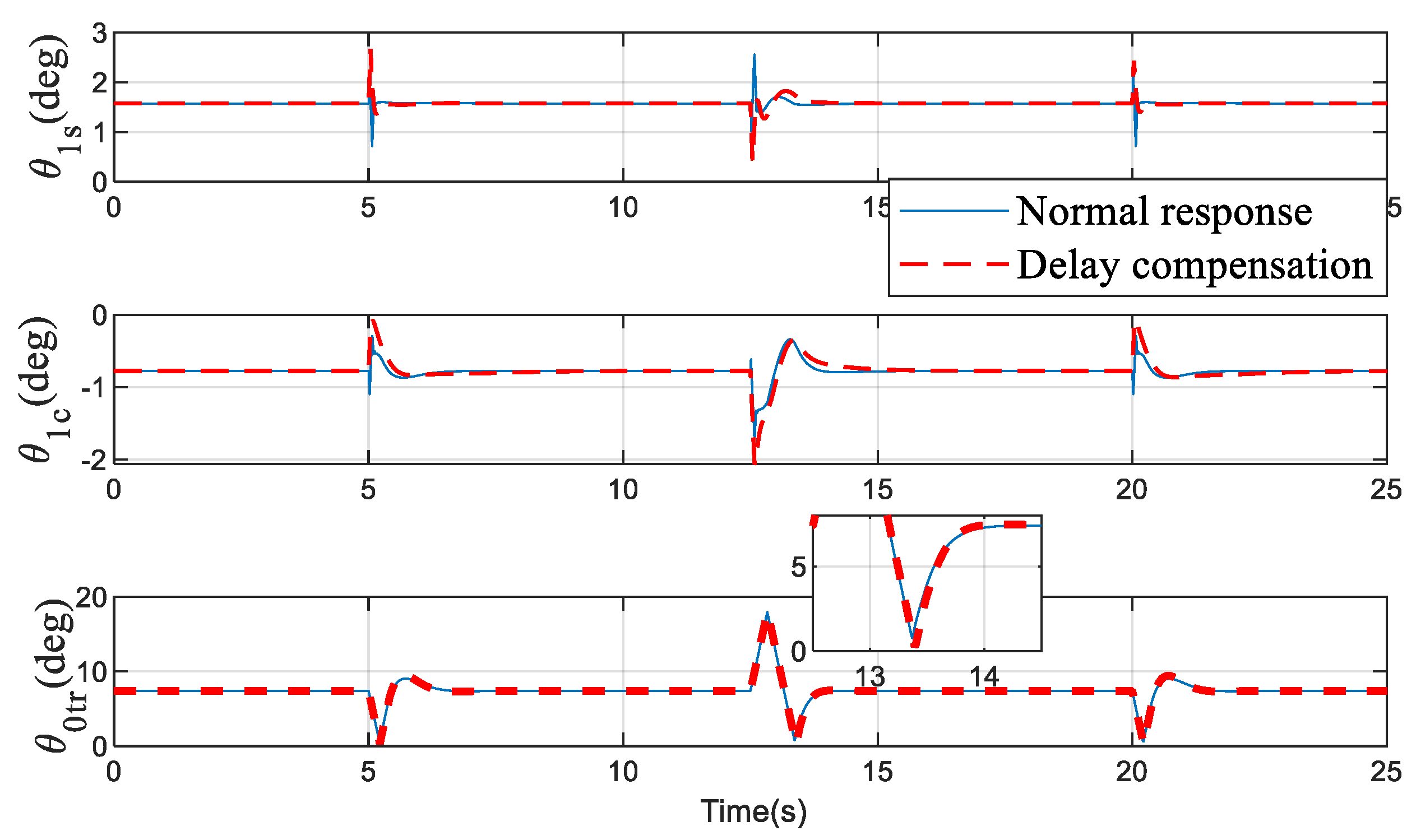
In the next simulation, the delay time between the controller and actuators is set at 100 ms. In Figure 5, it can be seen that, when the delay compensation is applied, the state overshoot is significantly reduced and the system’s rapidity is also improved compared to the original response. Figure 6 shows that, in addition to the need for a larger control effect, the original phenomenon of rapid changes has disappeared.

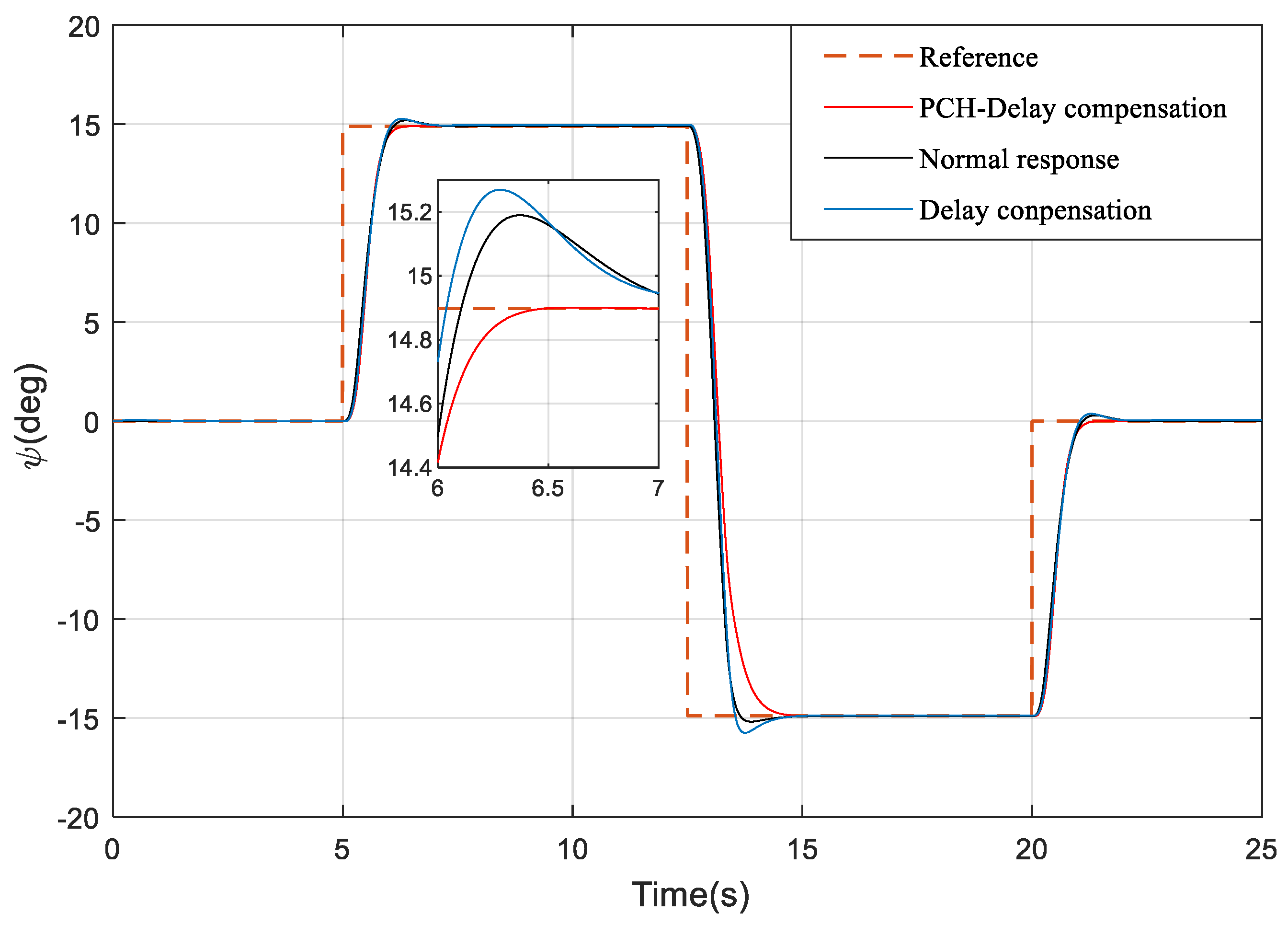
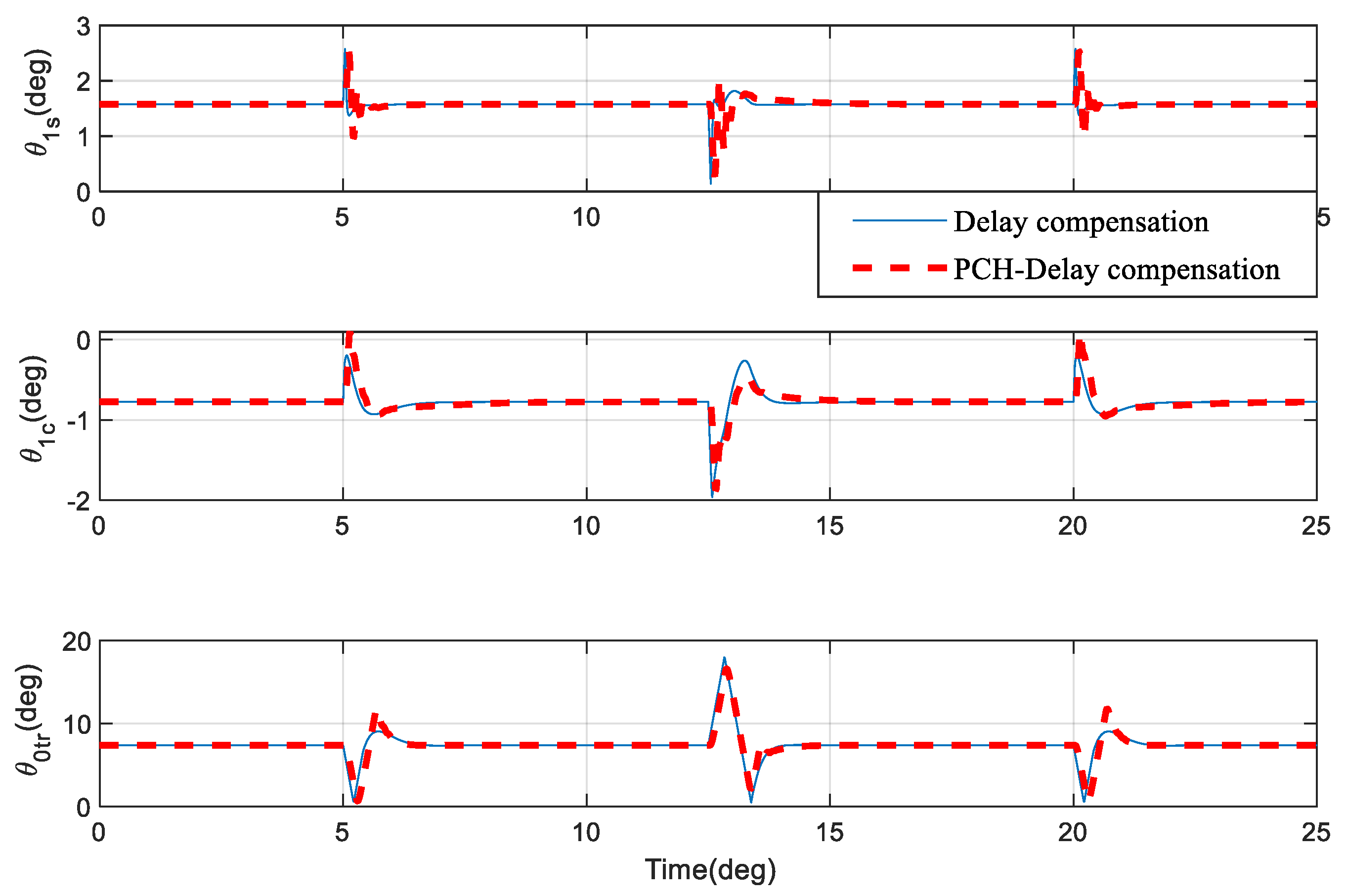
On the basis of delay compensation, we carry out the PCH design for the system. The advantages of PCH can be seen in Figure 7, which not only eliminates the overshoot, but also reduces the 0.7 s settling time of the system. Figure 8 is also given here to compare the changes of the actuators between the three cases.

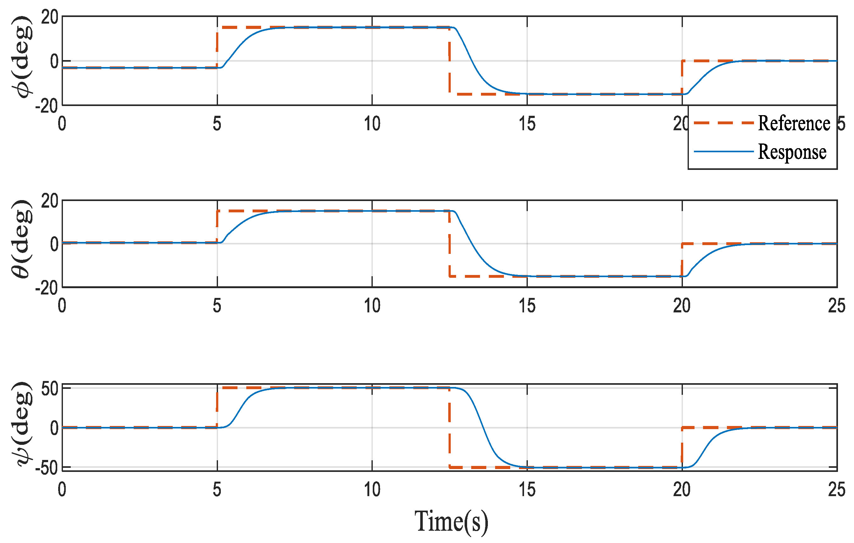
Finally, the response of the three channels of the attitude angle under the proposed control scheme is given in Figure 9. It can be seen that the three Euler angles can be decoupled and show good dynamic characteristics. In the Figure 10, the angular rates also change regularly corresponding to the tracking of the three Euler angular rates. Furthermore, the system can also track the command signal well when the actuator input is saturated and delayed, which can be observed in Figure 10.

6. Conclusions

In this paper, an INDI-based actuator compensation attitude controller is developed for the helicopter subject to the time delay, position, and rate saturations in actuators. The controller is composed of a rate controller which ensures the rate performance of the helicopter, an attitude controller which guarantees the attitude tracking performance, and a collective pitch controller which meets the needs of the vertical changes in the $z$-axis direction. The model reduction method is used to design an INDI-based controller for the rate loop and collective pitch of the main rotor, which improves the robustness to the time-varying actuator delay. Meanwhile, the PCH technique is introduced for both the rate loop and attitude loop to provide a filter such that the following commands hold within the capability of the controllers. Finally, simulations demonstrate the effectiveness and robustness of the proposed controller. In the future, the outer loop controller for the helicopter will be designed and a maneuver flight simulation analysis that meets the requirements of ADS-33E-PRF will be performed.