Article

A New Force Control Method by Combining Traditional PID Control with Radial Basis Function Neural Network for a Spacecraft Low-Gravity Simulation System

1
School of Mechatronics Engineering, Harbin Institute of Technology, Harbin 150001, China
2
Aerospace System Engineering Shanghai, Shanghai 201109, China
*
Authors to whom correspondence should be addressed.
Aerospace 2023, 10(6), 520; https://doi.org/10.3390/aerospace10060520
Submission received: 21 September 2022 / Revised: 12 May 2023 / Accepted: 26 May 2023 / Published: 1 June 2023
(This article belongs to the Section Astronautics & Space Science)

Abstract

:
With the continuous development of the space industry, the demand for low-gravity simulation experiments on the ground for spacecraft is increasing, to overcome the gravity compensation of spacecraft on the ground tests. This paper presents a new low-gravity simulation system based on the suspension method. We used a traditional PID control method with Radial Basis Function (RBF) neural network to solve its constant-tension control problem. The ant colony algorithm was used to find the initial parameters of the neural network in the solution space. A self-adjusting control strategy of PID controller parameters was realized. The results show that the tension control error of the low-gravity simulation system is as small as 0.2%, which fully meets the requirements of the system’s technical indicators. This work provides auspicious theoretical and technical support for developing a low-gravity simulation system.

1. Introduction

With the continuous development of science and technology, human beings pay more and more attention to research on space technology. All countries in the world hope to take the lead in making breakthroughs in space technology, so as to take the lead in the field of deep space exploration. Because the working environment of a spacecraft leaving the Earth is relatively harsh, researchers could not accurately grasp the spacecraft dynamics behavior in their practical work. Therefore, establishing an effective micro/low-gravity environment simulation system on the ground for the physical simulation of spacecraft will provide favorable conditions for space technology development [1,2]. In this article, in order to analyze the performance of high-precision mechanical devices with a mass of 10 to 100 kg in space, such as the motion and mechanical characteristics of small space robots in space, and the reliability of small and medium-sized equipment in space stations, a low gravity simulation system was established on the ground to simulate the low gravity environment in space.
According to the principle of realizing low gravity, a low-gravity ground simulation system’s compensation study can be divided into volume, area, and point force compensation [3].
Volume force compensation means that any micro unit of mass M in the spacecraft is subjected to a gravitational compensation force equivalent to Mg (Earth gravity). There are two typical methods of volume force compensation: the falling tower method and the parabolic flight method. The principle is to use the free-falling motion in the vertical direction to eliminate the influence of gravity temporarily.
The basic structure of the falling tower is the internal falling tank and the external tower body, as well as the lifting, releasing, decelerating, recovery, and other institutions. The gravity compensation accuracy of the typical German Drop Tower, Bremen, can reach 10−4 to 10−5 g (Earth gravity) [4]. A single simulation duration is about 4.74 s [5], which was improved to about 9.3 s [4]. The Japan Microgravity Center (JAMIC Drop Tower), the world’s largest, was built in the late 1980s [6]. It is 710 m underground and can provide 10 s of microgravity time at a microgravity level of 10−6 g, although it is not in operation currently [7].
The parabolic flight method obtains a short microgravity simulation time by keeping the horizontal velocity unchanged and the vertical acceleration zero when the aircraft is working [8,9]. The United States, Russia, and China mainly apply this technology, which can achieve a microgravity accuracy of 10−2 to 10−3 g, and a single parabolic flight lasts about 20 s. Although these two methods have high simulation accuracy, the single simulation time is short, and the preparation time of the experiment is prolonged, resulting in a high cost for the whole experiment.
Area force refers to the compensation force provided by the low-gravity system acting on the outer surface of the spacecraft. The resultant compensation force on these surfaces equals the spacecraft’s gravity. The method of area force compensation is mainly liquid float. The United States and Russia have built large underwater laboratories for astronaut training tasks [10]. NASA’s Johnson Space Center built the world’s largest underwater laboratory. Relying on this laboratory, NASA has conducted many experimental studies, such as the Hubble telescope repair simulation test [11] and the installation test of large parabolic precision reflectors [12]. The University of Maryland also successfully developed the Ranger system to conduct low-gravity simulation experiments for space robots [10]. Water float has the advantages of ample space, more degrees of freedom, and unlimited duration, but the target is often sealed, which increases the cost of the experiment. In addition, when the experimental target is moving, the water will produce relatively large resistance, which changes the dynamic behavior of the target.
Point force compensation is realized by applying a compensating force on the spacecraft to simulate low gravity, and the primary method is the suspension method and air float method. The United States, Japan, and Canada have conducted air-float-related research. The SSRMS (Space Station Remote Manipulator System) space manipulator developed by Canada, the JEMRMS (Japanese Experiment Module Remote Manipulator System) space manipulator developed by Japan, and the ERA (European Robotic Arm) space manipulator developed by ESA (European Space Agency) all used the air float method to conduct ground tests [13]. The air float method can significantly reduce the influence of friction. Still, because the high-pressure gas can only maintain the pressure in a small gap, the air float method cannot complete the gravity compensation in three-dimensional space, which has significant limitations.
The suspension method uses a sling to pull the experimental target and the tension from the sling achieves gravity compensation of the testing target. The suspension method can be divided into passive and active suspension methods according to whether the system contains an active driving device. The passive suspension method generally realizes gravity compensation through counterweight and pulley block structures. SM2 Space Manipulator Microgravity Simulation System GCI (Gravity Compensation I) and GCII (Gravity Compensation II), developed by Carnegie Mellon University in the United States, are composed of two-dimensional servo subsystems and counterweight gravity compensation subsystems to achieve low-gravity simulations. A low-gravity simulation system for astronaut walking and running developed by the University of California uses a treadmill, a pulley block, and multiple rubber springs to achieve minor tension fluctuation. The passive suspension method is easy to implement and low cost. However, additional mass is introduced due to the use of counterweights to provide tension. There is a lot of frictional interference in the mechanical structure, so it is mainly used in low-gravity simulations with large mass and low-gravity compensation accuracies, such as the deployment of spacecraft solar panels and space manipulator ground simulations.
The active suspension method follows the target and keeps the tension fluctuation on the sling within the allowable range by closed-loop control of the active element. The microgravity simulation system developed by Fujitsu is used to carry out the operation function verification experiment of a multi-joint space manipulator, and the accuracy can reach the order of 0.01 g. Texas A&M University has developed a dual-motor co-controlled constant-tension system that reduces the gravity error to 1% [14]. NASA has also developed several active gravity compensation systems to simulate low-gravity conditions on the Moon and Mars, contributing significantly to astronaut training and spacecraft ground simulation experiments [15].
In China, the Chinese Academy of Sciences uses FPGA to transfer the genetic control algorithm from software implementation to hardware implementation and uses it for PID parameter optimization, which improves the response speed of the system and suppresses overshoot.
In a comprehensive comparison, the active suspension method is simple, and the tension is adjustable. The simulation time and the size of the object are not limited. It can achieve multi-degree of freedom simulation. Therefore, this paper conducts the design of a low-gravity simulation system and constant-tension control research using the suspension method. Currently, the active suspension method has poor resistance to high-frequency disturbances and sudden force shocks, so elastic buffers are often added to suppress force shocks. However, adding a flexible link also reduces the bandwidth of the system, and the design of the system control algorithm becomes complicated. This paper designs a bypass-tensioning constant-force mechanism as a buffer device to improve the characteristics of the constant-tension system and meet the requirements of high bandwidth and high disturbance rejection control strategy.

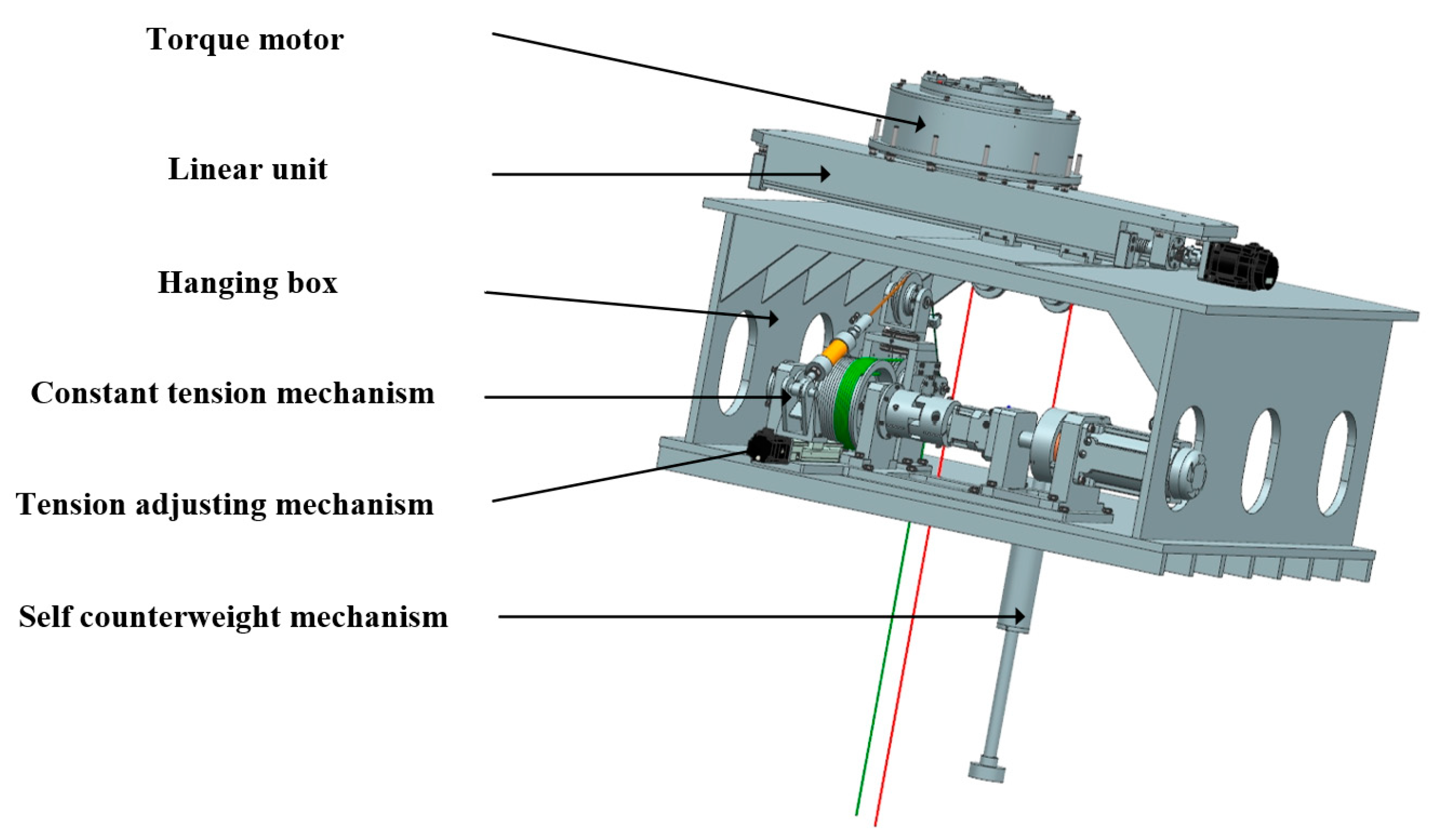
2. Low Gravity Simulation System Scheme

According to the technical indicators of the project, the mass range of the load is 10 to 100 kg, the maximum acceleration in the vertical direction of the load is 0.1 m/s2, the maximum speed in the vertical direction of the load is 0.3 m/s, and the number of lifting points is one. So, based on the load characteristics, the low-gravity simulation system is mainly composed of a constant-tension subsystem, a two-dimensional follow-up subsystem, and a control system. The essence of the constant-tension subsystem is to control the motor-driven sheave to retract and release the sling to follow the load movement and maintain the constant tension. The two-dimensional servo subsystem measures the inclination angle of the rope through the sensor, calculates the position of the center of mass to make the system follow, and keeps the rope vertical. The control system mainly communicates with each motor driver, limit switch, and various sensors to complete the closed-loop control. Three-degree-of-freedom gravity compensation is realized through integrated control of three systems. Figure 1 shows the overall scheme of the system.
According to the technical requirements, the tracking range of the two-dimensional servo subsystem is a hemispherical space with a radius of 300 mm. Therefore, we choose the motor to track the position of the load angle and change the tracking rotation radius through the linear motion pair of the ball screw, which can meet the needs of the motion trajectory. The linear unit adopts a structure consisting of four sliders on the double-track slide rail. By selecting high-precision slide rail and lead screw transmission pair, and controlling the processing and assembly accuracy of the support and installation benchmark, the rotating unit uses Renishaw circular grating as the angle measuring element, which can meet the requirements of motion accuracy.
When the servo subsystem works, in order to accurately track the centroid of the pointing mechanism, the control system will calculate the centroid position of the load according to the measured rotation angles of the load pitch axis and azimuth axis, control the motion of the rotary motor and linear motor, and track the centroid motion of the pointing mechanism.
Figure 2 shows the 3D structure of the whole low-gravity simulation system.
The low-gravity simulation system is mainly composed of a buffer mechanism and motor drive mechanism. When working, the torque motor outputs a specific torque after receiving the signal from the driver, drives the drum through the holding brake, reducer and other devices, and drives the sling in the buffer mechanism to retract and release, so as to realize the lifting, lowering and low-gravity simulation of the load.
The motor drive mechanism is mainly composed of a motor, brake, reducer, coupling, drum, and sling. The structure is shown in Figure 3.
The tension of the sling is detected by the force sensor in real-time and fed back to the control system to realize the closed-loop control of the tension, which can compensate the low-frequency interference of the system. However, it is difficult to use the control system to suppress the high-frequency change part of the tension caused by the movement of the turntable and the high-frequency change part of the friction caused by the motor commutation process. Therefore, an appropriate mechanical buffer and compensation mechanism must be designed to suppress it, providing the control system with the necessary response time and space.
The buffer mechanism is essentially an elastic link. Its function is to suppress high-frequency disturbance signals in the system and improve the control accuracy of sling tension. In order to achieve this function, elastic links are usually added to the system to reduce the equivalent stiffness of the sling. At present, the commonly used method is to directly connect the spring in series in the sling. This method is simple to realize. The lower the spring stiffness, the smaller the tension error on the sling, but the lower the spring stiffness, the greater the elongation, and the more likely the spring to resonate, so the actual application is subject to more restrictions. Therefore, the spring mechanism is used to tension the sling to keep the tension at all times. At the same time, the equivalent stiffness of the mechanism is reduced through reasonable mechanical structure design to reduce the tension fluctuation of the output within a certain stroke. The principles of these two devices are shown in Figure 4.
The buffer mechanism is a by-pass tension-type constant-force mechanism, which is composed of a swing rod, spring, and mechanical connecting device. The specific structure is shown in Figure 5. The swing rod is subject to tension spring, balance spring, and sling tension. At the initial moment, the torque of the swing rod is balanced. The swing rod is in the horizontal working position. When the tension fluctuates, the swing rod will rotate and apply tension to the sling.
The motor, linear unit, and spring seat in the figure are used to adjust the initial tension value of the tension spring. Since the mass range of the low-gravity simulation test load is 10~50 Kg, when the test piece is replaced, the load mass changes, so it is necessary to use the motor of the linear unit to adjust the position of the spring seat, change the initial tension of the tension spring, and make the swing rod return to the horizontal position. The code disk in the buffer mechanism is used to detect the angular position of the swing rod. The angle of the swing rod is between plus and minus ten degrees during normal operation. When the rotation angular displacement of the swing rod is too large, it is necessary to stop the experiment and check the cause.

3. Mathematical Modeling of Constant-Tension System

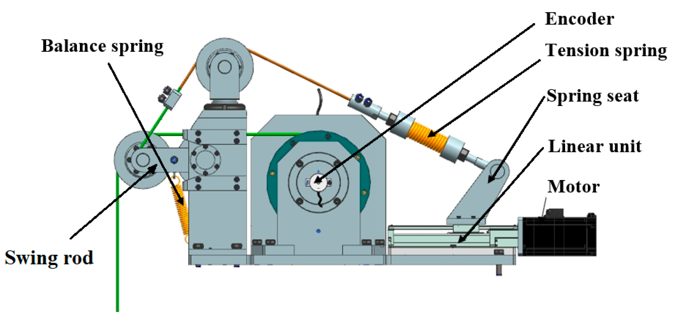
3.1. Modeling of the Buffer Mechanism

The specific structure of the buffer mechanism of the constant-tension system has been described in the previous article. The schematic diagram of its working position is shown in Figure 6. Taking the intersection point of the swing bar and the longitudinal bar as the origin O, an xg rectangular coordinate system is established. In the actual structure, the center of the drum and the origin of the coordinate system is not at the same point, but the sling between the two parts is only used to transfer the tension. Therefore, to simplify the model’s establishment, the center of the drum coincides with the origin O.
In the above Figure 6:
a is the center of the pulley.
b is the upper vertex of pulley 2.
c is the connection point between the left end of the pull spring and the pendulum rod.
d is the connection point between the right end of the pull spring and the bar.
e is the connection point between the left end of the balance spring and the pendulum rod.
f is the connection point between the right end of the balance spring and the longitudinal rod.
θ is the pendulum rotation Angle (rad).
T is the sling tension (N).
T1 is the tension on the spring (N).
T2 is the balancing tension on the spring (N).
Since the positions of points a, c, and e concerning the pendulum rod remain unchanged, the x b coordinate system with the straight line of the pendulum rod as its x axis is established, and the origin coincides with the origin of the x g coordinate system. Then the transformation matrix from the x b coordinate system to the x g coordinate system is
R b g = [ cos θ sin θ sin θ   cos θ ]
When the pendulum rotates at a certain angle θ, the coordinates of points a, c, and e in the x g coordinate system are as follows:
Coordinates of point A:
[ a x a y ] = [ cos θ sin θ sin θ   cos θ ] [ l a 0 ] = [ l a cos θ l a sin θ ]
Coordinates of point C:
[ c x c y ] = [ cos θ sin θ sin θ   cos θ ] [ l c l c y ] = [ l c cos θ l c y sin θ l c sin θ + l c y cos θ ]
Coordinates of point E:
[ e x e y ] = [ cos θ sin θ sin θ   cos θ ] [ l e l e y ] = [ l e cos θ + l e y sin θ l e sin θ l e y cos θ ]
Before the buffer mechanism works, it is necessary to adjust the position of point d according to the mass of the load so that the pendulum rod is initially in a horizontal state. Assuming that the tension spring’s original length plus the sling’s length is l0, when the low-gravity simulation system is working, the shape variable of the tension spring is | c b | + | b d | l 0 . According to Hooke’s Law, the tension on the tension spring is
T 1 = k 1 ( | o b o c | + | o d o b | l 0 ) o b o c | o b o c | = K 1 [ l c cos θ + l c y sin θ l b + l c sin θ l c y cos θ ]
where k1 is the stiffness coefficient of the tension spring (N/m). K1 is the equivalent stiffness of the tension spring (N/m):
K 1 = k 1 ( 1 + | b d | l 0 | o b o c | )
The balance spring is stretched when the pendulum rod is horizontal. Assuming that the original length of the spring plus the length of the sling is l2, then the shape variable of the spring is | e f | l 2 when the swing rod angle is θ, and the tension of the balance spring is
T 2 = k 2 ( | e f | l 2 ) o f o e | o f o e | = K 2 [ l e cos θ l e y sin θ l f + l e sin θ + l e y cos θ ]
where k2 is the balance spring stiffness coefficient (N/m). K2 is the equivalent stiffness of the balance spring (N/m).
K 2 = k 2 [ 1 l 2 | o f o e | ]
It is necessary to conduct dynamic modeling for the pendulum rod. The tension of the tension spring and the balance spring is decomposed to the X-axis and Y-axis. Figure 7 illustrates its torque calculation diagram.
Diagram: T1x is the component of T1 along the X-axis. T 1 x = K 1 l c cos θ + l c y sin θ
T1y is the component of T1 along the Y-axis. T 1 y = K 1 l b + l c sin θ l c y cos θ
T2x is the component of T2 along the X-axis. T 2 x = K 2 l e cos θ l e y sin θ
T2y is the component of T2 along the Y-axis. T 2 y = K 2 l f + l e sin θ + l e y cos θ
We write down the above equations for the rotation process of the pendulum rod and consider the damping in the swing process of the pendulum rod, and then the following dynamic equation can be obtained (counterclockwise rotation of the pendulum rod is positive) as follows:
J a θ ¨ = T l a cos θ + T 1 x | ( o c ) y | T 1 y | ( o c ) x | + T 2 x | ( o e ) y | T 2 y | ( o e ) x | η θ ˙ = T l a cos θ K 1 l b l c cos θ K 1 l b l c y sin θ + K 2 l f ( l e cos θ l e y sin θ ) η θ ˙
where Ja is the moment of inertia of the pendulum rod (kg·m2). η is the pendulum damping coefficient.
Therefore, the tension T on the sling can be expressed as
T = K 1 l b l c l a + K 1 l b l c y l a tan θ + J a l a cos θ θ ¨ K 2 l f l a ( l e l e y tan θ ) + η l a cos θ θ ˙
In practical work, the rotation angle θ of the pendulum rod is very small so that it can be linearized, including:
{ cos θ = 1 sin θ = θ
If the higher-order term of θ is small and can be ignored, then Equation (10) can be simplified as
T = K 1 l b l c K 2 l f l e l a + J a l a θ ¨ + η l a θ ˙ + K 1 l b l c y + K 2 l f l e y l a θ
When the swing rod is in a horizontal position, that is, when θ = 0 , it can be considered that the tension value of the sling at this time T p is the gravity of the load, and the tension fluctuation T caused by the rotation of the swing rod is the sling tension fluctuation, so
{ T = T p + Δ T T p = K 1 l b l c K 2 l f l e l a Δ T = J h θ ¨ + η h θ ˙ + K h θ
where J h is the equivalent inertia of the buffer mechanism k g · m 2 , J h = J a / l a . K h is the equivalent elastic coefficient of the buffer mechanism (N·rad) , K h = K 1 l b l c y + K 2 l f l e y / l a . η h is the equivalent damping of buffer mechanism, η h = η / l a .
The load mass can adjust the equivalent spring stiffness. The pendulum, T p , is equal to the gravity of the load when it is horizontal. We take a 50 kg load as an example to analyze the buffer mechanism.
The spring stiffness of the tension spring used by the buffer mechanism is 13 N/mm, the balance spring stiffness is 4.26 N/mm, the original length of the balance spring plus the sling length is 109 mm, and the equivalent spring stiffness of the balance spring is as follows:
K 2 = k 2 1 l 2 o f o e = 4.26 × 1 109 130 = 0.688 N / m m
According to Equations (6) and (13), when the weight of the object is 50 kg we have T = 490 N, K 1 = 2.506   N / m m .
Table 1 lists other parameters of the buffer mechanism. By substituting Equation (13), we can obtain the expression of the tension fluctuation T above the sling relative to the swing angle θ of the pendulum rod, as follows in Table 1.
{ J h = 0.154 ; η h = 3.846 ; K h = 68.92 Δ T = 0.154 θ ¨ + 3.846 θ ˙ + 68.92 θ
By substituting the value of Equation (14) into Equation (13), the transfer function of tension fluctuation on the sling to load acceleration can be obtained:
Δ T ( s ) y ¨ d ( s ) = K h + η h s + J h s 2 l a s 2 = 530.1 + 29.58 s + 1.18 s 2 s 2
According to the transfer function, the amplitude–frequency characteristic of the low-frequency buffer mechanism decreases at −40 dB/Dec, and the gain remains unchanged at a low value with the frequency increase. For 50 kg objects, the tension deviation of 1.2 N accounts for 24% of the thrust, so it is necessary to rely on the active control of the motor to compensate for the low-frequency interference. At high frequencies, the tension deviation caused by the same acceleration is 0.115 N so that the buffer mechanism can suppress the high-frequency interference of the system. In the actual work of the system, the acceleration signal is generally within 3 Hz so that the buffer mechanism can meet the requirements of use.

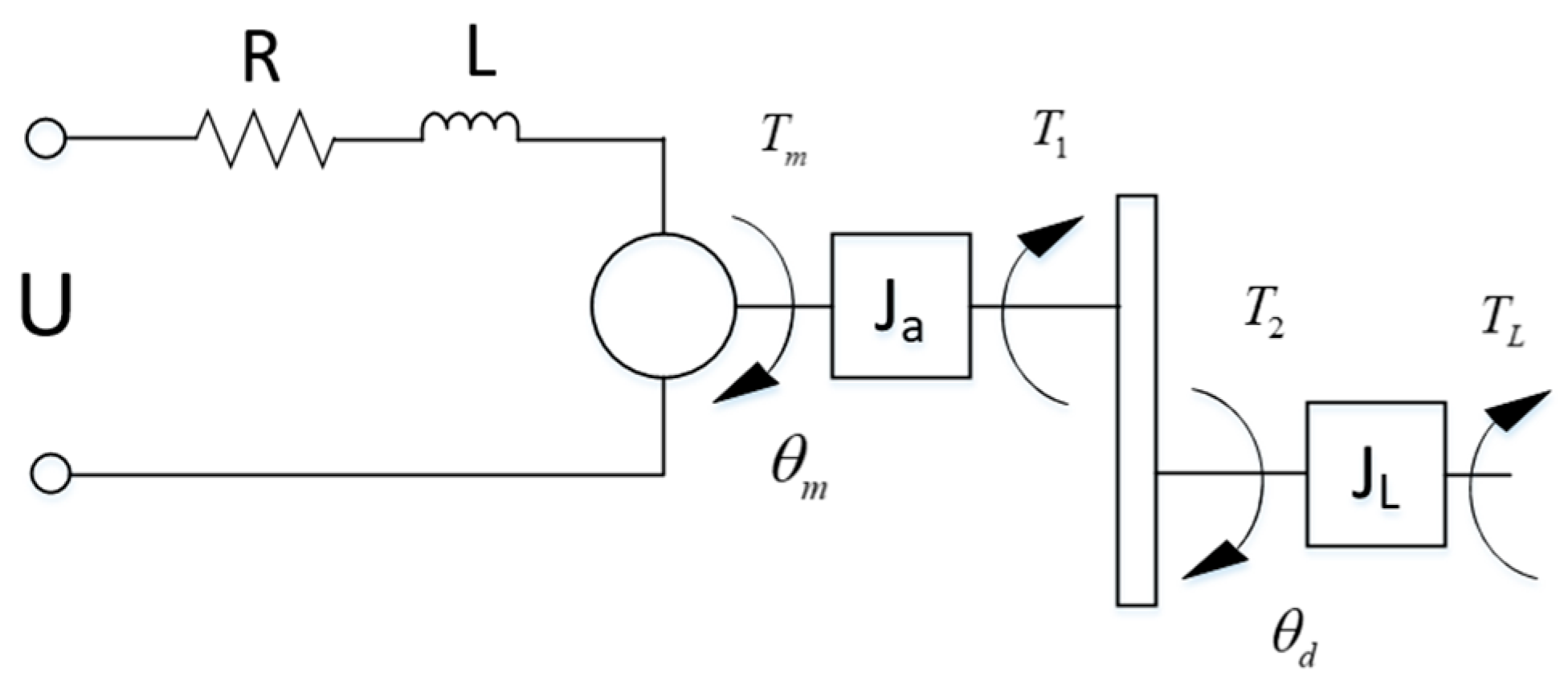
3.2. Overall Modeling of Constant-Tension System

The torque motor driving mechanism of the constant-tension control system is mainly composed of a torque motor, brake, reducer, and drum. The motor drives the drum to realize the retraction and release of the sling to compensate for the low-frequency interference force on the sling. Figure 8 shows the equivalent model of the mechanism.
In Figure 7, the armature loop of the torque motor can be equivalent to a resistance element plus an inductance element, and its dynamic characteristic equation is as follows:
U ( t ) = R i ( t ) + L d i ( t ) d t + K e d θ m ( t ) d t
where U is the motor input voltage (V). R is the total resistance of the armature loop (ω). L is the total inductance of the armature circuit (H). Ke is the motor equivalent back potential coefficient (Vs/rad). I is the armature loop current (A).
The motor input electromagnetic torque equation is
T m ( t ) = K t i ( t )
Tm is the motor output torque (Nm). Kt is the motor equivalent torque coefficient (N·m/A).
The constant-tension system is a motor-driving mechanism. Thus, the torque balance equation of the motor shaft and the output shaft of the reducer is
T m T 1 = J b d 2 θ m t d t 2 T 2 F × r = J L d 2 θ 1 t d t 2
For the reducer, the input torque is proportional to the output torque, and the proportional coefficient is its deceleration ratio, so there are
θ m = θ 2 × N T 2 = T 1 × N
where T1 is the reducer input torque (N·m). T2 is the reducer output torque (N·m). Jb is the moment of inertia of the motor rotor and reducer (kg·m2). F is the sling tension (N). R is the drum radius, r = 0.1 m. N is the reduction ratio of the reducer.
Based on the above formula, the total torque balance equation of the direct drive mechanism can be obtained as follows:
T m = J b d 2 θ m t d t 2 + 1 N J L N d 2 θ m t d t 2 + F · r = J d 2 θ m t d t 2 + T L
where J is the equivalent moment of inertia of the direct drive mechanism to the motor shaft,  J = J b + J L N 2 = 0.04 k g · m 2 . TL is the Load torque generated by sling tension (N·m).
Thus, the transfer block diagram of the direct drive mechanism can be obtained, as shown in Figure 9.
Table 2 lists the relevant parameters involved in Figure 8.
We have analyzed the buffer mechanism and direct drive mechanisms’ mathematical models separately. To establish the overall model of the constant-tension system, we also need to combine the dynamic characteristics of the load to obtain a complete model.
Take the upward movement of the load as the positive direction of y d , the counterclockwise rotation of the pendulum rod as the positive direction of θ , and the winding line of the drum as the positive direction of the rotation angle of the drum θ d . Then the relative relationship equation between the three variables is
y d = θ d r l a sin θ
After linearization, we can obtain:
y d = θ d r l a θ
That is,
θ = 1 l a ( θ d r y d )
By combining the mathematical model of the buffer mechanism and direct drive mechanism mentioned above, the transfer block diagram of the whole constant-tension system without a controller can be obtained, as shown in Figure 10.
The open-loop transfer function of sling torque on motor voltage can be obtained from the transfer block diagram. It is as follows:
T L ( s ) U ( s ) = r 2 K T L J h s 3 + r 2 K T ( R J h + L η h ) s 2 + r 2 K T ( R η h + L K h ) s + r 2 K T R K h A 1 s 4 + A 2 s 3 + A 3 s 2 + A 4 s + A 5
Among them
{ A 1 = l a L 2 J + r 2 L 2 J h A 2 = l a R L J + r R L J h + l a L R J + r 2 L R J h + L 2 r 2 η h A 3 = l a L K T K e + r 2 L R η h + r 2 L 2 K h + l a J R 2 + r 2 R 2 J h + r 2 L R η h A 4 = r 2 L R K h + l a R K T K e + r 2 R 2 η h + r 2 R L K h

3.3. PID Control System Construction

PID control is one of the most commonly used control laws in classical control methods, and has the characteristics of simple structure, robustness, strong adaptability, and high reliability.
However, how to determine the proportional, integral, and differential parameter values according to the characteristics of the controlled system is the key to PID control. At present, the methods of PID parameter tuning can be divided into two categories. The first category is to calculate the controller parameters according to the accurate mathematical model of the system. However, the current control system with load has many nonlinear factors, which are difficult to apply directly; the second is the engineering setting method, which is adjusted according to engineering experience.
In this paper, the Z-N critical proportional method is used to adjust PID parameters. First, the stability limit of the system is found by adjusting the value of proportional parameters, and then the parameter value of PID is calculated according to the formula. The calculation method is
{ k p = 0.6 K n k i = 1.2 K n T c k d = 0.072 K n T c
where Kn is the gain when the system is in critical oscillation and
Tc is the oscillation frequency when the system is in critical oscillation.
The value obtained by adopting the Z-N setting method and properly adjusting PID parameters are
k p = 5 ,   k i = 30 ,   k d = 0.002
Taking a 50 kg load as an example, to counteract the influence of gravity, the sling tension should be 490 N. Therefore, the system model is built into the simulation software, and the parameters are brought in. The smooth step signal is input. The system response obtained is shown in Figure 11. From Figure 11, it can be seen that the system reaches a stable state within 1.5 s and the steady-state error is zero. Before reaching the steady-state state, the system has a certain overshoot, and the maximum tensile force is around 540 N.

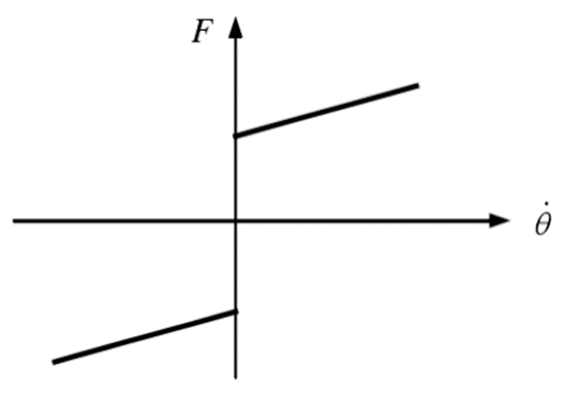
3.4. Influence of System Friction on Constant-Tension Control

Friction is a very complex and nonlinear physical process, and there is still no accurate mathematical expression to describe this process. In the above section, we chose to ignore the effect of friction. However, to improve the accuracy of the constant-tension system model and the persuasiveness of the subsequent control algorithm, the friction model widely used in engineering applications will be added to the simulation to describe the influence of friction on the system. Considering that the friction in the constant-tension system is mainly Coulomb friction plus viscous friction, the Coulomb viscous friction model is selected, and the friction model is shown in Figure 12.
The Coulomb friction in Figure 11 is a constant value which has nothing to do with the movement speed of the system. Coulomb friction is taken as 2 Nm, and viscous friction is related to the lubrication liquid phase versus sliding, so viscous damping coefficient B = 0.05 N·m·s/rad. As shown in Figure 13, the constructed model was added to the motor model, and the system response curve was obtained in the simulation software. Figure 14 illustrates the comparison with the response curves with and without friction.
From Figure 13, it can be seen that friction mainly affects the system in the low-speed operating region and has little influence when the rotational speed increases. After the introduction of friction, the maximum tension fluctuation of the system is 2.4 N after the interference signal of load acceleration, and the transition time is about 1 s, while the system provides 0.1 m/s2 for a 50 kg load. The driving force required for acceleration is only 5 N, and the tension fluctuation accounts for 48% of the driving force, seriously affecting the system’s performance.

3.5. Influence of Motor Torque Fluctuation

A torque motor drives the constant-tension system. The system requires the maximum load mass of the motor compensating gravity to be 50 kg, and the order of magnitude of tension control accuracy is 1 N. Therefore, although the non-ideal factor of torque motor characteristics is not large relative to its rated output, it still affects the force control accuracy of the system.
The output torque fluctuation of the torque motor is a complex process, mainly affected by electromagnetic, commutation, and groove effects [16]. This paper uses white noise in the simulation platform to simulate the torque fluctuation. The correlation time of white noise is 0.005 s, and the spectral density is 0.0003 N m 2 s / r a d . Figure 15 shows the obtained torque fluctuation signal.
After adding the torque fluctuation signal, the system response curve can be obtained, as shown in Figure 16. Compared with the response curve under friction only, the variation trend of tension is consistent. Still, there will be a fluctuation of about 0.3 N on this basis.

3.6. Impact of Load Acceleration Interference

In the low-gravity simulation experiment, after the constant-tension system reaches a steady state, the operator will drive the ground turntable to move and carry out a series of ground simulation experiments. When the constant-tension system is disturbed by the acceleration of the load, it will follow the load and keep the tension constant. Therefore, in the simulation, we give the system a value of 0.1 m/s2 Step acceleration signal at 3 s. In the existing system, the acceleration of the load will fluctuate around 0.1 m/s2 due to the influence of many factors, including frame vibration and torque fluctuation. Therefore, we added band-limited white noise.
Figure 17 shows the tension response curve of the sling after being disturbed by load acceleration. It can be seen that the tension error caused by the low-frequency signal in acceleration remains at about 0.8 N after the response of the motor. After the high-frequency part of the acceleration is suppressed by the buffer mechanism, the tension fluctuation caused by it is minimal, which does not affect the low-gravity simulation experiment. This is also consistent with our previous analysis of the buffer mechanism.

4. Controller Design of Constant-Tension System

4.1. Feed-Forward Compensation for Acceleration Interference

When modeling the constant-tension system, we take the ideal tension value as the system input, the actual tension value of the sling as the system output, and the acceleration signal of the load as the system interference. As can be seen from Figure 16, for the high-frequency part of the acceleration signal, after the passive suppression of the buffer mechanism, the impact on the tension control is very small and can be ignored; for the low-frequency part of the acceleration signal, although a PID controller is designed to control the active compensation of the motor, due to the system inertia and other factors, under the step acceleration signal of 0.1 m/s2, the sling tension has a steady error of about 0.8 N. In order to further improve the control accuracy of the constant-tension system, we use the feed-forward correction link to compensate for the interference.
Figure 18 shows a block diagram of a control system with interference, where R s is the ideal signal input by the system, a s is the system interference signal, and y s is the sling tension output of the system. G 1 s is the transfer function between the interference point and the error signal point, and G 2 s is the transfer function between the interference point and the feedback point.
To analyze the influence of the interference signal on the system output, we assume that the system input signal R s is zero. Then the system output y s generated by the interference a s is
y ( s ) = G 2 ( s ) 1 + G 1 ( s ) G 2 ( s ) a ( s )
Since the system output is zero, then due to interference, the error signal at the output of the system is
E n ( s ) = 0 y ( s ) = G 2 ( s ) 1 + G 1 ( s ) G 2 ( s ) a ( s )
According to the final value, the steady-state error of the system is
e s s n = lim s 0 s E n ( s ) = lim s 0 s G 2 ( s ) 1 + G 1 ( s ) G 2 ( s ) a ( s )
At present, disturbance observer, active disturbance rejection control, system correction, and other methods have been used to compensate for steady-state errors caused by interference signals. Because the acceleration interference signal of the load in the system can be measured by the sensor, aiming at this characteristic, this paper adopts the feed-forward correction link in system correction to compensate for the interference signal and improve the control precision of the constant-tension system.
As shown in Figure 19, a feed-forward correction link G n s is added between the interference signal and the error signal point, so the response of the system output to the interference signal after the correction link is introduced is
y ( s ) = G 2 ( s ) [ 1 + G 1 ( s ) G n ( s ) ] 1 + G 1 ( s ) G 2 ( s ) a ( s )
It can be seen from the above formula that, if setting 1 + G 1 s G n s = 0 , the output of the system under the interference signal is
E n ( s ) = y ( s ) = G 2 ( s ) [ 1 + G 1 ( s ) G n ( s ) ] 1 + G 1 ( s ) G 2 ( s ) a ( s ) = 0
Thus, it can be concluded that the conditions for complete compensation of interference signals are as follows:
G n ( s ) = 1 G 1 ( s )
In practical systems, the order of the denominator of G 1 s is usually higher than the numerator, so it is challenging to compensate entirely for the interference signal. However, approximate compensation can be achieved in the main frequency band of the interference signal by adjusting G n s , and most of the steady-state errors can be compensated.
Figure 20 is the constant-tension control structure diagram of the nominal system model. There are two local negative feedbacks for θ d and T L . It is not conducive to our analysis of the system structure and design of the feed-forward correction link. So, we use the movement of the addition point and the equivalent replacement of the local negative feedback to simplify the system’s constant-tension control block diagram and add a feed-forward correction link. The structure is shown in Figure 21, Where G 1 s is the transfer function after the equivalent replacement of T L local negative feedback. Since it does not affect the design of the feed-forward correction link, its specific expression is not given here.
The output of the feed-forward correction link can be added before or after the controller. However, due to the mass range of the load of the constant-tension system ranging from 10 to 50 kg, the controller parameters may change according to different loads, so we choose to add the output of the correction link after the controller.
Assume that the transfer function of the feed-forward correction link is G H s = G N s s 2 . According to Equation (29), it can be found that the conditions for realizing complete compensation for interference are
G n ( s ) = 1 / ( K T L s + R × L s + R L J s 2 + R J s + K T K e × r s ) = s ( L J s 2 + R J s + K T K e ) K T r
Namely, the transfer function of the feed-forward correction link is
G H ( s ) = G N ( s ) s 2 = L J s 2 + R J s + K T K e K T r s
Since the acceleration signal contains a high-frequency interference signal, the high-order differential term in the molecule will amplify the error of noise, so we ignore L J s 2 in the molecule, and the final feed-forward correction transfer function is
G H ( s ) = R J s + K T K e K T r s
In the simulation, the feed-forward correction was added to the model. Other nonlinear factors were ignored, the acceleration interference signal was set as 0.1 m / s 2 step signal, and acceleration signal noise were added. Figure 22 shows the system response curve after introducing feed-forward correction. It can be seen that the low-frequency part of the acceleration interference signal has been completely compensated.
In practice, the acceleration signal of the load is generally in the form of sines and cosines, and the frequency is within the range of 3 Hz. Therefore, the acceleration signal is changed to the sinusoidal frequency sweep signal from 0 to 3 Hz in the simulation model. Figure 23 shows the obtained system response curve under a sinusoidal frequency sweep signal. As seen in Figure 23, the tension error increases with the increase of frequency. This is caused by the neglect of the differential term of the feed-forward link. In general, the error after compensation is no more than 0.01 N, which does not influence the work of the constant-tension system.

4.2. Adaptive PID Control Based on RBF Neural Network Identification

A constant-tension system is a complex control system with strong nonlinearity. Meng Duan et al. designed a fast terminal sliding mode controller for this challenging situation. However, it may not be easy to achieve in the industry [17], so the PID controller is chosen as the controller structure of the main loop in this paper. Although the influence of load acceleration interference signal on the system is suppressed by feed-forward correction control, the performance of the PID controller does not meet our requirements in the face of friction, torque fluctuation, and other factors. Therefore, the PID controller must be improved.
This section proposes to combine the PID control strategy with RBF neural network. According to the adaptive characteristics of the neural network, PID parameters are adjusted online to improve the robustness of the system. The ant colony algorithm is used to find the initial parameters of the neural network in the solution space to enhance the efficiency of the neural network. At the same time, according to the PID control strategy with a dead zone, the learning rules of the integral term parameters are improved to solve the problem of system oscillation caused by excessive integral term parameters.

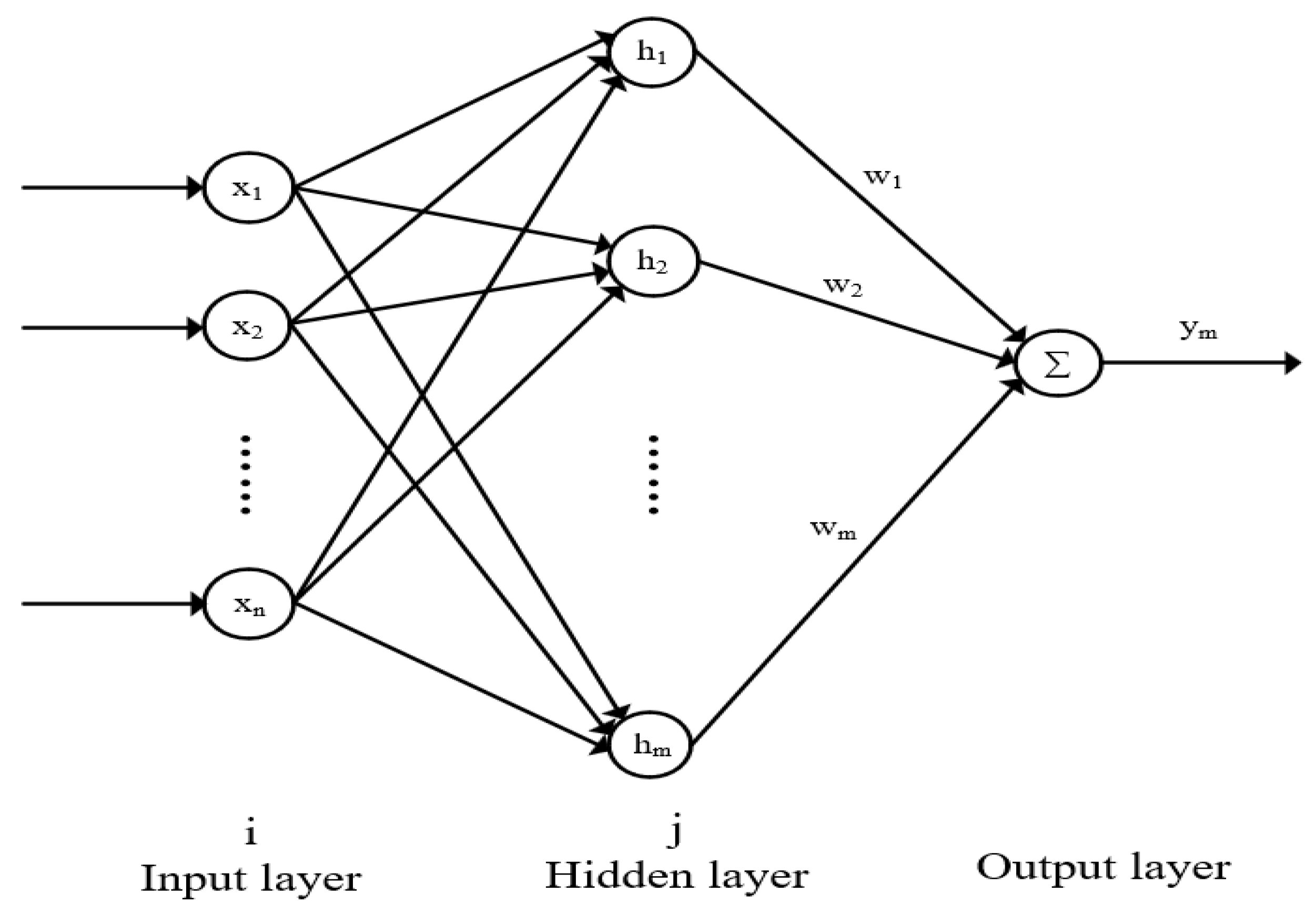
4.2.1. RBF Network Structure and Learning Algorithm

RBF neural network, also known as radial basis neural network, is a three-layer feed-forward neural network with a single hidden layer, a local approximation neural network. It can approximate any nonlinear function with arbitrary precision and has significant advantages in convergence speed and avoiding local fitting [18].
Figure 24 is the structure diagram of the RBF neural network, which is divided into three layers: input layer, hidden layer, and output layer. The number of neurons in the input layer is determined by the dimension of the input vector X = x 1 , x 2 , , x n . The number of neurons in the hidden layer is set according to the system’s needs, and the radial basis vector of the hidden layer H = h 1 , h 2 , , h j , , h m , where h j is the radial basis function, and the radial basis function is adopted in this paper in the form of the Gaussian basis function, so
h j = exp ( X C j 2 2 b j 2 ) ( j = 1 , 2 , , m )
where C j = c j 1 , c j 2 , , c j n is the center vector of the jth neuron in the hidden layer, b j is the base width parameter of the jth neuron in the hidden layer, and B = b 1 , b 2 , , b m is the base width vector of the network. The output of the network is y m , so:
y m = w 1 h 1 + w 2 h 2 + w m h m
where W = w 1 , w 2 , , w m is the weight vector from the hidden layer to the output layer, and w j is the connection weight of the jth neuron in the hidden layer.
Generally, the number of hidden layers in the RBF neural network is unchanged. So, the parameters that need to be learned and adjusted in the network mainly include the center vector of each neuron in the hidden layer, the base width vector, and the connection weight between the hidden layer and the output layer. When the RBF neural network identification system is used, the learning rule is supervised learning with teacher signals. That is, if the actual output of the system is y and the network output is ym, then the performance indicators of the discriminator are
J = 1 2 ( y ( k ) y m ( k ) ) 2
According to the gradient descent method to adjust the parameters, the learning algorithm is as follows:
w j ( k ) = w j ( k 1 ) + η ( y ( k ) y m ( k ) ) h j + α ( w j ( k 1 ) w j ( k 2 ) )
Δ b j = ( y ( k ) y m ( k ) ) w j h j X C j 2 b j 3
b j ( k ) = b j ( k 1 ) + η Δ b j + α ( b j ( k 1 ) b j ( k 2 ) )
Δ c j i = ( y ( k ) y m ( k ) ) w j x j c j i b j 2
c j i ( k ) = c j i ( k 1 ) + η Δ c j i + α ( c j i ( k 1 ) c j i ( k 2 ) )
where η is the learning rate, and α is the momentum factor. The learning rate and momentum factor values of different parameters can be different.
Take the input of the controller as the first value of the input vector of the neural network, then x 1 = u k , the Jacobian information of the object (the sensitivity of the output of the object to the input) is
y k u k j = 1 m w j h j u k = j = 1 m w j h j c j 1 x 1 b j 2

4.2.2. RBF Network PID Parameter Setting Principle

Figure 25 shows the structure of the PID self-tuning control system based on RBF system identification.
The PID controller in the figure above is incremental PID control, which calculates the increment of each controller output. The control error is
e ( k ) = r i n ( k ) y o u t ( k )
The input of the controller is
{ x c ( 1 ) = e ( k ) e ( k 1 ) x c ( 2 ) = e ( k ) x c ( 3 ) = e ( k ) 2 e ( k 1 ) + e ( k 2 )
The control algorithm of the incremental PID controller is as follows:
u ( k ) = u ( k 1 ) + k p ( e ( k ) e ( k 1 ) ) + k i e ( k ) + k d ( e ( k ) 2 e ( k 1 ) + e ( k 2 ) )
Let the setting index of the PID parameter be
E ( k ) = 1 2 e ( k ) 2
According to the gradient descent method, the adjustment rule of kp, ki, and kd is
{ Δ k p = η p E k p = η p E y y Δ u Δ u k p = η p e ( k ) y Δ u x c ( 1 ) Δ k i = η i E k i = η i E y y Δ u Δ u k i = η i e ( k ) y Δ u x c ( 2 ) Δ k d = η d E k d = η d E y y Δ u Δ u k d = η d e ( k ) y Δ u x c ( 3 )
where η p , η i , and η d are the learning rates of proportion, integral, and differential, respectively.

4.2.3. Initial Parameter Determination of Network Based on Ant Colony Algorithm

When RBF neural network is used as a system identifier, the initial network parameters to be determined mainly include the center vector b j and base width parameters C j of each neuron in the hidden layer, the initial weight w j from the neuron in the hidden layer to the neuron in the output layer, and the learning rate η and momentum factors α of each parameter. Among them, the determination of learning rate and momentum factors is not complicated, but there is no complete rule to determine the initial value of C j b j w j . In order to improve the accuracy of network identification, an ant colony optimization algorithm is adopted in this paper to search the initial values of these three parameters to select appropriate initial values for subsequent simulation.
We summarize the initial parameter optimization process of the RBF neural network based on the ant colony algorithm in the following steps:
(1) Construct solution space
According to experience, the approximate range of initial parameters in the RBF network is estimated, and parameter optimization is carried out within this range. In this paper, the network input is X = u k , y k , y k 1 . Therefore, the upper and lower bounds of the center vector of the hidden layer neuron are set as 30,50,50 and 30,10,10 , respectively. The upper and lower bounds of the base width parameter are 20 and 0.1, respectively, and the upper and lower bounds of the weight value from the hidden layer to the output layer are ±2.
(2) Determine the fitness expression
Fitness selection is the error between the RBF network identification output and the actual system output, expressed as:
f i t n e s s ( i ) = | y o u t y m o u t |
where y o u t is the output of the system, and y m o u t is the output of the neural network identifier.
(3) Calculate the probability of state transition
It is expected to conduct a local search near the current value for ants with good fitness. While it is expected to perform a random search in the global space for ants with poor fitness. This paper determines the probability of state transition as follows:
P ( i ) = f i t n e s s ( i ) min ( f i t n e s s ) max f i t n e s s ( i ) min ( f i t n e s s )
P i is the state transition probability of the ith ant.
(4) Update ant location
When the state transition probability of the ith ant is less than the state probability constant, it is made to do a local search near the current position to find the optimal solution. The search formula is
n e w = o l d + ( 2 × r 1 ) × λ
where r is a random number between 0 and 1, λ = 1 / 10 + T is the local search step, and T is the number of iterations.
When the state transition probability of the ith ant is greater than the constant state probability, it is made to search globally in the solution space. The search formula is
n e w = o l d + U p p e r B o u n d l o w e r b o u n d × r 0.5
(5) Judge whether to continue the iteration
After completing step (4), if the fitness meets the requirements or the number of iterations reaches the set maximum number of iterations, the search will be stopped. Otherwise, steps (2), (3), (4), and (5) will be mechanically repeated.
Set the number of ants to 50 and randomly put them into the solution space with ten iterations. The searched parameters are put into the simulation model. The obtained RBF network identification curve and the actual output curve of the system can be obtained, as illustrated in Figure 26. The acquired system Jacobian information is shown in Figure 27.

4.2.4. RBF Neural Network PID Control Simulation

In the simulation software, the incremental PID controller of the RBF neural network is built by modules. The number of neurons in the input layer of the RBF neural network is 1, and the number of neurons in the output layer is 6. The input vector of the network is X = [Δu(k), y(k), y(k−1)], the output is ym(k), the results of the parameter values of the hidden layer are substituted into the ant colony algorithm, with neural network parameter learning rate η = 0.2 and momentum factor α = 0.05. The learning rate of PID parameters is ηp = 100, ηi = 20, ηd = 100, and the parameters after the analog PID controller is converted into incremental PID control are kp = 5, ki = 0.03, ηd = 2.
Since the error of the constant-tension system is too large in the static equilibrium stage, PID parameter adjustment is not carried out at this stage, friction is added to the model, and the influence of motor torque fluctuation is not taken into account. Figure 28 and Figure 29 show the system response curve and PID parameter setting curve obtained, respectively. It can be seen from the figure that under RBF-PID control, the system deviation caused by friction is significantly reduced, and the deviation is controlled within 1 N and rapidly attenuates within 0.5 s, which can meet the requirements of technical indicators of a constant-tension system.
According to Equation (46), the learning rule of an integral term is
Δ k i = η i E k i = η i y Δ u e 2 ( k )
Introducing the integral term in PID control aims to eliminate static error. Still, due to the fluctuation of motor torque, there is always some error in the constant-tension system. The error caused by the torque fluctuation will make the PID controller act frequently. According to Equation (52), when the Jacobian information y u of the system is positive, the parameter value of the integral term always increases. Still, the parameter value of the integral term is too large to lead to system oscillation or even divergence quickly. After the introduction of torque fluctuation, the response curve of the integral term with a learning rate of 20 and the parameter setting curve of the integral term can be obtained, as shown in Figure 30. It can be seen that the accumulation of integral parameter values is too large after 8 s, leading to divergence of the system.
In order to solve this problem, the learning rules of integral parameters are improved according to the PID control idea with a dead zone. Since most of the errors caused by motor torque fluctuation are within 0.3 N, the system state is judged by the value of the current deviation e k . When e k is greater than 0.3 N, the system deviates from the steady state. Therefore, the parameter values are adjusted to improve the control effect, and the algorithm is achieved as follows:
{ k i = k i 0 , K = K + 1 e ( k ) 0.3 N k i = k i + Δ k i , K = 0 e ( k ) > 0.3 N
where K is the timer introduced. When K increases to a certain value, the system’s errors remain within 0.3 N for a period of time. It can be considered that the system has returned to a steady state.
k i = k i 0 K 500
Figure 31 shows the improved simulation results. One can see that the friction disturbance is suppressed within 1 N and will not lead to system oscillation, so it can meet the requirements.

4.3. Simulation Results

The load of the low gravity simulation system is 10~50 kg. For loads of different masses, the equivalent spring stiffness of the buffer mechanism and the transfer function of the nominal model of the system will change, so it is necessary to adjust the controller parameters to ensure the control effect.
The designed feed-forward correction link and RBF-PID controller were integrated to obtain the overall simulation model of the system. For a 50 kg load, an amplitude of 0.1 m/s2 was given to the simulation model at 3 s, and a sinusoidal acceleration interference signal with a frequency of 1 Hz and white noise signal was attached at the same time. Figure 32 is the simulation result obtained. It can be seen that the friction interference at 3 s attenuates within 0.2 s, and the tension fluctuation is within 1 N (namely 0.2%.), which meets the requirements of system technical indicators.
When the load is 10 kg, the equivalent spring stiffness of the buffer mechanism calculated according to Equations (6) and (13) is Kh = 45 N/rad. According to Equation (24), the transfer function of the nominal model of the system is
G 0 ( s ) = T ( s ) U ( s ) = 143.9061 s 3 + 73551 s 2 + 1789200 s + 20443000 s 4 + 979.4 s 3 + 272120 s 2 + 15769000 s + 15769000
Substitute the changed parameters into the simulation model, the input tension signal is 98 N, and other conditions remain unchanged. The simulation results are shown in Figure 33. The maximum tension error caused by friction at 3 s is about 0.6 N, which attenuates within 0.3 s, and the tension fluctuation remains within 1 N, so it can meet the requirements of the system’s technical indicators.
According to the above simulation results, compared with the traditional PID control strategy, the control strategy designed in this paper completely compensates for the steady-state tension error caused by load acceleration interference, and the steady-state tension error does not exceed 0.01 N, which can be ignored. The system deviation caused by friction is greatly reduced. The deviation is within 1 N and rapidly decays within 0.5 s. Compared with traditional control, the deviation size and adjustment time are reduced by 60% and 50%, respectively. At the same time, according to the PID control strategy with dead zone, the learning rules of integral term parameters are improved to solve the problem of system oscillation caused by excessive integral term parameters.

5. Conclusions

In this article, a comprehensive implementation scheme for a low gravity simulation system is proposed, which is mainly used to simulate the low gravity environment in space on the ground, in order to analyze the performance of high-precision low-speed mechanical devices, such as small robotic arms, small equipment in space stations, and radars, in space to verify their reliability. Furthermore, for the constant-tension system, a mathematical model of the buffer mechanism and motor drive structure was established, and the control structure diagram of the constant-tension system was obtained. Based on the traditional PID controller, the influence of friction disturbance, motor torque fluctuation, and acceleration disturbance on the control of the constant-tension system is analyzed.
It is found that the traditional PID controller has a large overshoot, long response time, certain steady-state errors under acceleration interference, and poor adaptability to external nonlinear factors, which does not meet the technical requirements.
Therefore, a feed-forward correction link is designed to compensate for the acceleration interference, which greatly reduces the steady-state error of the system under the disturbance. In order to improve the robustness of the system, the PID controller is combined with RBF neural network, and the ant colony algorithm is used to find the initial parameters of the neural network in the solution space, thus realizing the self-adjustment of the PID controller parameters. At the same time, according to the PID control strategy with dead zone, the learning rules of integral term parameters are improved to solve the problem of system oscillation caused by excessive integral term parameters. The simulation results show that the tension error can be kept within 0.2% for 10 kg and 50 kg loads under the designed controller.

Author Contributions

J.C.: methodology, writing—review and editing, supervision. Y.Z.: Investigation, review & editing, funding acquisition. C.J.: conceptualization, validation, writing-original draft. X.X.: data curation, resources, writing. J.Z.: data curation, review. All authors have read and agreed to the published version of the manuscript.

Funding

This work was financially supported by the enterprise horizontal research project from Aerospace System Engineering Shanghai (No. bf3f24940632-004).

Data Availability Statement

Not applicable.

Conflicts of Interest

The authors declare no conflict of interest.

References

  1. Gao, H.; Niu, F.; Liu, Z. Suspended micro-low gravity environment simulation technology: Status quo and prospect. Acta Astronaut. Et Astronaut. Sin. 2021, 42, 523911. (In Chinese) [Google Scholar]
  2. Zhang, H.; Li, C.; You, J.; Zhang, X.; Wang, Y.; Chen, L.; Fu, Q.; Zhang, B.; Wang, Y. The Investigation of Plume-Regolith Interaction and Dust Dispersal during Chang’E-5 Descent Stage. Aerospace 2022, 9, 358. [Google Scholar] [CrossRef]
  3. Qi, N.; Sun, K.; Wang, Y.; Liu, Y.; Huo, M.; Yao, W.; Gao, P. Micro/Low Gravity Simulation and Experiment Technology for Spacecraft. J. Astronaut. 2020, 41, 770–779. (In Chinese) [Google Scholar]
  4. Callens, N.; Ventura-Traveset, J.; De Lophem, T.-L.; De Echazarreta, C.L.; Pletser, V.; Van Loon, J.J.W.A. ESA Parabolic Flights, Drop Tower and Centrifuge Opportunities for University Students. Microgravity Sci. Technol. 2010, 23, 181–189. [Google Scholar] [CrossRef]
  5. von Kampen, P.; Kaczmarczik, U.; Rath, H.J. The new Drop Tower catapult system. Acta Astronaut. 2006, 59, 278–283. [Google Scholar] [CrossRef]
  6. Urban, D. Drop tower workshop. In 29th American Society for Gravitational and Space Research; NTSR: Orlando, FL, USA, 2013. [Google Scholar]
  7. Liu, T.Y.; Wu, Q.P.; Sun, B.Q.; Han, F.T. Microgravity Level Measurement of the Beijing Drop Tower Using a Sensitive Accelerometer. Sci. Rep. 2016, 6, 31632. [Google Scholar] [CrossRef] [PubMed]
  8. Carr, C.E.; Bryan, N.C.; Saboda, K.N.; Bhattaru, S.A.; Ruvkun, G.; Zuber, M.T. Acceleration profiles and processing methods for parabolic flight. Npj Microgravity 2018, 4, 14. [Google Scholar] [CrossRef] [PubMed]
  9. Matsuzawa, T. Parabolic flight: Experiencing zero gravity to envisage the future of human evolution. Primates 2018, 59, 1–3. [Google Scholar] [CrossRef] [PubMed]
  10. Carignan, C.R.; Akin, D.L. The Reaction Stabilization of On-Orbit Robots. IEEE Control. Syst. Mag. 2000, 20, 19–33. [Google Scholar]
  11. Akin, D.; Ranniger, C.; DeLevie, M. Development and testing of an EVA simulation system for neutral buoyancy operations. In Proceedings of the Space Programs and Technologies Conference, Huntsville, AL, USA, 24–26 September 1996. [Google Scholar]
  12. Heard, W.L.; Lake, M.S. Neutral buoyancy evaluation of extravehicular activity assembly of a large precision reflector. J. Spacecr. Rocket. 1994, 31, 569–577. [Google Scholar] [CrossRef]
  13. Laryssa, P.; Lindsay, E.; Layi, O.; Marius, O.; Nara, K.; Aris, L. International Space Station Robotics: A Comparative Study of ERA, JEMRMS and MSS. In 7th ESA Workshop on Advanced Space Technologies for Robotics and Automation ‘ASTRA 2002’; ESTEC: Noordwijk, The Netherlands, 2002. [Google Scholar]
  14. Anderson, M.C.; Hasselman, T.K.; Pollock, T.C. Compensation for passive damping in a large amplitude microgravity suspension system. In Proceedings of the SPIE: Smart Structures and Materials 1997: Passive Damping and Isolation, San Diego, CA, USA, 9 May 1997; pp. 224–235. [Google Scholar]
  15. Valle, P. Reduced Gravity Testing of Robots (and Humans) Using the Active Response Gravity Offload System. In Proceedings of the International Conference on Intelligent Robots and Systems, Vancouver, BC, Canada, 24–28 September 2017; NASA: Washington, DC, USA, 2017. [Google Scholar]
  16. Kapil, A.; Satish, B. Analysis of cogging torque reduction by increasing magnet edge inset in radial flux permanent magnet brushless DC motor. In Proceedings of the 2016 IEEE 1st International Conference on Power Electronics, Intelligent Control and Energy Systems (ICPEICES), Delhi, India, 4–6 July 2016. [Google Scholar]
  17. Duan, M.; Jia, J.; Ito, T. Fast terminal sliding mode control based on speed and disturbance estimation for an active suspension gravity compensation system. Mech. Mach. Theory 2021, 155, 104073. [Google Scholar] [CrossRef]
  18. Rank, E. Application of Bayesian trained RBF networks to nonlinear time-series modeling. Signal Process. 2003, 83, 1393–1410. [Google Scholar] [CrossRef]
Figure 1. Schematic diagram of a constant-tension system.
Aerospace 10 00520 g001
Figure 2. Three-dimensional structure diagram of a low gravity simulation system.
Aerospace 10 00520 g002
Figure 3. Motor drive mechanism.
Aerospace 10 00520 g003
Figure 4. Schematic diagram of buffer device.
Aerospace 10 00520 g004
Figure 5. Composition of the buffer mechanism.
Aerospace 10 00520 g005
Figure 6. Schematic diagram of the buffer mechanism.
Aerospace 10 00520 g006
Figure 7. Schematic diagram of torque calculation.
Aerospace 10 00520 g007
Figure 8. Direct drive mechanism model.
Aerospace 10 00520 g008
Figure 9. Transfer block diagram of the motor drive mechanism.
Aerospace 10 00520 g009
Figure 10. Control block diagram of constant-tension system.
Aerospace 10 00520 g010
Figure 11. The step response curve of the PID control system.
Aerospace 10 00520 g011
Figure 12. Coulomb viscous friction model.
Aerospace 10 00520 g012
Figure 13. System structure diagram with friction model added.
Aerospace 10 00520 g013
Figure 14. Comparison of response curves before and after adding friction.
Aerospace 10 00520 g014
Figure 15. Torque fluctuation signal.
Aerospace 10 00520 g015
Figure 16. Response curve after adding torque fluctuation signal.
Aerospace 10 00520 g016
Figure 17. Dynamic response curve after acceleration interference.
Aerospace 10 00520 g017
Figure 18. Block diagram of system structure.
Aerospace 10 00520 g018
Figure 19. System structure block diagram with feed-forward correction.
Aerospace 10 00520 g019
Figure 20. Control block diagram of a nominal model of constant-tension system.
Aerospace 10 00520 g020
Figure 21. Simplified system control block diagram.
Aerospace 10 00520 g021
Figure 22. System response curve after introducing feed-forward correction.
Aerospace 10 00520 g022
Figure 23. Feed-forward correction response curve under sinusoidal frequency sweep signal.
Aerospace 10 00520 g023
Figure 24. Structure of RBF neural network.
Aerospace 10 00520 g024
Figure 25. RBF network tuning PID control block diagram.
Aerospace 10 00520 g025
Figure 26. Output curve of RBF neural network identification.
Aerospace 10 00520 g026
Figure 27. System Jacobian information.
Aerospace 10 00520 g027
Figure 28. System response curve under RBF-PID control.
Aerospace 10 00520 g028
Figure 29. PID parameter setting curve.
Aerospace 10 00520 g029
Figure 30. RBF-PID control response curve after introducing torque fluctuation. (a) Output response curve; (b) Parameter value of integration term.
Aerospace 10 00520 g030
Figure 31. RBF-PID control response curve after learning rule optimization. (a) Output response curve; (b) Parameter value of integration term.
Aerospace 10 00520 g031
Figure 32. Simulation results of a 50 kg load.
Aerospace 10 00520 g032
Figure 33. Simulation results of a 10 kg load.
Aerospace 10 00520 g033
Table 1. Buffer structure parameters.
ParameterValues
Swinging rod length l a , m m 130
Length of ob section of the longitudinal rod lb , ( m m ) 200
C point coordinates l c , l c y , ( m m ) 141,8.6
E point coordinates l e , l e y , ( m m ) 65 , 43.4
Length of the longitudinal rod lf, (mm)155.7
The moment of inertia of the pendulum Ja, (kg·m2)0.02
Damping coefficient η0.5
Table 2. Motor related parameters.
ParametersValues
Equivalent moment of inertia of motor shaft J, (kg·m2)0.04
Motor armature inductance L, (H)3.8 × 10⁻³
Motor armature resistance R, (ω)1.85
Torque coefficient KT, (Nm/A)2.39
Back emf coefficient Ke, (Vs/rad)2.43
Disclaimer/Publisher’s Note: The statements, opinions and data contained in all publications are solely those of the individual author(s) and contributor(s) and not of MDPI and/or the editor(s). MDPI and/or the editor(s) disclaim responsibility for any injury to people or property resulting from any ideas, methods, instructions or products referred to in the content.

