Abstract
The problem addressed in the present paper is the design of a controller based on an evolutionary neural network for autonomous flight in quadrotor systems. The controller’s objective is to govern the quadcopter in such a way that it reaches a specific position, bearing on attitude limitations during flight and upon reaching a target. Given the complex nature of quadcopters, an appropriate neural network architecture and a training algorithm were designed to guide a quadcopter toward a target. The designed controller was implemented as a single multi-layer perceptron. On the basis of the quadcopter’s current state, the developed neurocontroller produces the correct rotor speed values, optimized in terms of both attitude-limitation compliance and speed. The neural network training was completed using a custom evolutionary algorithm whose design put particular emphasis on the cost function’s definition. The developed neurocontroller was tested in simulation to drive a quadcopter to autonomously follow a complex path. The obtained simulated results show that the neurocontroller manages to effortlessly follow several types of paths with adequate precision while maintaining low travel times.
1. Introduction
In the recent years, quadcopters have seen an increase in interest and popularity among consumers, professional users and enterprises [1,2,3,4,5] due to their relatively low manufacturing cost and the continual improvements in the performance and reliability of their controllers. Moreover, with the resurgence of artificial intelligence in the past 20 years [6], the topic of neural networks has gained growing interest in the scientific community, and nowadays its potentialities are gaining traction in a multitude of different environments. In particular, the application of neural networks to the problem of quadcopter control as an alternative to standard industrial controllers, with special emphasis on autonomous flight systems, results in a powerful and flexible solution.
In the present endeavor, a type of neuro-evolutionary controller for autonomous flight in quadcopter systems was designed, implemented and tested in a virtual simulation environment. The chosen neural network topology was a multi-layer perceptron, because of its ease of implementation and low computational cost, which make it a good candidate for implementation on dedicated hardware in real-world applications. To train the developed neural network, an evolutionary algorithm was developed, alongside a 3D simulation environment for qualitatively checking the state of training in real time. The neural network was trained to make a controlled quadcopter reach a target point in space and, once it reaches the target, hover in that exact position. The resulting trained neurocontroller makes the quadcopter follow a specified path by sub-dividing it into multiple segments. The outcomes of this training algorithm have shown really promising results: it takes a relatively short amount of time for the evolutionary algorithm to produce adequate neural controllers. We shall notice that the presented neurocontroller was designed specifically to drive a quadcopter from an initial point to a set point through a series of intermediate waypoints, assuming that it is not necessary for the quadcopter to stop and hover around any of such waypoints. At the set point, it will be necessary to relinquish control to a subsystem specialized in hovering.
A novelty introduced in the present paper is that the control strategy is based on a neurocontroller, which differs from standard control strategies such as PID (proportional–integral–derivative control) and LQR (linear–quadratic regulation). In addition, the actual neurocontroller is evolved to explore the state space as widely as possible, which makes it capable of coping with difficult situations. Evolutionary-type training is carried out with a cost function, through which each individual in a generation is evaluated, that was crafted especially for a quadcopter-control task. In particular, besides the goal of reaching a pre-defined target, the devised cost function includes terms aimed at promoting necessary attitude-limitation compliance during flight and demoting disruptive behavior that could lead, e.g., to crashing into the ground.
The state of the art of neuro-evolutionary control of autonomous systems is outlined in Section 2. This paper presents the design process employed in the conception of the neural controller’s structure and the neuro-evolutionary algorithm in Section 3. The software methods used in their development and implementation are described in Section 4, and the results of the numerical simulations are shown in Section 5. Section 6 concludes this paper.
2. Literature Review and Motivation
To perform the task of quadcopter control, several control techniques have been designed and implemented in the past. The most-commonly used type is the proportional–derivative (PD) [7] or proportional–integral–derivative regulator [8,9,10,11]. There exist several different ways to implement these types of controller. The most-used structures are a multitude of cascading PID controllers [9] in parallel [10] or a mix of these configurations [11], and each controller is specialized for regulating position or attitude.
Other control techniques have also been implemented for quadcopter flight, such as backstepping [12], linear–quadratic regulation (LQR) [13] and sliding mode control [14]. These controllers’ implementations provide more than adequate performances, although they mainly focus on stabilization or remote control. The study of [15] deals with trajectory tracking for unmanned aerial vehicles: a flight controller with a hierarchical structure is designed, whereby the complete closed-loop system is divided into two blocks; the system has an inner block for attitude control and an outer block for position stabilization based on PD/PID controllers.
To address the problem of autonomous quadcopter flight, several techniques have been designed, implemented and tested. The article [16] presents a control system that allows a small-sized quadcopter to achieve autonomous flight in indoor environments, without relying on GPS (Global Positioning System) devices, endowed with both PD and PID controllers and high-level control modules for path planning and collision avoidance. The paper [17] implements PID, backstepping and fuzzy control techniques, overviewed with a high-level task-planning module, for autonomous flight, and qualitatively evaluates each technique’s performance, in both indoor and outdoor scenarios, discussing each control technique’s advantages and disadvantages.
Likewise, reference [18] proposed five different control systems to improve the control performance (with special emphasis in the stability of a controlled drone) and developed a path simulator with the intention of describing the vehicle’s movements and, hence, to detect faults intuitively; the proposed PID and fuzzy-PD control systems showed promising responses in the tests. The paper [19] presents a hybrid robust control strategy to solve the trajectory-tracking function of a quadcopter with time-varying mass. The article [20] described the design, fabrication and flight-test evaluation of a morphing geometry quadcopter. Likewise, the research paper [21] presented a novel framework for the design of a low-altitude, long-endurance solar-powered UAV (unmanned aerial vehicle) for multiple-day flight based on an evolutionary algorithm to optimize its wing airfoil.
Neural networks have also been utilized as quadcopter controllers, particularly in autonomous flight settings. In the paper [22], an autonomous vision-based neural network control system for governing a drone in dynamic racing environments is implemented using a convolutional neural network (CNN) to convert the raw images in waypoints and desired speeds, which are then converted to the appropriate rotor speeds. To train the network, supervised learning was used. This is a viable approach but requires the acquisition of a conspicuous amount of data for the training. An alternative approach that does not involve the gathering of large training data sets or the tuning of PID parameters is reinforcement learning, as has been proven in the paper [23], where low-level control of a quadrotor was achieved using a model-based reinforcement learning (MBRL) technique.
In the paper [24], a framework for leader–follower formation control was developed for the control of multiple unmanned aerial vehicles: a neural network control law was introduced to learn the complete dynamics of the UAV, including unmodeled dynamics such as aerodynamic friction. Moreover, the paper [25] addresses formation tracking for multiple low-cost underwater drones by implementing a distributed adaptive neural network control (DANNC) on the basis of a leader–follower architecture to operate in hazardous environments.
Autonomous operation with onboard sensing and computation is traditionally limited to low-speed operations. However, it has recently been shown [26] that deep learning enables agile and high-speed flight in extremely complex and challenging (i.e., cluttered) environments through onboard computation. The authors of the cited paper proposed an end-to-end approach that can autonomously fly quadrotors through complex natural and human-made environments at high speeds. The key principle that their work is based on is to “map noisy sensory observations to collision-free trajectories in a receding-horizon fashion”, which reduces the latency and increases the robustness. Such mapping is achieved through a convolutional neural network trained exclusively in simulation via “privileged learning”.
Genetic algorithms, a particular unsupervised learning-by-optimization technique, have also been proven capable of training neural controllers for autonomous flight in quadrotor systems. In the paper [27], the authors introduced the use of the neuro-evolution of augmented topologies (NEAT) algorithm [28], which evolves a neural network control structure for optimal dynamic soaring flight trajectories. NEAT is also used in [29], where a hierarchical controller composed of multiple neural networks, each controlling a quadcopter variable (roll, pitch, yaw and elevation), is used in a simulation to follow a path.
The advantage of NEAT is that it allows neural networks to evolve both their weights and topology, without having to heuristically specify the desired network topology. Neuro-evolutionary algorithms for signal/data processing are being explored in several branches of applied sciences, such as materials science [30], gaming [31] and cloud computing [32].
The article [33] aims to address the issue of generating energy-efficient control signals for flights. It presents a UAV autonomous control system that uses a brain emotional learning based intelligent controller (BELBIC), which has the ability to learn from the feedback loop of the reference signal-tracking system, and can develop an appropriate control action with low computational complexity. This extends the capabilities of commonly used fixed-value proportional–integral–derivative controllers. The article treats the problem of controller tuning as an optimization problem of the cost function expressing the control signal effort and maximum precision flight. It introduces bio-inspired metaheuristics that allow for the quick self-tuning of controller parameters. The article also comprehensively analyzes the performance of the system based on the experiments conducted for the quadrotor model.
The paper [34] proposes an adversarial strategy where a swarm of quadrotor UAVs tries to herd anti-aircraft land vehicles (AALV) by blocking their line of sight to their objective and redirecting them to a kill zone. The AALVs try to take down the nearest aerial units to the objective. The UAVs use a consensus algorithm to assess the communication network and re-group. The strategy was tested in an empty arena and an urban setting, and the simulation results show that the maximum UAV mission success rate is around 80% in the empty arena and lower in the urban setting due to navigation complexity. The decision to re-group based on a formation that closes gaps rather than positioning around the kill-zone vector is more effective in the urban setting.
The aim of the present research endeavor is to investigate whether a simpler controller, structured as a single neural network, is a viable solution for the problem of autonomous flight in quadcopter systems, and also whether complex training methods, such as algorithms that require a considerable amount of data or complex implementations, can be replaced by simpler and more elegant solutions.
3. Drone Control with a Neuro-Evolutionary Algorithm
A quadcopter is designed as a flying vehicle composed of a rigid frame and four rotors equally spaced from its geometric center, which also coincides with its barycenter in good approximation. The rotors generate torque and thrust, thus allowing a quadcopter to vary its position and attitude relative to the ground. A quadcopter possesses six degrees of freedom: since only four rotors control its motion, quadcopters behave as under-actuated, non-linear systems.
In a standard-design quadcopter, the rotors are paired, one pair for each horizontal axis, and each pair spins clockwise or counter-clockwise, as illustrated in Figure 1. The generated torque of each pair of rotors counteracts one another, which may result in zero torque along the vertical axis. To achieve a slow rotation along the vertical axis (a motion referred to as ‘yawing’), the speed of one pair is decreased or increased, so that the net torque along the vertical axis of the drone’s body differs from zero.
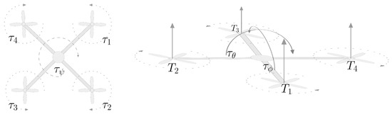
Figure 1.
Left-hand panel: Overhead view of a quadcopter, showing the rotors’ direction of rotation and resulting torques , as well as the resulting torque on the drone’s vertical axis. Right-hand panel: Side view of a quadcopter showing the thrusts generated by the rotors and the resulting torques and on the horizontal axes.
Each rotor i produces a vertical trust perpendicular to the quadcopter body. By controlling each rotor’s speed, it is possible to control the rotation of the drone along its horizontal axes (motions referred to as ‘pitching’ and ‘rolling’). As illustrated in Figure 1, to induce a rotation along one of these axes, it suffices to make one rotor spin faster (or slower) in such a way that the difference in thrust compared to the thrust generated by the opposite propeller yields a moment of force or that causes a rotation in the body. To avoid unwanted yawing, the increase in speed in one of the rotors must be compensated for by an equal decrease in the speed of the rotor opposite to it (along the same axis), which results in zero net torque along the body’s vertical axis.
3.1. Mathematical Model of a Quadcopter Drone
In the standard mathematical model [35], the dynamics of a quadcopter are described with the help of two frames of reference: the “earth” frame and the “body” frame. The dynamics of a quadcopter are described by its position vector in the earth frame and by its angular position (attitude) vector in the body frame:
where denotes the roll angle, namely, the rotation around the body-fixed frame x-axis, denotes the pitch angle, namely, the rotation around the body-fixed frame y-axis, while denotes the yaw angle, namely, the degree of rotation around the body-fixed frame z-axis.
In the body frame, the linear velocities and the angular velocities relative to the origin (the center of mass) are denoted as
To convert the angular velocities relative to the body frame into the attitude rate (the derivative with respect to time of the attitude ), a transformation matrix is introduced, whose inverse reads
where , and . The conversion rule between the two coordinate systems reads .
Since the rotors are able to generate thrust only along the z-axis of a quadcopter’s body, to obtain the resultant thrust vector relative to the earth frame of reference, it is necessary to make use of a rotation matrix that aligns the body frame to the inertial frame, defined as
A system-theoretic representation of a quadcopter’s dynamics takes as overall input the rotors’ speed vector , outputs the position and is described by an internal state attitude vector . The functional equations to describe the dynamics of a quadcopter are described as follows:
- From the current state (including the initial conditions), the torque and the thrust intensity T along the z-axis relative to the body frame are computed aswhere the constant l denotes the length of the drone’s arms, the constant k denotes the lift constant and the parameter b denotes the ‘drag’ constant of a single rotor. The above equations account for the spinning directions of the rotors as well as the efficiency of the rotors’ blades. The drag effect refers to the fact that the collective spinning of the rotors tends to make the body of the quadcopter spin as well along the vertical axis.
- On the basis of the torque vector , the angular acceleration of the quadcopter’s body relative to the body frame is calculated aswhere , and denote the moments of inertia of the quadcopter with respect to the principal axes of inertia, which are supposed to coincide to those of the reference frame, while denotes the moment of inertia of each rotor along the z-axis (which is the only inertia value of interest). Since the structure is—in good approximation—geometrically symmetrical, it is commonly assumed that . To compute the angular velocity vector in a computer-based implementation, the differential Equation (6) will be solved using numerical recipes.
- By using the transformation matrix , the attitude-change rate of the quadcopter relative to the ground can be obtained by a transformation of the angular velocity vector relative to the body frame :By numerically solving such a further differential equation, the attitude of the quadcopter is obtained at every time-step of the simulation.
- The center of mass’s acceleration relative to the earth frame is then obtained by applying the gravity acceleration directly and by applying the thrust force vector (divided by the drone’s mass and rotated using the attitude matrix ). The acceleration obeys Newton’s law:where m denotes the mass of the quadcopter, denotes the gravitational force (weight) directed towards the negative direction of the earth frame’s z-axis, namely, , where c denotes the gravitational acceleration constant and . In addition, the quantity denotes a friction matrix. Notice that since the force is only applied to the z-axis of the drone, only the third column of plays a role in such an equation. The relationship (8) may be cast in plain form aswhere and are the friction coefficients for the velocities in the x-, y- and z-direction, respectively, of the earth frame of reference.
3.2. Proposed Control Strategy
The main goal of this paper is the design of a controller to attain autonomous flight in a quadcopter system. The first step in the design was the definition of the drone’s desired behavior, followed by a planning of the appropriate control scheme and neural network training strategy.
The main goals of an autonomous flight controller are to make a quadcopter reach a fixed point in space, to keep it flying steadily over its trajectory and to keep it in the vicinity of a target. Defining the first objective is straightforward, while defining the second objective needs cautions and careful design, which might otherwise result in two conflicting goals. Such a problem might be fixed by means of multi-objective control and optimization techniques [36]. In particular, we invoked the notion of attitude limitation, which entails that a quadcopter has to tilt for as little time and angular extent as possible, and each rotation in one direction must be compensated for and countered by a rotation in the opposite direction. Such a design objective may be broken down into two parts: the first, regarding the spin time and amount, means that the desired final behavior is to obtain fast rotation (to comply with the optimality of trajectory) and to avoid states in which the drone tilts excessively; the second part, about the compensation of tilting along one direction, ensures that the quadcopter will eventually tilt in the opposite direction by an equal extent, thus attaining a horizontal attitude once the drone reaches the target. Such a notion does not cause any conflict: in order to reach the target, it may tilt as required by the optimal trajectory planning because there exist no constraints about the attitude angles, while, to reach the correct horizontal attitude, the second part of the stabilization requirements (namely, compensation of tilting) is prescribed. Furthermore, with the aim of avoiding extreme and unwanted tilting, which might cause a quadcopter to fall to the ground, a constraint on the maximum absolute values of the attitude pitch and roll angles is enforced. The mentioned set of requirements will be engraved into the cost-function definition, presented in Section 3.4.3, about the functioning of the evolutionary algorithms used to select and evolve a neurocontroller.
The above-sketched control mechanism will be extended to make a quadcopter follow a complex trajectory in space by subdividing a complex path in a series of sequential points and by providing a single target at a time, switching to the next one when the quadcopter is close enough to the current target.
3.3. Neural-Network-Type Controller Structure
The observable/measurable state used to control the quadcopter is obtained by stacking up the variables (coordinate of the center of mass), (linear velocity), (linear acceleration), (attitude angles), (body angular velocities). The reference input (set point) is the desired position of the quadcopter’s center of mass (target) . The control strategy is actuated using a feedback loop in which the current position is compared with the target, resulting in the position error . The state error is defined as:
The state error inputs the neural network controller, which outputs the appropriate motors’ angular speeds , the input to the quadcopter’s mathematical model. There are no reference inputs concerning the attitude of the drone. This allows the quadcopter to follow an optimal trajectory (not defined a priori) based on learning. Nevertheless, as a result of the aforementioned objectives’ definition and of the learning algorithm, once the quadcopter reaches the set point it will remain hovering in that position horizontally.
The controller’s neural network structure is a multilayer perceptron illustrated in Figure 2.
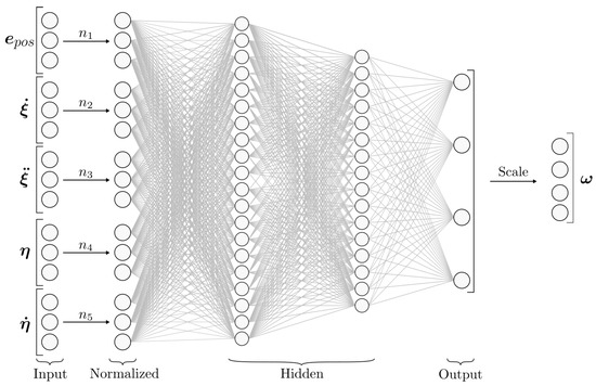
Figure 2.
Neural network structure including input and output signals. The topology shown is {15, 20, 6, 4}.
The network takes as input the state relative to the target , which is composed of five -vectors, for a total of 15 input nodes.
To improve the learning performance, the input elements are normalized to a range in the interval : each sub-vector of the error is normalized by the non-linear rule , where is the normalization factor of the corresponding input . This reduces the search space for the algorithm [37], thus improving its training performance by reducing and bounding the dimensionality of the problem from an input space to a space .
The normalized input then passes through h hidden layers, each of size , resulting in the output of the network . Each node is activated using a weighted and biased sigmoid , namely,
where denotes the nodes’ activation vector of the layer i, denotes the weight matrix from the current layer i to the next, of size , denotes the bias vector of layer i and represents the total number of layers (one input, one output and h hidden layers). The size of the vectors and are fixed at and , respectively, while the size and number of hidden layers may be varied. The values of the entries of and for , which determine the response of the controller to the current state, and the normalization scaling factors for are determined during the training stage by the learning algorithm.
The output of the network is a -vector. To obtain the rotors’ desired speeds, such a vector is mapped and scaled to the minimum and maximum rotors’ rotation speed (denoted as and , respectively) with the affine transformation:
3.4. Evolutionary Training Algorithm
In order to train the neural-network-based controller so that it complies with said control objectives, a learning algorithm along with a numerical simulation engine are engaged. In the present instance, the training process cannot be supervised, because the optimal trajectory is not predefined; hence, a training set (namely, the correct rotor speeds in response to specific states) is lacking. Even in the case of supervised learning, it appears that it would be extremely difficult and unpractical to obtain a sufficient amount of data to run, e.g., error back-propagation learning [38,39].
Therefore, an evolutionary learning strategy was the solution of choice. The implemented algorithm is of the evolutionary type. Compared to other algorithms in this family such as NEAT, the training algorithm does not modify the topology of the neural network; hence, the topology must be specified heuristically in advance. An overview of the devised algorithm is shown in Figure 3.
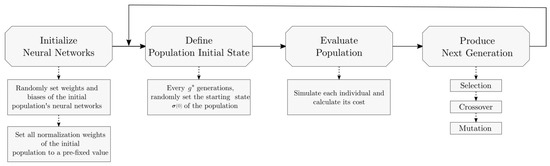
Figure 3.
Flow-chart of the evolutionary algorithm used to train a neural-network-based controller (see the following subsections for a detailed explanation).
The devised training algorithm is based on a population of individuals. At the beginning of every iteration, a new generation is created from the previous one. Any individual in the population, or agent, is defined as a single neural-controller, whose configuration is represented by a set of weights and biases.
The configuration of a neuro-controller, namely, the set of entries of its weight matrix and bias vector, is represented by a genome through a direct-encoding genotype representation [40]. The vector of coefficients of normalization is also added to the genotype. Direct encoding was preferred to other types of encoding because a more complex encoding was not needed since the training algorithm does not influence a network’s topology or embodies complex concepts such as speciation (namely, a subdivision of the population in specialized groups).
3.4.1. Initialization
At the start of the algorithm, the initial population of size p is created by assigning to each individual a a randomly generated genome.
The values of the connection weights and biases of a neurocontroller are initialized as follows:
where denotes a function that returns a real number drawn from a random distribution, bounded by a constant , namely .
The algorithm also operates on the normalizer weights; therefore, those parameters are also specified at the start as
where denotes a constant. In the first generation each individual possesses the same normalizer weights, but since the optimal value of is not known a priori, in the upcoming generations those weights will vary according to the evolution rules set forth. Such a mechanism allows the algorithm to also optimize the level of normalization that the input of the neural network undergoes, which can be interpreted as the neural network’s input sensitivity to each sub-vector of the input .
3.4.2. Starting State Definition
At the beginning of every generation, all the neurocontrollers in the population possess the same initial state . This means that every neurocontroller–quadcopter pair starts off from the same conditions; hence, despite the differences in each individual genome, each quadcopter is evaluated in the same exact way as the other individuals belonging to the same generation.
Furthermore, at each generation g, the starting state of each single controller is set. In the first generation, the initial state of each quadcopter is randomly set, namely,
where represents a random vector of the same size as x, with random entries bounded by a constant, namely, for . One such initialization carries over for as many as generations; after that, it is reset. For example, if , then , while is reset and then , and so forth.
Having an initial state that is not fixed, meaning that is very low compared to the total number of generations, is crucial to the functioning of the evolutionary training algorithm. The value of the integer is defined at the beginning of the training phase. In fact, if in every generation every individual were to start from the same state as the previous generation , without any variation, the neural networks would evolve to only exhibit the correct behavior for that fixed starting state, and when presented with a situation different from the one that they were evolved from, the neural networks would inevitably fail to control the quadcopter because of the lack of proper training. Instead, by varying the starting state very frequently, because of the evolutionary nature of the training algorithm, only the individuals that can effectively control the quadcopter in a multitude of different situations will transfer their genes to the next generation, resulting in each generation becoming better at handling different conditions.
To promote the exploration of the feasible state space, the boundary of the random state generation, represented by the constant , is set to higher values. For example, by increasing the value of the constant (the boundary for the random value of the elements in the attitude-rate sub-vector of the starting state ) and the constant (namely, the boundary of the initial velocity), the individuals will start a simulation with higher speeds in random directions and higher tilting speeds. This increases the harshness of the training and only the best individuals that can withstand those hard conditions will transfer their genes to the next generation. As a consequence, over several generations, the evolutionary algorithm will yield individuals that are able to handle such conditions, which corresponds to obtaining more robust and attitude-limitation-compliantneural controllers.
Notice, however, that if the values of the parameters are chosen too large, the starting conditions will be outright impossible to control; therefore, the evolution will not produce better individuals. In fact, in this instance, it would be impossible to evaluate and to distinguish the performance of poorly evolved individuals against the well-performing ones.
3.4.3. Population Evaluation
After the current generation’s starting state is defined, each individual (meant as a neurocontroller–quadcopter pair) is simulated using a discrete-time numerical simulation engine and its performance is evaluated. The generation index g ranges from 0 to a total number of generations G, which is fixed at the beginning of a training phase. The constant G determines the level of evolution of a neurocontroller.
Each individual a in the population is constrained by a fixed lifespan . Namely, from the instant to the last , its performance is evaluated. At each instant k, on the basis of the state , the individual a’s neural network outputs the rotor’s speed vector . Such a control vector is then used as input to the quadcopter mathematical model Q to calculate the next state of the individual quadcopter a over the set of p individuals belonging to the generation.
If an individual reaches a quota z of less then 0 m from the ground, for the purposes of the simulation such an individual is considered as crashed and its state will not be updated any longer, effectively remaining stuck in the position where it has collided with the ground. One such safety measure is necessary, otherwise quadcopters will not evolve to avoid crashing to the ground. In addition, such a mechanism speeds up the evaluation process because the crashed individuals need no further simulation efforts.
To evaluate the performance of the current generation, a cost function [40] that represents the inverse of the performance of an individual a (the higher the cost, the worse the individual’s performance) in the current generation is defined as follows:
where, relative to an individual a in the population , the cost component represents how poorly the controlled quadcopter reaches the target, the component represents how much its attitude has exceeded certain tilting thresholds, the component represents its noncompliance with the attitude-limitation requisite and the cost component embodies the information as to whether a quadcopter has ever crashed and, if it has, how long it had flown safely.
An individual should reach the target position in the shortest amount of time and stay in that position after reaching it. Such an aspect is evaluated and represented upon recording the displacement of the quadcopter relative to the target’s position:
where represents the time, in seconds, elapsed between step k and step (namely, the characteristic time-step of the chosen numerical-simulation engine).
As already underlined in Section 3.2, it is desirable that its attitude angles and do not exceed a certain threshold . In order to quantify compliance with the attitude-limitation constraints, a cost component related to the extent of tilting is defined as
where denotes a positive constant representing the penalty for exceeding the limit on the attitude angles. The ideal value ranges between rad and rad.
A further cost component to enforce attitude-limitation compliance, related to the speed of attitude variation, is defined as
In the quantity , the attitude-variation rates , and are compressed using a nonlinear function , then these values are accumulated along the life span of each individual. The compression of the attitude-variation rate is an important step: since the compression map is nonlinear, small rates of change in attitude maintained for longer periods of time result in a higher cost compared to fast changes in attitude happening over shorter periods of time.
The definition (19) needs a somewhat deeper discussion to justify its deployment. Since the components of the vector take the same sign as the components of , the sum of the values of over the life span of an individual is zero (the lowest cost possible) only if individual a tilts in such a manner so as to align with the correct trajectory and then, once it is about to reach the set point, starts to tilt in the opposite way compared to the previous tilting. In summary, this term promotes individuals that exhibit impulsive tilting behaviors and that compensate each rotation in one direction with one in the opposite direction.
Since it is desirable that the learned neurocontroller avoids crashing the quadcopter to the ground, a cost component is introduced to penalize crashing individuals as
where is a constant taking a large value, since the avoidance of crashing is a crucial requisite and the related cost component must stand predominantly when non-zero.
3.4.4. Next Population Generation with an Evolutionary Algorithm
The aim of an evolutionary algorithm is to yield a future generation that performs better than the previous one. The amount of time it takes to achieve an optimal solution is mainly determined by this phase. To achieve such a goal, for each individual a of the next generation , three steps are applied in sequence: (1) two individuals (parents) and are selected [41] from generation g (selection); (2) their genes are combined (crossover) to create offspring a; (3) the offspring undergoes a mutation process in its genome (mutation).
Not all p individuals evolve from one generation to the next; a number among the best individuals of the current generation will be transferred directly to the new generation. This is to avoid genetic drift, which can occur in two cases, namely, in the event that all the offspring of the new generation are heavily mutated, resulting in a worse performance, and in the event that the random starting state is too difficult to control, then the costs of the individuals in the mutated population would be similar to one another and not representative of the quality of an individual’s genome. An example of a difficult-to-control condition is when every individual starts off very close to the ground and upside down, and thus, most likely hitting the ground soon after the beginning of a simulation.
The three mentioned steps are detailed as follows:
Selection: For each individual a of the next generation , two parents and are selected from the population using a custom algorithm inspired by tournament selection [42]. To be more specific, a pool of individuals from population is formed by randomly choosing individuals to be candidate parents. Out of these, the two best individuals (namely, those with the lowest cost , ) are selected. The pool size is a fixed parameter to be carefully selected. In fact, a known problem of selection algorithms is ensuring a balance between exploration and exploitation [43]. Whenever the algorithm is focused on exploitation, it will become stuck in a local minimum, while if it only relies on exploration it will never settle on a minimum.
By increasing the pool size , the algorithm favors exploitation (if the maximum tournament size is the size of the population, the best two individuals will always be chosen) while, by lowering its size, exploration is favored (if the maximum tournament size equals two, the algorithm performs a completely random selection).
Crossover [44]: Once two parent individuals and are selected, to generate their offspring, a crossover between the genomes of and takes place. Since the genomes (weights, biases and normalization weights) are directly encoded, the chosen method for generating the genome of the offspring consists of picking each of its genes as one of its parental genes, with an equal chance between the two parents.
Mutation [45]: After an offspring a is obtained, it undergoes mutation with a non-deterministic function that determines whether this individual will mutate. The probability of mutation is expressed through a mutation rate . Mutation is realized adding a random number to one of its genes. Since the mutation algorithm modifies only one gene at a time, if the offspring a is mutated, the mutation function is called again to determine whether the individual will undergo mutation again. As a consequence, the mutation rate must be set relatively high () to increase the chance of an individual’s genetic heritage mutating in more than one gene.
Mutation in genetic algorithms is a fundamental step because, without it, the algorithm will only yield subsequent generations based on genes that are a combination of the first generation’s genes, resulting in a very limited exploration of the solution space. By adding a random number r, instead of directly assigning a random value, the mutation algorithm ensures that the genes are not strictly bounded to a pre-fixed interval. Moreover, better results in learning performance are obtained by setting the random number bound as a low value, because it makes the exploration strategy more graded. In fact, if the interval is too narrow, exploration, albeit more precise, is slower and more prone to becoming stuck in local minima of the criterion function .
The complete next-population-generation procedure is outlined in Algorithm 1.
| Algorithm 1 Next-population-generation algorithm |
|
4. Implementation
In this section, the programming techniques used to implement the evolutionary learning algorithm, as well as the neural control algorithm, are briefly summarized.
4.1. Numerical Implementation
The quadcopter model equations, which are expressed in the continuous-time domain, are converted to the discrete-time domain using the forward Euler method. Since the step size of the simulation has to be necessarily low (on the order of ) to ensure the neural network controller accesses timely information to control the quadcopter, the forward Euler method, albeit not the most precise of all the numerical procedures to approximate solutions to differential equations, was the method of choice. Moreover, in the present endeavor, performance was more important than absolute numerical precision, and the forward Euler method has proven to be a good compromise. Nevertheless, the quadcopter model discrete equations can be extended and solved using different methods without compromising the functioning of the program.
4.2. Software Implementation
The code was written in JAVA. Since the calculations involve matrices, the Efficient Java Matrix Library (EJML) was chosen, which is known to provide a very good performance, especially for dense small matrices such as those encountered in the present endeavor.
In order to be able to visually inspect the result of the developed code, a 3D virtual environment was implemented using Processing 3, a library that uses OpenGL® as a graphical engine and that can provide both 3D and 2D interactive visualizations. Furthermore, to add functionality to the software, as described below, a simple GUI using Swing was implemented. With the aim of decreasing the training computation times, the realized implementation of the evolutionary learning algorithm exploits multi-threading to simulate each individual in its life span.
The parameters of the quadcopter model, the neural network topology and the parameters of the evolutionary algorithm can be configured directly in a standalone JSON (JavaScript Object Notation) file, without the need to modify the source code.
4.2.1. Program Functionality
The main features of the developed software are:
- The program defines the simulation parameters in a configuration file;
- The code applies the evolutionary algorithm with the specified configuration, while a virtual 3D environment is showing the evolution of the generations;
- The program supplies the evolutionary algorithm without the 3D environment to increase the training speed;
- The software loads and saves the neural networks of a population produced by the algorithm in a JSON file;
- The program simulates (from a neural network file) and shows in 3D the best individual in that population while it runs along a randomly generated spatial path.
4.2.2. Exemplary Screenshots
For illustrative purposes, some screenshots of the virtual 3D environments are shown in what follows. Figure 4 displays a static view of the virtual 3D environment used for training, while Figure 5 shows the results of a 3D simulation of a single trained quadcopter running along a pre-defined path.
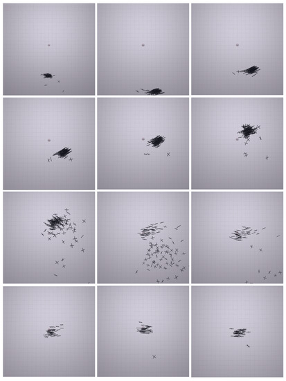
Figure 4.
Three-dimensional training environment of the evolutionary-type learning algorithm for a trained generation of p = 150 individuals. In each frame, the point in the center represents the target (set point) and the crosses represent each individual. From left to right and top to bottom, screenshots of the current generation’s quadcopters behaviors in time, each 0.1 s apart.
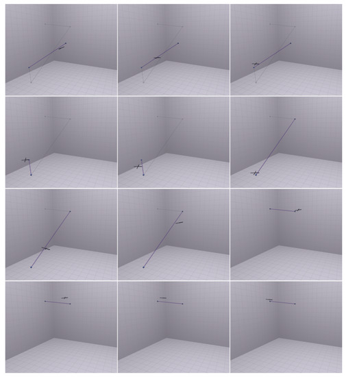
Figure 5.
Three-dimensional path-following environment. From left to right and top to bottom, the screenshots display the dynamics of a trained quadcopter’s behavior in time (each taken 0.6 s apart) while following a pre-defined path. The quadcopter is represented by a cross mark while the path, consisting of waypoints connected by short straight sub-paths, is represented by spheres and lines. Segments yet to be completed are drawn in light gray color, while the segment joining the previous target to the current target is highlighted in violet color.
The quadcopters shown in Figure 4 arose as the result of G = 20,000 generations trained over a “harsh configuration”, a condition described in detail in Section 5, to highlight the difference in the performances of individuals. In addition, the neurocontroller applied to the quadcopter whose dynamics are displayed in Figure 5 was trained over G = 250,000 generations over the same (harsh) configuration.
On the basis of Figure 4, the functioning of the evolutionary algorithm to yield a generation may be visually summarized. Initially, all individual controllers are given the same starting state , then such controllers start driving a quadcopter to reach the target point (represented as a sphere shown in the images’ center) and their performance is evaluated until the lifespan of the population is reached. As can be seen, a fraction of the individuals lose controland happen to fall to the ground. This is a normal behavior since the individual controllers have been trained over as little as G = 20,000 generations. Moreover, such behavior is a consequence of the random mutation process, which can improve or diminish the performance of certain individuals. Nevertheless, the better the performance of an individual, the higher the probability of transferring its genes to the next generation.
After training the neural networks over a desired amount of generations or time, the resulting controller’s performance can be qualitatively evaluated in the path-following environment shown in Figure 5. The software generates a path for the quadcopter to follow, displayed by a series of spheres connected by lines, and the quadcopter is supposed to visit each point sequentially. A quantitative evaluation of the quadcopter’s performance can be obtained by running the path-following tests programmatically, suppressing the on-screen animation outcomes, while outputting useful and meaningful data results to a file. This feature was used to collect the values shown in the figures and tables in Section 5.
5. Computer-Based Simulated Experiments
The present section illustrates the results of two types of experiments intended to assess the performance of the neural controller produced using the evolutionary learning algorithm and to discuss the results of neural network topology selection in training effectiveness and control outcome.
The values of the parameters used in the following numerical simulations, which take constant values irrespective of the simulation at hand, are summarized as:
- Parameters regarding the quadcopter model and its numerical simulation: , , , , , , , , , .
- Parameters of the evolutionary-type learning algorithm: , , , , , , , , , , , , , .
Each parameter value is expressed in International Systems units.
5.1. General Performance Assessment and Harshness Configuration Testing
The purpose of the tests presented in this section is to assess whether harsher training conditions yield more robust (less prone to crashing) and better-performing controllers for autonomous flight. In addition, the following tests demonstrate the performance of the controller in the task of following a trajectory, proving that—upon further refining—neural controllers are a viable alternative to other methods of control.
The harshness of the training is determined by the parameters , where x is a sub-vector of the state , which substantially determine how far the initial state of a quadcopter lies from the desired state. Higher values in these parameters mean that the quadcopter will explore harder states to control, while evolution is supposed to favor individuals that can adapt to such situations. Every configuration refers to the same parameter values summarized at the beginning of the present section, while the starting-state parameters are presented in Table 1.

Table 1.
Bounds for the randomly generated starting parameters in the harshness tests (in International Systems units). ‘Harsh’ stands for high level of harshness, ‘Medium’ stands for medium level of harshness, while ‘Soft’ stands for low level of harshness.
The topology of the neural network is the same for every configuration and was set to .
The test began by running the evolutionary algorithm for each configuration over G = 250,000 generations, yielding the trained population . As a benchmark for the algorithm performance, to run as many as 250,000 generations three times (one for each harshness configuration) takes 8 h on a dedicated server machine (2.30 GHz, 8 Intel® Nehalem class i7 cores, 16 GB RAM); hence, less than 3 h to complete training for a single configuration, on average.
From the last generation of each configuration, the best individual (the one with the lowest value of cost function) is chosen to participate in the path-following tests. In these tests, the three individuals are given the same series of 1000 randomly determined paths. Each path is composed of ten random points in a sequence (in addition to the origin of the trajectory) and each point has a maximum distance of 10 m from the previous point, to form a random spatial path of at most 100 m in length.
Since the controllers are trained to drive a drone only from a starting point to a waypoint at a time, once the quadcopter enters a spherical neighborhood of the current target point of radius , it switches to the next point in the sequence, thus covering the whole path. As will be shown in the following, the choice of the radius significantly influences the performance in the three configurations and determines the precision of a quadcopter’s trajectory.
After the three best neurocontrollers were selected (one for each level of harshness, namely ‘harsh’, ‘medium’ and ‘soft’), a number of tests was conducted that aimed at evaluating their performance by challenging the controlled quadcopters to follow randomly-generated paths of different complexity and by requiring different levels of precision.
5.1.1. Loose Path-Following
In these tests, the radius was set to 1 m, namely, as soon as a quadcopter is closer than one meter to the current target, it will start to chase the next waypoint in the sequence. A radius of 1 m makes the actual trajectory quite loose with respect to the desired trajectory; therefore, the precision in reaching the targets will be less favored compared to the average flight speed.
Exemplary results pertaining to a single randomly generated trajectory are discussed in the following for illustrative purpose. In addition, cumulative results will be presented concerning a large set of path-following tasks that allows the extraction of some statistical information from the numerous single tests with reference, in particular, to the traveling time to complete a task.
Figure 6 shows the trajectory of three quadcopters over one of the randomly generated paths.
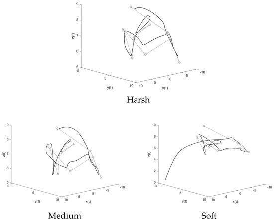
Figure 6.
Three-dimensional trajectories obtained in a loose ( = 1 m) path-following test. The dashed line denotes the reference path, while the solid line denotes the actual trajectory.
A first qualitative analysis can be carried out. The configuration learned from harsh conditions shows no problem in following the path and the resulting trajectory appears more steady than the others. The configuration trained from medium-harshness training conditions also completes the path, even though more jerky movements can be observed. The configuration trained on low-harshness conditions initially starts following the path but eventually crashes to the ground.
The trajectories followed by three quadcopters (each driven by one of the three selected controllers) can be observed with more detail in Figure 7, where the 3D path is projected along the three planes orthogonal to the coordinate axes.
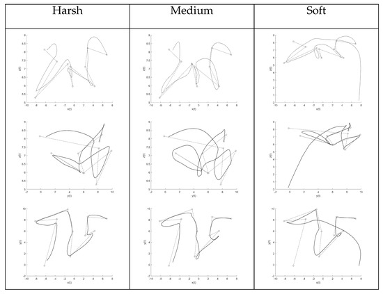
Figure 7.
Projections of the 3D paths of Figure 6. Upper row: Projection onto the x–z plane. Middle row: Projection onto the y–z plane. Lower row: Projection onto the x–y plane. (The dashed line denotes the reference path, while the solid line denotes the actual trajectory.)
From these graphs it can be observed that the quadcopters never quite reach the trajectory’s waypoints, because the value of the radius was set to a relatively large value. In addition, especially in the x–y plane (third row of graphs in the figure), the difference in the three trajectories is more marked.
As a safety note to correctly interpret the graphical results, let us recall that in Figure 6 and Figure 7 the dashed trajectories are just the connection between successive target points and do not constitute a reference input for the quadcopter. Moreover, the dashed trajectory is not always guaranteed to be the optimal trajectory for a quadcopter to follow.
The harsh training configuration drives the quadcopter through smooth movements with less pronounced bumps, and its trajectory follows more closely the straight path between the points. The medium training configuration yields a more erratic trajectory compared to the harsh configuration, but nevertheless completes the path-following task.
The soft training configuration initially closely follows the path. A noteworthy outcome is that, on the x–y plane, the soft training configuration even follows the path better than the harsh training configuration, which was expected to perform better than the other two configurations. Then, once it reaches a condition that it has not evolved to endure, the quadcopter crashes into the ground.
Again with reference to the single path-following test discussed via the Figure 6 and Figure 7, it is instructive to check the course of the norm of the positional error over time, as illustrated in Figure 8.
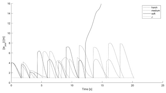
Figure 8.
Norm of the position error over time resulting from the three training configurations (harsh, medium, soft), in the loose ( = 1 m) path-following test.
From this figure it is immediate to see how the positional error is lower-bounded by the safety radius . Moreover, in this specific test, the positional error keeps bound along the whole trajectory in the harsh and the medium configuration, while it diverges for the soft controller. Such behavior reflects the results shown, e.g., in Figure 6, where it can be clearly witnessed as eventually the controlled quadcopter crashes to the ground.
Since every controller of each configuration has to traverse the same 1000 paths, the time each quadcopter takes to traverse a path can be used as a reference for its performance. The average travel time was determined by averaging these 1000 travel intervals. In addition, the minimum and maximum travel times were recorded.
Notice that, in general, not every quadcopter reaches the end of each path, since either a quadcopter crashes into the ground or it eventually keeps hovering mid-way without ever entering the safety bubble around a target that will trigger the next target (such a disruptive event is referred to as a stall).
In the loose path-following tests, incomplete trajectories only resulted from crashing (none from stalling), since the spherical neighborhood was chosen to be relatively wide. (The steady-state positional error should have been larger than 1 m if a quadcopter was to reach a stall situation, which turned out not to be the case with the chosen target-switch threshold ).
The numerical results for the traveling times are reported in Table 2.
Table 2.
Summary of 1000 loose ( = 1 m) path-following tests in terms of traveling intervals and number of disruptive events.
The harshly-trained quadcopter controller appears to be the most attitude-limitation-compliantof the three: over 1000 paths traversed, it never caused crashes or stalls once. However, as a counterpoint to the attitude-limitation compliance, the controlled quadcopter flight appears to be slower than the quadcopter evolved with softer starting states. The softly-trained configuration performs the fastest, with an average time of 17.59 s to run across 100 m, which corresponds to an average speed of 20.47 km per hour. The medium training configuration figures do not stand in between the harshly-trained and the softly-trained, exhibiting much more crashes and slower flight compared to the other configurations.
On the basis of the above results, we concluded that:
- The harsh training produces more stable and more ‘careful’ controllers that are not prone to make a quadcopter crash, at the cost of some slowdown along the trajectory.
- The soft training yields faster and more ‘reckless’ individuals, at the cost of occasional crashes where the quadcopter visits a state that it was not evolved to cope with.
- The medium-harshness training causes deplorable effects compared to the harsh and the soft training in terms of speed and reliability. Such a result is due to the fact that the training conditions are not harsh enough to produce reliable individuals, yet they are harsh enough to hinder the training process in evolving fast individuals.
The gathered numerical-experimental data show that with harsh training conditions, the evolutionary algorithm produces neural controllers that are both reliable and well-performing in the task of loose path-following autonomous flight.
5.1.2. Tight Path-Following
In order to gain a deeper insight about the features of the devised neurocontroller training method, further tests were run by setting the target-switch threshold to be equal to 0.1 m. Such a choice implies that the evolutionary neurocontrollers will have to steer a quadcopter to ensure it reaches the current target more tightly to trigger the next waypoint.
To this aim, and to make sure a quadcopter is effectively able to seamlessly reach the end of each path, attitude-limitation compliance in control is a tight requirement to avoid crashing into the ground, and a low steady-state error is also compulsory to avoid stalling in midair. In contrast to the tests described in Section 5.1.1, precision in reaching the target points is to be favored over travel speed; hence, longer travel times were expected.
As can be seen in Figure 9, the quadcopter’s controller trained under harsh training conditions is more than capable of following the prescribed trajectory with enough precision (relative to the target points), while the quadcopters’ controllers trained under medium and soft training configurations fail to reach the end of the path because they stall, hovering around one point, without reaching a distance less than to the current target and, hence, never advancing towards the end of the sequence.
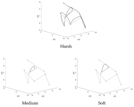
Figure 9.
Three-dimensional trajectories for the tight ( = 0.1 m) path-following tests. The dashed line denotes the reference path, while the solid line denotes the actual trajectory.
For the sake of better clarity, in this tight path-following test, the actual trajectories followed by three quadcopters whose neurocontrollers were each trained under harsh, medium and soft conditions were represented through projections on the planes perpendicular to the three axes, as shown in Figure 10.
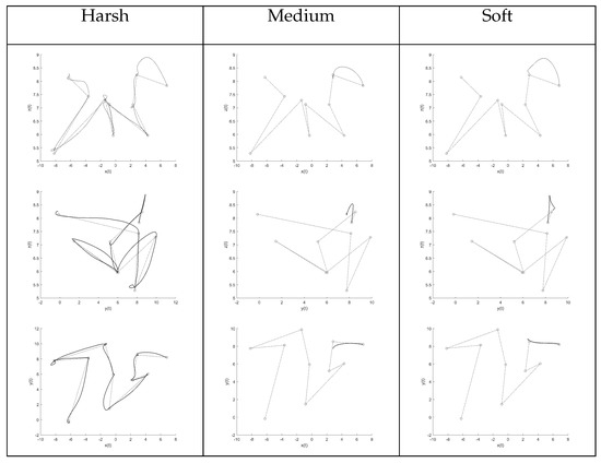
Figure 10.
Projections of the 3D paths of Figure 9. Upper row: Projection over the x–z plane. Middle row: Projection over the y–z plane. Lower row: Projection over the x–y plane. (The dashed line denotes the reference path, while the solid line denotes the actual trajectory.)
It is immediate to recognize that, in this particular path taken as an example, the controller is not always able to drive a quadcopter along a whole trajectory. In fact, both controllers trained under medium and a soft training conditions fail to properly direct the quadcopter.
The above result confirms that the softness of the training conditions is a primary cause of a lack of ability of a neurocontroller: the harder the conditions of training, the better the resulting control performances. In contrast, soft training conditions make a neurocontrolled quadcopter more prone to crashing into the ground and to stalling in mid-air. It is certainly beneficial to investigate the causes of such disruptive events more closely.
By observing Figure 11, the phenomenon of stalling, in particular, can be inspected more closely. Let us recall that a steady decrease in the positional error indicates that a controlled quadcopter is becoming closer and closer to the current target waypoint. In addition, a spike in the error curve means that the individual reached the spherical neighborhood of radius m and was henceforth triggered to started chasing the next waypoint in the sequence.
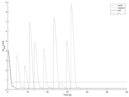
Figure 11.
Norm of the error of position of the three configurations in the tight ( = 0.1 m) path-following test versus time.
The error curve corresponding to the harsh configuration exhibits a sequence of nine spikes, which indicate that all of the ten waypoints in the path have been visited. The medium-trained and soft-trained individuals start chasing the first target point, but never reach an error less than ; thus, these neurocontrolled quadcopters keep hovering around the first waypoint without visiting any further locations in the path sequence. As a matter of fact, the medium-trained neurocontrolled quadcopter exhibits a steady-state error of about 0.8 m, while the soft-trained quadcopter shows a steady-state error of about 0.12 m, while the threshold that triggers the next waypoint was fixed to 0.1 m.
The travel times and number of incomplete paths (due to disruptive events recognized as stalls and crashes) are presented in Table 3.
Table 3.
Result summary of 1000 independent tight ( = 0.1 m) path-following tests (times expressed in seconds).
By comparing these results with those in Table 2, the difference in the three configurations appears more evident. The quadcopters controllers trained through a harsh configuration showed no issues in completing both the loose path-following task (with m) and the tight path-following task (with = 0.1 m), albeit showing an increase in travel times to complete the tight path-following task. In contrast, the neural controllers yielded by the medium and soft training configurations did not achieve a sufficiently low steady-state error to even complete one path out of one thousand.
5.1.3. Additional Precision Tests
Since the medium and soft training configurations have been proven inadequate, to further test the precision of the neural controller learned by the harsh training configuration, a number of additional tests was conducted. To evaluate the performance of the harsh training configuration, a series of trials, each conducted over a set of 10,000 randomly generated paths corresponding to different settings, was realized. The aim of these tests was to define the boundary of the test conditions within which the harsh training may still yield a successful controller.
The obtained results are summarized in Table 4.
Table 4.
Results obtained with a harsh training configuration over 7 kinds of experiments, each conducted on a set of 10,000 randomly generated paths corresponding to different values of the path parameters ℓ and (as explained in the text). The times are expressed in seconds while distances are expressed in meters.
Each row of the table pertains to the results of 10,000 randomly generated paths corresponding to specific values of two parameters: ℓ represents the number of points in a path and denotes the maximum distance between consecutive points of the paths (in meters). The parameter denotes the safety radius that triggers the next chased target in a path sequence. The results summarized in Table 4 indicate that for values of less than m the controller’s steady-state positional error is larger than the required threshold to advance the sequence of points in the path. This observation gives an approximate indication that the steady-state error is not larger than 0.085 m.
The neural controller trained and selected through the evolutionary algorithm with the harsh training configuration reached adequate levels of precision, with an average steady-state error of about 8 cm. It also ensures adherence to attitude-limitation constraints, with no crashes over the course of all tests.
5.2. Experiments on Different Network Topologies
The purpose of the following tests is to evaluate the effect that a network’s topology has on the performance of a neurocontroller in terms of learning ability. Three configurations of a neurocontroller were chosen that differ from one another only in the number of layers and number of neurons per layer. These topologies were selected to be:
- Complex topology: (which will be referred to as ‘complex’),
- Medium-size topology: (which will be referred to as ‘medium’),
- Simple topology: (which will be referred to as ‘simple’).
In order to train each neural network with the evolutionary learning algorithm, as many as G = 200,000 generations with as many as p = 100 individuals each were used.
On the basis of these parameters values, the evolutionary-type learning algorithm insists on less-trained individuals than the parameters chosen in the tests discussed in Section 5.1 (namely, 50,000 generations and 50 individuals less than the previous harshness tests). Such a pair was in fact chosen so as to highlight the effects of neural network topology on training times, disregarding the goal of producing fully trained individuals. Moreover, the primary objective of these tests was to qualitatively evaluate the effect that topology has on the training algorithm, although some path-following tests were also performed to obtain an approximate evaluation of the performance of the evolved individuals, albeit not fully trained.
To gather information on the training process, in each configuration’s generation the minimum cost of the entire population was recorded. Since the starting state resets every generations, the costs exhibit large fluctuations. Notice that the starting states are randomly determined, and the starting states that each configuration’s training session endures are independent of the starting states of the other two configurations.
Therefore, in order to increase the readability and interpretability of the results illustrated in Figure 12, the values to report in the plots were chosen to be the moving average (MA) of each generation’s minimum costs, calculated within a window of 2000 generations.
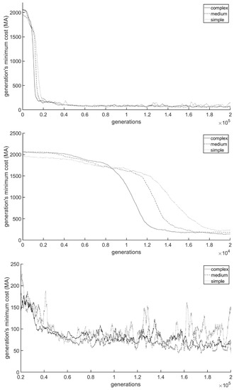
Figure 12.
Moving average of each generation’s minimum costs of each topological configuration within a window of 2000 generations. The curves represent, from the top panel to the bottom panel, the values for the entire training (G = 200,000 generations), the values at the start of the training (from generation g = 0 to g = 20,000) and the values in the remaining generations (from g = 20,001 to g = 200,000).
The curves in this figure show that initially the simple topology learns the quickest (lowest decreasing cost over each generation), the complex learns the slowest and the medium-topology training performance stands in between. After the initial learning phase, the simple topology exhibits, on average, the highest costs, while the medium and complex configurations exhibit lower costs. It is hard to determine the best topology between the medium and complex ones.
In order to assess the performance of the trained controllers, each controller was evaluated on a series of path-following tests, each totaling 500 paths with different numbers of waypoints and different maximal distances between two consecutive waypoints. This comparison was conducted in terms of the minimal, maximal and average traveling times for each category of paths. The obtained results are shown in Table 5.
Table 5.
Results of a series of tests, each totaling 500 randomly generated paths corresponding to different configurations, run on the final best controllers learned by means of the evolutionary algorithm for each of the three topologies (times expressed in seconds and distances expressed in meters).
The obtained results show that in loose path-following ( = 1 m) the neural network with the medium-complexity topology performs better, in terms of both travel time and attitude-limitation compliance, than the two competing instances of topology. The neural network with the simplest topology cannot complete a single test without crashing or stalling. The most complex topology in the loose path-following test performs adequately, but in the tests where the quadcopter must get closer to the path’s target waypoints ( = 0.5 m and = 0.1 m), the controller did not perform well enough to complete the paths reliably.
Such observations suggest that the topology of a neural controller must be chosen carefully. A complex topology (in both depth and width) requires more training time and does not necessarily entail an optimal performance. In contrast, a simpler topology requires less training time but does not possess enough capabilities for learning more complex tasks nor for learning the correct behavior corresponding to the states visited during training. Therefore, a good balance between the training speed and learning potential must be established by specifying a correct neural network topology.
6. Conclusions
The present research work assessed, through virtual experiments, the suitability of evolutionary neural networks in controlling quadcopter systems. Furthermore, the potentialities of an evolutionary algorithm as a method for a neural network’s unsupervised learning (neuro-evolutionary algorithms) were shown. It appears that, by defining an appropriate cost function to describe the control task and by tweaking the algorithm’s parameters, evolutionary techniques are able to train well-performing neural networks in a relatively short amount of time. The devised learning algorithm made the neural controllers perform the task of autonomous flight while upholding attitude limitations in a simulated environment with no obstacles.
To further extend the present work and make the analyzed control strategy more viable in real-world applications, the quadcopter can be equipped with an array of sensors for collision avoidance and its structure and learning processes modified to take into account supplementary inputs, such as visual data [38]. Moreover, the training environment can be ameliorated by adding disturbances such as wind or sensor noise to further improve the robustness of the controllers. The applications of this form of controller and training can also be extended to a vast amount of necessities. For example, to adapt the controller to logistic purposes (such as autonomous package delivery), the simulation can be expanded by adding a variable payload to the quadcopter so that the neuro-evolutionary algorithm can generate neural networks capable of adapting to deliver any type of reasonable cargo.
As noticed by a reviewer, the input to the neural network is the system state error normalized with a squashing function, while the system output rotor speed is transformed with a linear affine transformation. In this case, it could be the case that the rotor speed changes abruptly whenever the position error lies within the saturation branch of the squashing function. Moreover, on the basis of the experimental trajectory-tracking results, it was noticed that the closer to the target points, the slower the speed results. Although it is possible to operate in this way between two target points, all points are linked as one trajectory and the curvature factor would need to be taken into account as a subject of future research.
When performing the cost-function design, it is of practical significance to remove crashed quadcopters. The research endeavor could be pushed further by considering the case of the flight speed exceeding the intrinsic limit of the rotor speed. In fact, the physical realizability of the neurocontroller’s demand is a crucial aspect that was not taken into account while conducting the present research endeavor and that could be a subject of future research efforts.
The second author and a coworker have recently developed a specific PID-type control strategy [46] that may be taken as a starting point for a comparison of standard PID control and evolutionary-strategy-based control.
Author Contributions
Conceptualization, M.M. and S.F.; software, M.M.; writing—original draft preparation, M.M. and S.F.; writing—review and editing, S.F.; supervision, S.F. All authors have read and agreed to the published version of the manuscript.
Funding
This research received no external funding. The present paper summarizes the results of an autonomous project conducted and ended in 2020.
Data Availability Statement
The values of the parameters used in the numerical experiments are reported within the manuscript. The data to achieve training were generated randomly by the computer code itself.
Acknowledgments
The authors acknowledge the Dipartimento di Ingegneria dell’Informazione (UnivPM) for providing an advanced computation facility to conduct the numerical simulations. A copy of the Java code may be requested to the first author by email.
Conflicts of Interest
The authors declare no conflict of interest.
References
- Barbedo, J. A review on the use of unmanned aerial vehicles and imaging sensors for monitoring and assessing plant stresses. Drones 2019, 3, 40. [Google Scholar] [CrossRef]
- Budiharto, W.; Chowanda, A.; Gunawan, A.; Irwansyah, E.; Suroso, J. A Review and Progress of Research on Autonomous Drone in Agriculture, Delivering Items and Geographical Information Systems (GIS). In Proceedings of the 2019 2nd World Symposium on Communication Engineering (WSCE), Nagoya, Japan, 20–23 December 2019; pp. 205–209. [Google Scholar]
- Hassanalian, M.; Rice, D.; Abdelkefi, A. Evolution of space drones for planetary exploration: A review. Prog. Aerosp. Sci. 2018, 97, 61–105. [Google Scholar] [CrossRef]
- Lee, S.; Choi, Y. Reviews of unmanned aerial vehicle (drone) technology trends and its applications in the mining industry. Geosystem Eng. 2016, 19, 197–204. [Google Scholar] [CrossRef]
- Rao Mogili, U.; Deepak, B. Review on application of drone systems in precision agriculture. Procedia Comput. Sci. 2018, 133, 502–509. [Google Scholar] [CrossRef]
- Morris, K.C.; Schlenoff, C.; Srinivasan, V. Guest Editorial: A remarkable resurgence of artificial intelligence and its impact on automation and autonomy. IEEE Trans. Autom. Sci. Eng. 2017, 14, 407–409. [Google Scholar] [CrossRef]
- Erginer, B.; Altug, E. Modeling and PD control of a quadrotor VTOL vehicle. In Proceedings of the 2007 IEEE Intelligent Vehicles Symposium, Istanbul, Turkey, 13–15 June 2007; pp. 894–899. [Google Scholar]
- Bolandi, H.; Rezaei, M.; Mohsenipour, R.; Nemati, H.; Smailzadeh, S. Attitude control of a quadrotor with optimized PID controller. Intell. Control. Autom. 2013, 4, 335–342. [Google Scholar] [CrossRef]
- Li, J.; Li, Y. Dynamic analysis and PID control for a quadrotor. In Proceedings of the 2011 IEEE International Conference on Mechatronics and Automation, Beijing, China, 7–10 August 2011; pp. 573–578. [Google Scholar]
- Salih, A.L.; Moghavvemi, M.; Mohamed, H.A.F.; Gaeid, K.S. Modelling and PID controller design for a quadrotor unmanned air vehicle. In Proceedings of the 2010 IEEE International Conference on Automation, Quality and Testing, Robotics (AQTR), Cluj-Napoca, Romania, 28–30 May 2010; Volume 1, pp. 1–5. [Google Scholar]
- Szafranski, G.; Czyba, R. Different approaches of PID control UAV type quadrotor. In Proceedings of the International Micro Air Vehicles Conference 2011 Summer Edition, ’t Harde, The Netherlands, 12–15 September 2011; pp. 70–75. [Google Scholar] [CrossRef]
- Saif, A.W.; Dhaifullah, M.; Al-Malki, M.; El Shafie, M. Modified backstepping control of quadrotor. In Proceedings of the International Multi-Conference on Systems, Signals & Devices, Chemnitz, Germany, 20–23 March 2012; pp. 1–6. [Google Scholar]
- Argentim, L.M.; Rezende, W.C.; Santos, P.E.; Aguiar, R.A. PID, LQR and LQR-PID on a quadcopter platform. In Proceedings of the 2013 International Conference on Informatics, Electronics and Vision (ICIEV), Dhaka, Bangladesh, 17–18 May 2013; pp. 1–6. [Google Scholar]
- Besnard, L.; Shtessel, Y.; Landrum, B. Quadrotor vehicle control via sliding mode controller driven by sliding mode disturbance observer. J. Frankl. Inst. 2012, 349, 658–684. [Google Scholar] [CrossRef]
- Siti, I.; Mjahed, M.; Ayad, H.; El Kari, A. New trajectory tracking approach for a quadcopter using genetic algorithm and reference model methods. Appl. Sci. 2019, 9, 1780. [Google Scholar] [CrossRef]
- Grzonka, S.; Grisetti, G.; Burgard, W. A fully autonomous indoor quadrotor. IEEE Trans. Robot. 2011, 28, 90–100. [Google Scholar] [CrossRef]
- Rodić, A.; Mester, G.; Stojković, I. Qualitative evaluation of flight controller performances for autonomous quadrotors. In Intelligent Systems: Models and Applications; Springer: Berlin/Heidelberg, Germany, 2013; pp. 115–134. [Google Scholar]
- Leal, I.S.; Abeykoon, C.; Perera, Y.S. Design, Simulation, Analysis and Optimization of PID and Fuzzy Based Control Systems for a Quadcopter. Electronics 2021, 10, 2218. [Google Scholar] [CrossRef]
- Pham, T.; Ichalal, D.; Mammar, S. LPV and nonlinear-based control of an autonomous quadcopter under variations of mass and moment of inertia. IFAC-PapersOnLine 2019, 52, 176–183. [Google Scholar] [CrossRef]
- Bai, Y.; Gururajan, S. Evaluation of a Baseline Controller for Autonomous “Figure-8” Flights of a Morphing Geometry Quadcopter: Flight Performance. Drones 2019, 3, 70. [Google Scholar] [CrossRef]
- Bakar, A.; Ke, L.; Liu, H.; Xu, Z.; Wen, D. Design of low altitude long endurance solar-powered UAV using genetic algorithm. Aerospace 2021, 8, 228. [Google Scholar] [CrossRef]
- Kaufmann, E.; Loquercio, A.; Ranftl, R.; Dosovitskiy, A.; Koltun, V.; Scaramuzza, D. Deep drone racing: Learning agile flight in dynamic environments. In Proceedings of the 2nd Annual Conference on Robot Learning, CoRL 2018, Zürich, Switzerland, 29–31 October 2018; Volume 87, pp. 133–145. [Google Scholar]
- Lambert, N.; Drew, D.; Yaconelli, J.; Levine, S.; Calandra, R.; Pister, K. Low-level control of a quadrotor with deep model-based reinforcement learning. IEEE Robot. Autom. Lett. 2019, 4, 4224–4230. [Google Scholar] [CrossRef]
- Dierks, T.; Jagannathan, S. Neural network control of quadrotor UAV formations. In Proceedings of the 2009 American Control Conference, St. Louis, MO, USA, 10–12 June 2009; pp. 2990–2996. [Google Scholar]
- Pham, H.; Soriano, T.; Ngo, V.; Gies, V. Distributed adaptive neural network control applied to a formation tracking of a group of low-cost underwater drones in hazardous environments. Appl. Sci. 2020, 10, 1732. [Google Scholar] [CrossRef]
- Loquercio, A.; Kaufmann, E.; Ranft, R.; Müller, M.; Koltun, V.; Scaramuzza, D. Learning high-speed flight in the wild. Sci. Robot. 2021, 6. [Google Scholar] [CrossRef] [PubMed]
- Perez, R.; Arnal, J.; Jansen, P. Neuro-evolutionary control for optimal dynamic soaring. In Proceedings of the AIAA Scitech 2020 Forum, Orlando, FL, USA, 6–10 January 2020. [Google Scholar] [CrossRef]
- Stanley, K.; Miikkulainen, R. Evolving Neural Networks through Augmenting Topologies. Evol. Comput. 2002, 10, 99–127. [Google Scholar] [CrossRef]
- Shepherd, J.; Tumer, K. Robust neuro-control for a micro quadrotor. In Proceedings of the 12th Annual Conference on Genetic and Evolutionary Computation, GECCO’10, New York, NY, USA, 7–10 July 2010; pp. 1131–1138. [Google Scholar] [CrossRef]
- Alhmoud, L.; Al Dairy, A.R.; Faris, H.; Aljarah, I. Prediction of Hysteresis Loop of Barium Hexaferrite Nanoparticles Based on Neuroevolutionary Models. Symmetry 2021, 13, 1079. [Google Scholar] [CrossRef]
- Xu, J.; Chen, J.; Chen, S. Efficient Opponent Exploitation in No-Limit Texas Hold’em Poker: A Neuroevolutionary Method Combined with Reinforcement Learning. Electronics 2021, 10, 2087. [Google Scholar] [CrossRef]
- Ullah, Q.Z.; Khan, G.M.; Hassan, S.; Iqbal, A.; Ullah, F.; Kwak, K.S. A Cartesian Genetic Programming Based Parallel Neuroevolutionary Model for Cloud Server’s CPU Usage Prediction. Electronics 2021, 10, 67. [Google Scholar] [CrossRef]
- Giernacki, W. Minimum energy control of quadrotor UAV: Synthesis and performance analysis of control system with neurobiologically inspired intelligent controller (BELBIC). Energies 2022, 15, 7566. [Google Scholar] [CrossRef]
- Mendívez Vásquez, B.L.; Barca, J.C. Adversarial scenarios for herding UAVs and counter-swarm techniques. Robotica 2023, 41, 1436–1451. [Google Scholar] [CrossRef]
- Luukkonen, T. Modelling and Control of Quadcopter. Independent Research Project in Applied Mathematics, Aalto University, School of Science, 2011. Available online: https://sal.aalto.fi/publications/pdf-files/eluu11_public.pdf (accessed on 11 October 2018).
- Gambier, A.; Badreddin, E. Multi-objective optimal control: An overview. In Proceedings of the 2007 IEEE International Conference on Control Applications, Singapore, 1–3 October 2007; pp. 170–175. [Google Scholar] [CrossRef]
- Srinivas, M.; Patnaik, L. Learning neural network weights using genetic algorithms-improving performance by search-space reduction. In Proceedings of the 1991 IEEE International Joint Conference on Neural Networks, Singapore, 18–21 November 1991; Volume 3, pp. 2331–2336. [Google Scholar]
- Xue, Z.; Gonsalves, T. Vision based drone obstacle avoidance by deep reinforcement learning. AI 2021, 2, 366–380. [Google Scholar] [CrossRef]
- Chithapuram, C.; Jeppu, Y.; Kumar, C.A. Artificial Intelligence guidance for Unmanned Aerial Vehicles in three dimensional space. In Proceedings of the 2014 International Conference on Contemporary Computing and Informatics (IC3I), Mysore, India, 27–29 November 2014; pp. 1256–1261. [Google Scholar] [CrossRef]
- Whitley, D. A genetic algorithm tutorial. Stat. Comput. 1994, 4, 65–85. [Google Scholar] [CrossRef]
- Bäck, T.; Hoffmeister, F. Extended selection mechanisms in genetic algorithms. In Proceedings of the 4th International Conference on Genetic Algorithms, San Diego, CA, USA, 13–16 July 1991; Morgan Kaufmann: Burlington, MA, USA, 1991; pp. 92–99. [Google Scholar]
- Miller, B.; Goldberg, D. Genetic algorithms, tournament selection, and the effects of noise. Complex Syst. 1995, 9, 193–212. [Google Scholar]
- Črepinšek, M.; Liu, S.H.; Mernik, M. Exploration and exploitation in evolutionary algorithms: A survey. ACM Comput. Surv. 2013, 45. [Google Scholar] [CrossRef]
- Poon, P.; Carter, J. Genetic algorithm crossover operators for ordering applications. Comput. Oper. Res. 1995, 22, 135–147. [Google Scholar] [CrossRef]
- Bäck, T. Optimal mutation rates in genetic search. In Proceedings of the Fifth International Conference on Genetic Algorithms, San Francisco, CA, USA, 1 June 1993. [Google Scholar]
- Fiori, S.; Bigelli, L.; Polenta, F. Lie-group type quadcopter control design by dynamics replacement and the virtual attractive-repulsive potentials theory. Mathematics 2022, 10, 1104. [Google Scholar] [CrossRef]
Disclaimer/Publisher’s Note: The statements, opinions and data contained in all publications are solely those of the individual author(s) and contributor(s) and not of MDPI and/or the editor(s). MDPI and/or the editor(s) disclaim responsibility for any injury to people or property resulting from any ideas, methods, instructions or products referred to in the content. |
© 2023 by the authors. Licensee MDPI, Basel, Switzerland. This article is an open access article distributed under the terms and conditions of the Creative Commons Attribution (CC BY) license (https://creativecommons.org/licenses/by/4.0/).