Abstract
The current research into decision-making strategies for air combat focuses on the performance of algorithms, while the selection of actions is often ignored, and the actions are often fixed in amplitude and limited in number in order to improve the convergence efficiency, making the strategy unable to give full play to the maneuverability of the aircraft. In this paper, a decision-making strategy for close-range air combat based on reinforcement learning with variable-scale actions is proposed; the actions are the variable-scale virtual pursuit angles and speeds. Firstly, a trajectory prediction method consisting of a real-time prediction, correction, and judgment of errors is proposed. The back propagation (BP) neural network and the long and short term memory (LSTM) neural network are used as base prediction network and correction prediction network, respectively. Secondly, the past, current, and future positions of the target aircraft are used as virtual pursuit points, and they are converted into virtual pursuit angles as the track angle commands using angle guidance law. Then, the proximity policy optimization (PPO) algorithm is applied to train the agent. The simulation results show that the attacking aircraft that uses the strategy proposed in this paper has a higher win rate during air combat and the attacking aircraft’s maneuverability is fully utilized.
1. Introduction
With the development of unmanned aerial vehicles (UAVs) technology and stealth technology, the importance of close-range air combat has increased again and cannot be ignored [1]. The strategy and algorithm of decision-making directly affect the results of close-range air combat and have been extensively studied.
At present, traditional decision-making methods in air combat mainly include game theory, optimization, method expert system, and so on [2]. The methods based on game theory include differential games and image graph games. In Ref. [3], a decision-making strategy based on differential game was proposed for UAVs in close-range air combat. In Ref. [4], the multi-level influence graph was applied to solve the decision-making problem of multi-aircraft cooperative combat. The method based on optimization theory transforms the air combat problem into a multi-objective optimization problem using approximate dynamic programming (ADP) [5], genetic algorithm (GA) [6], particle swarm optimization (PSO) [7], Bayesian programming [8], etc., which were all applied to solve the problem. The core of the decision-making method based on expert systems is to propose a rule base and generate commands according to past experiences in air combat. Adaptive maneuvering logic (AML) [9] was developed by NASA for one-to-one air combat. In Ref. [10], a strategy based on pilot experience and tactical theory was proposed for autonomous decision-making in air combat. However, due to the continuity and complexity of the air combat state space, decision-making strategies based on traditional methods are often only suitable for offline planning and have poor real-time performance.
With the development of artificial intelligence, machine learning has become a hot topic in air combat decision-making strategies. The reinforcement learning method transforms the problem into a sequential decision-making problem and conducts self-play through continuous interactions with the air combat environment. The actions and rewards are combined, and long-term rewards are considered, which has certain advantages in solving complex air combat problems. The algorithms of the deep q network (DQN) [11], deep deterministic policy gradient (DDPG) [12], and twin delayed deep deterministic policy gradient (TD3) [13] have been applied to make decisions in air combat. In addition, multi-agent reinforcement learning algorithms such as multi-agent deep deterministic policy gradient (MADDPG) [14] and multi-agent hierarchical policy gradient (MAHPG) [15] have been widely discussed.
However, in the present research, the performance of algorithms is widely discussed, but the selection of actions is often ignored. Regardless of discrete or continuous action, the amplitude of action is usually fixed, and the number of actions is limited to improve convergence efficiency, such as the 7 extreme actions proposed by NASA [16] or the 27 maneuvering actions using command change rate [17]. The effect of the strategy is constrained by the actions, and the maneuverability of the aircraft may not be fully utilized.
In this paper, a decision-making strategy for close-range air combat based on reinforcement learning with variable-scale actions is proposed. The actions are not commonly fixed-amplitude commands but variable-scale virtual pursuit angles and speeds. Firstly, the model of close-range air combat is established, and the differences between the strategy with variable-scale actions proposed in this paper, the traditional reinforcement learning method, and the traditional virtual pursuit points (VPPs) guidance law are compared. Then, the trajectory prediction method combining the back propagation (BP) neural network with the long short-term memory (LSTM) network that considers error prediction, correction, and judgment is proposed, which is used to predict the position of the target aircraft at the same time as the virtual lead pursuit points. The virtual pure pursuit points and virtual lag pursuit points are determined by the positions of the target aircraft at current and past times. These points are converted into virtual pursuit angles as track angle commands using angle guidance law. Secondly, the Markov decision model for close-range air combat is established, and the proximal policy optimization (PPO) algorithm is applied for agent training. The track angle commands are continuous, and their amplitudes are not fixed, which gives full play to the maneuverability of the aircraft. The results of air combat simulations based on the Monte Carlo method have verified the effectiveness and superiority of the strategy.
2. Close-Range Air Combat Model
The close-range air combat model includes the aircraft model, air combat environment, decision-making strategy, and so on. To describe the situation on both sides more clearly, in this paper, our aircraft is marked as a blue aircraft, and the enemy aircraft is marked as a red aircraft.
2.1. Aircraft Model
The aircraft model is the basis of close-range air combat. To ensure the accuracy of the aircraft body model, the six-degree-of-freedom model of the aircraft is established by the F-16 fighter data [18], and the non-linear dynamic inverse flight control law of the track commands is applied to combine the aircraft model and the strategy. The structure of the flight control law is shown in Figure 1, and the specific parameters of the flight control law are recommended values in Ref. [17]. The inner loop control law parameters ωp, ωq, and ωr are all set to 10 rad/s, the middle loop control law parameters ωα, ωβ, and ωμ are all set to 2 rad/s, and the outer loop control law parameters ωV, ωγ, and ωχ are all set to 0.4 rad/s.
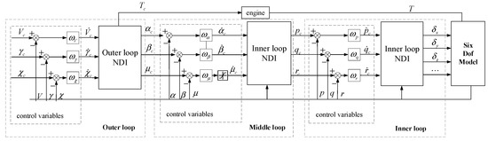
Figure 1.
The structure of the flight control law.
The command of thrust calculated by the flight control law is processed before input into the engine, as shown in Equation (1). Both models of attacker and target are built using the same aerodynamic data and flight control law.
where thr is the actual thrust of the engine, THR is the maximum thrust of the engine.
2.2. Situation Assessment
The coordinate system to evaluate the situation of air combat is shown in Figure 2. VA and VT represent the velocity vectors of the attacker and target, and LOS represents the line of sight from the attacker to the target. The antenna train angle (ATA) represents the deviation angle of the attacker, which is the angle between the velocity vector of the attacker and the line of sight. The aspect angle (AA) represents the deviation angle of the target, which is the angle between the velocity vector of the target and the line of sight. The relationships between the situation parameters are as follows [17]:
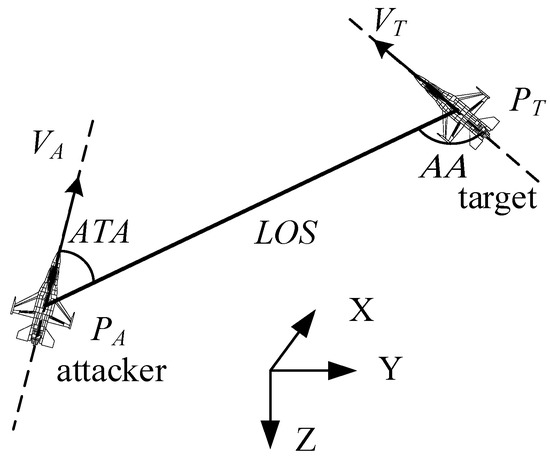
Figure 2.
The coordinate system to evaluate the situation of air combat.
The condition for judging victory in air combat is shown in Equation (6) [2,5,14]. When one party satisfies this condition, it is considered that the party wins.
where the first condition is the constraint on the distance between two aircrafts. When the distance between two aircrafts is greater than the effective range of the missile, the hit rate of the missile is low. However, when the distance between two aircrafts is too small, the missile cannot be launched. In this paper, the effective range of the missile is set to 1000 m, and the minimum launching distance is set to 10 m. The second condition is the constraint of AA; a smaller absolute value of AA indicates that the attacker is at the end of the target, and the attacker is in the advantage. The first two conditions correspond to the no-escape zone of the missile. When the first two conditions are met, no matter how the target maneuvers, it cannot remove the missile launched by the attacker. The third condition is the constraint on ATA; only when ATA is less than the off-axis launch angle of the missile can the missile be launched. In this paper, the maximum angle of the non-escape zone is defined as 60 °, and the maximum off-axis launch angle of the missile is defined as 30°.
2.3. Decision-Making Strategy
The concept of VPPs was first proposed by You et al. [19], and has been widely discussed and studied [20]. The virtual pursuit points include the virtual lag pursuit point, the virtual pure pursuit point, and the virtual lead pursuit point, which correspond to the lag pursuit, the pure pursuit, and the lead pursuit, respectively. By analyzing the turning characteristics, weapon performance, and basic maneuvering principle, the points are generated and transformed into the commands of acceleration using the velocity pursuit guidance law (VPG), and then the commands of overload and rolling angle are obtained based on the aircraft motion equation. The traditional method to obtain the virtual pursuit point is to analyze the flight situation of two aircrafts and the overload of the attacker without considering the long-term benefits; this strategy is usually not optimal. This strategy needs to predict the future position of the target; polynomial fitting was used to predict the positions of the target, but the precision of this method is not enough. The results of air combat are often poor.
When the conventional reinforcement learning method is applied for decision-making in close-range air combat, the commands are generally the aircraft states, such as [V, γ, χ] [17] and [nx, nz, φ] [16], which can be directly connected with the aircraft motion model. Discrete instructions are often used to improve the efficiency of convergence. The amplitude of action is usually fixed, and the number of actions is limited. The effect of the strategy is constrained by the actions, and the maneuverability of the aircraft may not be fully utilized. The results of air combat are often poor.
In the strategy introduced by this paper, the commands are the speed and virtual pursuit points obtained by the reinforcement learning method, and then the virtual pursuit points are converted into the virtual pursuit angles as track angle commands based on the angle guidance law. The efficiency of convergence is good, and the trajectory prediction method combined with BP and LSTM has high accuracy. The track angle commands are continuous, and the amplitudes of them are not fixed, which gives full play to the maneuverability of the aircraft. The results of air combat are often better.
In the air combat strategy based on traditional virtual pursuit points, there is no need for network training as the calculation is simple and the burden of the flight system is low. When the reinforcement learning method is applied, the pre-designed strategy library needs to be loaded, which increases the amount of calculation and puts forward higher requirements for the flight system. The comparisons of the three methods are shown in Figure 3.
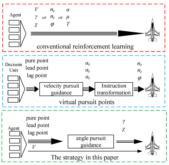
Figure 3.
The comparisons of the three methods.
3. Virtual Lag Points Based on Trajectory Prediction
The pure pursuit, lag pursuit, and lead pursuit correspond to the velocity vector directions of the attacker directly aiming at the target aircraft, the rear, and the front of the target. The lag pursuit point and pure pursuit point can be directly designed based on the current and past positions of the target. The establishment of the lead pursuit point is based on the trajectory prediction of the target. In Ref. [19], polynomial fitting was used to predict the positions of the target, but the precision of this method is not enough, and the choice of the fitting points directly affects the prediction results. In this paper, a trajectory prediction method combining the BP neural network with the LSTM network that considers error prediction, correction, and judgment is proposed, which can greatly improve the prediction accuracy and has high robustness.
3.1. Trajectory Prediction Method
3.1.1. Method and Structure
The structure of the trajectory prediction method considering error prediction, correction, and judgment is shown in Figure 4, including conventional neural network prediction, error prediction, correction, and judgment.
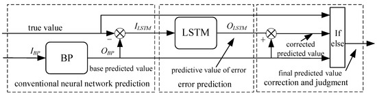
Figure 4.
The structure of the trajectory prediction method.
3.1.2. Conventional Neural Network Prediction
The BP network is a commonly used network with a simple structure and strong robustness that is applied in the conventional prediction module. Unlike traditional trajectory prediction, trajectory prediction in air combat has the characteristics of continuity, mobility, and interactivity. Therefore, the position, track angle, and velocity of the two aircrafts are applied as the input parameters of the neural network, and the output parameters are the position of the target at a certain time in the future. The input and output parameters are normalized to improve accuracy in training, as shown in Equation (7). The structure of the BP neural network is shown in Figure 5.
where V represents the speed of aircraft, γ and χ represent the flight path angle of aircraft, x, y, and z represent the true position on each axis of aircraft, , , and represent the predicted position on each axis of aircraft, and the subscripts b and r represent the blue aircraft and red aircraft.
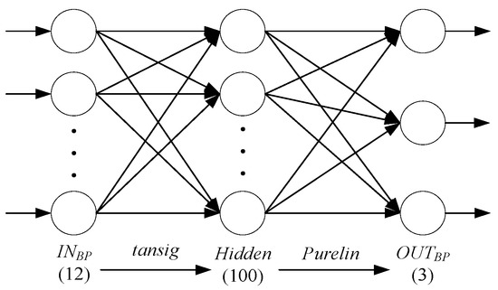
Figure 5.
The structure of the BP neural network.
3.1.3. Error Prediction
The input of the error prediction module is the prediction error of the current and past time, and the output is the error prediction of the next time, as shown in Equation (8), which is time-series data. The LSTM network is a special recurrent neural network that can memorize long-term information and solve long-term dependence problems [21]. Therefore, the LSTM network is applied in the error prediction module, and the structure of the network is shown in Figure 6.
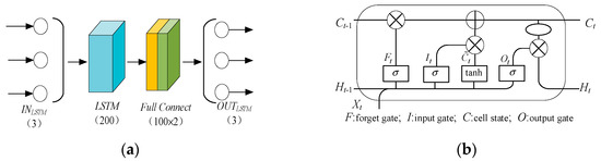
Figure 6.
The structure of the LSTM network. (a) Predicting network. (b) The neural unit of LSTM.
3.1.4. Correction and Judgment
The corrected prediction value is the superposition of the output of the basic prediction module and the output of the error prediction module. However, to ensure the accuracy of the prediction results and improve the robustness, the basic prediction value and the corrected prediction value are judged before the output results, and the logic of the module is shown in Equation (9). If the error of the basic prediction value is less than that of the corrected prediction value, the basic prediction effect in the past temp is better than the corrected result, the basic prediction value is the output, otherwise the corrected prediction value is the output.
where cpv represents the corrected prediction value; bpv represents the basic prediction value; fpv represents the final prediction value; and tv represents the true value.
3.2. Prediction Results
A total of 5000 sets of air combat data are obtained by mathematical simulation; 70% of the data are used as the training set, and the remaining 30% are used as the test set.
By changing the parameters of the non-linear dynamic inverse flight control law, the motion characteristics and agility of the aircraft can be changed. Before each air combat simulation, the flight control law parameters of two aircrafts are randomly given, as shown in Equation (10), so as to simulate the aircraft of agility with different motion characteristics in air combat [17]. Other parameters of the flight control law remain unchanged with the recommended values in Section 2.1.
Before each air combat simulation, the initial speed, heading, and position of two aircrafts are randomly given, as shown in Equation (11), so as to simulate an aircraft with different states in air combat.
According to the existing research results [17,19], the air combat strategy library has been established, including the ADP strategy and the guidance law using virtual pursuit points. Before each air combat simulation, the air combat strategies of two aircrafts are randomly selected. The initial speed, heading, position, motion characteristics, and air combat strategy of two aircrafts are all given randomly, so as to approximate the actual air combat situation as much as possible and improve the relevance of the data set.
The predicted values are the positions of the target after 1 s, 2 s, and 3 s in the future; the changes in the evaluation parameters during training are shown in Figure 7.
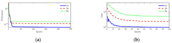
Figure 7.
The changes in evaluation parameters during training (a) BP (learning rate = 0.005); (b) LSTM (learning rate = 0.005).
The air combat data of the test set are selected and predicted using the conventional BP network, the polynomial fitting, and the BP-LSTM network with an error prediction, correction, and judgment function proposed in this paper; the predicted values are the position of the target after 1 s in the future. The results of the three methods are compared, as shown in Figure 8.
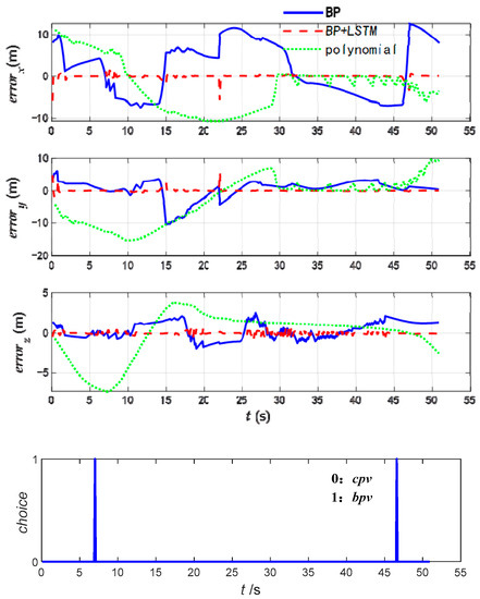
Figure 8.
The results of the three methods.
When the conventional BP neural network is applied, the maximum errors of the x, y, and z axis are 12.69 m, 10.57 m, and 2.59 m, and the average errors are 5.92 m, 2.21 m, and 0.94 m. When the conventional polynomial fitting is applied, the maximum errors of the x, y, and z axis are 11.34 m, 21.07 m, and 14.32 m, and the average errors are 4.79 m, 5.03 m, and 4.81 m. However, the maximum errors of the x, y, and z axis are 5.82 m, 5.80 m, and 0.80 m when the BP-LSTM neural network is applied, and the average errors are 0.22 m, 0.15, and 0.15 m. In the process of prediction, only two outputs are the basic prediction values, and the other outputs are the corrected prediction values.
The indexes of the mean absolute error (MAE) and root mean square error (RMSE) are applied to evaluate the prediction results of all the test sets. The definition of indexes is shown in Equation (12). The prediction results of the evaluation are shown in Figure 9.
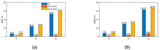
Figure 9.
The MAE and RMSE of the prediction results. (a) MAE; (b) RMSE.
When the BP-LSTM neural network is applied, compared with the conventional polynomial fitting, the MAE of the trajectory prediction results after 1 s, 2 s, and 3 s in the future decreased, respectively, by 94.4%, 96.1%, and 96.2%; the RMSE of the trajectory prediction results after 1 s, 2 s, and 3 s in the future decreased, respectively, by 81.4%,89.4%, and 89.6%. Compared to the conventional BP neural network, the MAE of the prediction results decreased, respectively, by 93.3%, 95.8%, and 95.8%; the RMSE of the prediction results decreased, respectively, by 79.9%, 88.6%, and 89.1%.
Therefore, the trajectory prediction method combining the BP neural network with the LSTM network that considers error prediction, correction, and judgment can significantly improve the accuracy of the prediction accuracy. The positions of the target predicted by this method can be used as the virtual lead points. It is worth noting that this method is generally applicable to the trajectory prediction, and the network structure chosen for the conventional prediction module and the error prediction module can be changed according to the needs of the study.
4. Strategy Training
The traditional method used to obtain the virtual pursuit point analyzes the flight situation of two aircrafts and the overload of the attacker without considering the long-term benefits; this strategy is usually not optimal. In this paper, a strategy that chooses the virtual pursuit points and speed by reinforcement learning method is proposed, and the virtual pursuit points are converted into the virtual pursuit angles as the commands of track angles using the angle guidance law. The selection of commands is linked to current and future rewards and the long-term benefits are considered.
4.1. Markov Decision Model
The Markov decision model is the basis of the decision-making strategy that uses the reinforcement learning method. It is necessary to determine the state, action, state transition function, and reward function of the Markov decision model in close-range air combat.
4.1.1. States
In the process of close-range air combat, a certain state of the Markov decision model includes the flight status and the relative situation of the two aircrafts. The states (s) of air combat used in this paper are shown in Equation (13) and have been normalized to improve the convergence efficiency of the strategy.
4.1.2. Actions and State Transition Functions
The actions of the strategy designed in this paper are virtual pursuit angles and speeds. The virtual pursuit angles are converted by virtual pursuit points using the angle guidance law. The virtual pursuit points include a pure pursuit point, two lag pursuit points, and three lead points, which are the current position of the aircraft, the position before 1 s and 2 s, and the predicted position after 1 s, 2 s, and 3 s, respectively. The command of speed is expressed by the rate of change, and the specific value is shown in Equation (14).
The virtual pursuit points cannot be directly applied to aircraft models in close-range air combat, so they are converted into the virtual pursuit angles as the command of track angles using the angle guidance law. The actions and state transition functions as shown in Equation (15) are as follows:
where the superscript t represents the current time and is the decision step.
4.1.3. Reward
The design of the reward function directly affects the training effect of the strategy. The reward in the process of close-range air combat includes an immediate reward and a situational reward.
The function of the immediate reward value can be expressed as follows [5]:
The function of the situational reward can be expressed as follows [17]:
In the process of air combat, our aircraft (blue aircraft) needs to quickly seize the advantage position while avoiding being in a disadvantageous position. Therefore, the reward function of close air combat can be expressed as follows:
In the function, d is the optimal launching distance of the close-range missile, k is the weight used to adjust the importance of the distance advantage and the angle advantage, and q is the weight used to adjust the importance of the immediate reward and the situational reward. In this paper, d = 500 m, k = 10 m, and q = 0.5.
4.2. Training Algorithm
The mainstream algorithms in reinforcement learning, such as DDPG, TD3, PPO, and so on, have been widely applied in air combat. The PPO is a random strategy algorithm with strong robustness, which is excellent in terms of sampling efficiency and algorithm performance. It is the preferred algorithm of open AL. Therefore, the PPO is applied to train the decision-making strategy for close-range air combat, and the actions are virtual pursuit points and velocity. The process of PPO is shown in Algorithm 1 [22].
| Algorithm 1: PPO. |
| for iteration = 1.2… do |
| for actor = 1, 2, …, N do |
| Run policy πθold in the environment for T timesteps |
| Compute advantage estimate . ⋯; |
| end for |
| Optimize surrogate L wrt θ, with K epochs and minibatch size M < NT |
| θold ← θ |
| end for |
Here, N is the number of parallel actors, t is the timestep, K is the epoch number, M is the minibatch size, πθ is the stochastic policy, is the estimation of the advantage function at timestep t, L is the surrogate objective, and θ is the vector of the policy parameters.
The structure of the network in the PPO algorithm is shown in Figure 10. The training results are shown in Figure 11. The learn rate for actor is 0.0001, the learn rate for critic is 0.001, and the window length for averaging is 600.
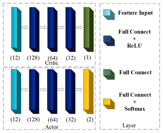
Figure 10.
Structure of network in the PPO algorithm.
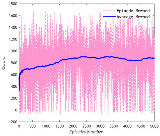
Figure 11.
The training results.
5. Simulation and Analysis
Mathematical simulations are carried out based on the close-range air combat model established above, and the superiority and effectiveness of the strategy with virtual pursuit angles and speed as variable-scale actions are verified by comparing the air combat results. The body model and flight control laws of two aircrafts are the same, as described in Section 2.1. In the mathematical simulation, Runge–Kutta (P-K) of order four methods was applied to solve the differential equations. The fixed simulation step is 0.02 s, the maximum time of the simulation is 120 s, so if one aircraft wins in the specified time, the simulation is over, and the decision step is 0.02 s, which is compatible with the time step used for the mathematical simulation.
5.1. Typical Scenes
The typical initial scenes of air combat can be divided into four categories: blue in advantages, blue in disadvantages, two aircrafts in parallel flight, and two aircrafts in opposite flight, as shown in Figure 12. The strategy of close-range air combat established in this paper is applied by blue aircraft and the strategy with a fixed amplitude of the actions obtained by conventional reinforcement learning is applied by red aircraft. The algorithm applied by the red aircraft is also PPO, and the actions are the change rate of velocity and track angle commands, as shown in Equation (19):
where ΔVc [−10 m/s, 0, 10 m/s], Δγc [−5°, 0, 5°], and Δχc [−20°, 0, 20°].
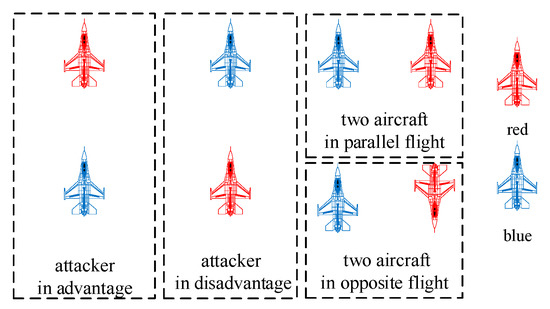
Figure 12.
Initial scenes.
The initial state of the two aircrafts in four simulation scenarios is shown in Table 1.

Table 1.
The initial state of the two aircrafts in four scenarios.
5.1.1. Blue Aircraft in Advantage
At the beginning of the combat, the red aircraft turned and climbed. The blue aircraft followed the red aircraft and won at 38.6 s. The trajectories of the two aircrafts during air combat are shown in Figure 13.
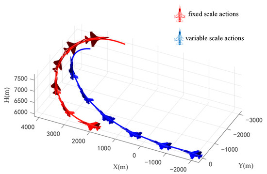
Figure 13.
Trajectories of two aircrafts when blue aircraft in advantage.
The commands and responses of the track angles of the two aircrafts during the combat are shown in Figure 14, the change rate of track angle commands are shown in Figure 15, and the comparisons of typical flight parameters are shown in Figure 16.
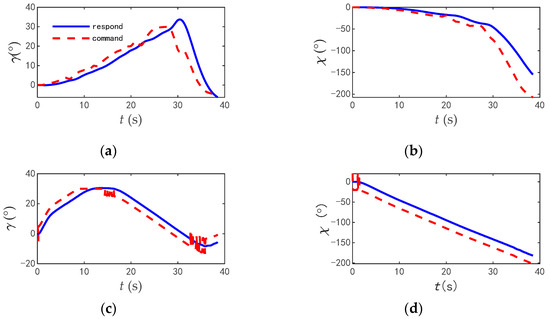
Figure 14.
The commands and responses of the track angle when blue aircraft in advantage. (a) Track inclination angle of blue aircraft. (b) Track deflection angle of blue aircraft. (c) Track inclination angle of red aircraft. (d) Track deflection angle of red aircraft.
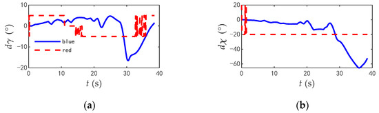
Figure 15.
The change rate of track angle commands when blue aircraft in advantage. (a) Track inclination angle of two aircrafts. (b) Track deflection angle of two aircrafts.
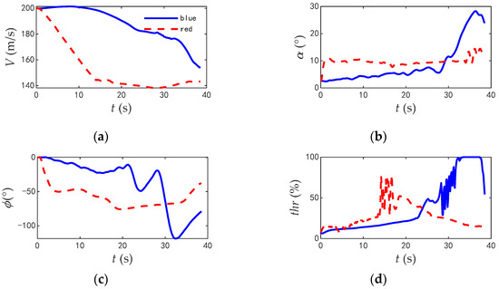
Figure 16.
The comparison of typical flight parameters when blue aircraft in advantage. (a) Velocity. (b) Angle of attack. (c) Roll angle. (d) Thrust.
According to the flight parameters of the two aircrafts, the red aircraft was at a disadvantage at the initial time, attempting to obtain an angle advantage by turning to the tail of the blue aircraft and a height advantage by improving its height. During the turning process, the velocity of the red aircraft rapidly reduced and the roll angle of the red aircraft increased to reduce the turning radius. However, due to the amplitude of the command variable being fixed, the red aircraft could not give full play to its maneuverability. The maximum roll angle was 77.2°, and the angle of attack was always less than 15°. The engine thrust never reached its extreme value, and the average utilization rate of thrust was 27.2%. In contrast, the blue aircraft accelerated at the beginning of the combat to shorten the distance between the two aircrafts, and tightly bit the tail of the red aircraft. At 28.3 s, the blue aircraft quickly climbed and rolled to change course. The maximum roll angle was 118.6°, and the maximum angle of attack was 28.2°. The time for the engine to reach full thrust was 4.1 s, and the average utilization rate of thrust was 37.9%. The blue aircraft gave full play to the maneuverability of the aircraft.
5.1.2. Blue Aircraft in Disadvantage
At the beginning of the combat, the blue aircraft quickly turned and inserted into the inside of the red aircraft and won at 73.7 s. The trajectories of the two aircrafts during air combat are shown in Figure 17.
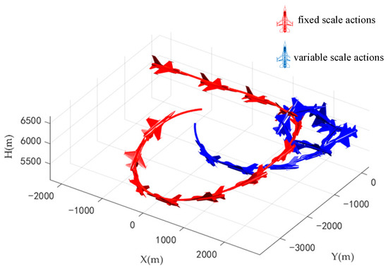
Figure 17.
Trajectories of two aircrafts when blue aircraft in disadvantage.
The commands and responses of the track angles of the two aircrafts during the combat are shown in Figure 18; the change rate of track angle commands are shown in Figure 19; and the comparisons of typical flight parameters are shown in Figure 20.
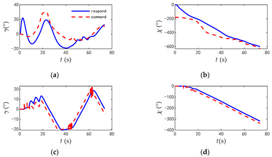
Figure 18.
The commands and responses of the track angle when blue aircraft in disadvantage. (a) Track inclination angle of blue aircraft. (b) Track deflection angle of blue aircraft of blue aircraft. (c) Track inclination angle of red aircraft. (d) Track deflection angle of blue aircraft of red aircraft.
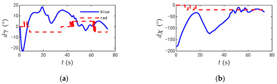
Figure 19.
The change rate of track angle commands when blue aircraft in disadvantage. (a) Track inclination angle of two aircrafts. (b) Track deflection angle of blue aircraft of two aircrafts.
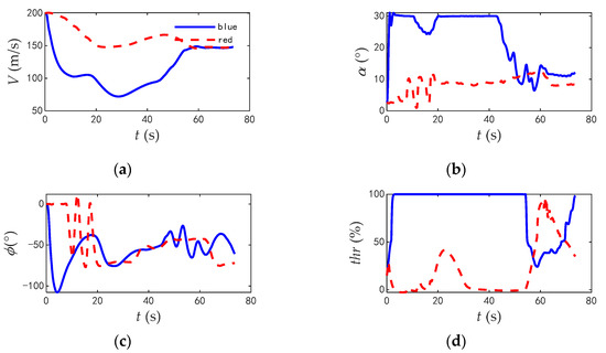
Figure 20.
The comparison of typical flight parameters when blue aircraft in disadvantage. (a) Velocity. (b) Angle of attack. (c) Roll angle. (d) Thrust.
According to the flight parameters of the two aircrafts, the red aircraft was at an advantage at the initial time and kept flying flat at the beginning to shorten the distance. In contrast, the blue aircraft rapidly reduced its velocity and rolled quickly, intending to reduce the danger by turning with the minimum radius. The maximum roll angle was 107.7°, and the maximum angle of attack reached 30° (the limit value of flight control system). The time taken to change the track deflection angle from 0° to 180° was 15.6 s, and the time taken to change the track deflection angle from 0° to 360° was 36.7 s. The average utilization rate of thrust during combat was 84.7%. The blue aircraft gave full play to the maneuverability of the aircraft. However, the attack angle of the red aircraft was always lower than 15°, and the average utilization rate of thrust was only 20.43%, which does not give full play to the maneuverability of the aircraft.
5.1.3. Two Aircrafts in Parallel Flight
At the beginning of the combat, the same maneuver was used by the two aircrafts, but the blue aircraft quickly turned to the inside of the red aircraft and won at 29.5 s. The trajectories of the two aircrafts during air combat are shown in Figure 21.
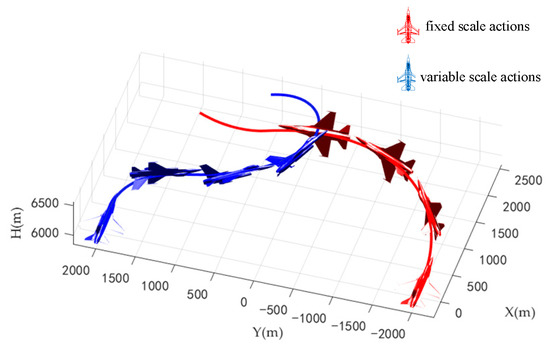
Figure 21.
Trajectories of two aircrafts when two aircrafts in parallel flight.
The commands and responses of the track angles of the two aircrafts during the combat are shown in Figure 22; the change rate of track angle commands are shown in Figure 23; and the comparisons of typical flight parameters are shown in Figure 24.
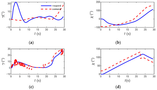
Figure 22.
The commands and responses of the track angle when two aircrafts in parallel flight. (a) Track inclination angle of blue aircraft. (b) Track deflection angle of blue aircraft of blue aircraft. (c) Track inclination angle of red aircraft. (d) Track deflection angle of blue aircraft of red aircraft.

Figure 23.
The change rate of track angle commands when two aircrafts in parallel flight. (a) Track inclination angle of two aircrafts. (b) Track deflection angle of blue aircraft of two aircrafts.
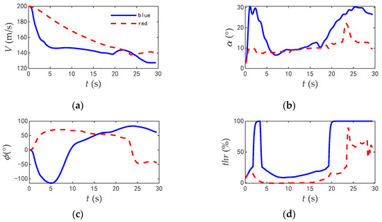
Figure 24.
The comparison of typical flight parameters when two aircrafts in parallel flight. (a) Velocity; (b) Angle of attack. (c) Roll angle; (d) Thrust.
According to the flight parameters of the two aircrafts, both two aircrafts chose to reduce the velocity and turned at the beginning of the combat. However, limited by the fixed amplitude of the actions, the track deflection angle command at the initial time of the red aircraft is 20°, while that of the blue aircraft is −90°. More of the blue aircraft’s energy is used for turning. During the turning process, the maximum roll angle of the blue aircraft was 114.6°, the maximum angle of attack was 31.1°, the time for the engine to reach full thrust was 14.8 s, and the average utilization rate of thrust is 76.2%. The blue aircraft gave full play to the maneuverability of the aircraft. The red aircraft turned slowly, and the maximum roll angle was only 73.5°, and the maximum angle of attack was 21.8°. The time of the engine to reach full thrust was 7.2 s, and the average utilization rate of thrust is 36.3%. Therefore, the blue aircraft first turned to the tail of the red aircraft and won.
5.1.4. Two Aircrafts in Opposite Flight
At the beginning of the combat, the two aircrafts were flying flat to shorten the distance, and then the red aircraft climbed. The blue aircraft turned quickly and always followed the red aircraft to win at 63.2 s. The trajectories of two aircrafts during air combat are shown in Figure 25.
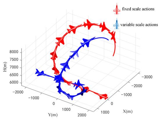
Figure 25.
Trajectories of two aircrafts when two aircrafts in opposite flight.
The commands and responses of the track angles of the two aircrafts during the combat are shown in Figure 26, the change rate of track angle commands are shown in Figure 27, and the comparisons of typical flight parameters are shown in Figure 28.
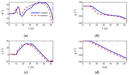
Figure 26.
The commands and responses of the track angle when two aircrafts in opposite flight. (a) Track inclination angle of blue aircraft; (b) Track deflection angle of blue aircraft of blue aircraft. (c) Track inclination angle of red aircraft; (d) Track deflection angle of blue aircraft of red aircraft.
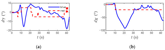
Figure 27.
The change rate of track angle commands when two aircrafts in opposite flight. (a) Track inclination angle of two aircrafts. (b) Track deflection angle of blue aircraft of two aircrafts.
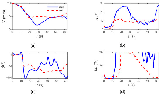
Figure 28.
The comparison of typical flight parameters when two aircrafts in opposite flight. (a) Velocity. (b) Angle of attack. (c) Roll angle. (d) Thrust.
According to the flight parameters of the two aircrafts, in the early stages of combat, the two aircrafts chose to fly straight to shorten the distance, and then they climbed up to increase the height and turned to obtain the angle advantage. However, the initial roll angle of the red aircraft was only 48.9°, the maximum roll angle was only 77.7°, and the maximum angle of attack was 12.1°. The time taken for the engine to reach full thrust was 6.5 s, and the average utilization rate of thrust was 40.5%. While the initial roll angle of the blue aircraft was 103.6°, the maximum angle of attack was 27.6°, the time for the engine to reach full thrust was 33.7 s, and the average utilization rate of thrust was 74.7%.
Therefore, the decision-making strategy for close-range air combat based on reinforcement learning with variable-scale actions can give full play to the maneuverability and agility of the aircraft and gain advantages as quickly as possible in the process of combat.
5.2. Monte Carlo Mathematical Simulation
To further evaluate the effectiveness and excellence of the strategy proposed in this paper, the strategy with virtual pursuit angles and speed as actions and the strategy with fixed amplitude of actions were, respectively, applied by the blue aircraft, and the strategy of ADP was applied by the red aircraft. The data of 1000 air combats were obtained based on the Monte Carlo mathematical simulation, and the initial states of the two aircrafts were randomly generated according to Equation (11) in Section 3.2. The maximum time of each simulation is still 120 s, so if one aircraft wins in the specified time, the simulation is over; otherwise, the two aircrafts will be considered tied.
The results of air combat under different strategies are shown in Figure 29 and Figure 30. In 1000 air combat games, when the conventional strategy is applied by the blue aircraft, the percentage of wins for the blue aircraft is 39.8%, the percentage for the red aircraft is 23.5%, and the percentage for both sides drawing is 37.2%. The median time taken for the blue aircraft to capture the red aircraft is 67.1 s, and the median time taken for the red aircraft to capture the blue aircraft is 42.3 s. When the strategy with virtual pursuit angles and speed as actions is applied by the blue aircraft, the percentage of wins for the blue aircraft is 54.1%, the percentage for the red aircraft is 2.8%, and the percentage for both sides drawing is 42.9%. The median time taken for the blue aircraft to capture the red aircraft is 38.6 s, and the median time taken for the red aircraft to capture the blue aircraft is 47.0 s. Compared with the conventional strategy, the success rate of attack increased by 14.5%; the success rate of defense increased by 21.7%. The median time taken for the blue aircraft to capture the red aircraft was reduced by 38.3 s, and the median time for the red aircraft to capture the blue aircraft increased by 4.7 s. Therefore, the effectiveness and excellence of the strategy with virtual pursuit angles and speed as actions can be observed.

Figure 29.
The winning rate under different strategies.
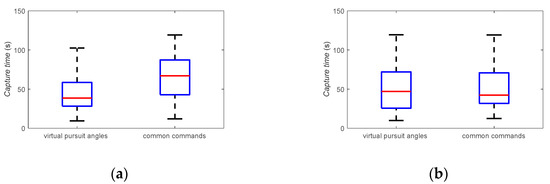
Figure 30.
The median time under different strategies. (a) Blue win. (b) Blue lose.
6. Conclusions
This paper designs a decision-making strategy for close-range air combat based on reinforcement learning with variable-scale actions. The actions are not the common fixed-amplitude commands but the variable-scale virtual pursuit angles and speeds. Predicting target aircraft coordinates is the premise of calculating virtual pursuit angles. The trajectory prediction method, combining the BP neural network with the LSTM network that considers error prediction, correction, and judgment, is applied to predict the coordinates of the target aircraft to achieve higher accuracy. When the BP-LSTM neural network is applied, compared to the conventional polynomial fitting, the MAE of the trajectory prediction results after 1 s, 2 s, and 3 s in the future decreased, respectively, by 94.4%, 96.1%, and 96.2%; the RMSE of the trajectory prediction results after 1 s, 2 s, and 3 s in the future decreased, respectively, by 81.4%, 89.4%, and 89.6%. Compared to the conventional BP neural network, the MAE of the trajectory prediction results decreased, respectively, by 93.3%, 95.8%, and 95.8%; the RMSE of the trajectory prediction results decreased, respectively, by 79.9%, 88.6%, and 89.1%.
The simulation results of 1000 air combats show that the strategy with virtual pursuit angles and speed can give full play to the maneuverability and agility of the aircraft in the process of engagement. Compared with the conventional strategy of actions with a fixed amplitude, when the strategy with virtual pursuit angles and speed as the action is applied in air combat, the angle of attack, roll angle, and thrust utilization rate of an aircraft are all high. The success rate of attack increases by about 15 percentage points, the success rate of defense increases by about 22 percentage points, and the time spent capturing the enemy aircraft decreases by about 50%.
Author Contributions
Conceptualization, L.W. and J.W.; methodology, J.W.; software, J.W.; validation, L.W., J.W. and H.L.; formal analysis, T.Y.; investigation, T.Y.; resources, H.L.; data curation, J.W.; Writing—original draft preparation, L.W., J.W., H.L. and T.Y.; Writing—review and editing, L.W., J.W., H.L. and T.Y.; visualization, J.W.; supervision, L.W.; project administration, L.W.; funding acquisition, L.W. All authors have read and agreed to the published version of the manuscript.
Funding
This research received no external funding.
Data Availability Statement
No new data were created or analyzed in this study. Data sharing is not applicable to this article.
Conflicts of Interest
The authors declare no conflict of interest.
References
- Pan, Q.; Zhou, D.Y.; Huang, J.C.; Lv, X.F.; Yang, Z.; Zhang, K.; Li, X.Y. Maneuver Decision for Cooperative Close-Range Air Combat Based on State Predicted Influence Diagram. In Proceedings of the IEEE International Conference on Information and Automation (ICIA), Macau, China, 18–20 July 2017; pp. 726–731. [Google Scholar]
- Jiandong, Z.; Qiming, Y.; Guoqing, S.; Yi, L.; Yong, W. UAV cooperative air combat maneuver decision based on multi-agent reinforcement learning. J. Syst. Eng. Electron. 2021, 32, 1421–1438. [Google Scholar] [CrossRef]
- Park, H.; Lee, B.Y.; Tahk, M.J.; Yoo, D.W. Differential Game Based Air Combat Maneuver Generation Using Scoring Function Matrix. Int. J. Aeronaut. Space Sci. 2016, 17, 204–213. [Google Scholar] [CrossRef]
- Sun, Y.-Q.; Zhou, X.-C.; Meng, S.; Fan, H.-D. Research on Maneuvering Decision for Multi-fighter Cooperative Air Combat. In Proceedings of the 2009 International Conference on Intelligent Human-Machine Systems and Cybernetics, Hangzhou, China, 26–27 August 2009; pp. 197–200. [Google Scholar] [CrossRef]
- McGrew, J.S.; How, J.P.; Williams, B.; Roy, N. Air-Combat Strategy Using Approximate Dynamic Programming. J. Guid. Control Dyn. 2010, 33, 1641–1654. [Google Scholar] [CrossRef]
- Li, N.; Yi, W.Q.; Gong, G.H. Multi-aircraft Cooperative Target Allocation in BVR Air Combat Using Cultural-Genetic Algorithm. In Proceedings of the Asia Simulation Conference/International Conference on System Simulation and Scientific Computing (AsiaSim and ICSC 2012), Springer-Verlag Berlin, Shanghai, China, 27–30 October 2012; pp. 414–422. [Google Scholar]
- Duan, H.; Pei, L.; Yu, Y. A Predator-prey Particle Swarm Optimization Approach to Multiple UCAV Air Combat Modeled by Dynamic Game Theory. IEEE/CAA J. Autom. Sin. 2015, 2, 11–18. [Google Scholar] [CrossRef]
- Huang, C.; Dong, K.; Huang, H.; Tang, S. Autonomous air combat maneuver decision using Bayesian inference and moving horizon optimization. J. Syst. Eng. Electron. 2018, 29, 86–97. [Google Scholar] [CrossRef]
- Burgin, G.H.; Fogel, L.J. Air-to-Air Combat Tactics Synthesis and Analysis Program Based on An Adaptive Maneuvering Logic, NASA. J. Cybern. 1972, 2, 60–68. [Google Scholar] [CrossRef]
- He, X.; Zu, W.; Chang, H.; Zhang, J.; Gao, Y. Autonomous Maneuvering Decision Research of UAV Based on Experience Knowledge Representation. In Proceedings of the 28th Chinese Control and Decision Conference, Yinchuan, China, 28–30 May 2016; pp. 161–166. [Google Scholar]
- Hu, D.; Yang, R.; Zuo, J.; Zhang, Z.; Wu, J.; Wang, Y. Application of Deep Reinforcement Learning in Maneuver Planning of Beyond-Visual-Range Air Combat. IEEE Access 2021, 9, 32282–32297. [Google Scholar] [CrossRef]
- You, S.X.; Diao, M.; Gao, L.P.; Zhang, F.L.; Wang, H. Target tracking strategy using deep deterministic policy gradient. Appl. Soft Comput. 2020, 95, 13. [Google Scholar] [CrossRef]
- Qiu, X.; Yao, Z.; Tan, F.; Zhu, Z.; Lu, J.-G. One-to-one Air-combat Maneuver Strategy Based on Improved TD3 Algorithm. In Proceedings of the 2020 Chinese Automation Congress (CAC), Shanghai, China, 6–8 November 2020; pp. 5719–5725. [Google Scholar] [CrossRef]
- Kong, W.R.; Zhou, D.Y.; Zhang, K.; Yang, Z. Air combat autonomous maneuver decision for one-on-one within visual range engagement base on robust multi-agent reinforcement learning. In Proceedings of the 16th IEEE International Conference on Control and Automation (ICCA)Electr Network, Singapore, 9–11 October 2020; pp. 506–512. [Google Scholar]
- Sun, Z.X.; Piao, H.Y.; Yang, Z.; Zhao, Y.Y.; Zhan, G.; Zhou, D.Y.; Meng, G.L.; Chen, H.C.; Chen, X.; Qu, B.H.; et al. Multi-agent hierarchical policy gradient for Air Combat Tactics emergence via self-play. Eng. Appl. Artif. Intell. 2021, 98, 14. [Google Scholar] [CrossRef]
- Austin, F.; Carbone, G.; Falco, M.; Hinz, H.; Lewis, M. Automated maneuvering decisions for air-to-air combat. In Proceedings of the Guidance, Navigation and Control Conference, Monterey, CA, USA, 17–19 August 1987. [Google Scholar] [CrossRef]
- Wang, M.; Wang, L.; Yue, T.; Liu, H. Influence of unmanned combat aerial vehicle agility on short-range aerial combat effectiveness. Aerosp. Sci. Technol. 2020, 96, 105534. [Google Scholar] [CrossRef]
- Sonneveldt, L. Nonlinear F-16 Model Description; Delft University of Technology: Delft, The Netherlands, 2006. [Google Scholar]
- You, D.-I.; Shim, D.H. Design of an aerial combat guidance law using virtual pursuit point concept. Proc. Inst. Mech. Eng. Part G J. Aerosp. Eng. 2014, 229, 792–813. [Google Scholar] [CrossRef]
- Shin, H.; Lee, J.; Kim, H.; Shim, D.H. An autonomous aerial combat framework for two-on-two engagements based on basic fighter maneuvers. Aerosp. Sci. Technol. 2018, 72, 305–315. [Google Scholar] [CrossRef]
- Yu, Y.; Si, X.S.; Hu, C.H.; Zhang, J.X. A Review of Recurrent Neural Networks: LSTM Cells and Network Architectures. Neural Comput. 2019, 31, 1235–1270. [Google Scholar] [CrossRef] [PubMed]
- Wang, Z.; Li, H.; Wu, Z.; Wu, H. A pretrained proximal policy optimization algorithm with reward shaping for aircraft guidance to a moving destination in three-dimensional continuous space. Int. J. Adv. Robot. Syst. 2021, 18, 1–13. [Google Scholar] [CrossRef]
Disclaimer/Publisher’s Note: The statements, opinions and data contained in all publications are solely those of the individual author(s) and contributor(s) and not of MDPI and/or the editor(s). MDPI and/or the editor(s) disclaim responsibility for any injury to people or property resulting from any ideas, methods, instructions or products referred to in the content. |
© 2023 by the authors. Licensee MDPI, Basel, Switzerland. This article is an open access article distributed under the terms and conditions of the Creative Commons Attribution (CC BY) license (https://creativecommons.org/licenses/by/4.0/).