Analytical Redundancy for Variable Cycle Engine Based on Variable-Weights-Biases Neural Network

Abstract

Due to the complex nature of a variable cycle engine (VCE), which has numerous control variables and working modes across a broad flight envelope, coupled with the whole engine’s degradation, the analytical redundancy method based on component-level models may not provide an accurate estimation of the sensors. Variable-weights-biases neural network (VWB Net) is proposed to construct VCE’s analytical redundancy. Unlike conventional networks whose weights and biases are fixed, VWB Net’s variable-weights and variable-biases are functions of input which greatly increase its nonlinear mapping capability by integrating input information. Variable-biases can also be used to eliminate the error between actual sensor output and estimated value quickly at the terminal node. Compared with the BP network and Dense net, VWB Net has fewer parameters, faster calculation speed, and higher accuracy. Digital simulation results of VCE parameter estimation demonstrate that VWB Net’s average relative errors are under 0.27% with calculation and parameter efficiency at least 166 times higher than that of Dense net. Hardware in the loop simulation further verifies VWB Net’s estimation accuracy and real-time calculation.

1. Introduction

Compared with conventional gas turbine engines, VCE has more sophisticated structures and more working modes, operating in a broader flight envelope and power range [1,2]. It is necessary for the engine through the fault-tolerant control (FTC) system to ensure safe and stable operation [3]. Engine sensors can fail under harsh conditions, such as high-temperature and high-pressure environments. Two primary redundancy techniques used by the engine FTC system are hardware redundancy and analytical redundancy [4,5]. Compared with hardware redundancy, analytical redundancy reduces the number of sensors measuring the same physical variable which is of great significance for simplified design and weight reduction of aeroengine [6,7]. The operation of aeroengine produces a significant amount of pollutants [8]. By utilizing analytical redundancy techniques, it is possible to reduce the weight of the engine, thereby achieving the goal of reducing emissions.

Analytical redundancy techniques can be divided into two categories: model-based methods and data-driven methods [9,10,11,12]. The engine component-level model method combined with the Kalman filter [13,14] is the most commonly used model-based method. Given that it is not easy to build an accurate engine dynamic model with performance degradation, the Kalman filter is adopted to improve the adaptation of the engine model [15,16]. Since VCE is a more complicated nonlinear power system across a broader flight envelope and power range, in the absence of accurate component characteristics, the adaptive model based on the component-level model cannot accurately track engine outputs in case more components have degenerated [17].

The data-driven method provides a promising solution for analytical redundancy which can extract the engine features and bridge the relationship between input and output from a large number of experimental data. Shallow learning methods, such as support vector machine (SVM) [18,19,20] and extreme learning machine (ELM) [21,22], have quick calculation speed; however, they cannot extract deep information. Jun Zhou et al. [21] proposed an ELM-based method to provide analytical redundancy for sensor fault diagnostics. In Zhao’s simulation, there are very few input variables, working range, and degradation parameters. Deep learning methods are precisely the product of solving highly nonlinear problems [23,24]. Deep learning methods, such as LSTM [25], Resnet [26], and Google net [27], are widely used to solve regression problems. The layers of these networks range from dozens to hundreds, and the parameters of the Dense net even exceed ten million which result in large storage cost and slow calculation speed [28]. The control parameters of VCE increase by 40% compared with traditional engines [29], so the mapping relationship among variables is more complex. Most data-driven methods based on machine learning algorithms encounter the problem that learning accuracy and calculation speed cannot be satisfied at the same time [30].

In order to solve the problems of low accuracy caused by the simple structure of shallow learning network and the slow speed of online operation caused by the complex topology of a deep learning network, the variable-weights-biases neural network is proposed to construct the analytical redundancy for variable cycle engine. The proposed network’s variable-weights and variable-biases are nonlinear mappings of input variables that can realize complete information fusion from different variables and helps neurons fit out the nonlinear relationship among VCE variables more quickly and accurately. Additionally, variable-biases can be used at the terminal node to quickly remove the discrepancy between the actual sensor output and estimated value. The nonlinear expressive capability of the VWB Net significantly increases while the number of parameters is decreased so the network calculates faster.

The remainder of the paper is organized as follows: Section 2.1 gives the core principle of VWB Net, Section 2.2 introduces the structure of the variable-weights-biases neural network (VWB Net), and Section 2.3 introduces the structure of the variable cycle engine. In Section 3.1 and Section 3.2, the digital simulation experiments are conducted to demonstrate the performance of the VWB Net and VWB Net are compared with BP neural network (BPNN) and Dense net [28]. The experiment situation is accompanied by the whole engine’s degradation across a broad flight envelope. Section 3.3 introduces the framework of the hardware in the loop (HIL) simulation experiment. In Section 3.4, VWB Net’s estimation accuracy and real-time performance are verified in the HIL simulation experiment. Section 4 presents a summary of the results and conclusions.

2. Method

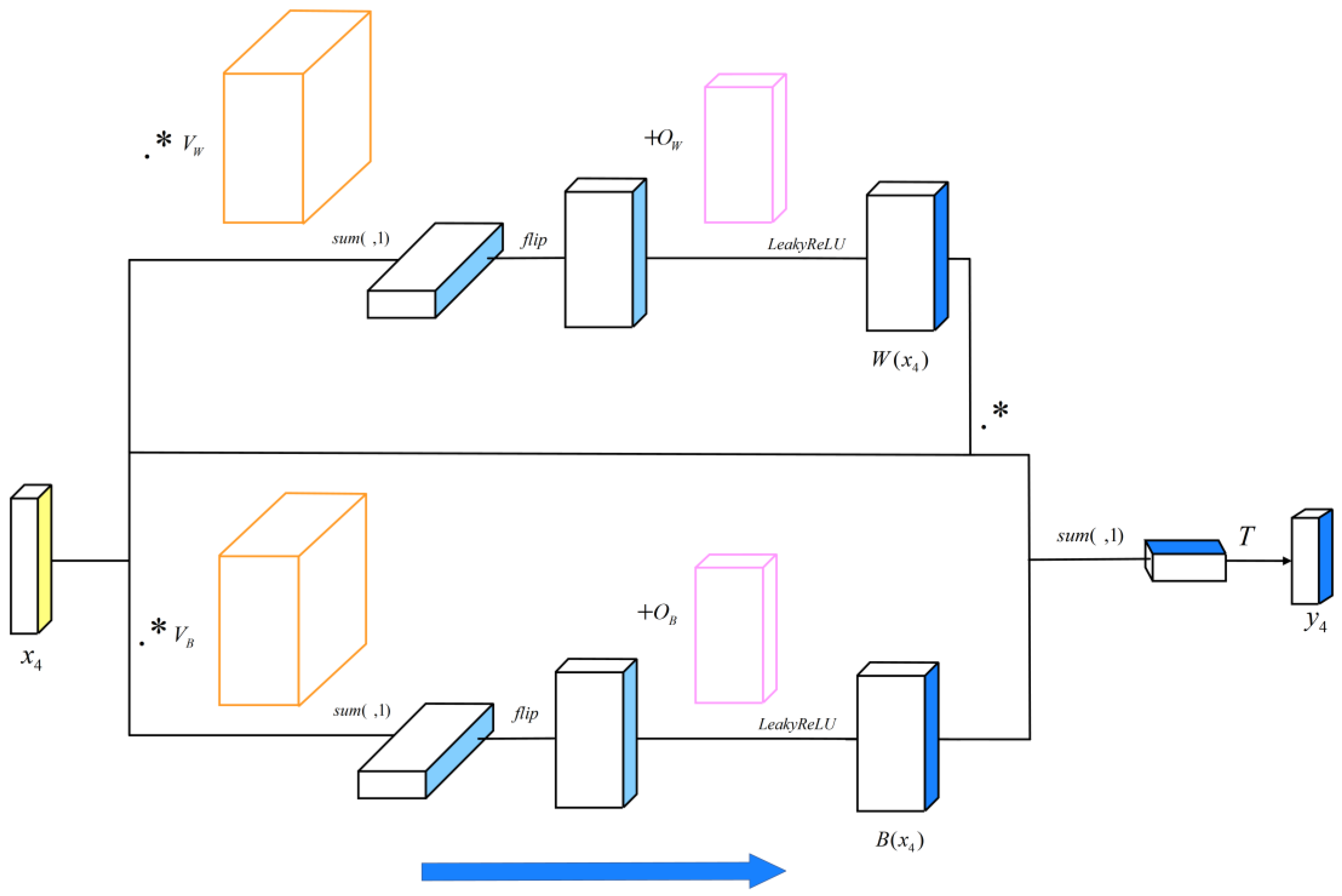
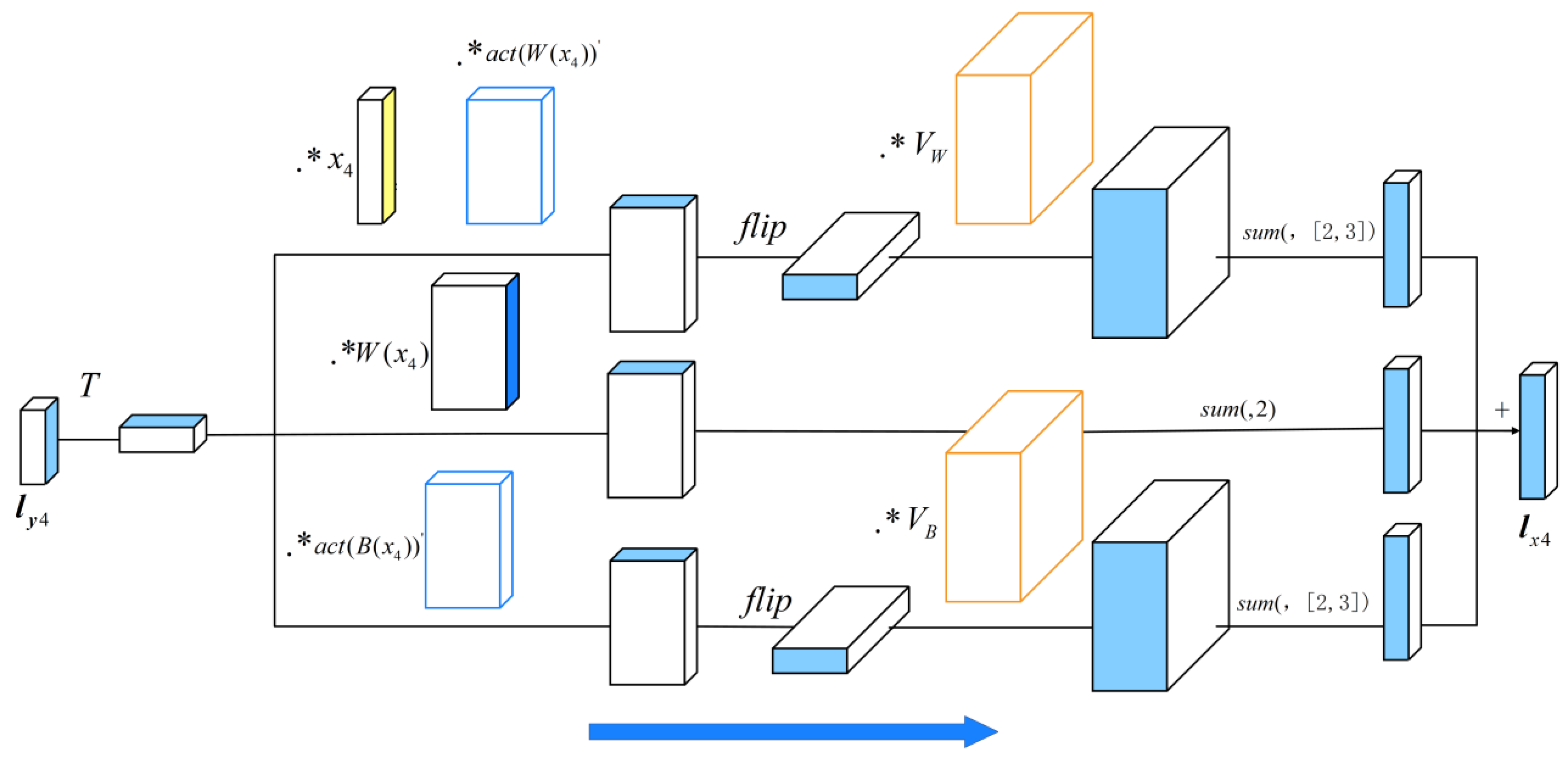
2.1. Core Principle of VWB Net

For the general neural network, the output $y$ is:

$$y=act(w·x+b),$$

(1)

where $x$ is input, $w$ is weight, $b$ is bias, and $act{(}_{})$ is activation function.

For VWB Net, the output $y$ is:

$$y=w(x)·x+b(x),$$

(2)

where variable-weight $w(x)$ is the function of input $x$, and variable-bias $b(x)$ is also the function of input $x$.

For general networks, the input of neurons is a linear combination of input variables, and then output through the activation function, so the ability of nonlinear expression depends on the activation function. The variable-weights and variable-biases of VWB Net are functions of inputs which can automatically adjust the value, integrate the information of each input variable, and improve the nonlinear expression ability of the network. Furthermore, when there is an error between the sensor output and the estimated value at the last node, the variable-bias $b(x)=y-w(x)·x$ is a simpler way to reduce error than adding an unreferenced mapping layer $y=act(w·x+b)$. The VWB Net is specifically designed for the analytical redundancy of the variable cycle engine which is a multi-variable, time-varying, dynamic, and highly nonlinear problem.

The VWB Net has a more powerful capacity for nonlinear expression than general networks which have fixed weights and biases. Take a simple nonlinear function for example:

$$f(x)=x^2+x.$$

(3)

The VWB Net can quickly fit the function as long as $w(x)=x$ and $b(x)=x$.

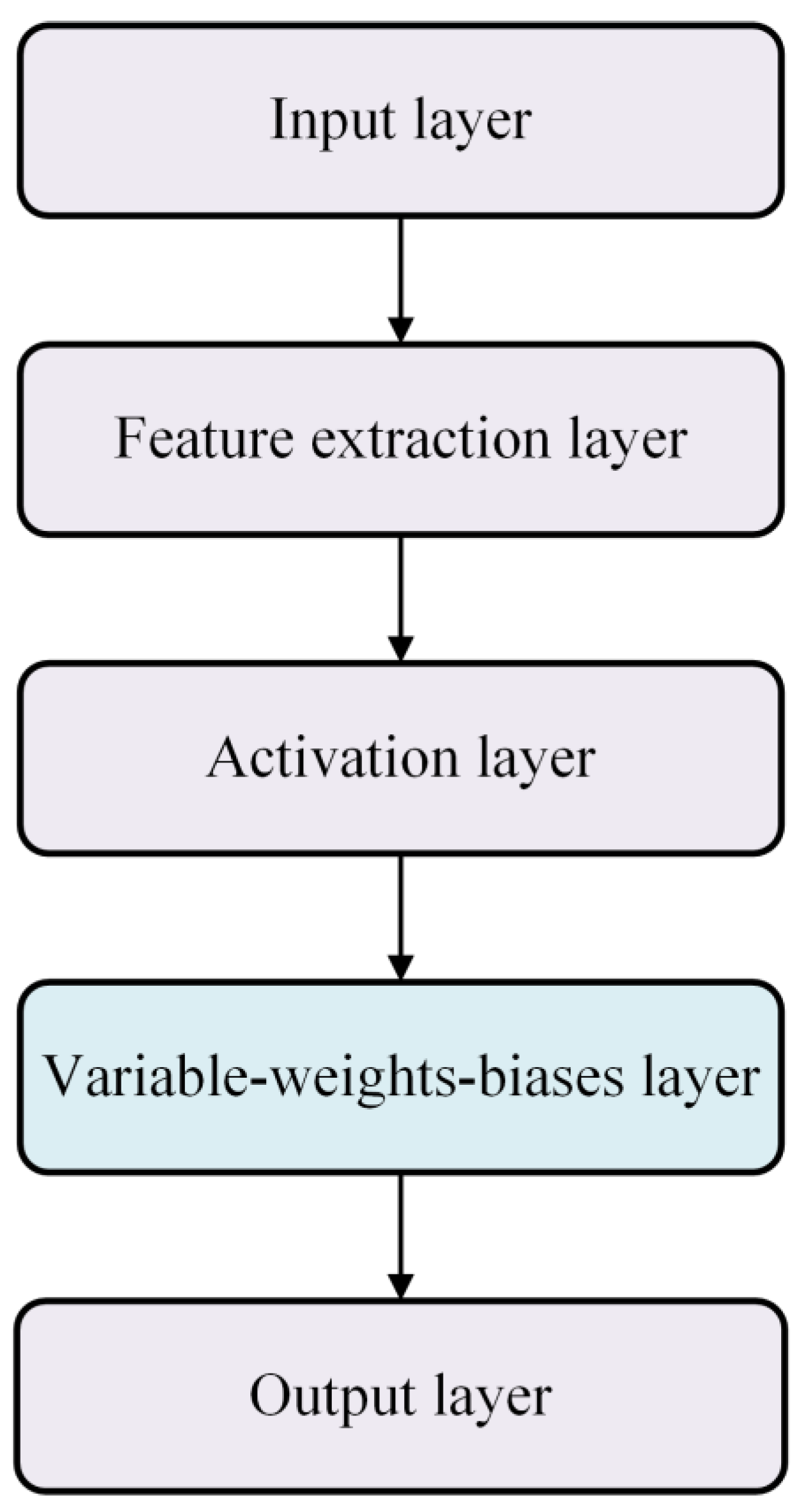
2.2. The Structure of VWB Net

In order to express arrays with different dimensions more clearly, we refer to one-dimensional arrays as vectors, two-dimensional arrays as matrices, and three-dimensional arrays as tensors. The first dimension of all arrays is row, the second dimension is column, and the third dimension is depth.

Operators “$.^$”, “$.*$”, and “$./$” denote operation by element. If the dimensions of two arrays do not match, the lower dimensional array will be copied in the direction of the missing dimension to expand to a higher dimension. For instance,

$$Y=x.*A\iff Y_{i,j}=x_i·A_{i,j},$$

(4)

where $A$ is a matrix of size $(m,n)$, and $x$ is a vector of size $(m,1)$.

In addition, $sum(array,k)$ is the function that sums up the elements of the $kth$ dimension. For instance,

$$sum(X,2)\iff {\displaystyle \sum _{j=1}^n{X}_{i,j}}=x_i,x=[x_1,x_2,\mathrm{\dots },x_m],$$

(5)

where $X$ is a matrix of size $(m,n)$. After $sum(X,2)$, $X$ is transformed into a vector $x$ of size $(m,1)$, $flip{(}_{})$ is referred to as

$$flip(V)\iff V_{k,j,i}=V_{i,j,k},$$

(6)

where $V$ is a tensor of size $(m,n,h)$.

As shown in Figure 1, the VWB Net contains the core layers—the variable-weights-biases layer and auxiliary layers—an input layer, an output layer, and feature extraction layer. Before the formula, it should be noted that in the forward propagation process, the input of each layer is the output of the previous layer. For back propagation, the output loss of each layer is the input loss of the next layer.

Input layer normalizes input data as follows.

$$Y_1=(X_1-\mu )./\sigma ,$$

(7)

where $X_1$ is the input data map of size $(m,n)$, $\mu$ sizing $(m,1)$ is a column vector whose row elements are mean values of each row, and $\sigma$ sizing $(m,1)$ is a column vector whose row elements are standard deviations of each row and no elements equal zero. $Y_1$ is the output data map of size $(m,n)$.

Feature extraction layer is used to refine important feature information by changing the corresponding weights according to the influence of parameters. For example, if a parameter has a greater influence, its weight is greater. Additionally, by the addition of Equation (8), this layer shrinks the number of parameters.

The output of the feature separation layer is.

$$y_2=sum(X_2.*W,2)+b,$$

(8)

where $X_2$ is the data map of size $(m,n)$, $W$ is the weight matrix of size $(m,n)$, $b$ is the bias vector of size $(m,1)$, and $y_2$ is the output vector of size $(m,1)$.

The backward propagation process is defined as follows.

The input loss of the feature extraction layer is defined as

$$L_x{}_2=l_y{}_2.*W.$$

(9)

The weight gradient of the feature extraction layer is

$$D_W{}_2=l_y{}_2.*X_2.$$

(10)

The bias gradient of the feature extraction layer is

$$d_b{}_2=l_y{}_2.$$

(11)

The weight matrix of the feature extraction layer is

$$W=W-{\eta }_2·D_W{}_2.$$

(12)

The bias vector for the feature extraction layer is

$$b=b-{\eta }_2·d_{b2},$$

(13)

where $l_y{}_2$ is the output loss vector of size $(m,1)$, and η₂ is the constant learning rate of the feature extraction layer.

Activation layer uses LeakyReLU as the activation function. Its forward propagation is given as

$$y_3=act(x_3),$$

(14)

$$act(x_3)=\left\{\begin{array}{cc}{x}_3& x_3\ge 0\\ 0.01·x_3& x_3<0\end{array}\right..$$

(15)

Its back propagation is defined as

$$l_x{}_3=\left\{\begin{array}{cc}{l}_y{}_3& x_3\ge 0\\ 0.01·l_y{}_3& x_3<0\end{array}\right.,$$

(16)

where $x_3$ sizing $(m,1)$ is the input data of the activation layer, $l_x{}_3$ sizing $(m,1)$ is the input loss of the activation layer, and $l_y{}_3$ sizing $(m,1)$ is the output loss of the activation layer. LeakyReLU addresses an issue of ReLU, where the derivative is zero when the input is negative which can make it difficult for the model to update during training. The advantage of LeakyReLU for the analytical redundancy problem of variable cycle engines with multiple variables is that it can increase the nonlinear ability of the model, thereby better fitting the analytical relationship.

Variable-weights-biases layer enhances the algorithm’s nonlinear expressive capability by separately making weights and biases functions of inputs. The following equation describes the forward propagation process of the variable-weights-biases layer.

The output vector of the variable-weights-biases layer is given as

$$\begin{array}{ll}{y}_4& =W(x_4)·x_4+B(x_4)\\ & =sum\left(act\right(flip(sum(x_4.*V_W,1))+O_W).*x_4\\ +act\left(flip\right(sum(x_4.*V_B,1))+O_B),1){)}^T\end{array}.$$

(17)

The weights matrix is given as

$$W(x_4)=\left\{\begin{array}{cc}{x}_4·V_W+O_W& (x_4·V_W+O_W)\ge 0\\ 0.01(x_4·V_W+O_W)& (x_4·V_W+O_W)<0\end{array}\right..$$

(18)

Variable-biases matrix is given as

$$B(x_4)=\left\{\begin{array}{cc}{x}_4·V_B+O_B& (x_4·V_B+O_B)\ge 0\\ 0.01(x_4·V_B+O_B)& (x_4·V_B+O_B)<0\end{array}\right.,$$

(19)

where $act{(}_{})$ is the LeakyReLU activation function, $y_4$ is the output vector of size $(n,1)$, $x_4$ is the input vector of size $(m,1)$, $V_W$ is the tensor of variable-weights sizing $(m,n,m)$, $O_W$ is the offset matrix of variable-weights sizing $(m,n)$, $V_B$ is the tensor of variable-biases sizing $(m,n,m)$, and $O_B$ is the offset matrix of variable-biases sizing $(m,n)$.

As shown in Equations (18) and (19), $W(x_4)$ and $B(x_4)$ are functions of input $x_4$.

Furthermore, the variable-biases matrix can be obtained by

$$B(x_4)=y-W(x_4)·x_4.$$

(20)

Variable-biases $B(x_4)$ help the estimated value reach the target value at the last node. For example, if an identity mapping were optimal, it would be simpler to push the variable-biases to zero.

A graphic forward propagation of $x_4$ (Equation (17)) is shown in Figure 2. The expression of the variable-weights-biases layer is $y_4=W(x_4)·x_4+B(x_4)$.

The back propagation process is shown as follows.

The tensor gradient of the variable-weights:

$$\begin{array}{ll}{D}_{V_W}=\frac{\partial l}{\partial V_W}& =\frac{\partial l}{\partial y_4}·\frac{\partial y_4}{\partial W(x_4)}·\frac{\partial W(x_4)}{\partial (V_W·x_4+O_W)}·\frac{\partial (V_W·x_4+O_W)}{\partial V_W}\\ & =l_y{}_4·x_4·{W(x_4)}^{\prime }·x_4\\ & =flip(l_y{{}_4}^T.*x_4.*act({W(x_4))}^{\prime }).*x_4\end{array}.$$

(21)

The offset gradient of the variable-weights:

$$\begin{array}{ll}{D}_{O_W}=\frac{\partial l}{\partial O_W}& =\frac{\partial l}{\partial y_4}·\frac{\partial y_4}{\partial W(x_4)}·\frac{\partial W(x_4)}{\partial (V_B·x_4+O_W)}·\frac{\partial (V_B·x_4+O_W)}{\partial O_W}\\ & =l_y{}_4·x_4·W{(x_4)}^{\prime }\\ & =l_y{{}_4}^T.*x_4.*act{(W(x_4))}^{\prime }\end{array}.$$

(22)

The tensor gradient of the variable-biases:

$$\begin{array}{ll}{D}_{V_B}=\frac{\partial l}{\partial V_B}& =\frac{\partial l}{\partial y_4}·\frac{\partial y_4}{\partial B(x_4)}·\frac{\partial B(x_4)}{\partial (V_B·x_4+O_B)}·\frac{\partial (V_B·x_4+O_B))}{\partial V_B}\\ & =l_y{}_4·B{(x_4)}^{\prime }·x_4\\ & =flip(l_y{{}_4}^T.*act{(B(x_4))}^{\prime }).*x_4\end{array}.$$

(23)

The offset gradient of the variable-biases:

$$\begin{array}{ll}{D}_{O_B}& =\frac{\partial l}{\partial O_B}=\frac{\partial l}{\partial y_4}.\frac{\partial y_4}{\partial B(x_4)}.\frac{\partial B(x_4)}{\partial (V_B·x_4+O_B)}.\frac{\partial (V_B·x_4+O_B)}{\partial O_B}\\ & =l_y{}_4·B{(x_4)}^{\prime }\\ & =l_y{{}_4}^T.*act{(B(x_4))}^{\prime }\end{array}.$$

(24)

The tensor of variable-weights:

$$V_W=V_W-{\eta }_4·D_{V_W}.$$

(25)

The offset matrix of variable-weights:

$$O_W=O_W-{\eta }_4·D_{O_W}.$$

(26)

The tensor of variable-biases:

$$V_B=V_B-{\eta }_4·D_{V_B}.$$

(27)

The offset matrix of variable-biases:

$$O_B=O_B-{\eta }_4·D_{O_B}.$$

(28)

The input loss in variable-weights-biases layer:

$$\begin{array}{l}{l}_x{}_4=\frac{\partial l}{\partial x_4}=\frac{\partial l}{\partial y_4}·\frac{\partial y_4}{\partial W(x_4)}·\frac{\partial W(x_4)}{\partial (V_W ·x_4+O_W)}·\frac{\partial (V_W ·x_4+O_W)}{\partial x_4}\\ +\frac{\partial l}{\partial y_4}·\frac{\partial y_4}{\partial x_4}+\frac{\partial l}{\partial y_4}·\frac{\partial y_4}{\partial B(x_4)}·\frac{\partial B(x_4)}{\partial (V_B ·x_4+O_B)}·\frac{\partial (V_B ·x_4+O_B)}{\partial x_4}\\ = l_y{}_4·x_4·act{(W(x_4))}^{\prime }·V_W+l_y{}_4·W(x_4)+l_y{}_4·act{(B(x_4))}^{\prime }·V_B \\ =sum(flip({l_{y4}}^T.*x_4.*act({W(x_4))}^{\prime }).*V_W,[2,3])\\ +sum(l_y{{}_4}^T.*W(x_4),2)\\ +sum(flip(l_y{{}_4}^T.*act{(B(x_4))}^{\prime }).*V_B,\left[2,3\right])\end{array},$$

(29)

where $l_y{}_4$ is the output loss sizing $(n,1)$. When $sum(tensor,\left[2,3\right])$, a tensor will be transformed into a vector. $sum(tensor,[2,3])$ implies obtaining the summary along a tensor’s second and third dimensions.

A graphic description of back propagation of $l_y{}_4$ (Equation (29)) is presented in Figure 3.

Output layer loss function definition is given as

$$l(y_e)={(y_e-y_a)}^{.^2}./(2·n),$$

(30)

where $y_e$ is the estimated output vector of size $(n,1)$ which is the output data of the variable-weights-biases layer. $y_a$ is the actual output vector of size $(n,1)$.

The loss of the output layer is defined as

$$l_{x5}=(y_e-y_a)./n,$$

(31)

where $l_{x5}$ is the loss of size $(n,1)$.

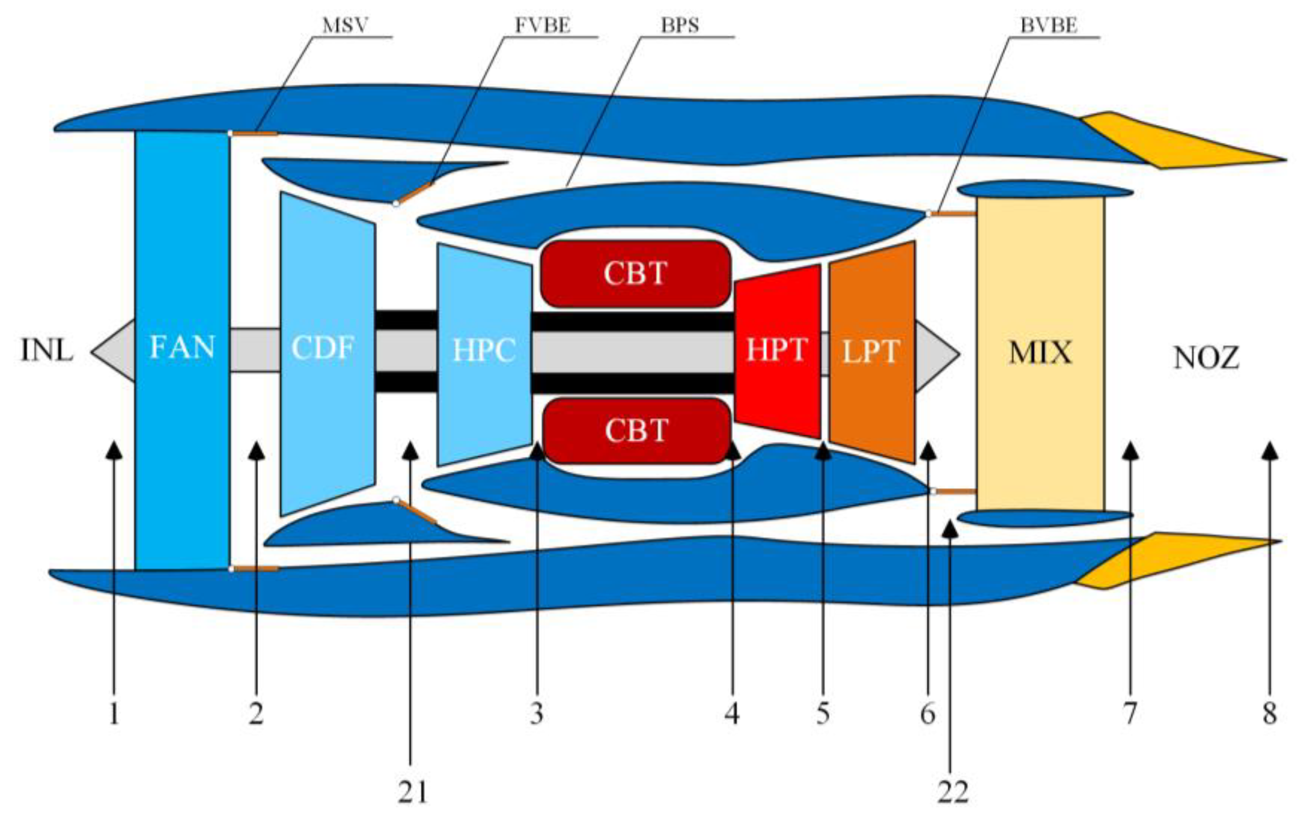
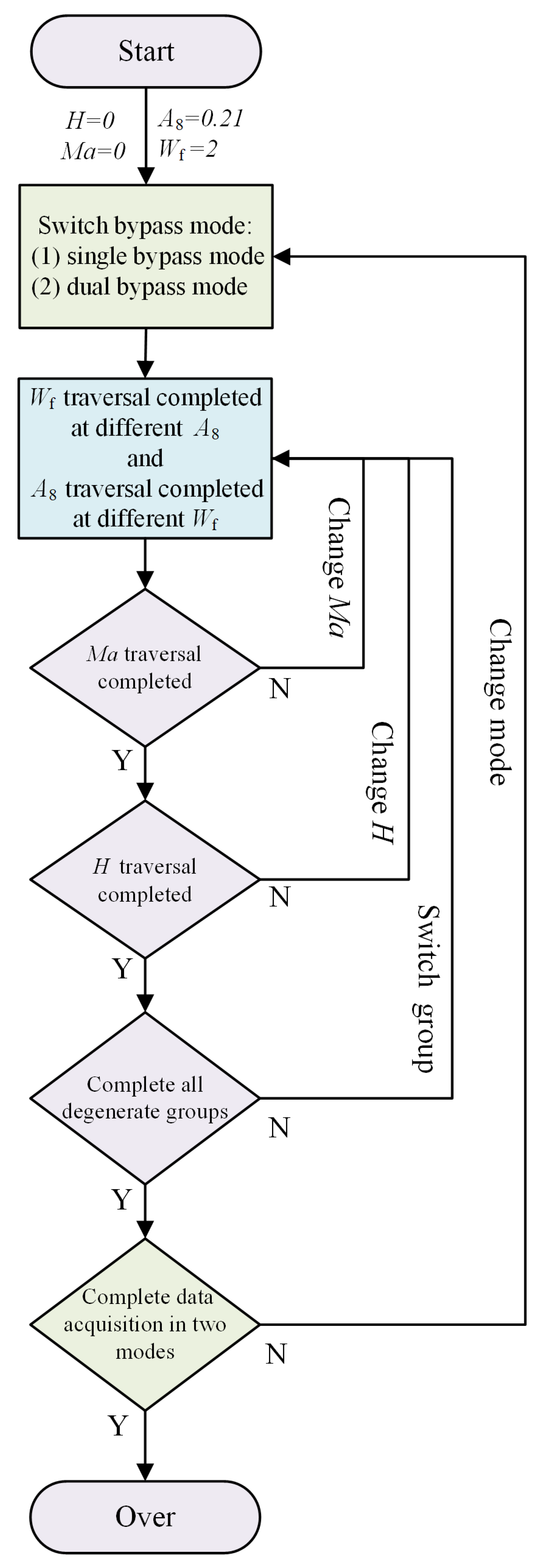
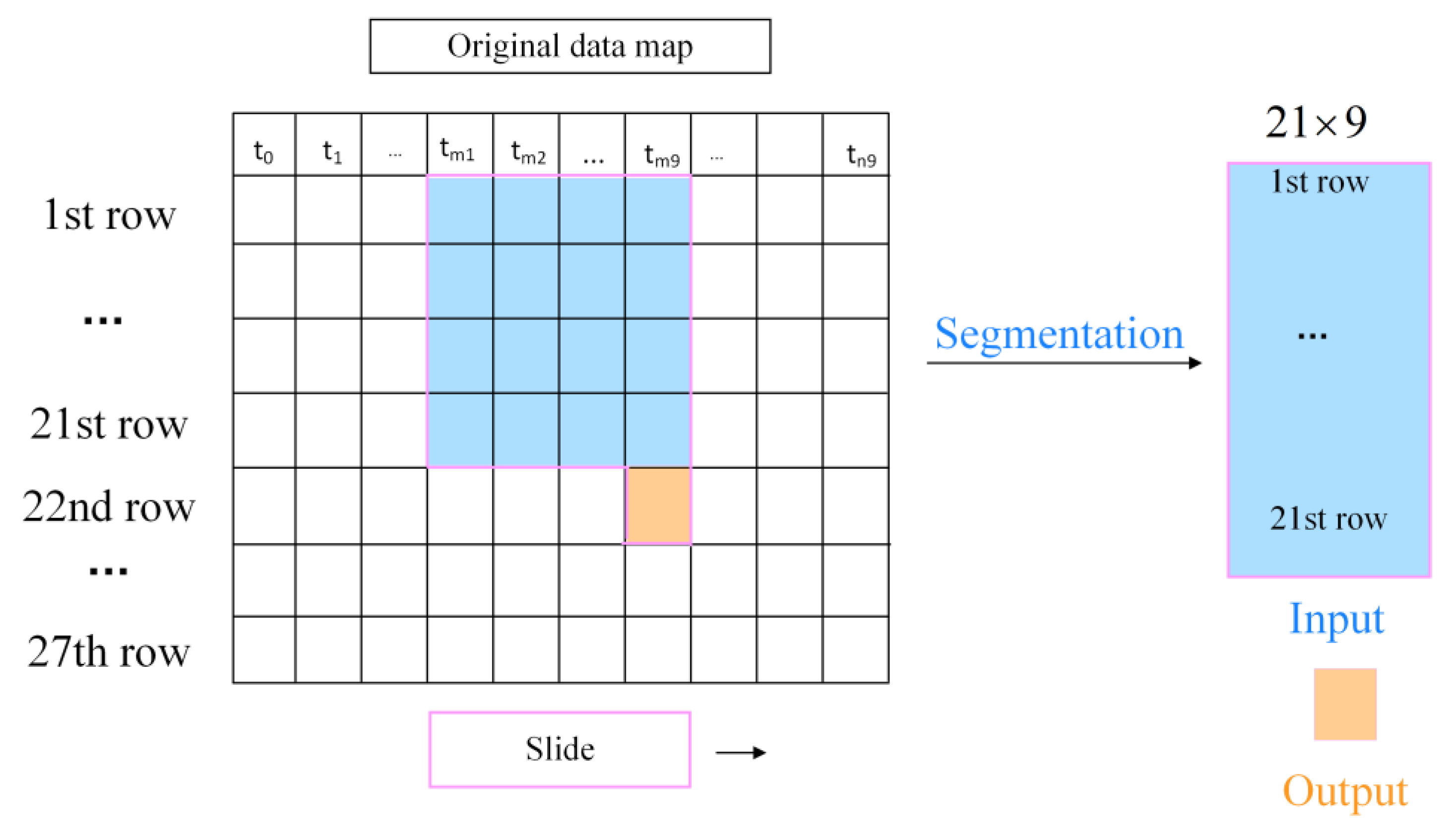
2.3. Data Acquisition of Experiment Object

The basic structure and design point of the variable cycle engine are the same as that in Aygun and Turan’s paper [31]. VCE structure is depicted in Figure 4. Mode Switch Valve (MSV), Forward Variable Bypass Ejector (FVBE), and Back Variable Bypass Ejector (BVBE) are used to control VCE operating modes. Core Driven Fan (CDF), High-Pressure Compressor (HPC), and High-Pressure Turbine (HPT) are coaxial. Fan (FAN) and Low-Pressure Turbine (LPT) are coaxial. Additionally, other major components of VCE include Inlet (INL), Combustion (CBT), Mixer (MIX), Nozzle (NOZ), and Bypass (BPS).

The problem studied in the paper is the analytical redundancy under the degradation condition of VCE. The degradation coefficients are introduced to simulate the performance degradation of engine components. Then, the data of the engine model under different degradation conditions are acquired to train the neural networks.

Degradation coefficients are defined as

$$D_{com,m}=\frac{m_{com,degradation}}{m_{com,nomimal}},$$

(32)

$$D_{com,e}=\frac{e_{com,degradation}}{e_{com,nomimal}},$$

(33)

where $D_{com,m}$ and $D_{com,e}$ represent the degradation coefficients of the mass flow rate and the adiabatic efficiency of each component, respectively. $m_{com,degradation}$ is the mass flow rate of the component after degradation and $m_{com,nominal}$ is the nominal mass flow rate before degradation. $e_{com,degradation}$ is the adiabatic efficiency of the component after degradation and $e_{com,nomimal}$ is the nominal adiabatic efficiency before degradation.

In this study, ten degradation coefficients act on variable cycle engine simultaneously $D_{fan,m}$, $D_{fan,\mathrm{e}}$, $D_{cdf,m}$, $D_{cdf,\mathrm{e}}$, $D_{hpc,m}$, $D_{hpc,\mathrm{e}}$, $D_{hpt,m}$, $D_{hpt,\mathrm{e}}$, $D_{lpt,m}$, and $D_{lpt,\mathrm{e}}$. The 10 degradation coefficients are random values within 0.96–1 and a total of 20 sets of degradation combinations are set randomly. The data acquisition is carried out under the 20 combinations.

Table 1. Explanation of symbols in original data set.

Row	Symbol	Explanation	Unit	Range
1	$H$	Flight height	km	0–12
2	$Ma$	Flight Mach number		0–2
3	$W_{\mathrm{f}}$	Fuel consumption	kg/s	2–2.8
4	$A_8$	Nozzle area	m2	0.21–0.25
5	$M_{\mathrm{sv},\mathrm{ope}}$	The opening of MSV		[0, 100]
6	$F_{\mathrm{vbe},\mathrm{ope}}$	Opening of forward variable bypass ejector		[0, 100]
7	$B_{\mathrm{vbe},\mathrm{ope}}$	Opening of backward variable bypass ejector		[0, 100]
8	$T_1$	Fan inlet total temperature	K
9	$P_1$	Fan inlet total pressure	Pa
10	$T_2$	Core driven fan inlet total temperature	K
11	$P_2$	Core driven fan inlet total pressure	Pa
12	$T_{21}$	High-pressure compressor inlet total temperature	K
13	$P_{21}$	High-pressure compressor inlet total pressure	Pa
14	$T_{22}$	Bypass outlet total temperature	K
15	$P_{22}$	Bypass outlet total pressure	Pa
16	$T_7$	Mixer outlet total temperature	K
17	$P_7$	Mixer outlet total pressure	Pa
18	$T_8$	Nozzle outlet total temperature	K
19	$P_8$	Nozzle outlet total pressure	Pa
20	$P_5$	High-pressure turbine outlet total pressure	Pa
21	$T_6$	Low-pressure turbine outlet total temperature	K
22	$N_l$	Low-pressure rotor speed	r/min
23	$N_h$	High-pressure rotor speed	r/min
24	$P_3$	High-pressure compressor outlet total pressure	Pa
25	$T_5$	High-pressure turbine outlet total temperature	K
26	$P_6$	Low-pressure turbine outlet total pressure	Pa
27	$EPR$	Engine pressure ratio

lists all variables. The original data acquired include two environmental variables ($H$ and $Ma$), five input control variables ($W_{\mathrm{f}}$, $A_8$, $M_{\mathrm{sv},\mathrm{ope}}$, $F_{\mathrm{vbe},\mathrm{ope}}$, and $B_{\mathrm{vbe},\mathrm{ope}}$), and twenty measurable variables ($T_1$, $P_1$, $T_2$, $P_2$, $T_{21}$, $P_{21}$, $T_{22}$, $P_{22}$, $T_7$, $P_7$, $T_8$, $P_8$, $P_5$, $T_6$, $N_l$, $N_h$, $P_3$, $T_5$, $P_6$, and $EPR$) during the operation of variable cycle engine. In order to verify the proposed method, we use the variables from rows 1 to 21 as input, take three typical signals’ estimation ($N_l$, $P_3$, and $T_5$) as output in the digital simulation experiment, and take two typical signals’ estimation ($N_l$ and $EPR$) as output in the HIL simulation experiment. To validate the fundamental feasibility of the proposed method, the effects of Cdf stator angle, Hpc stator angle, and turbine guide vane angle have been neglected to simplify the problem. However, these factors will be investigated in future studies.

The engine model and the analytical redundancy model in digital simulation are both constructed in MATLAB R2021b. In hardware in the loop simulation, the analytical redundancy model and PID controller are built in CodeWarrior 10.5.1. In order to acquire the engine data of dynamic operation and steady operation with performance degradation, under single bypass and dual bypass engine modes across a large envelope, we acquire the simulation data from the component-level model of VCE according to Figure 5. The VCE operates in single bypass and dual bypass modes, respectively. In the process of traversing the fuel consumption $W_{\mathrm{f}}$, make $W_{\mathrm{f}}$ step up in a randomly selected amplitude among {0.05 kg/s, 0.1 kg/s, and 0.2 kg/s} and continue to step up randomly after 1.5 s of steady-state operation. After rising to the upper limit, make $W_{\mathrm{f}}$ step down in a randomly selected amplitude among {0.05 kg/s, 0.1 kg/s, and 0.2 kg/s} and continue to step down after 1.5 s of steady-state operation. The process of traversing $W_{\mathrm{f}}$ is completed when the object reaches the bottom limit. During each $W_{\mathrm{f}}$ traversal, $A_8$ maintains a fixed value. The nozzle area $A_8$ is varied in 0.1 units from 0.21 to 0.25 m². The process described above is repeated for each value of $A_8$, and the $W_{\mathrm{f}}$ traversal is completed again.

Moreover, in the process of traversing the nozzle area $A_8$, make $A_8$ step up in a randomly selected amplitude among {0.05 m², 0.1 m², and 0.2 m²} and continue to step up randomly after 1.5 s of steady-state operation. After rising to the upper limit, make $A_8$ step down in a randomly selected amplitude among {0.05 m², 0.1 m², and 0.2 m²} and continue to step down after 1.5 s of steady-state operation. The process of traversing $A_8$ is completed when the object reaches the bottom limit. During each $A_8$ traversal, $W_{\mathrm{f}}$ maintains a fixed value. The fuel consumption $W_{\mathrm{f}}$ is varied in 0.1 units from 0.2 to 0.28 kg/s. The process described above is repeated for each value of $W_{\mathrm{f}}$, and the $A_8$ traversal is completed again.

Due to the random amplitude steps, the above $W_{\mathrm{f}}$ and $A_8$ traversal scheme allows the acquired data to contain both dynamic data and steady-state data at different $W_{\mathrm{f}}$, $A_8$, and change rates. The $W_{\mathrm{f}}$ and $A_8$ traversal process is repeated, followed by the Mach number $Ma$ varied in 0.1 units from 0 to 2, the altitude $H$ increased in 0.5 units from 0 to 12 km, and different degradation parameters.

The acquired data are processed as follows. Variables in the same rows in Figure 6 are the same as those in Table 1. The original input data map is produced using rows 1–21 of data, and the original output array is produced using one of the rows from 22 to 27. Data at different times in different columns, and the data acquired is continuous. Each input data map has nine times of data. $t_{m9}$ is the current moment of the input data map and $t_{m1}$ is the initial moment of the input data map. The two-dimensional input data map set and the corresponding output data set are produced by using sliding segmentation in the original data map as shown in Figure 6. Sliding windows are set for sliding segmentation of the original input data map and the original output array with sliding window dimensions of 21 × 9 and 1 × 1, respectively, and the sliding window is moved in steps of one along the time dimension each time. The data within the sliding window sizing 21 × 9 is selected as the 2D input data map. The data at $t_{m9}$ within the sliding window sizing 1 × 1 is selected as the output data of the two-dimensional input data map. In the same way, the input maps and the output arrays can be obtained. The output arrays of $N_l$, $N_h$, $P_3$, $T_5$, $P_6$, and $EPR$ share the same input data maps. When training VWB Net, BPNN, and Dense net, we only need to change the output array, for example, altering $N_l$ with $P_3$.

3. Experiment, Results, and Discussion

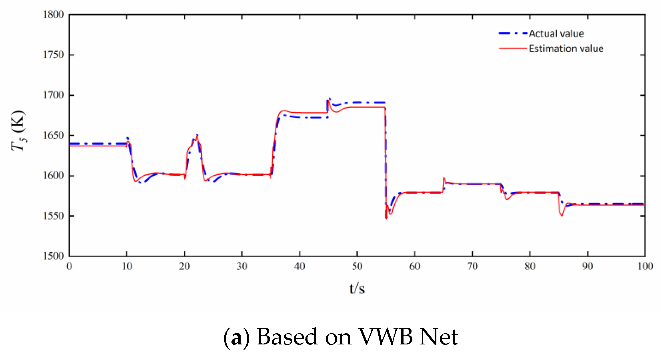
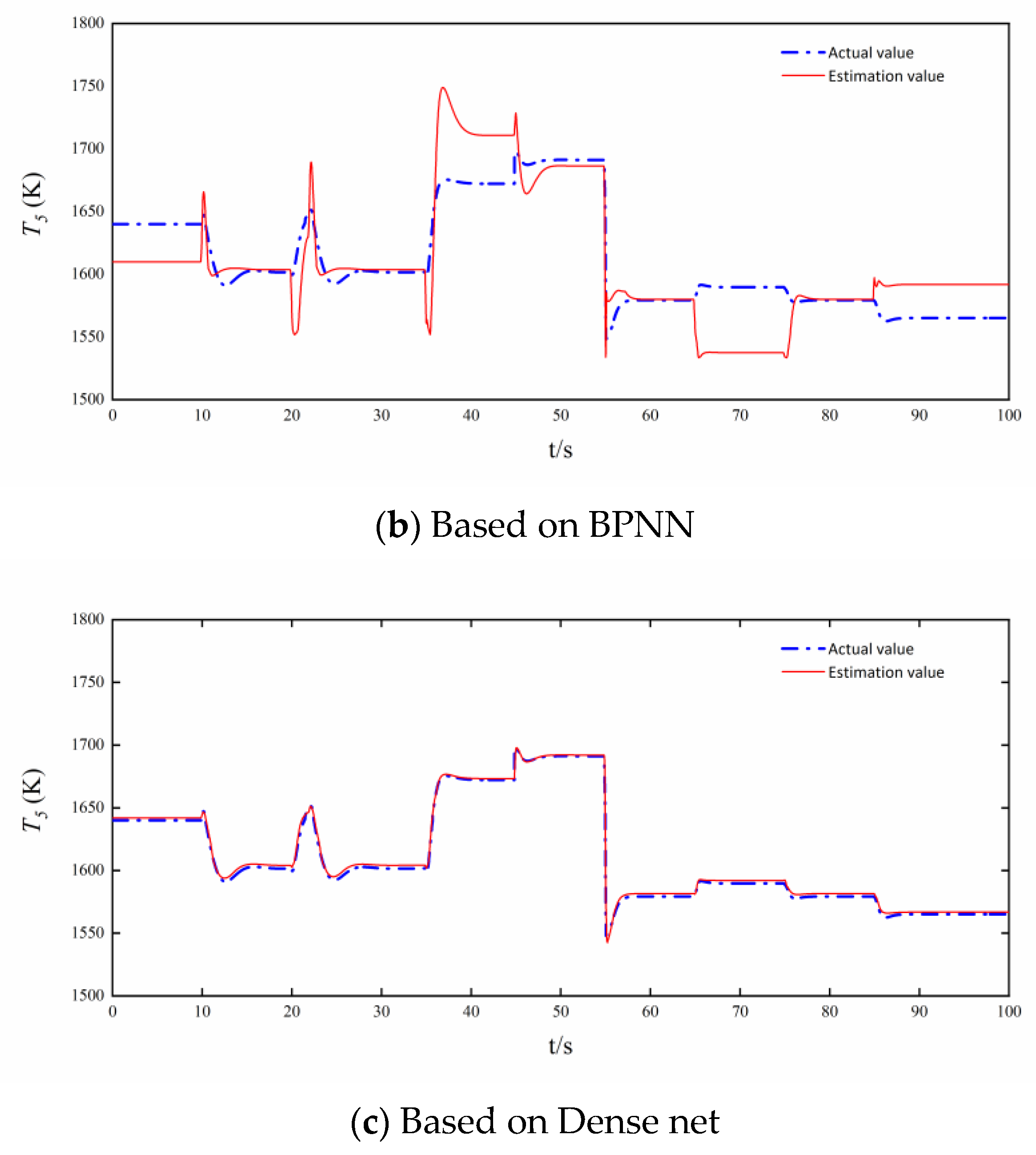
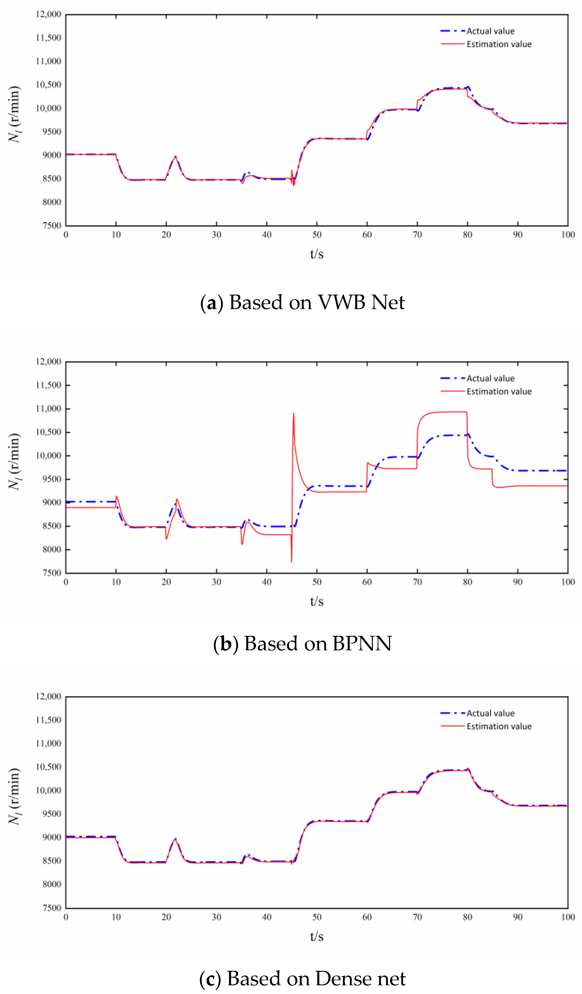
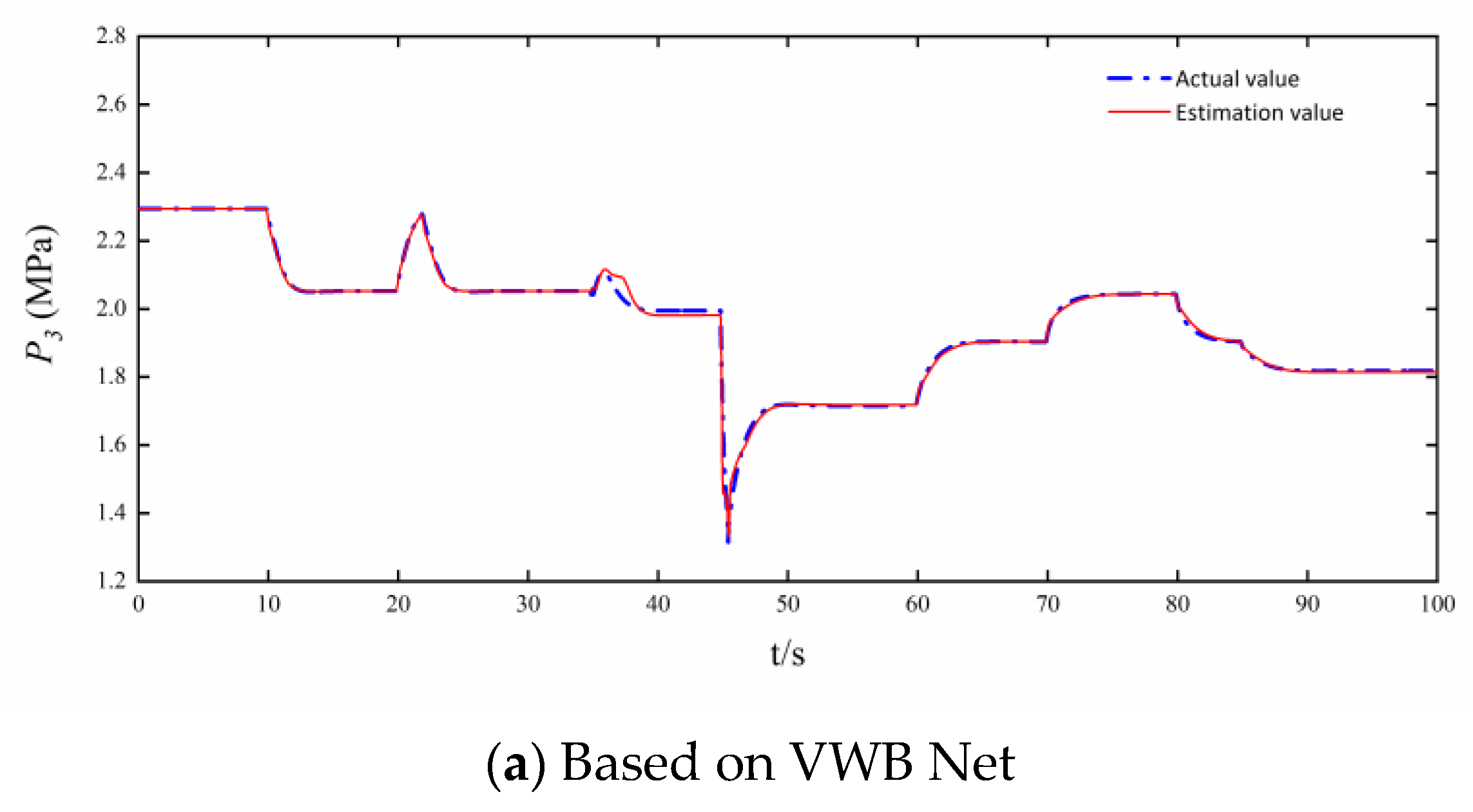
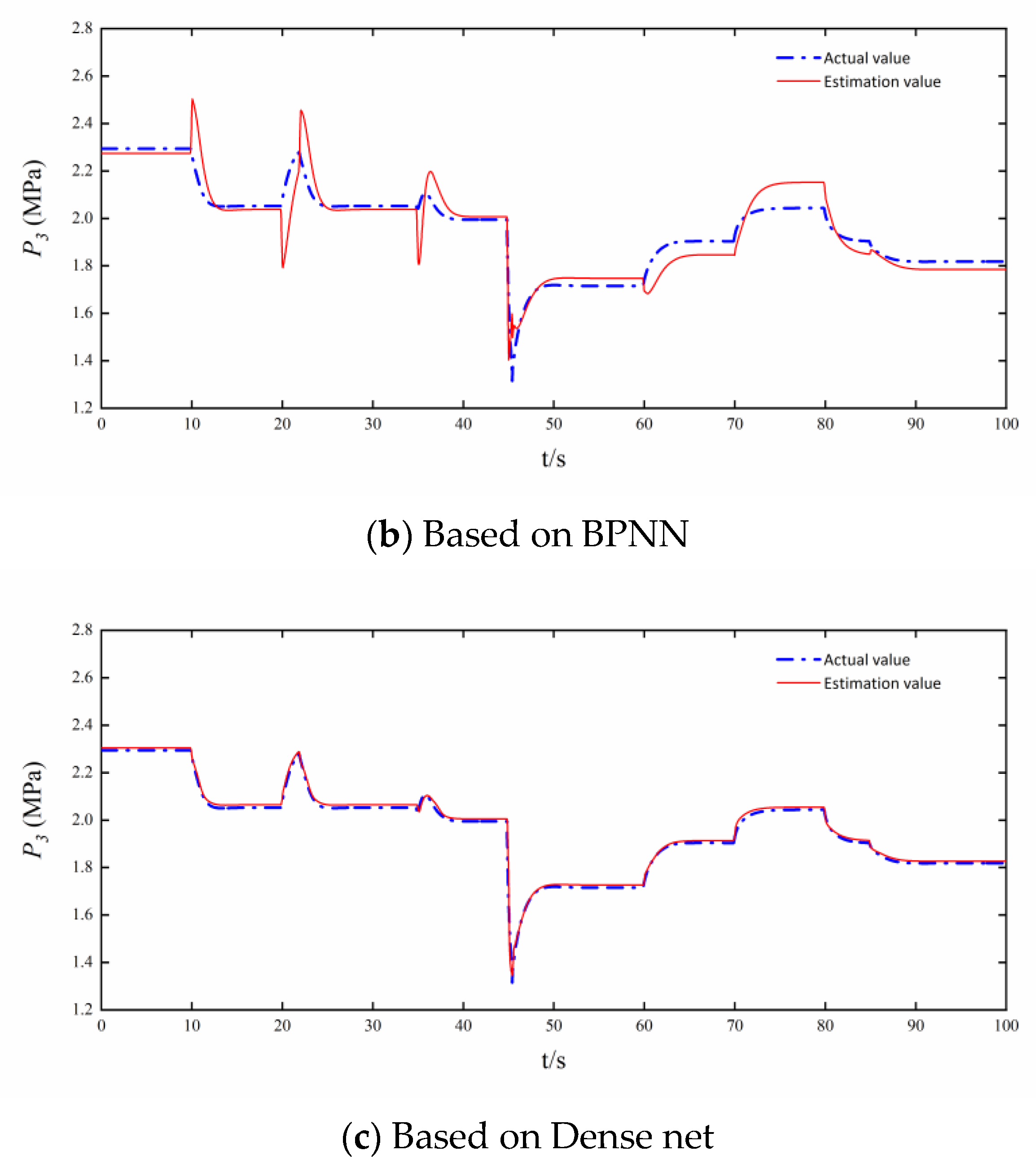
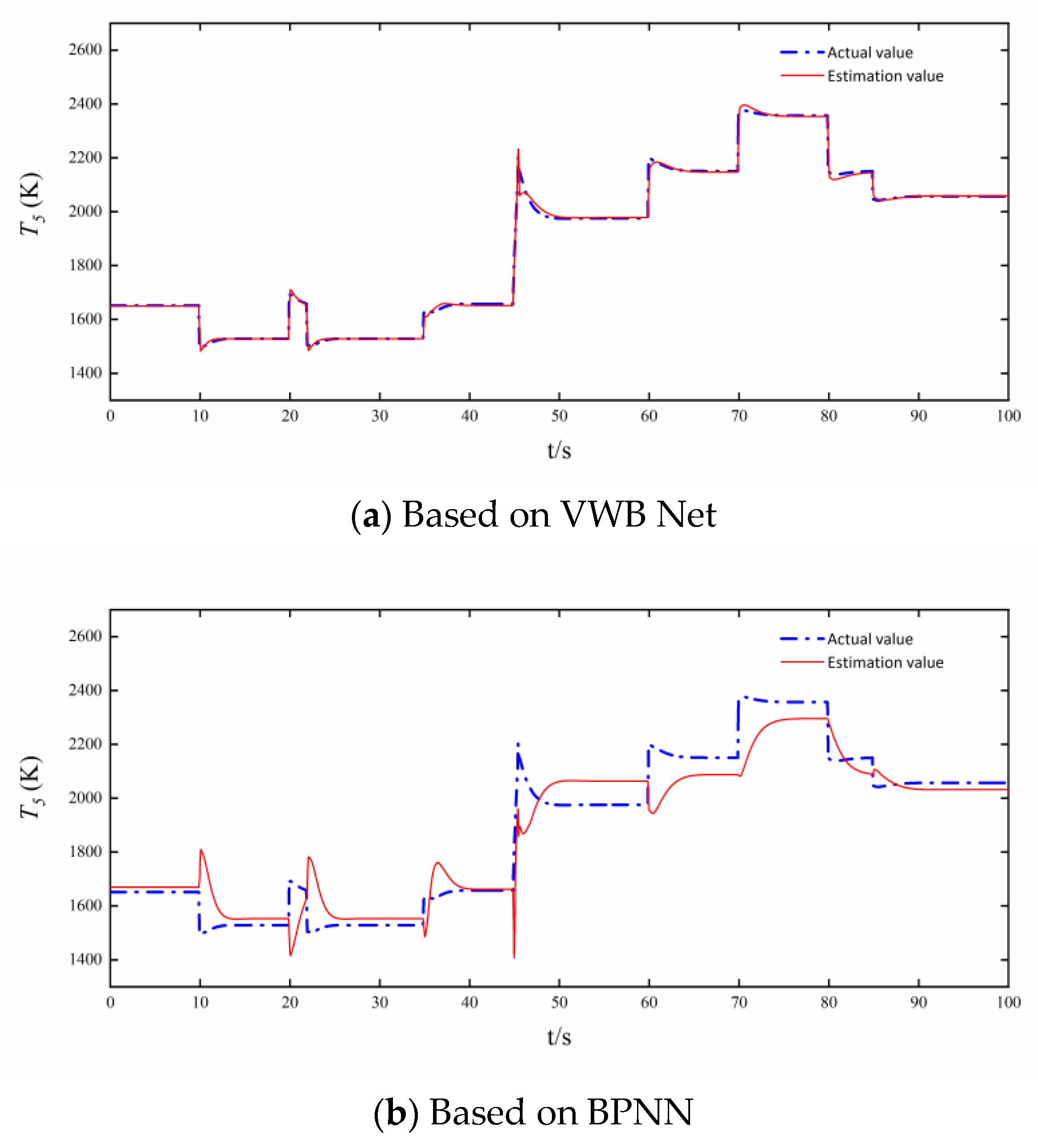
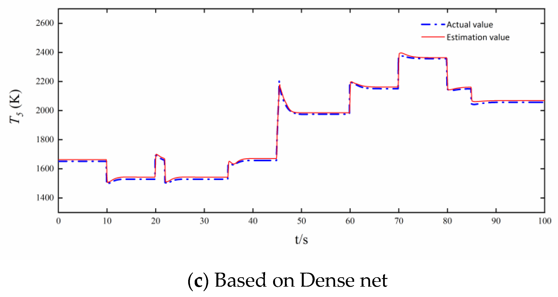
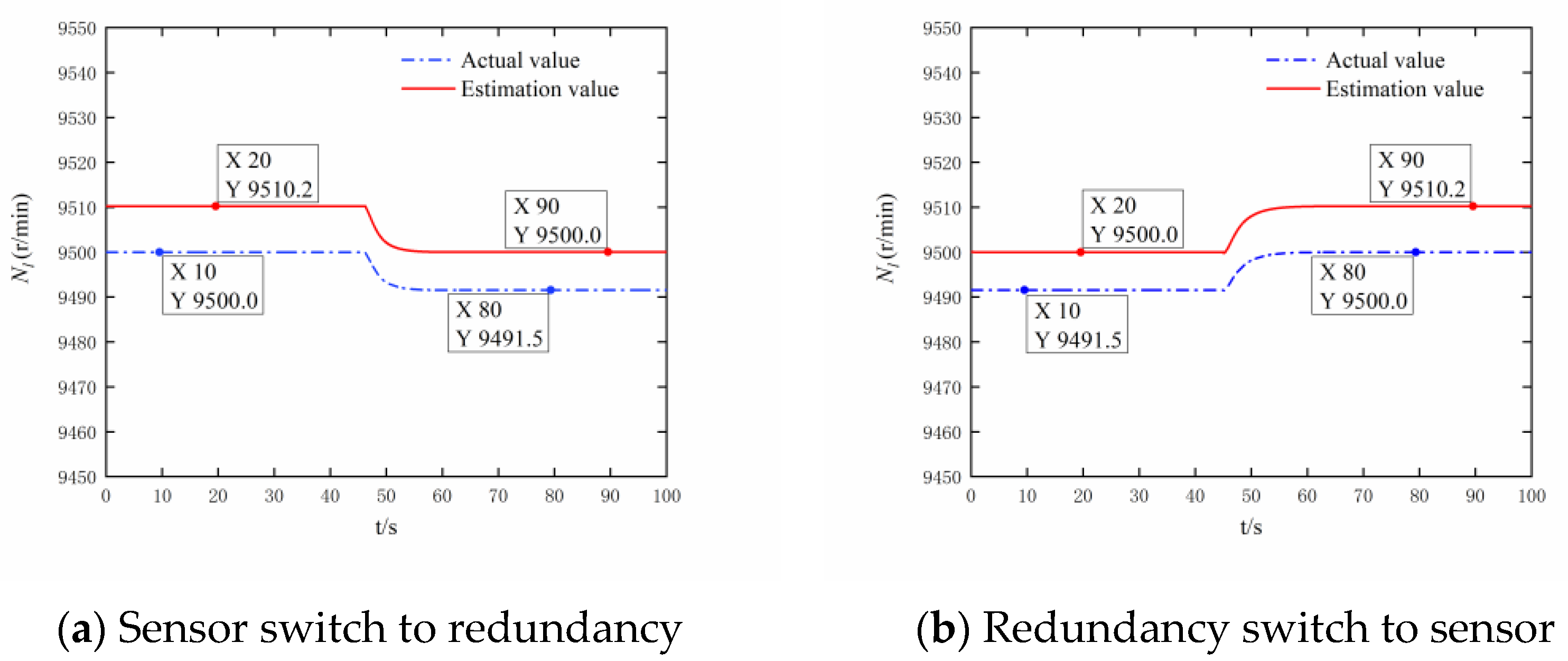
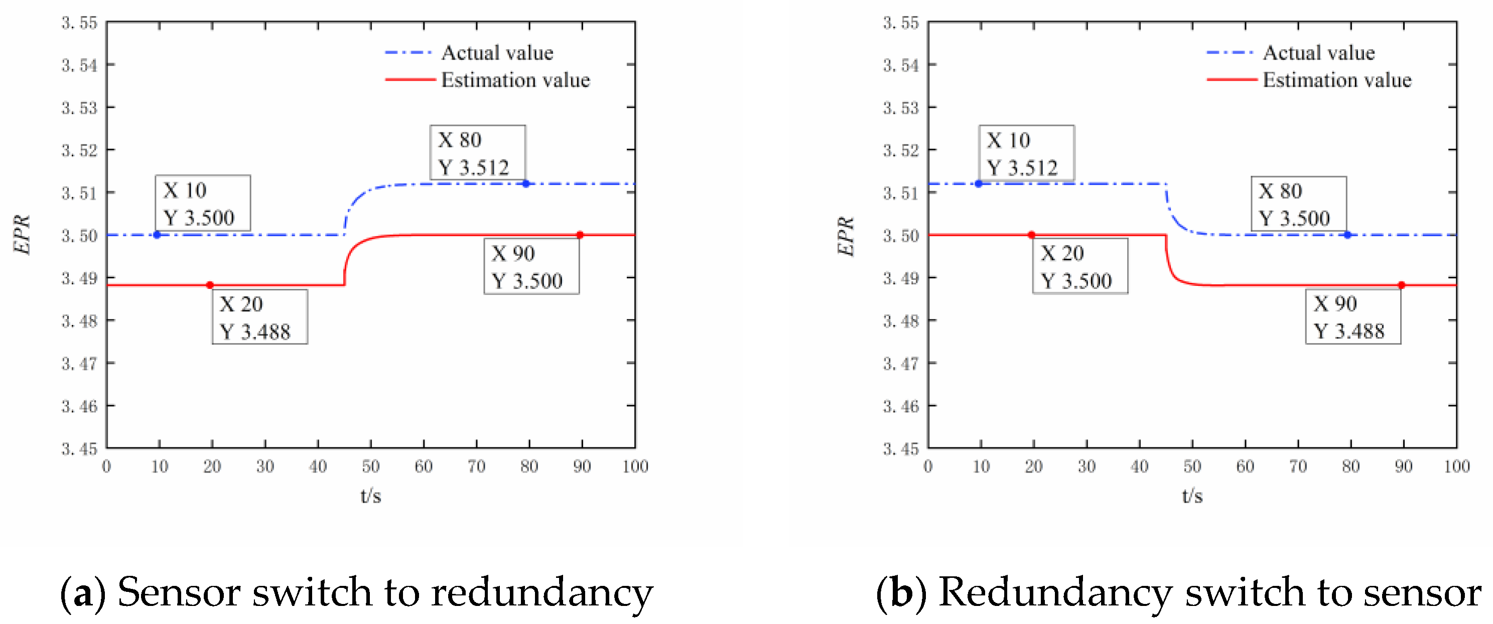
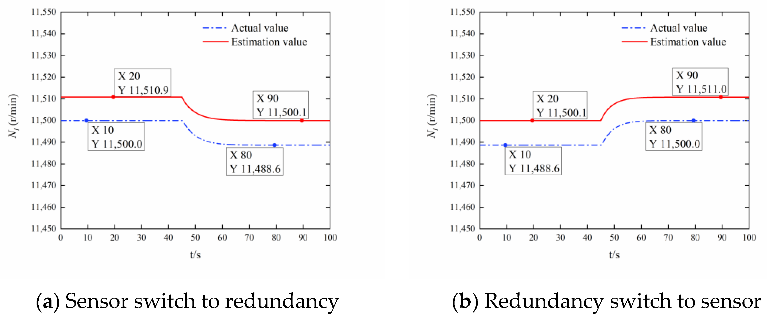
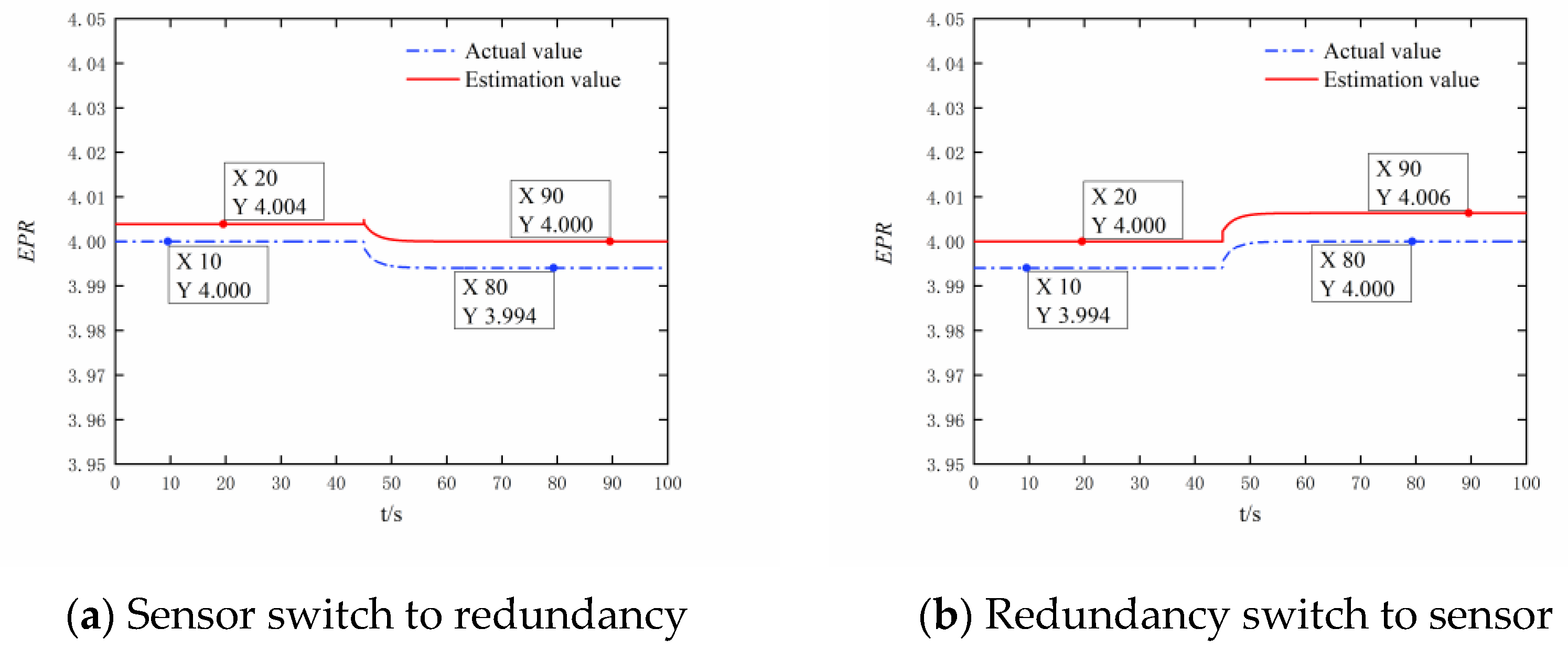
3.1. Digital Simulation Experiment

In the digital simulation, we take the parameter estimation of $N_l$, $P_3$, and $T_5$ as examples to compare the estimation accuracy and real-time performance of VWB Net, BPNN, and Dense net [28]. In order to verify the steady and dynamic performance of VWB Net, the large envelope simulation is conducted in the single and double bypass mode of the variable cycle engine. BPNN is one of the most widely used neural networks. In this paper, BPNN has only five layers which is a typical shallow learning network, and its calculation speed is pretty quick. A Dense net has 709 layers. It is mainly used for high precision, sacrificing a certain computing speed to pursue excellent nonlinear expressive capability.

The variable cycle engine is replaced by a component-level model. Since the control command changes with the flight altitude, Mach number, fuel consumption, and degradation coefficient, the change of the operating point is reflected by the change of the above variables in the simulation. The aircraft climb time is shortened to describe a larger envelope range which is equivalent to increasing the intensity of external interference. If the control system can achieve good results under this condition, the actual performance will be better. Next, the simulation results under single and dual bypass modes are given.

(1)

Single bypass mode simulation validation

The simulation under the single bypass mode starts from the high-altitude design point ($H$ = 12 km, $Ma$ = 1.5). The fuel consumption $W_{\mathrm{f}}$ is 2.4 kg/s. The nozzle area $A_8$ first rises from 0.24 m² to 0.25 m² at the 10th s, then drops to 0.24 m² at the 20th s before quickly rising to 0.25 m² once again. At the 35th s, the nozzle area $A_8$ was reduced to 0.23 m². The engine performance degradation occurs at 45th s. Change the altitude $H$ and the Mach number $Ma$ at the 55th s, so that the engine operates to the operating point of $H$ = 7 km and $Ma$ = 1.2. At the 65th s, the nozzle area $A_8$ falls from 0.23 m² to 0.22 m², then rises to 0.23 m² and 0.24 m² successively. The actual values of speed, temperature, and pressure, and the analytical redundancy of speed, temperature, and pressure based on the three networks in single bypass mode are shown in Figure 7, Figure 8 and Figure 9.

(2)

Dual bypass mode simulation verification

The component-level model of a variable cycle engine in dual bypass mode has a large dynamic process from the ground design point ($H$ = 0 km, $Ma$ = 0). The nozzle area $A_8$ is 0.22 m². The fuel consumption $W_{\mathrm{f}}$ decreases from 2.4 kg/s to 2.0 kg/s at the 10th s, increases from 2.0 kg/s to 2.4 kg/s at the 20th s, and then rapidly decreases to 2.0 kg/s. The engine performance degradation occurs at 35th s. Change the altitude $H$ and the Mach number $Ma$ at the 45th s, so that the variable cycle engine runs to the high-altitude point ($H$ = 11 km, $Ma$ = 1.2). The fuel consumption $W_{\mathrm{f}}$ increases from 2.0 kg/s to 2.4 kg/s at the 60th s, increases to the maximum fuel consumption $W_{\mathrm{f}}$ of 2.8 kg/s at the 70th s, and then decreases to 2.4 kg/s and 2.2 kg/s in turn. The actual values of engine speed, temperature, and pressure, and the analytical redundancy of speed, temperature, and pressure based on the three networks in dual bypass mode are shown in Figure 10, Figure 11 and Figure 12.

Figure 7, Figure 8, Figure 9, Figure 10, Figure 11 and Figure 12 show the steady and dynamic performance of $N_l$, $P_3$, and $T_5$ analytical redundancies based on VWB Net, BPNN, and Dense net. The analytical redundancies based on BPNN are not ideal, and the error of BPNN is far greater than the other two networks. BPNN cannot accurately estimate the dynamic process after the control variable changes instantaneously, and BPNN is the worst in $T_5$ analytical redundancy in Figure 9 and Figure 12. The error of the Dense net is relatively small, and the simulation curve of the Dense net is smoother than that of VWB Net. It is obvious that the VWB Net meets the requirement of the variable cycle engine for prediction accuracy.

The intricacy of the mapping from input to output as well as each net’s nonlinear expressive capabilities can explain differences in the steady and dynamic performance among $N_l$, $P_3$, and $T_5$ based on VWB Net, BPNN, and Dense net.

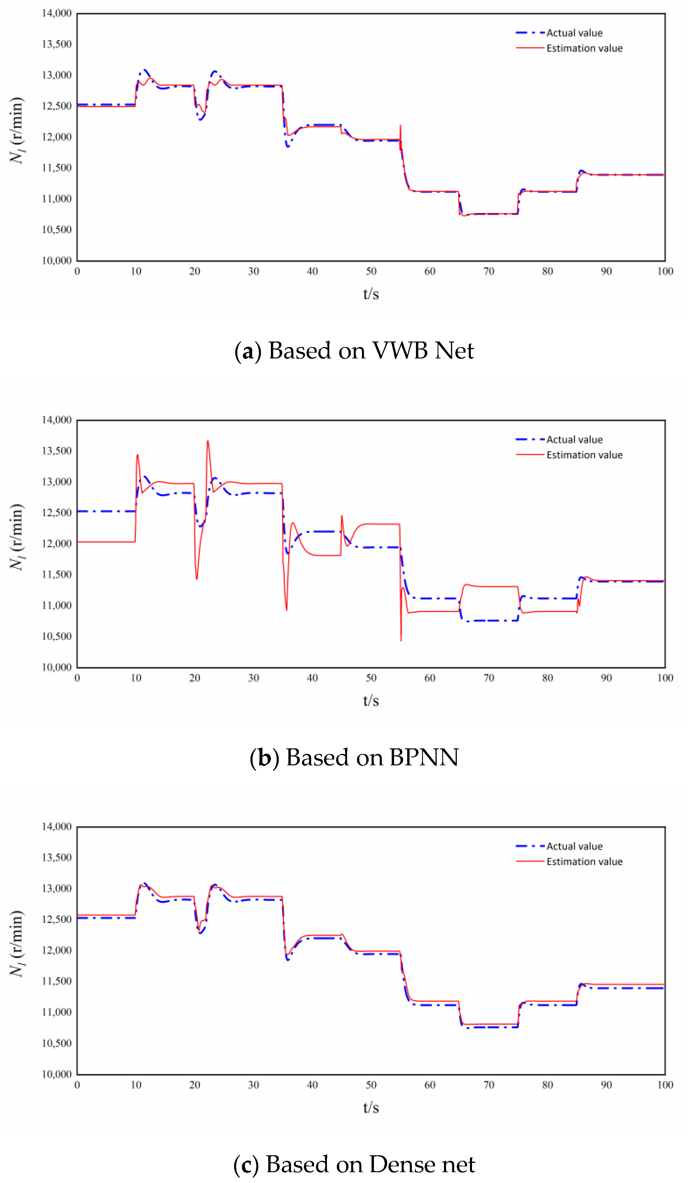
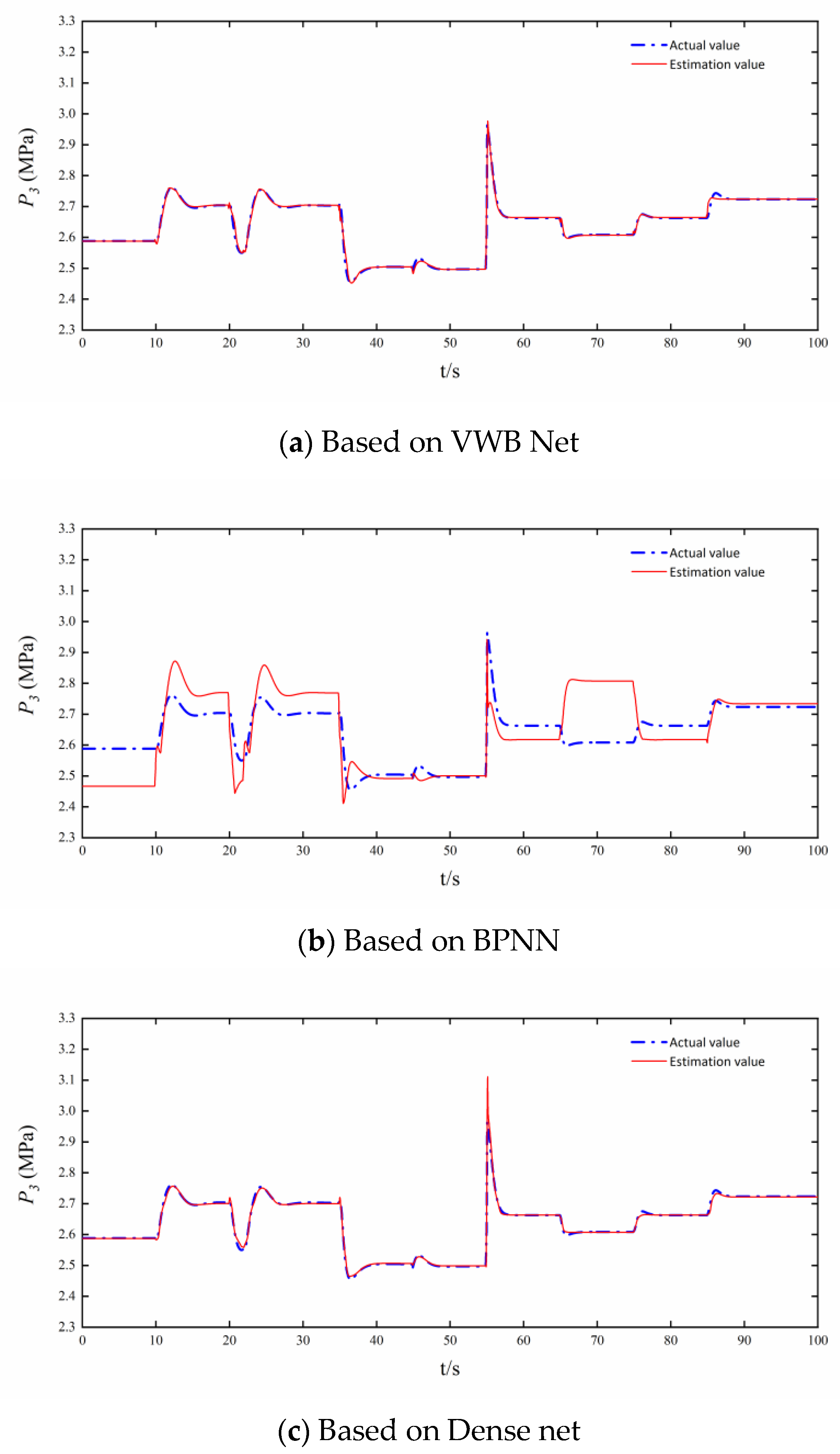
3.2. Comparison of Estimation Accuracy and Real-Time Performance

Based on Section 3.1, the performance of analytical redundancy based on each network is further discussed. VWB Net, BPNN, and Dense net are trained for 12 epochs with a batch size of 50.

Table 2. Number of parameters, number of layers, and calculation speed of VWB Net, BPNN, and Dense net.

Net	${\mathit{P}}_{\mathit{n}}$	${\mathit{L}}_{\mathit{n}}$	${\mathit{S}}_{\mathit{c}}\left(\mathbf{ms}\right)$
VWB Net	65,772	5	1
BPNN	97,664	5	2
Dense net	18,154,753	709	165

shows the number of network parameters ($P_n$), the number of network layers ($L_n$), and the calculation speed of each forward propagation ($S_c$). The calculation speeds of each forward propagation ($S_c$) based on VWB Net and BPNN are less than 2 ms. Obviously, VWB Net and BPNN, except for Dense net, meet the requirement of a variable cycle engine for calculation speed. Compared with the most complex network Dense net, the three indicators of VWB Net and BPNN are tens or even hundreds of times lower than Dense net.

Table 3. Average relative error of $N_l$, $P_3$, and $T_5$ analytical redundancies.

Net	$\mathit{A}\mathit{R}\mathit{E} (\%)$
	${\mathit{N}}_{\mathit{l}}$	${\mathit{P}}_3$	${\mathit{T}}_5$
VWB Net	0.19	0.25	0.27
BPNN	2.65	2.37	3.34
Dense net	0.20	0.34	0.39

and

Table 4. Calculation efficiency and parameter efficiency of $N_l$, $P_3$, and $T_5$ analytical redundancies.

Net	${\mathit{E}}_{\mathit{c}} \mathbf{(}\%/\mathbf{ms}\mathbf{)}$			${\mathit{E}}_{\mathit{p}} \mathbf{(}\%\times {10}^{-5}/\mathbf{parameter}\mathbf{)}$
	${\mathit{N}}_{\mathit{l}}$	${\mathit{P}}_3$	${\mathit{T}}_5$	${\mathit{N}}_{\mathit{l}}$	${\mathit{P}}_3$	${\mathit{T}}_5$
VWB Net	99.81	99.75	99.73	151.75	151.66	151.63
BPNN	48.68	48.82	48.33	99.68	99.97	98.97
Dense net	0.60	0.60	0.60	0.55	0.55	0.55

show the average relative error, calculation efficiency, and parameter efficiency of the analytical redundancies based on VWB Net, BPNN, and Dense net. Calculation efficiency is used to evaluate the accuracy that a network can achieve per millisecond. Furthermore, parameter efficiency is used to evaluate the accuracy that a network can achieve per parameter.

Average relative error is defined as

$$ARE=\frac{{\displaystyle \sum _{i=1}^n\left|A{V}_i-E{V}_i\right|}}{{\displaystyle \sum _{i=1}^{n}A{V}_i}},$$

(34)

where $A{V}_i$ stands for the $ith$ actual value, and $E{V}_i$ is the $ith$ estimation value. $n$ is the number of test data.

Calculation efficiency is defined as

$$E_c=\frac{(1-ARE)}{S_c}.$$

(35)

Parameter efficiency is defined as

$$E_p=\frac{(1-ARE)}{P_n}.$$

(36)

Dense net performs well in the estimation of the analytical redundancies for $N_l$, $P_3$, and $T_5$ which demonstrates the effectiveness of complex topologies in enhancing nonlinear expressive capability. Although the average relative error of $N_l$ based on Dense net is only 0.20%, it comes at the cost of a large number of parameters and 165 ms of computational overhead. BPNN has the lowest accuracy because its ability to mine feature information is weak.

VWB Net excels in average relative errors of $N_l$, $P_3$, and $T_5$. The average relative errors of $N_l$, $P_3$, and $T_5$ based on VWB Net are no more than 0.27%. VWB Net’s calculation efficiency is more than 166 times higher than Dense net’s which shows that VWB Net consumes less calculation time to achieve high accuracy of VCE parameter estimation. Dividing the VWB Net’s parameter efficiency by Dense Net’s parameter efficiency yields a value greater than 276 which shows that the VWB Net consumes fewer parameters to achieve high accuracy of VCE parameter estimation. It can be seen that the VWB Net algorithm plays an important role in improving the ability of mining feature information and reducing network parameters and layers.

The VWB Net can be utilized to build analytical redundancy for the variable cycle engines due to its exceptional estimation accuracy and real-time performance. With the appropriate design of network parameters and structure, variable-weights and variable-biases can be added to all kinds of networks to achieve higher estimation accuracy and faster calculation speed.

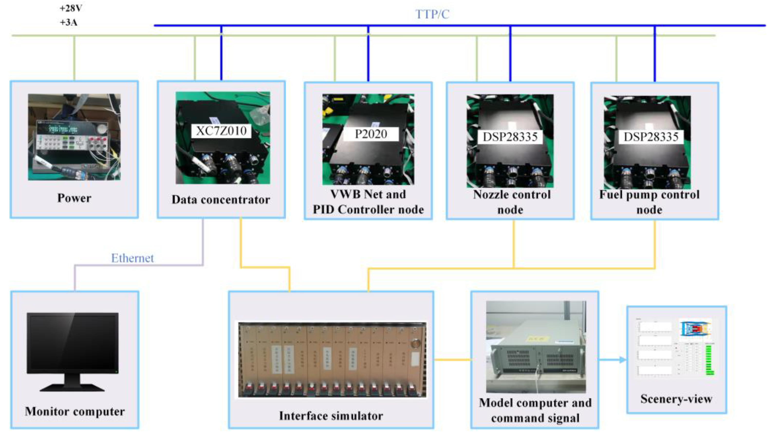
3.3. Framework of Hardware in Loop Simulation Experiment

The hardware in loop simulation has higher simulation credibility which uses the real controller in the control system simulation, therefore, we can prove the feasibility of the proposed analytical redundancy method running on the real-time embedded controller and further verify the estimation accuracy and real-time performance of the VWB Net. Figure 13 demonstrates the block diagram of the hardware in the loop simulation for a distributed engine control system. The test platform is composed of an engine model computer, monitoring computer, interface simulator, data concentrator, power, and distributed control nodes. TTP/C communication bus is used to transmit data among nodes. The core controller node employs a dual-core processor module (P2020) based on NXP QorlQ P2020.

The operation process of the test platform is as follows.

Step 1. Run the engine model in the model computer and transfer the output to the interface simulator. The interface simulator simulates relevant sensor signals, such as thermal resistance temperature sensor, piezoresistive sensor, LVDT displacement sensor, magnetoelectric speed sensor, etc. These signals are transmitted to the data concentrator, converted into digital signals, and then transmitted to the core control node through the TTP/C bus.

Step 2. There are VWB Net and PID controllers on the core control node. The core control node receives parameters of the current state and commands from the upper computer, such as speed and engine pressure ratio. VWB Net estimates the speed and engine pressure ratio. When the speed and pressure sensors fail, the estimated value replaces the sensor signal. The target fuel consumption and nozzle area are calculated by the PID controller and transmitted to each actuator control node through the TTP/C bus.

Step 3. The nozzle and fuel pump control nodes calculate the currents of the solenoid valve driving the nozzle and fuel pump, respectively. The driving currents output from actuator control nodes are acquired by the interface simulator, converted into digital signals, and then transmitted to the actuator models in the model computer.

Step 4. The actuator models calculate the updated control variables. Finally, the engine status is updated in real time.

3.4. Hardware in the Loop Simulation Experiment

When there is a bias or drift fault in pressure and speed sensors, and the estimation error of the neural network exceeds a certain threshold compared to the actual sensor value, the estimated value from the neural network is used to replace the actual sensor value. As this paper focuses on the construction of analytical redundancy and the research on its accuracy and real-time performance, the fault diagnosis method will be investigated in future studies.

In hardware in the loop simulation experiment, low-pressure rotor speed ($N_l$) and engine pressure ratio ($EPR$) dual variable control is adopted. During $N_l$ closed-loop control circuit, the controlled signal is switched between the physical $N_l$ and the analytical redundancy $N_l$ estimated by the VWB Net. During $EPR$ closed-loop control circuit, the controlled signal is switched between the physical engine pressure ratio $EPR$ and the analytical redundancy engine pressure ratio $EPR$ estimated by VWB Net.

The estimation accuracy of the analytical redundancy and the disturbance size of the actual value are important indicators to measure the reconstruction accuracy of analytical redundancy based on the VWB Net.

The steady-state estimation accuracy of the analytical redundancy is defined as

$$E{A}_R=\frac{\left|A{V}_R-E{V}_R\right|}{tar},$$

(37)

where $A{V}_R$ is the actual value when the closed-loop control circuit is using the analytical redundancy, $E{V}_R$ is the estimated value when the closed-loop control circuit is using the analytical redundancy, and $tar$ is the target value maintained.

In the following equations, $A{V}_b$ is the actual value before switching, and $A{V}_a$ is the actual value after switching.

The disturbance size of the actual value when the sensor signal is switched to the analytical redundancy signal is defined as

$$D{S}_{SR}=\frac{\left|A{V}_b-A{V}_a\right|}{tar}.$$

(38)

The disturbance size of the actual value when the analytical redundancy signal is switched to the sensor signal is defined as

$$D{S}_{RS}=\frac{\left|A{V}_b-A{V}_a\right|}{tar}.$$

(39)

Table 5. Estimation accuracy and disturbance size under $H$ = 0 km, $Ma$ = 0, and $H$ = 11 km, $Ma$ = 1.2.

Environment		${\mathit{N}}_{\mathit{l}}$	$\mathit{E}\mathit{P}\mathit{R}$
H = 0 km Ma = 0	$D{S}_{SR}$ (%)	0.09	0.34
	$D{S}_{RS}$ (%)	0.09	0.34
	$E{A}_R$ (%)	0.11	0.34
H = 11 km Ma = 1.2	$D{S}_{SR}$ (%)	0.10	0.15
	$D{S}_{RS}$ (%)	0.10	0.15
	$E{A}_R$ (%)	0.09	0.15

shows the steady-state estimation accuracy of the analytical redundancy and the disturbance size of the actual value under two distinct flight conditions. The first condition is sea level with zero Mach number ($H$ = 0 km, $Ma$= 0), while the second condition is an altitude of 11,000 meters with a Mach number of 1.2 ($H$= 11 km, $Ma$ = 1.2). Moreover, the engine mode used in this section is the dual bypass mode. We switch the controlled signal in the 45th s. The estimation accuracy and the disturbance size are less than 0.34%, meeting the requirements of VCE parameter estimation accuracy. The calculation time of the VWB Net each time in P2020 is 1.2 ms, meeting the requirements of real-time calculation. As shown in Figure 14, Figure 15, Figure 16 and Figure 17, when the controlled signal is switched between the sensor signal and the analytical redundancy signal, the engine can operate stably as before, meeting the requirements of engine-safe operation.

4. Conclusions

The analytical redundancy for the variable cycle engine (VCE) is a multi-variable, time-varying, dynamic, and highly nonlinear problem. By making weights and biases nonlinear mappings of input, variable-weights-biases neural network’s (VWB Net’s) nonlinear expressive capability is enhanced while its layers and parameters are decreased. Additionally, variable-biases can be applied at the terminal node to quickly eliminate the error between the actual sensor output and estimated value. The experiments and results under the large envelope show that VWB Net is suitable for constructing the VCE analytical redundancy. In the digital simulation experiment, based on VWB Net, the average relative errors of speed, temperature, and pressure in steady and dynamic processes are less than 0.27%. VWB Net demonstrates the best accuracy in speed analytical redundancy with only 0.19%. The calculation efficiency and parameter efficiency of VWB Net are more than 166 times higher than those of Dense net. In the hardware in the loop simulation experiment, the analytical redundancy based on VWB Net ensures the safe and stable operation of the engine. The estimation accuracy of the analytical redundancy and the disturbance size of the actual value is less than 0.34%; besides, the calculation time of VWB Net is 1.2 ms in P2020 each time which further verifies the estimation accuracy and real-time performance of VWB Net.

References

1. Wang, Y.J.; Huang, J.Q.; Pan, M.X.; Zhou, W.X. Variable-Geometry Rotating Components Modeling Based on Reference Characteristic Curves for the Variable Cycle Engine. Aerospace 2023, 10, 196. [Google Scholar] [CrossRef]
2. Wang, Y.J.; Huang, J.Q.; Pan, M.X.; Zhou, W.X. Game-Theory-Based Mode Switch Control Schedule Design for Variable Cycle Engine. Aerospace 2023, 10, 112. [Google Scholar] [CrossRef]
3. Lv, C.K.; Chang, J.T.; Bao, W.; Yu, D.R. Recent research progress on airbreathing aero-engine control algorithm. Propuls. Power Res. 2022, 11, 1–57. [Google Scholar] [CrossRef]
4. Li, L.; Shi, W. A fault tolerant model for multi-sensor measurement. Chin. J. Aeronaut. 2015, 28, 874–882. [Google Scholar] [CrossRef]
5. Cristaldi, L.; Ferrero, A.; Macchi, M.; Mehrafshan, A.; Arpaia, P. Virtual sensors: A tool to improve reliability. In Proceedings of the 2020 IEEE International Workshop on Metrology for Industry 4.0 & IoT, Rome, Italy, 3–5 June 2020; pp. 142–145. [Google Scholar]
6. Gao, Z.; Cecati, C.; Ding, S.X. A survey of fault diagnosis and fault-tolerant techniques—Part I: Fault diagnosis with model-based and signal-based approaches. IEEE Trans. Ind. Electron. 2015, 62, 3757–3767. [Google Scholar] [CrossRef]
7. Liu, S.C.; Lyu, P.; Lai, J.Z.; Yuan, C.; Wang, B.Q. A fault-tolerant attitude estimation method for quadrotors based on analytical redundancy. Aerosp. Sci. Technol. 2019, 93, 105290. [Google Scholar] [CrossRef]
8. Boomadevi, P.; Paulson, V.; Samlal, S.; Varatharajan, M.; Sekar, M.; Alsehli, M.; Elfasakhany, A.; Tola, S. Impact of microalgae biofuel on microgas turbine aviation engine: A combustion and emission study. Fuel 2021, 302, 121155. [Google Scholar] [CrossRef]
9. Zhang, L.; Lin, J.; Liu, B.; Zhang, Z.; Yan, X.; Wei, M. A review on deep learning applications in prognostics and health management. IEEE Access 2019, 7, 162415–162438. [Google Scholar] [CrossRef]
10. Pang, S.W.; Li, Q.H.; Feng, H.L. A hybrid onboard adaptive model for aero-engine parameter prediction. Aerosp. Sci. Technol. 2020, 105, 105951. [Google Scholar] [CrossRef]
11. Csank, J.; Connolly, J.W. Enhanced engine performance during emergency operation using a model-based engine control architecture. In Proceedings of the 51st AIAA/SAE/ASEE Joint Propulsion Conference, Orlando, FL, USA, 27–29 July 2015; p. 3991. [Google Scholar]
12. Zhao, Y.P.; Li, Z.Q.; Hu, Q.K. A size-transferring radial basis function network for aero-engine thrust estimation. Eng. Appl. Artif. Intell. 2020, 87, 103253. [Google Scholar] [CrossRef]
13. Volponi, A.J. Gas Turbine Engine Health Management Past, Present and Future Trends. In Proceedings of the ASME Turbo Expo: Turbine Technical Conference and Exposition, San Antonio, TX, USA, 3–7 June 2013. [Google Scholar]
14. Simon, D.; Simon, D.L. Constrained Kalman filtering via density function truncation for turbofan engine health estimation. Int. J. Syst. Sci. 2010, 41, 159–171. [Google Scholar] [CrossRef]
15. Liu, Y.; Frederick, D.K.; DeCastro, J.A.; Litt, J.S.; Chan, W.W. User’s Guide for the Commercial Modular Aero-Propulsion System Simulation (c-Mapss): Version 2. 2012. Available online: https://ntrs.nasa.gov/citations/20120003211 (accessed on 11 April 2023).
16. Lu, F.; Ju, H.F.; Huang, J.Q. An improved extended Kalman filter with inequality constraints for gas turbine engine health monitoring. Aerosp. Sci. Technol. 2016, 58, 36–47. [Google Scholar] [CrossRef]
17. Li, B.; Zhao, Y.P.; Chen, Y.B. Learning transfer feature representations for gas path fault diagnosis across gas turbine fleet. Eng. Appl. Artif. Intell. 2022, 111, 104733. [Google Scholar] [CrossRef]
18. Yongping, Z.; Jianguo, S. Fast online approximation for hard support vector regression and its application to analytical redundancy for aeroengines. Chin. J. Aeronaut. 2010, 23, 145–152. [Google Scholar] [CrossRef]
19. Li, Y.; Xu, M.; Wei, Y.; Huang, W. A new rolling bearing fault diagnosis method based on multiscale permutation entropy and improved support vector machine based binary tree. Measurement 2016, 77, 80–94. [Google Scholar] [CrossRef]
20. Rodil, S.S.; Fuente, M.J. Fault tolerance in the framework of support vector machines based model predictive control. Eng. Appl. Artif. Intell. 2010, 23, 1127–1139. [Google Scholar] [CrossRef]
21. Zhou, J.; Liu, Y.; Zhang, T. Analytical redundancy design for aeroengine sensor fault diagnostics based on SROS-ELM. Math. Probl. Eng. 2016, 2016, 8153282. [Google Scholar] [CrossRef]
22. Li, Y.; Li, D.; Sun, X.; Yi, X. Safety Boundary Extraction Using FCM and Prediction Using ELM for Aero-engine Performance Parameters. In Proceedings of the 2019 International Conference on Sensing, Diagnostics, Prognostics, and Control (SDPC), Beijing, China, 15–17 August 2019; pp. 18–23. [Google Scholar]
23. Zhang, K.; Lin, B.; Chen, J.; Wu, X.; Lu, C.; Zheng, D.; Tian, L. Aero-Engine Surge Fault Diagnosis Using Deep Neural Network. Comput. Syst. Sci. Eng. 2022, 42, 351–360. [Google Scholar] [CrossRef]
24. Du, X.; Chen, J.J.; Zhang, H.B.; Wang, J.Q. Fault Detection of Aero-Engine Sensor Based on Inception-CNN. Aerospace 2022, 9, 236. [Google Scholar] [CrossRef]
25. Liu, Y.; Meenakshi, V.; Karthikeyan, L.; Maroušek, J.; Krishnamoorthy, N.R.; Sekar, M.; Nasif, O.; Alharbi, S.A.; Wu, Y.; Xia, C. Machine learning based predictive modelling of micro gas turbine engine fuelled with microalgae blends on using LSTM networks: An experimental approach. Fuel 2022, 322, 124183. [Google Scholar] [CrossRef]
26. He, K.; Zhang, X.; Ren, S.; Sun, J. Deep residual learning for image recognition. In Proceedings of the IEEE Conference on Computer Vision and Pattern Recognition, Las Vegas, NV, USA, 27–30 June 2016; pp. 770–778. [Google Scholar]
27. Szegedy, C.; Liu, W.; Jia, Y.; Sermanet, P.; Reed, S.; Anguelov, D.; Erhan, D.; Vanhoucke, V.; Rabinovich, A. Going Deeper with Convolutions. In Proceedings of the IEEE Conference on Computer Vision and Pattern Recognition (CVPR), Boston, MA, USA, 7–12 June 2015; pp. 1–9. [Google Scholar]
28. Huang, G.; Liu, Z.; Van Der Maaten, L.; Weinberger, K.Q. Densely connected convolutional networks. In Proceedings of the IEEE Conference on Computer Vision and Pattern Recognition, Honolulu, HI, USA, 21–26 July 2017; pp. 4700–4708. [Google Scholar]
29. Qiu, X.J.; Chang, X.D.; Chen, J.; Fan, B.Q. Research on the Analytical Redundancy Method for the Control System of Variable Cycle Engine. Sustainability 2022, 14, 5905. [Google Scholar] [CrossRef]
30. Zhang, Z.H.; Huang, X.H.; Zhang, T.H. Analytical Redundancy of Variable Cycle Engine Based on Proper Net considering Multiple Input Variables and the Whole Engine’s Degradation. Int. J. Aerosp. Eng. 2021, 2021, 9959264. [Google Scholar] [CrossRef]
31. Aygun, H.; Turan, O. Exergetic sustainability off-design analysis of variable-cycle aero-engine in various bypass modes. Energy 2020, 195, 117008. [Google Scholar] [CrossRef]
Figure 1. Structure of VWB Net.
Aerospace 10 00419 g001
Figure 2. Graphic forward propagation of x 4 .
Aerospace 10 00419 g002
Figure 3. Graphic back propagation of l y 4 .
Aerospace 10 00419 g003
Figure 4. Structure of variable cycle engine.
Aerospace 10 00419 g004
Figure 5. Flowchart for data acquisition.
Aerospace 10 00419 g005
Figure 6. Segmentation of original data map.
Aerospace 10 00419 g006
Figure 7. N l analytical redundancies based on VWB Net, BPNN, and Dense net.
Aerospace 10 00419 g007
Figure 8. P 3 analytical redundancies based on VWB Net, BPNN, and Dense net.
Aerospace 10 00419 g008
Figure 9. T 5 analytical redundancies based on VWB Net, BPNN, and Dense net.
Aerospace 10 00419 g009aAerospace 10 00419 g009b
Figure 10. N l analytical redundancies based on VWB Net, BPNN, and Dense net.
Aerospace 10 00419 g010
Figure 11. P 3 analytical redundancies based on VWB Net, BPNN, and Dense net.
Aerospace 10 00419 g011aAerospace 10 00419 g011b
Figure 12. T 5 analytical redundancies based on VWB Net, BPNN, and Dense net.
Aerospace 10 00419 g012aAerospace 10 00419 g012b
Figure 13. Hardware in the loop experiment overall setup.
Aerospace 10 00419 g013
Figure 14. H = 0 km M a = 0, Maintain N l 9500 r/min through low-pressure rotor speed closed-loop control.
Aerospace 10 00419 g014
Figure 15. H = 0 km M a = 0. Maintain E P R 3.5 through engine pressure ratio closed-loop control.
Aerospace 10 00419 g015
Figure 16. H = 11 km M a = 1.2. Maintain N l 11,500 r/min through low-pressure rotor speed closed-loop control.
Aerospace 10 00419 g016
Figure 17. H = 11 km M a = 1.2. Maintain E P R 4.0 through engine pressure ratio closed-loop control.
Aerospace 10 00419 g017