Abstract
Supersonic shock wave boundary layer interactions are common to inlet flows of supersonic and hypersonic vehicles. This paper reports on wall-resolved implicit large-eddy simulations of a canonical Mach 2.5 turbulent shock wave boundary layer interaction experiment at the NASA Glenn Research Center. The boundary layer upstream of the interaction was nominally axisymmetric and two-dimensional. A conical centerbody with a 16 deg half-angle and a maximum radius of of the test section diameter was employed to generate a conical shock wave, where D is the test section diameter. Asymmetric (swept) interactions were obtained by displacing the shock generator away from the test section centerline. The present simulation is for a shock generator displacement of . Results from the asymmetric simulation are compared with results from an earlier simulation of a corresponding axisymmetric interaction. The experimental Reynolds number based on test section diameter was . For the simulations, the Reynolds number was lowered to to keep the computational expense of the simulations within limits. Compared to the axisymmetric interaction, the streamwise extent of the separation varies considerably in the azimuthal direction for the asymmetric interaction. The separation is strongest at the azimuthal location that is closest to the shock generator. The streamwise extent of the separated flow regions is noticeably reduced and substantial crossflow is observed between the locations that are closest and farthest from the shock generator. A Fourier analysis of the unsteady flow data indicates low-frequency content for the separated region that is closest to the shock generator. Away from this region, with increasing sweep angle and cross-flow, the low-frequency content is diminished. A proper orthogonal decomposition captures spanwise coherent structures for the more two-dimensional parts of the interaction.
1. Introduction
Shock wave boundary layer interactions (SBLI) are common to high speed engine inlet flows. Typically, SBLI lead to thicker boundary layers or flow separation, which increases total pressure losses and flow distortion, with an overall negative impact on aerodynamic performance. Shock wave-induced separation of turbulent boundary layers can be subject to large-scale, low-frequency unsteadiness [1,2,3]. The low-frequency unsteadiness is undesirable for both structure and combustion. Despite various proposed explanations for the low-frequency unsteadiness, its origin is still a matter of debate. Agostini et al. [4] conducted research on the correlation between a low-frequency bubble breathing at a Strouhal number based on boundary layer thickness of and mid-frequency convective structures with .
Most SBLI research has focused on nominally two-dimensional (2D) interactions, for example SBLI induced by impinging oblique shock waves [2,5,6,7] and compression ramps [6,8,9]. The motivation behind prioritizing the investigation of 2D interactions before delving into more complex three-dimensional (3D) SBLI is rooted in the need to comprehend the underlying flow physics at a fundamental level. Unfortunately, few studies address the question of when and how the fundamental flow physics of 2D SBLI carry over to 3D SBLI. This serves as the impetus for conducting 3D SBLI research. A recent overview highlighting some of the key differences between 2D and 3D SBLI and notable findings in 3D SBLI research was provided by Gaitonde and Adler [10]. One key difference between 2D and 3D interactions is that, for the latter, the streamlines inside the recirculation region do not form closed loops, but instead spiral outward in the spanwise direction [11]. Additionally, compared to 2D interactions, the mid-frequency component for 3D interactions has been found to be more prominent downstream of the separation line [12]. A differentiation is made between 3D interactions with conical and cylindrical symmetry [13]. While a global separation length can easily be defined for 2D SBLI, this is not possible for 3D SBLI with conical symmetry [14]. Therefore, the Strouhal number for 3D SBLI is often based on the incoming boundary layer thickness. To generate a swept interaction, Huang et al. [15] positioned a slanted step with a height that varied azimuthally over an axisymmetric turbulent boundary layer. They observed an increase in the shock “pulsation” frequency in the swept separation region for sweep angles less than where a downstream feedback mechanism is enabled by recirculation. Arora et al. [16] conducted unsteady surface pressure measurements for a Mach 2 swept SBLI that was set up with a fin. Compared to unswept 2D SBLI, which typically exhibit a dominant low-frequency content with , they observed that the mid-frequency fluctuations in the swept SBLI were more pronounced, falling within the range of . By contrasting a swept interaction with a corresponding 2D interaction, Adler and Gaitonde [17] pinpointed a convective instability unique to the 3D interaction that amplifies the incoming boundary layer disturbances. In contrast, the 2D SBLI displayed an absolute instability. Lee and Gross [18] investigated unswept and swept interactions with cylindrical symmetry and found that the low-frequency unsteadiness was suppressed with increasing sweep angle.
Of the scarce amount of 3D SBLI research, the majority has primarily focused on sharp fins [19,20,21], swept compression ramps [22,23], and swept impinging oblique shock waves [6,24,25]. Some recent work by Zuo et al. [26] considered the interaction of a conical shock wave with a flat plate boundary layer. The interaction of a conical shock wave with an axisymmetric boundary layer to produce a purely 2D SBLI has been addressed in only a handful of publications [27,28]. Such interactions are not only highly relevant for circular inlet flows but also help avoid issues faced in SBLI experiments in rectangular test sections [29,30], such as corner effects, which are exacerbated in the presence of crossflow and 3D flow features. To date, only two asymmetric constant-strength shock interactions (i.e., shock-generator cone displaced from centerline) in axisymmetric test sections have been performed [31,32] and no accompanying high-fidelity simulations exist. Unfortunately, the experiment by Chou [31] was not included in the computational fluid dynamics (CFD) validation assessment by Settles and Dodson [33]. We present the first simulation of an asymmetric SBLI in a nominally asymmetric experiment.
Recent Mach 2.5 axisymmetric SBLI experiments conducted at the NASA Glenn Research Center by Davis, Sasson, Reising and others [28,32,34,35,36] were nominally symmetric in the azimuthal direction, which eliminated geometric complexity and also solved the finite span effect problems encountered in flat-plate SBLI experiments. In addition, the experiment’s nominal symmetry in the azimuthal direction renders it more suitable for simulations. Lastly, the experiments can be considered canonical, as they represent actual inlet flows but with reduced geometric complexity, which facilitates the extraction and comprehension of the fundamental flow physics. The experiment utilized shock generators with a half-angle of and cylindrical support to produce conical shock waves, along with expansion fans, which impacted a turbulent boundary layer on the interior surface of a cylindrical test section with a diameter of 17 cm. The radii of the cylindrical centerbodies were 1.57 cm and 2.5 cm. Swept interactions were produced by displacing the shock generator from the centerline of the test section. In the experiments with a shock generator radius of cm, the shock generator was displaced from the centerline by cm and cm.
This paper reports on wall-resolved implicit large eddy simulation (ILES) of the asymmetric interaction for the larger centerbody radius (2.5 cm) and offset position of one-third of the test section radius (). Initial and boundary conditions for the implicit large eddy simulation (ILES) were obtained from Reynolds-averaged Navier–Stokes (RANS) calculations. For the simulations, the Reynolds number was reduced from (the experimental Reynolds number [28]) to to relax the grid resolution requirements. In the following, first, the experiment is briefly described in Section 2. Section 3 then discusses the numerical methods and setup of the simulations are introduced. Section 4 will examine the instantaneous and time-averaged data acquired from the ILES, with a particular emphasis on analyzing the separation topology and the intensity of the unsteady flow content. Here, detailed comparisons are made with earlier ILES results of a corresponding axisymmetric interaction [37]. Section 5 provides a concise summary and thorough analysis of the results, concluding the paper.
2. Experiment
The present simulations are modeled after the Mach 2.5 turbulent SBLI experiments by Davis [28] in the axisymmetric supersonic circular wind tunnel (Axi-SWT) at the NASA Glenn Research Center (GRC). The experiments were designed to provide validation data for CFD analyses and turbulence model development. The circular test section had an inner diameter of cm ( cm). Air with a freestream temperature and pressure of 132 K and 22,065 Pa was used as the working medium. The Reynolds number, which was based on the diameter of the test section and the approach flow velocity, was . A cylindrical centerbody with 1.57 cm or 2.5 cm radius with a conical tip was employed for generating a conical shock wave and expansion fan. For the nominally axisymmetric (here also referred to as nominally 2D) experiments, the shock generator was placed on the centerline and the boundary layer momentum thickness Reynolds number prior to separation was . The flow physics were more interesting for the larger centerbody which produced a stronger interaction. The conical shock wave was reflected at the cylindrical test section wall and then at the centerbody, leading to a secondary, weaker SBLI on the test section wall. Three different shock generator cone half-angles were employed in the experiments, , , and . In order to keep the inviscid shock impingement location the same, the shock generator was shifted downstream for the larger cone half-angles. For the half-angle, Davis [28] did not observe any flow separation from the wind tunnel wall. For the and half-angles, the interaction was stronger and the flow separated from the tunnel wall. Swept (asymmetric) interactions were obtained by a parallel offset of the shock generator from the centerline [28,32,34,35,36]. Two shock generator offsets from the centerline, cm and cm, were considered. Wall pressure measurements (mean only) were taken to characterize the resulting asymmetric interactions. In addition, profiles of the streamwise velocity, total pressure, and root-mean-square velocity fluctuations were obtained.
3. Computational Methods
3.1. Overview of Simulations
A wall-resolved implicit large-eddy simulation (ILES) of the Mach 2.5 experiment with shock generator radius and cone half angle of 2.5 cm (made dimensionless with the test section diameter, ) and , respectively, and shock generator offset from the centerline of cm (asymmetric case) was carried out. Out of the cases considered in the experiments [28,32,35], this case has the largest crossflow component and is most interesting with respect to the unsteady flow physics. The results obtained from the present simulation are compared with those from an earlier simulation by Mosele et al. [37] for a corresponding axisymmetric case (shock generator aligned with the test section centerline, same shock generator radius and cone half angle). The same simulation strategy that was employed earlier by Mosele et al. [37] for the axisymmetric simulation, was also employed for the present asymmetric simulation. The initial step involved conducting a precursor Reynolds-averaged Navier–Stokes (RANS) calculation to acquire data for the initialization of the ILES and for the inflow and freestream boundary conditions. Following Mosele et al. [37], the Reynolds number (based on test section diameter) was lowered from (experiments) to for the ILES to save computational resources. Souverein et al. [38] demonstrated that for turbulent boundary layers, the onset of flow separation is nearly independent of the Reynolds number. The interaction length was found to scale with the displacement thickness of the upstream turbulent boundary layer. Furthermore, Baldwin et al. [21] showed that compared to the shock generator angle and freestream Mach number, which determine the interaction strength, the Reynolds number is a secondary factor in governing the interaction. Additionally, the sensitivity of the flow to the Reynolds number was found to decrease for higher Reynolds numbers and stronger interactions.
3.2. Governing Equations and Discretization
A compressible finite-volume Navier–Stokes code [39,40] was employed for the axisymmetric and asymmetric precursor RANS calculations and the ILES. The viscosity was obtained from Sutherland’s law and the heat conduction coefficient was obtained from , where is the dynamic viscosity, is the specific heat at constant pressure, and is the Prandtl number. Ninth-order and fourth-order accurate discretizations were employed for the convective and viscous terms of the Navier–Stokes equations. For the RANS equations, a discretization with second-order accuracy was utilized.
For the RANS calculations, both the Favre-averaged compressible Navier–Stokes equations and the k- turbulence model equations,
were solved. Here, k is the turbulence kinetic energy, is the specific dissipation rate, and
is the eddy viscosity. Wilcox [41] provides information on the compressibility corrections, as well as the model constants. Due to its demonstrated ability to accurately predict shock-separated flows, the k- model [42] was selected for the precursor RANS calculations. For calculating the Reynolds stresses, the Boussinesq approximation was utilized. The highly dissipative first-order-accurate Euler backward scheme was used for time integration because steady state RANS solutions were being sought.
For the ILES, the compressible Navier–Stokes equations were directly solved without turbulence modeling. This approach is justified when the numerical diffusion of the discretization drains the proper amount of energy at the smallest resolved scales, similar to subgrid stress models in explicit large-eddy simulations (LES). The Navier–Stokes equations were integrated in time with the second-order-accurate trapezoidal rule.
3.3. Non-Dimensionalization
Velocities and density were made dimensionless with the upstream freestream values, and , respectively. The asterisks indicate dimensional quantities. All length scales were made dimensionless by the inner diameter of the test section, cm, and time was normalized by . The test section radius was cm or . The laminar and eddy-viscosity were made dimensionless by the freestream dynamic viscosity, . The turbulence kinetic energy was made dimensionless by and the dissipation rate was made dimensionless by . The laminar and turbulent Prandtl numbers were and and the freestream Mach number was 2.5. The reference Reynolds number for the simulations was and, thus, 10 times smaller than in the experiments [28,32,35]. The dimensionless computational time-step for the precursor RANS calculation was . The time-step for the ILES was . This time-step corresponds to (in dimensional form), (in wall units based on approach boundary layer), and (based on boundary layer thickness, ).
3.4. Computational Grids
If the shock generator is not aligned with the centerline, the flow field becomes 3D and symmetry conditions can only be applied in relation to the plane that intersects the test section and the shock generator centerline at (the current setup’s reference plane). As a result, the computational domain for the RANS calculation and ILES had to span half of the circumference (180 degrees). Using analytical functions, a 3D grid for the precursor RANS calculation with centerbody offset of was generated. The inflow and outflow boundaries were positioned at and , respectively. The location corresponds to the start of the test section in the experiment. The number of cells in the axial, radial, and azimuthal direction was . Because the freestream was quiescent, the grid resolution requirement outside the boundary layer is low and grid line stretching was employed away from the walls. An outline of the 3D computational domain for the asymmetric RANS calculation is provided in Figure 1. Figure 2 presents a cross-sectional view of the RANS grid at the outflow.
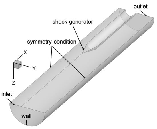
Figure 1.
Outline of computational domain for asymmetric RANS calculation.
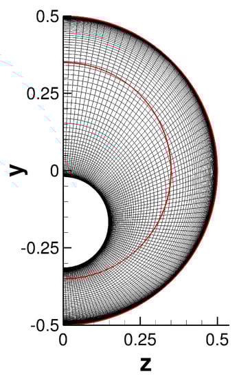
Figure 2.
Cross−sectional view of computational grid (outflow boundary) for asymmetric RANS calculation. The axes are made dimensionless by the test section diameter, D. The computational domain boundaries for the ILES are delineated in red.
The computational grid for the asymmetric ILES was generated from a 2D grid (Figure 3),
where is the azimuth angle. The computational grid is axisymmetric (Figure 4) and the asymmetry of the flow is introduced through the freestream boundary conditions. The grid has the same near-wall grid resolution (axial, radial, and azimuthal) as the grid for the earlier ILES of the corresponding axisymmetric interaction with equal shock strength (, deg) [37]. While the grid opening angle for the earlier ILES of the axisymmetric interaction was , the grid for the asymmetric ILES spans over an azimuth angle of (Figure 4). To prevent the grid from intersecting with the shock generator, the radial extent of the grid was reduced from (as in previous axisymmetric simulations) to (as shown in Figure 2, where the ILES grid boundaries are highlighted).
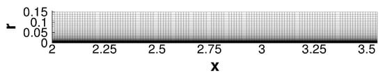
Figure 3.
Computational grid for ILES of asymmetric interaction. To enhance clarity, every other grid line in the wall-normal direction was excluded, while every seventh grid line was included in the streamwise direction.
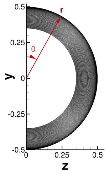
Figure 4.
Cross—sectional view of computational grid for asymmetric ILES. To improve clarity, every other grid line was excluded in both the wall−normal and spanwise directions. The r and directions of the cylindrical coordinate system are included for future reference (marked in red).
The grid resolution for the ILES of the asymmetric interaction was based on an earlier grid resolution study for the axisymmetric cases [37]. The approach boundary layer near-wall grid resolution in wall units, , in the axial, radial, and azimuthal (at ) direction, the domain extent, and the number of cells, , of the computational grids for the earlier axisymmetric ILES and present asymmetric ILES are summarized in Table 1. Additionally included in the table is the total number of cells, . Because the 3D grid covers a larger azimuth, the total number of cells, , is considerably larger than for the earlier axisymmetric simulation. Further details on the computational grid can be found in Ref. [37].

Table 1.
Computational grid parameters. Inner-scale variables calculated at .
A grid-resolution study was previously performed for the axisymmetric SBLI with and deg. Since the same shock generator (both radius and cone half-angle) was used for the present asymmetric interaction, the efficacy of the grid resolution did not need to be reassessed. The previous grid resolution study for the axisymmetric interaction [37] is briefly summarized next. In addition to the baseline grid (present grid resolution), three additional computational grids with approximately 1.5 times improved grid resolution in all three dimensions were generated to investigate grid convergence of the solution. The number of cells and near-wall resolution (upstream of the interaction) for the different cases are compared in Table 2. Van Driest-transformed velocity profiles and skin-friction distributions revealed that for all three refined meshes, no significant change in the solution was observed compared to the baseline grid. Therefore, to significantly reduce the computational cost, all computational grids for the present work have the same near-wall grid resolution as for the earlier baseline grid.
Table 2.
Computational grid parameters for earlier grid resolution study [37]. Inner-scale variables calculated at .
Unlike for the previous axisymmetric ILES [37], where the turbulence statistics were obtained in two steps, for the asymmetric ILES the time average and turbulence statistics were computed simultaneously over a time interval of 48 non-dimensional time units.
3.5. Boundary Conditions
Dirichlet boundary conditions were enforced at the inflow and Neumann boundary conditions were invoked at the outflow boundary. The inflow freestream conditions were matched to those of the experiment at the NASA GRC facility [28,32]. For the RANS calculations, a laminar inflow was assumed and the inflow turbulence intensity and eddy viscosity ratio were set to and . All walls were considered to be adiabatic. For the earlier axisymmetric ILES with 20 degrees azimuthal domain extent [37], flow periodicity was enforced in the circumferential direction. For the present ILES of the asymmetric interaction (with 180 degree azimuthal domain extent), symmetry boundary conditions were enforced at the lateral domain boundaries.
For the ILES, the RANS solution was prescribed at the inflow and freestream boundary. Since the RANS and ILES grid lines did not coincide, a radial basis function (RBF) approach [43] was employed for interpolating the RANS solution on the freestream boundary of the ILES domain. Firstly, the nearest cell on the RANS grid was determined for every cell situated on the freestream boundary of the ILES grid. Subsequently, an RBF interpolation was calculated across a volume that encompassed the neighboring cells (of the RANS grid) in all three dimensions. This led to a linear system of size or 125,
where s denotes the variable interpolated onto the ILES grid, represents the position vector, is the weight and is the RBF. In the other regions (excluding the freestream boundary), the nearest available RANS solution was utilized to initialize the ILES flow field.
The inflow momentum thickness Reynolds number for the ILES was . The isotropic divergence free (for incompressible flow) synthetic eddy model (SEM) by Poletto [44] was employed to “seed” turbulent velocity fluctuations inside the inflow boundary layer. The temperature fluctuations were obtained from the strong Reynolds analogy,
with . Here, the prime indicates fluctuations and the overbar indicates a mean value. Further details on the implementation of the SEM and the streamwise development of the turbulent inflow boundary layer can be found in Mosele et al. [37].
3.6. Proper Orthogonal Decomposition
The proper orthogonal decomposition (POD) [45] was employed to analyze the unsteady wall-pressure data [46]. The POD decomposes an unsteady pressure field into time coefficients and modes (or eigenfunctions),
The “snapshot” method by Sirovich [47] is well suited for the analysis of discrete time sequences from simulations and was also employed for the present analysis. The POD kernel was based on the wall-pressure coefficient, such that the magnitude of the POD eigenvalues, , is of order . The POD then provides an energy-optimal decomposition that captures the largest amount of kinetic energy with the least number of modes.
4. Results
A numerical schlieren image from the Mach 2.5 asymmetric precursor RANS calculation taken in the plane (Figure 5) outlines the general flow topology. The incident conical shock wave impinges on the turbulent boundary on the test section wall (primary SBLI). The impingement point is further upstream on the bottom where the shock generator is closest to the test section wall, and further downstream on the top where the shock generator is farthest from the test section wall. An expansion fan emanates from the downstream end of the conical shock generator. On the top, the expansion fan hits the wall at about the same streamwise location as the impinging shock wave. On the bottom, the expansion fan reaches the wall downstream of the impingement point. On both sides, the incident shock wave is reflected off the wall and impinges on the centerbody where it causes the boundary layer to separate. The reflected shock wave is then reflected off the centerbody and impacts the test section wall a second time, resulting in a secondary, weaker SBLI.
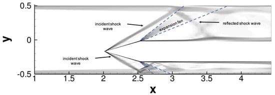
Figure 5.
Numerical schlieren image obtained from precursor asymmetric RANS calculation ( plane). The dashed lines delineate the start and end of the expansion fans.
4.1. Turbulent Approach Boundary Layer
The properties of the upstream boundary layer in the simulations were matched to the experiment (see [37] for full details). In the precursor RANS calculations, the streamwise extent of the approach boundary layer was varied until the boundary layer thickness and shape factor approximately matched the experiment at . The upstream boundary layer properties of the experiment [28,32] and the precursor RANS calculations (which provided the inflow and initial conditions for the ILES) are provided in Table 3.
Table 3.
Turbulent boundary layer properties at .
The boundary layer properties shortly upstream of the interaction at , obtained from both experiment and axisymmetric ILES, are in reasonable agreement (see Table 4). The difference between the boundary layer properties for the experiment and axisymmetric ILES is due to the fact that the RANS calculations were matched to the experiment further upstream.
Table 4.
Turbulent boundary layer properties at .
In Figure 6, the wall-pressure coefficient, , distributions obtained from the ILES and precursor RANS calculations are compared with experimental measurements (at the 10 times larger Reynolds number). For the axisymmetric interaction, across the interaction region, the wall-pressure coefficient is in good agreement with the experiment. Compared to the experiment, the flow separates slightly earlier. For the asymmetric interaction, the pressure distributions exhibit a strong dependence on the azimuth. Because of the larger boundary layer thickness for the simulations, the effective nozzle expansion ratio is smaller than in the experiment and as a result the core-flow pressure is larger. This explains the slight mismatch of the pressure coefficient upstream of the interaction.
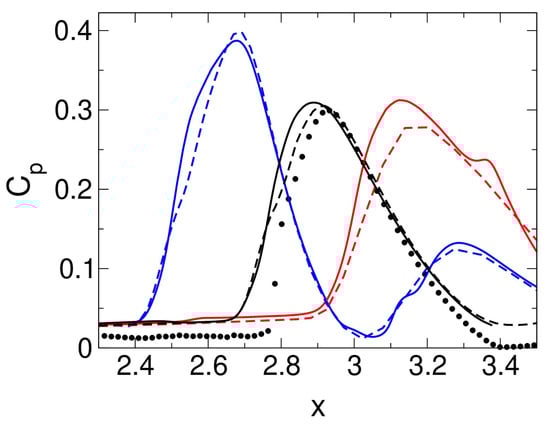
Figure 6.
Wall-pressure distributions obtained from temporal averages. Symbols are measurements by Davis et al. [28] for axisymmetric interaction at . Solid and dashed black lines are for ILES and RANS of axisymmetric interaction. Solid and dashed red () and blue () lines are for ILES and RANS of asymmetric interaction.
4.2. Instantaneous Flow Fields
Instantaneous iso-surfaces of the magnitude of the density gradient obtained from the earlier axisymmetric and current asymmetric ILES are provided in (Figure 7a). For the visualization of the axisymmetric interaction, the domain was repeated 180 deg/20 deg = 9 times in the azimuthal direction. In a similar fashion, the axisymmetric data were also repeated in the following figures, whenever appropriate. For clarity and improved orientation when interpreting the flow fields, the shock generator was added, although it was not included in the simulations. The iso-surfaces (Figure 7a) reveal the incident and reflected shock waves. For the asymmetric interaction, the interaction of the conical shock wave with the test section wall is asymmetric with respect to the test section centerline. Visualizations of the Q-criterion by Hunt [48] reveal turbulent flow structures in the approach boundary layer, as well as near and downstream of the interaction region.
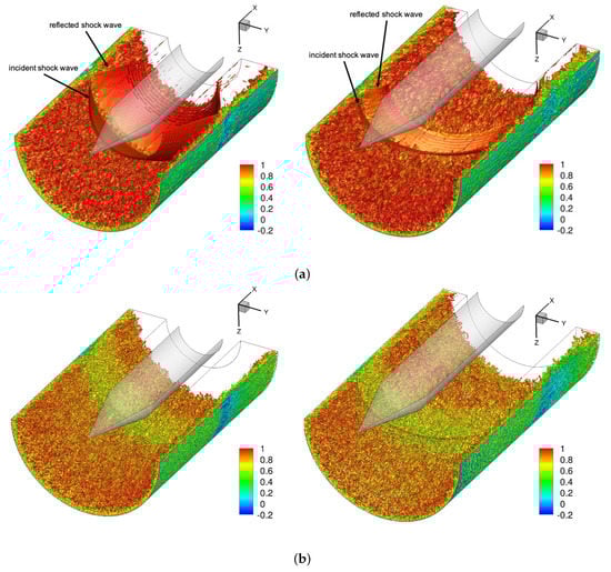
Figure 7.
Instantaneous iso-surfaces of (a) and (b) flooded by axial velocity for axisymmetric (left) and asymmetric (right) interaction.
4.3. Mean Flow Analysis
Profiles of the axial () and tangential () velocity for the axisymmetric (azimuthal average) and asymmetric interaction (for different locations) are compared in Figure 8 for different x-locations. The velocity scale is shown on the top of the profiles. The dotted lines indicate the incident and reflected shock waves. The profiles for the axisymmetric case (Figure 8a) are discussed first. The streamwise velocity profile at indicates weak reverse flow very close to the wall. The jump in the velocity profile near is due to the incident shock wave. The profile for (slightly downstream of reattachment) indicates a velocity deficit near the wall and a sudden velocity decrease at due to the reflected shock wave. The velocity deficit is also seen in the profiles for and . The azimuthal velocity component is zero for the axisymmetric interaction.
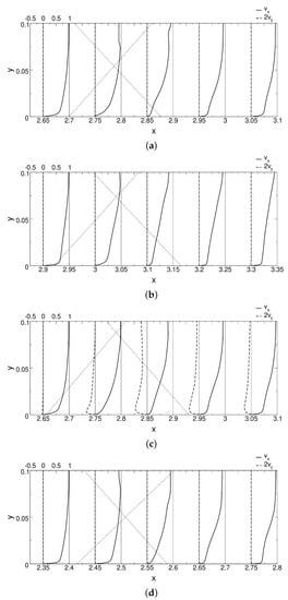
Figure 8.
Profiles of axial () and tangential () velocity for (a) axisymmetric and (b–d) asymmetric case for (b) , (c) , and (d) . The dotted lines indicate the incident and reflected shock waves.
The approach flow profiles for the axisymmetric and asymmetric interactions at are similar (Figure 8a,c). When comparing the axial velocity profiles for () and (), the near-wall velocity deficit for the latter is more pronounced, suggesting stronger flow separation. The azimuthal velocity is zero for and (symmetry plane). For , throughout the interaction the azimuthal velocity profiles are wall jet-like and feature an inflection point, which may support crossflow instability. The maximum crossflow velocity is about 25% of the freestream velocity.
The mean wall-pressure coefficient was plotted versus the axial and azimuthal coordinate (Figure 9). The black lines in Figure 9 indicate the inviscid shock impingement lines on the test section wall. The inviscid impingement lines follow the relationship,
The offset position, , is zero for the axisymmetric interaction and for the asymmetric interaction. Furthermore, is the axial location of the tip of the shock generator and is the shock angle. The shock angle was obtained from a numerical solution of the Taylor–Macoll equation [49]. For both cases, the pressure increases upstream of the inviscid impingement line. While the pressure increase is independent of the azimuth for the axisymmetric interaction, for the asymmetric interaction it varies strongly in the azimuthal direction. In agreement with Sasson et al. [32], the pressure increase is strongest on the side that is closest to the shock generator () and smallest for , where the impingement line is highly swept with respect to the freestream direction. The pressure increase is followed by an expansion and, for the asymmetric case, a secondary weaker pressure increase.
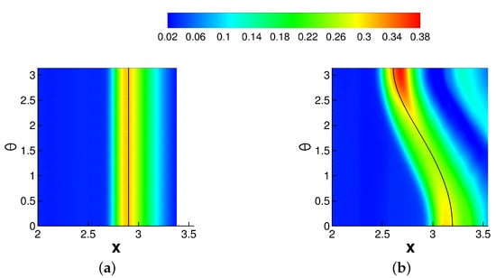
Figure 9.
Wall-pressure coefficient contours and inviscid shock impingement line (solid black line) for (a) axisymmetric and (b) asymmetric interaction.
In Figure 10, iso-contours of the mean axial velocity, , radial velocity, , and tangential velocity, , from the earlier axisymmetric ILES (azimuthal average) [37] and the present asymmetric ILES are compared. For , the distance of the shock generator from the wall matches that of the concentric configuration. Compared to the axisymmetric interaction, for the asymmetric interaction the SBLI is located slightly farther downstream (Figure 10a). The radial velocity contours (Figure 10b) suggest a larger streamwise offset between the incident and reflected shock waves for the asymmetric case. The tangential velocity component (Figure 10c) is noticeably absent for the axisymmetric interaction and negative for the asymmetric interaction, suggesting flow from the high-pressure region at to the low-pressure region at .
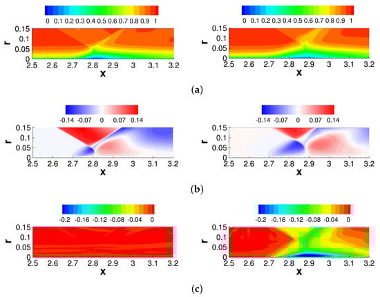
Figure 10.
Iso-contours of (a) axial, (b) radial, and (c) tangential velocity for axisymmetric interaction [37] (left) and asymmetric interaction at (right).
Contours of the magnitude of the skin-friction coefficient and skin-friction lines are shown in Figure 11. For the axisymmetric interaction, the separation and reattachment lines are straight (the end points are labeled “S” and “R” in the figure). For the asymmetric interaction, a saddle point (“S”) and node (“R”) of reattachment are located at both and . Lines of separation and reattachment that originate from the critical points converge near suggesting that the separation does not cover the entire azimuth. According to Tobak and Peake [50], since the separated flow regions close without a critical point, they can be classified as “open”. The lines of separation and reattachment are not parallel to each other but diverging away from . According to the classification by Settles [13], swept interactions with diverging separation and reattachment lines are classified as “conical”.
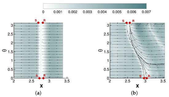
Figure 11.
Skin-friction magnitude iso-contours and skin-friction lines for (a) axisymmetric and (b) asymmetric case.
Figure 12 displays iso-contours of the axial skin-friction coefficient in addition to skin-friction lines. As indicated by the blue region in Figure 12a, for the axisymmetric case, the flow remains separated across the azimuth. For the asymmetric case (Figure 12b), in the mean, the flow is attached near . Strong reverse flow occurs near and weak reverse flow is observed near (Figure 12b).
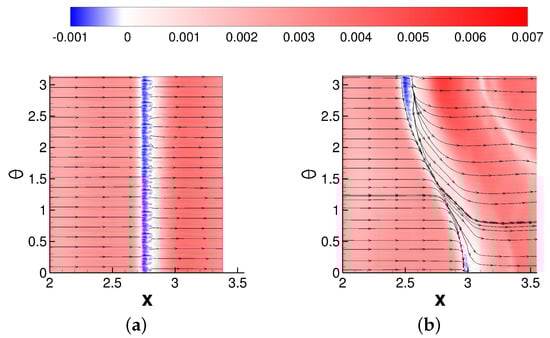
Figure 12.
Axial skin-friction coefficient iso-contours and skin-friction lines for (a) axisymmetric and (b) asymmetric case.
The average separation length was computed by identifying the point at which the axial skin-friction coefficient changes sign (Figure 13). The separation length was calculated using both raw data (blue lines) and raw data that underwent streamwise and azimuthal filtering (black lines). The separation length for the asymmetric interaction is larger for the side on which the centerbody is closer to the test section wall, . On this side, it roughly matches the separation length of the axisymmetric interaction. On the other side, , the separation is weaker and shorter than for the axisymmetric interaction. For , the flow remains attached in the mean. Across the azimuth, the streamwise extent of the separation for the asymmetric case does not exceed that of the axisymmetric case.
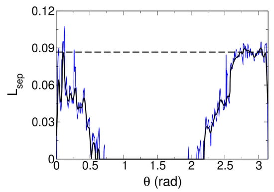
Figure 13.
Axial separation length for the asymmetric (solid lines) and axisymmetric (dashed line) case [37]. The blue line represents the unfiltered data for the asymmetric case.
Considerable crossflow for the asymmetric case is revealed by the iso-contours of the azimuthal component of the skin-friction coefficient, as shown in Figure 14. Beginning at separation and extending downstream of reattachment, there is a region of strongly negative azimuthal skin-friction (indicated by the blue region). The direction of the flow is away from the high-pressure region directly underneath the shock generator and towards the side that is furthest from the shock generator. A similar large flow turning across the interaction was observed by Chou [31] and Sasson [32]. The crossflow is strongest near , as indicated by the azimuthal skin-friction coefficient contours and the skin-friction lines (Figure 14b). The presence of the reflected shock wave can be linked to a second region located further downstream, where the skin-friction coefficient in the azimuthal direction is negative.
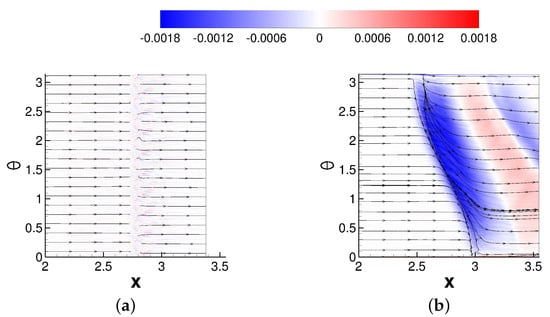
Figure 14.
Azimuthal skin-friction iso-contours and skin-friction lines for (a) axisymmetric and (b) asymmetric case.
In Figure 15, the minimum axial skin-friction coefficient (), as well as the minimum and maximum azimuthal skin-friction coefficients () are plotted as functions of the azimuth angle. For the axisymmetric interaction, all three quantities indicate symmetry in the azimuthal direction. For the asymmetric interaction, the axial skin-friction coefficient goes negative (indicating recirculation) near the domain boundaries ( and ). For the side that is closer to the shock generator (), the axial skin-friction coefficient exhibits a more negative value. This is also the only region where the magnitude of the axial skin-friction coefficient exceeds that of the axisymmetric interaction. The azimuthal skin-friction coefficient obtains a large negative value near , again indicating a substantial flow away from the high-pressure region at .
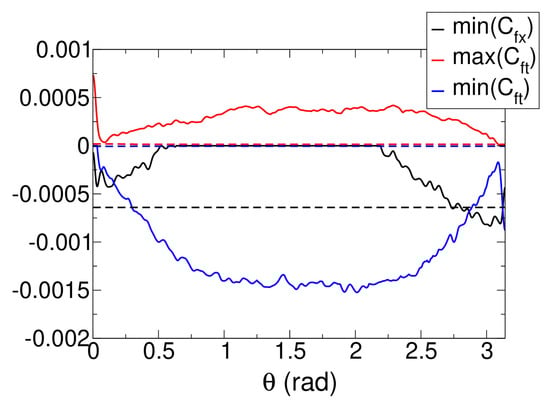
Figure 15.
Minimum and and maximum (in axial direction) for axisymmetric (dashed lines) and asymmetric (solid lines) case.
In Figure 16, the minimum (in x and r) azimuthal velocity, , is plotted against the azimuth. The asymmetric interaction exhibits a region of intense crossflow near where the azimuthal velocity is about 23% of the approach freestream velocity.
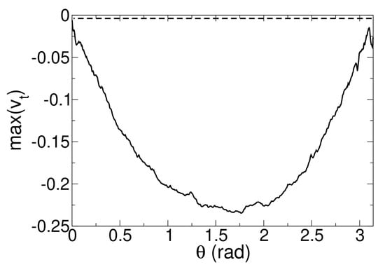
Figure 16.
Minimum for axisymmetric (dashed line) and asymmetric (solid line) case.
4.4. Turbulent Statistics
The root-mean-square (RMS) velocity fluctuations and turbulence kinetic energy (TKE) are compared in Figure 17 and Figure 18 and the Reynolds shear stresses are compared in Figure 19 and Figure 20. To allow for a more direct comparison, for the asymmetric interaction the abscissa was shifted by the inviscid shock impingement location, , corresponding to the respective azimuth, . For the asymmetric interaction, azimuths of (furthest from shock generator), (same distance to shock generator as for axisymmetric interaction), and (closest to shock generator) are shown.
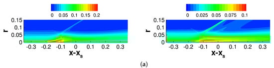
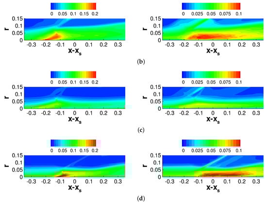
Figure 17.
Iso-contours of (left column) and (right column) for (a) axisymmetric and asymmetric case at (b) , (c) and (d) .
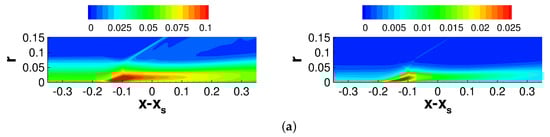
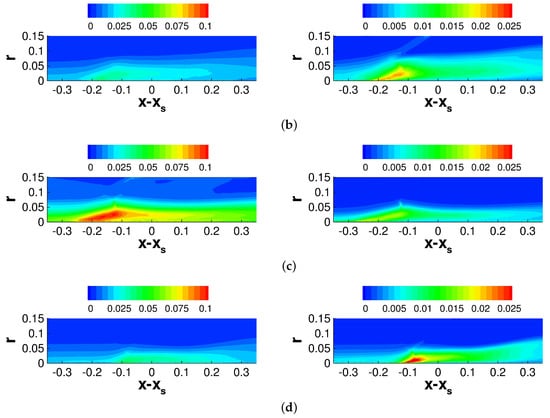
Figure 18.
Iso-contours of (left column) and k (right column) for (a) axisymmetric and asymmetric case at (b) , (c) and (d) .
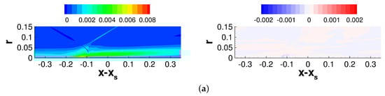
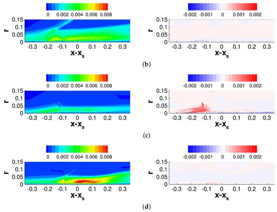
Figure 19.
Iso-contours of (left column) and (right column) for (a) axisymmetric and asymmetric case at (b) , (c) , and (d) .
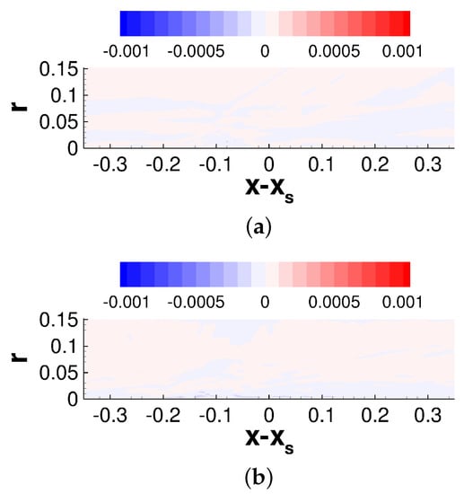
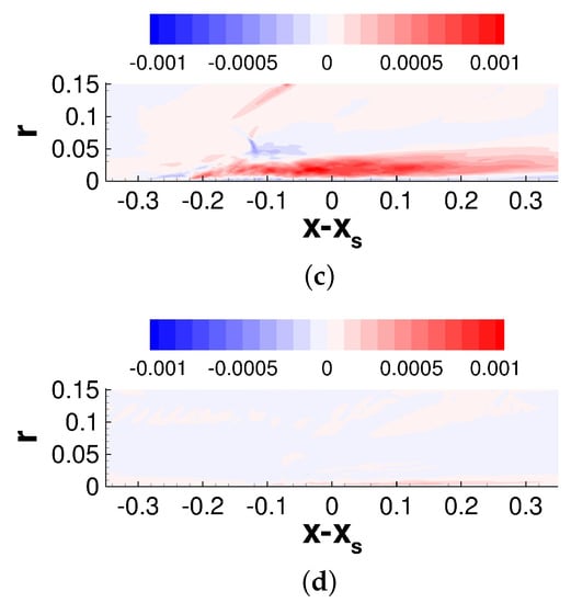
Figure 20.
Iso-contours of for (a) axisymmetric and asymmetric case at (b) , (c) , and (d) .
The RMS velocity fluctuations and TKE distributions (Figure 17 and Figure 18) are discussed first. The axial fluctuations, , are largest at separation (Figure 17, left column), possibly indicating an axial back and forth motion of the separation shock foot. For the asymmetric case, at the crossflow is strong (Figure 10c and Figure 16), separation is suppressed (Figure 13 and Figure 15) and the axial fluctuations are much smaller than for the axisymmetric case. On the other hand, for (furthest from shock generator) and even more so for (closest to shock generator) the crossflow is negligible, the flow is separated, and the axial fluctuations are stronger than for the axisymmetric interaction.
Large wall-normal velocity fluctuations, , downstream of the reflected shock foot suggest a flapping motion of the shear layer (Figure 17, right column). For the asymmetric interaction, the strong crossflow and suppressed separation for go hand in hand with lower wall-normal velocity fluctuations compared to the axisymmetric case. For and , the wall-normal fluctuations are considerably stronger than for the axisymmetric interaction and reach farther downstream of the interaction region.
The azimuthal velocity fluctuations (Figure 18, left column) exhibit a behavior opposite to the axial and wall-normal velocity fluctuations. For the asymmetric case, the azimuthal velocity fluctuations are largest for and, downstream of the interaction, decay faster than for the axisymmetric case. For and , the azimuthal velocity fluctuations are attenuated compared to . The TKE (Figure 18, right column) is equal to half of the sum of the RMS fluctuations. Compared to the axisymmetric case, the TKE is generally lower for the asymmetric case, except for at . Downstream of the interaction, the TKE decreases as the boundary layer slowly recovers equilibrium.
Figure 19 and Figure 20 depict the Reynolds shear stress components. Large values downstream of the interaction for the asymmetric case at , and to a lesser extent at , indicate the shedding of spanwise coherent structures (Figure 19, left column). The levels across the axisymmetric interaction are approximately of the same magnitude as for the asymmetric interaction at . The axial-tangential Reynolds stress (Figure 19, right column) is nominally zero for the axisymmetric interaction. For the asymmetric interaction at , the axial-tangential Reynolds stress attains an appreciable magnitude upstream of , possibly indicating the presence of streamwise structures similar to those observed for swept boundary layer flows.
The radial-tangential Reynolds shear stress (Figure 20) is also nominally zero for the axisymmetric case. For the asymmetric case at , this stress grows substantially upstream of and then decays slowly downstream of . The present results suggest that the considerable crossflow downstream of the interaction leads to strong Reynolds stress anisotropy.
4.5. Unsteady Flow Analysis
4.5.1. Fourier Transforms of Wall-Pressure Coefficient
According to the literature, sweep attenuates the low-frequency unsteadiness and enhances the mid-frequency range [23]. Snapshots of the instantaneous wall-pressure coefficient () were recorded at intervals of throughout the entire simulation to analyze the unsteady flow behavior. Snapshots over a time interval of (axisymmetric) and (asymmetric) were Fourier-transformed in time. The frequencies are related to the Fourier mode number n via for the axisymmetric case and for the asymmetric case. The minimum frequency is for the axisymmetric case and for the asymmetric case. To improve the spectra, the data were split into 10 series by using a skip of 10. The 10 resulting series were averaged after being Fourier-transformed in time. As a result of this procedure, the maximum resolved frequency is . Typically, for 3D SBLI the Strouhal number,
is based on the upstream boundary layer thickness, , and approach flow velocity, . For a boundary layer thickness of , this corresponds to a maximum resolvable Strouhal number of .
The low-frequency unsteadiness for SBLI is roughly in the range [51]. Various authors also report a mid-frequency band for SBLI with Strouhal numbers in the range [22,51,52]. Fourier mode amplitudes for the low- and mid-frequency band are shown in Figure 21. For the axisymmetric interaction, the low- and mid-frequency content is distributed across the span of the interaction. For the asymmetric interaction, low- and mid-frequency content is observed predominantly near (closest to shock generator, strongest pressure rise, larger separation) but also to some extent near (farthest from shock generator, smaller separation). In between (e.g., ), where the crossflow is large and separation is suppressed, the low- and mid-frequency content is weaker. Erengil and Dolling [12] observed that sweep results in a reduction in both the amplitude and frequency of the pressure fluctuations, in agreement with the present findings. Overall, the low- and mid-frequency content for the asymmetric interaction is lower than for the axisymmetric interaction. Physically, the reduction in the streamwise separation extent in regions with large crossflow (Figure 14) entails a decrease in the low-frequency back-and-forth motion of the separation shock foot (reduced levels at separation, see Figure 17). Moreover, for the same regions, the mid-frequency large spanwise coherent structures typically observed downstream of reattachment are mitigated (reduced levels downstream of reattachment, see Figure 19).
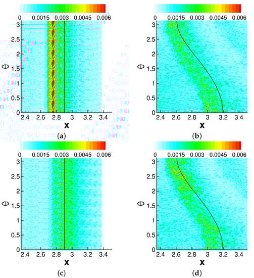
Figure 21.
Wall-pressure coefficient Fourier amplitudes for axisymmetric (left) and asymmetric (right) case. Modes (a) (), (b) (), (c) (), and (d) (). The shock impingement line is marked by the black line.
4.5.2. Probability Density Function of Axial Skin-Friction Coefficient
To more quantitatively assess the amount of time the flow is separated, the probability density function (PDF) of flow separation was computed from the axial skin-friction coefficient (Figure 22). Compared to the axisymmetric interaction (dashed line in figure), for the asymmetric interaction the flow is on average less separated (lower PDF) but the region of intermittent separation extends over a larger downstream distance. This is consistent with the -distributions in Figure 17 which are spread over a larger downstream interval for the asymmetric case. Interestingly, for , which is a location with significant crossflow, the flow is intermittently separated, but the PDF is still lower than for and . For , intermittent flow separation also occurs near as a result of the secondary SBLI (also see Figure 12). In summary, sweep reduces the intermittency of flow separation and increases the downstream extent over which flow separation occurs.
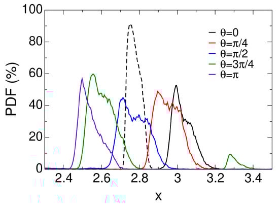
Figure 22.
Probability density function of flow separation for axisymmetric (dashed line) and asymmetric (solid lines) case.
4.5.3. Proper Orthogonal Decomposition of Pressure Coefficient
The POD technique [53] was used to analyze the same instantaneous wall-pressure data as in the previous Fourier analysis. The temporal averages were subtracted from the wall-pressure data prior to the POD analysis. Different from the Fourier analysis, the entire datasets were analyzed at once and not split up into 10 series. The POD eigenvalues for all modes (6780 modes for axisymmetric case and 4900 modes for asymmetric case) are presented in Figure 23. For the axisymmetric case, a small spectral gap after the first two modes suggests that they have more dynamic significance than the higher POD modes. Similar to Zuo et al. [54], who performed POD of both the streamwise velocity and wall-pressure fluctuations for a conical shock wave impinging on a flat plate, the eigenvalues decay smoothly towards the higher modes. The decay is faster for the axisymmetric case, meaning that the flow is less chaotic (or stochastic) than for the asymmetric case.
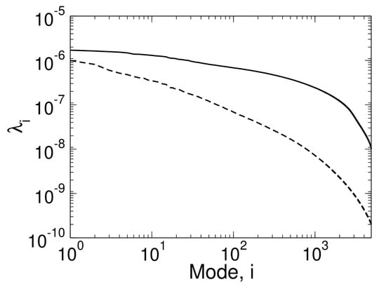
Figure 23.
Wall-pressure coefficient POD eigenvalues for axisymmetric (dashed line) and asymmetric (solid line) case.
Figure 24 shows spectra of the time-coefficients for the four leading POD modes. As for the Fourier analysis, the Strouhal number was based on the upstream boundary layer thickness. For the axisymmetric interaction, modes 1 and 2 have appreciable amplitudes near . Modes 3 and 4 have peaks near , and (also see Figure 21c). For the asymmetric case, the low-frequency content is suppressed compared to the axisymmetric interaction. This is in agreement with the present Fourier analysis (Figure 21) and with Lee and Gross [18], who reported a suppression of the low-frequency unsteadiness for infinite swept interactions. Mode 1 has a maximum at (also see Figure 21b), modes 1 and 2 have maxima at (also see Figure 21d) and modes 2, 3, and 4 have maxima near .
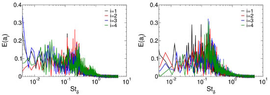
Figure 24.
Fourier transforms of POD time coefficients for axisymmetric (left) and asymmetric (right) case.
Figure 25 displays visualizations of the first four POD modes. For both cases, modes 1 and 2 and modes 3 and 4 form mode pairs. Mode pairs are characterized by similar eigenvalue magnitudes, as well as similar time-coefficients and mode shapes that are shifted by a quarter wavelength relative to each other. For the axisymmetric interaction, modes 1 and 2 capture traveling spanwise coherent structures. For the asymmetric interaction, modes 1 and 2 capture spanwise structures predominantly near but to a lesser extent also near , both regions which little no or little crossflow. This indicates that the unsteadiness is linked to the amount of flow separation (compare to Figure 12). Modes 3 and 4 for the axisymmetric interaction represent a mix of 2D and 3D waves that is characterized by three dominant frequencies (also see Figure 24). Based on earlier research, it may be speculated that the 3D component is related to the low-frequency unsteadiness [55] and that the 2D component is related to the mid-frequency unsteadiness. For the asymmetric interaction, modes 3 and 4 appear to capture a 3D modulation of the spanwise structures near .
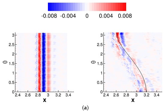
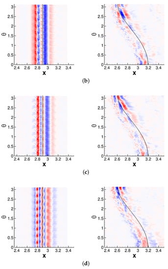
Figure 25.
POD modes (a) , (b) , (c) , and (d) for axisymmetric (left) and asymmetric (right) case.
5. Discussion
Reynolds-averaged Navier–Stokes (RANS) calculations are routinely used for designing and analyzing inlet flows. Government labs and industry are interested in assessing the suitability of higher fidelity methods, such as large-eddy simulations (LES) for the analysis of inlet flows. This motivated researchers at NASA Glenn Research Center (GRC) to design a canonical Mach 2.5 turbulent shock wave boundary layer interaction (SBLI) experiment with axisymmetric test section [28,32,35] for validating turbulence models and large eddy simulations (LES). Different from 2D wind tunnel experiments with planar interactions, the experiment does not suffer from endwall effects.
For the original series of experiments, the shock generator was placed on the centerline of the test section [28]. Wall-resolved implicit LES (ILES) for this concentric arrangement with nominally axisymmetric 2D SBLI were performed by Mosele et al. [37]. For these simulations, symmetry could be exploited and the azimuthal extent of the computational domain was 20 deg. To lower the computational expense of the simulations, the Reynolds number was reduced by a factor of 10 compared to the experiments. In later experiments [32,35], the shock generator was then displaced from the centerline to obtain asymmetric interactions. Two different shock generator offsets from the centerline, and , were considered, where R is the test section radius. Simulations of the asymmetric interactions require computational domains with an azimuthal extent of 180 deg. This strains computational resources and led to the decision to only perform one ILES (at 10 times lower Reynolds number) for the larger shock generator offset () for which the flow asymmetry is more pronounced. The initial and boundary conditions for the ILES were obtained from precursor RANS calculations.
The results obtained from the present ILES for the asymmetric interaction are compared with results from the earlier ILES [37] for the axisymmetric interaction. Concerning the mean flow, the amount of flow separation is considerably reduced for the asymmetric interaction compared to the axisymmetric interaction. The pressure increase across the SBLI is stronger on the side that is closest to the shock generator and this results in a strong crossflow away from the high-pressure region, which suppresses the mean separation. Nevertheless, probability density functions of the amount of flow separation suggest intermittent flow separation even for the region with strong crossflow. Fourier-spectra of the wall-pressure coefficient reveal low- and mid-frequency unsteadiness for the axisymmetric interaction. For the asymmetric interactions, the unsteadiness is concentrated near the two regions where the flow is separated in the mean (closest and farthest from shock generator) and the low-frequency unsteadiness appears suppressed in agreement with LES for an infinite swept interaction by Lee and Gross [18]. These finding are corroborated by a proper orthogonal decomposition (POD) of the wall-pressure coefficient. For the axisymmetric interaction, the POD captures pronounced mid-frequency shedding of spanwise coherent structures and mixed modes (low- and mid-frequencies) with 2D and 3D component. For the asymmetric interaction, the POD captures mid-frequency structures for the two regions where the flow is separated in the mean.
In summary, the current study demonstrates that incorporating sweep in cylindrical inlets with conical shock waves mitigates flow separation and reduces unsteady flow effects. Moreover, as the degree of asymmetry increases, the impact of these effects becomes less pronounced. The present results suggest that the low-frequency unsteadiness, which is of concern to structural designers, may be less of a factor for swept interactions. A detailed parameter study, that covers a broader range of Mach numbers, shock strengths, and sweep angles, would be required to discover trends and provide quantitative guidance to the designers of supersonic engine inlets. Future efforts will concentrate on employing hybrid turbulence modeling approaches, such as the delayed detached-eddy simulations [56], to simulate entire inlet flows at higher Reynolds numbers.
Author Contributions
Conceptualization, J.-P.M., A.G., and J.S.; methodology, J.-P.M., A.G.; software, A.G.; validation, J.-P.M.; formal analysis, J.-P.M.; investigation, J.-P.M.; writing—original draft preparation, J.-P.M.; writing—review and editing, A.G., and J.S.; visualization, J.-P.M.; supervision, A.G. and J.S.; project administration, A.G. and J.S.; funding acquisition, A.G. and J.S. All authors have read and agreed to the published version of the manuscript.
Funding
This material is based upon work supported by the National Aeronautics and Space Administration under grant 80NSSC19K1675 issued through the NASA Shared Services Center. The NASA High-End Computing (HEC) Program through the NASA Advanced Supercomputing (NAS) Division at Ames Research Center provided the computational resources for this work.
Conflicts of Interest
The authors declare no conflict of interest.
Nomenclature
| ai | Time coefficient |
| Cf | Skin-friction coefficient |
| Cp | Pressure coefficient |
| D | Test section diameter |
| E | Amplitude |
| f | Frequency |
| H | Shape factor |
| k | Turbulent kinetic energy |
| M | Mach number |
| n | Fourier mode number |
| p | Pressure |
| Pr | Prandtl number |
| Re | Reynolds number |
| rSG | Shock generator centerbody radius |
| St | Strouhal number |
| t | Time |
| T | Temperature |
| vx,vr,vt | Velocities |
| r,θ,x | Cylindrical coordinates |
| Greek Symbols | |
| α | Shock generator cone half-angle |
| γ | Ratio of specific heats |
| δ | Boundary layer thickness |
| δ∗ | Displacement thickness |
| ε | turbulent dissipation rate |
| ϑ | momentum thickness |
| λ | Eigenvalue |
| μ | Dynamic viscosity |
| v | Kinematic viscosity |
| ρ | Density |
| Subscripts | |
| i | POD mode number |
| incomp | Incompressible |
| rms | Root-mean-square |
| ∞ | Approach flow freestream conditions |
| Superscripts | |
| + | In wall units |
| * | Dimensional quantity |
| ’ | Fluctuation |
References
- Clemens, N.T.; Narayanaswamy, V. Low-Frequency Unsteadiness of Shock Wave/Turbulent Boundary Layer Interactions. Annu. Rev. Fluid Mech. 2014, 46, 469–492. [Google Scholar] [CrossRef]
- Piponniau, S.; Dussauge, J.P.; Debieve, J.F.; Dupont, P. A simple model for low-frequency unsteadiness in shock-induced separation. J. Fluid Mech. 2009, 629, 87–108. [Google Scholar] [CrossRef]
- Gaitonde, D.V. Progress in shock wave/boundary layer interactions. Prog. Aerosp. Sci. 2015, 72, 80–99. [Google Scholar] [CrossRef]
- Agostini, L.; Larchevêque, L.; Dupont, P. Mechanism of shock unsteadiness in separated shock/boundary-layer interactions. Phys. Fluids 2015, 27, 126103. [Google Scholar] [CrossRef]
- Touber, E.; Sandham, N.D. Large-eddy simulation of low-frequency unsteadiness in a turbulent shock-induced separation bubble. Theor. Comput. Fluid Dyn. 2009, 23, 79–107. [Google Scholar] [CrossRef]
- Threadgill, J.A.; Little, J.C. An inviscid analysis of swept oblique shock reflections. J. Fluid Mech. 2020, 890, A22. [Google Scholar] [CrossRef]
- Dussauge, J.P.; Dupont, P.; Debiève, J.F. Unsteadiness in shock wave boundary layer interactions with separation. Aerosp. Sci. Technol. 2006, 10, 85–91. [Google Scholar] [CrossRef]
- Ganapathisubramani, B.; Clemens, N.; Dolling, D. Effects of upstream boundary layer on the unsteadiness of shock-induced separation. J. Fluid Mech. 2007, 585, 369–394. [Google Scholar] [CrossRef]
- Priebe, S.; Tu, J.H.; Rowley, C.W.; Martín, M.P. Low-frequency dynamics in a shock-induced separated flow. J. Fluid Mech. 2016, 807, 441–477. [Google Scholar] [CrossRef]
- Gaitonde, D.V.; Adler, M.C. Dynamics of Three-Dimensional Shock-Wave/Boundary-Layer Interactions. Annu. Rev. Fluid Mech. 2023, 55, 291–321. [Google Scholar] [CrossRef]
- Panaras, A.G. Review of the physics of swept-shock/boundary layer interactions. Prog. Aerosp. Sci. 1996, 32, 173–244. [Google Scholar] [CrossRef]
- Erengil, M.E.; Dolling, D.S. Effects of Sweepback on Unsteady Separation in Mach 5 Compression Ramp Interactions. AIAA J. 1993, 31, 302–311. [Google Scholar] [CrossRef]
- Settles, G.S.; Teng, H.Y. Cylindrical and Conical Flow Regimes of Three-Dimensional Shock/Boundary-Layer Interactions. AIAA J. 1984, 22, 194–200. [Google Scholar] [CrossRef]
- Vanstone, L.; Musta, M.N.; Seckin, S.; Clemens, N. Experimental study of the mean structure and quasi-conical scaling of a swept-compression-ramp interaction at Mach 2. J. Fluid Mech. 2018, 841, 1–27. [Google Scholar] [CrossRef]
- Huang, X.; Estruch-Samper, D. Low-frequency unsteadiness of swept shock-wave/turbulent-boundary-layer interaction. J. Fluid Mech. 2018, 856, 797–821. [Google Scholar] [CrossRef]
- Arora, N.; Mears, L.; Alvi, F.S. Unsteady Characteristics of a Swept-Shock/Boundary-Layer Interaction at Mach 2. AIAA J. 2019, 57, 4548–4559. [Google Scholar] [CrossRef]
- Adler, M.C.; Gaitonde, D.V. Dynamics of strong swept-shock/turbulent-boundary-layer interactions. J. Fluid Mech. 2020, 896, A29. [Google Scholar] [CrossRef]
- Lee, S.; Gross, A. Numerical Investigation of Sweep Effect on Turbulent Shock-Wave Boundary-Layer Interaction. AIAA J. 2022, 60, 712–730. [Google Scholar] [CrossRef]
- Fang, J.; Yao, Y.; Zheltovodov, A.A.; Lu, L. Investigation of Three-Dimensional Shock Wave/Turbulent-Boundary-Layer Interaction Initiated by a Single Fin. AIAA J. 2017, 55, 509–523. [Google Scholar] [CrossRef]
- Mears, L.J.; Baldwin, A.; Ali, M.Y.; Kumar, R.; Alvi, F.S. Spatially resolved mean and unsteady surface pressure in swept SBLI using PSP. Exp. Fluids 2020, 61, 92. [Google Scholar] [CrossRef]
- Baldwin, A.; Mears, L.J.; Kumar, R.; Alvi, F.S. Effects of Reynolds Number on Swept Shock-Wave/Boundary-Layer Interactions. AIAA J. 2021, 59, 3883–3899. [Google Scholar] [CrossRef]
- Vanstone, L.; Clemens, N.T. Proper Orthogonal Decomposition Analysis of Swept-Ramp Shock-Wave/Boundary-Layer Unsteadiness at Mach 2. AIAA J. 2019, 57, 3395–3409. [Google Scholar] [CrossRef]
- Adler, M.C.; Gaitonde, D.V. Flow Similarity in Strong Swept-Shock/Turbulent-Boundary-Layer Interactions. AIAA J. 2019, 57, 1579–1593. [Google Scholar] [CrossRef]
- Padmanabhan, S.; Maldonado, J.C.; Threadgill, J.A.; Little, J.C. Experimental Study of Swept Impinging Oblique Shock/Boundary-Layer Interactions. AIAA J. 2021, 59, 140–149. [Google Scholar] [CrossRef]
- Mears, L.J.; Sellappan, P.; Alvi, F.S. Three-Dimensional Flowfield in a Fin-Generated Shock Wave/Boundary-Layer Interaction Using Tomographic PIV. AIAA J. 2021, 59, 4869–4880. [Google Scholar] [CrossRef]
- Zuo, F.Y.; Memmolo, A.; Huang, G.p.; Pirozzoli, S. Direct numerical simulation of conical shock wave–turbulent boundary layer interaction. J. Fluid Mech. 2019, 877, 167–195. [Google Scholar] [CrossRef]
- Kussoy, M.; Viegas, J.; Horstman, C. Investigation of a Three-Dimensional Shock Wave Separated Turbulent Boundary Layer. AIAA J. 1980, 18, 1477–1484. [Google Scholar] [CrossRef]
- Davis, D.O. CFD Validation Experiment of a Mach 2.5 Axisymmetric Shock-Wave/Boundary-Layer Interaction. In Proceedings of the Fluids Engineering Division Summer Meeting. American Society of Mechanical Engineers, Seoul, Republic of Korea, 26–31 July 2015; Volume 57212, p. V001T06A001. [Google Scholar]
- Bruce, P.; Burton, D.; Titchener, N.; Babinsky, H. Corner effect and separation in transonic channel flows. J. Fluid Mech. 2011, 679, 247–262. [Google Scholar] [CrossRef]
- Burton, D.; Babinsky, H. Corner separation effects for normal shock wave/turbulent boundary layer interactions in rectangular channels. J. Fluid Mech. 2012, 707, 287–306. [Google Scholar] [CrossRef]
- Chou, J.H.; Childs, M.E.; Wong, R.S. An Experimental Study of Three-Dimensional Shock Wave/Turbulent Boundary Layer Interactions in a Supersonic Flow. In Proceedings of the 18th Fluid Dynamics and Plasmadynamics and Lasers Conference, Cincinnati, OH, USA, 16–18 July 1985; AIAA Paper 1985-1556. AIAA: Reston, VA, USA, 1985. [Google Scholar]
- Sasson, J.; Reising, H.H.; Davis, D.O.; Barnhart, P.J. Summary of Shock Wave Turbulent Boundary Layer Interaction Experiments In a Circular Test Section; AIAA Paper 2023-0442; AIAA: Reston, VA, USA, 2023. [Google Scholar]
- Settles, G.S.; Dodson, L.J. Supersonic and Hypersonic Shock/Boundary-Layer Interaction Database. AIAA J. 1994, 32, 1377–1383. [Google Scholar] [CrossRef]
- Sasson, J. Conical Shock Wave Turbulent Boundary Layer Interactions in a Circular Test Section at Mach 2.5. Ph.D. Thesis, Case Western Reserve University, Cleveland, OH, USA, 2022. [Google Scholar]
- Sasson, J.; Barnhart, P. Spectral Analysis of a Shock Wave Turbulent Boundary Layer Interaction In a Circular Test Section. In Proceedings of the AIAA SCITECH 2023 Forum, National Harbor, MD, USA, 23–27 January 2023; AIAA Paper 2023-2255. AIAA: Reston, VA, USA, 2023. [Google Scholar]
- Reising, H.H.; Davis, D.O. Development and Assessment of a New Particle Image Velocimetry System in the NASA GRC 225 cm2 Wind Tunnel. In Proceedings of the AIAA SCITECH 2023 Forum, National Harbor, MD, USA, 23–27 January 2023; AIAA Paper 2023-0631. AIAA: Reston, VA, USA, 2023. [Google Scholar]
- Mosele, J.P.; Gross, A.; Slater, J. Numerical Investigation of Mach 2.5 Axisymmetric Turbulent Shock Wave Boundary Layer Interactions. Aerospace 2023, 10, 159. [Google Scholar] [CrossRef]
- Souverein, L.; Bakker, P.; Dupont, P. A scaling analysis for turbulent shock-wave/boundary-layer interactions. J. Fluid Mech. 2013, 714, 505–535. [Google Scholar] [CrossRef]
- Gross, A.; Fasel, H.F. High-Order Accurate Numerical Method for Complex Flows. AIAA J. 2008, 46, 204–214. [Google Scholar] [CrossRef]
- Gross, A.; Fasel, H.F. Numerical investigation of supersonic flow for axisymmetric cones. Math. Comput. Simul. 2010, 81, 133–142. [Google Scholar] [CrossRef]
- Wilcox, D.C. Turbulence Modeling for CFD, 3rd ed.; DCW Industries: New York, NY, USA, 2006. [Google Scholar]
- Wilcox, D.C. Formulation of the k-w Turbulence Model Revisited. AIAA J. 2008, 46, 2823–2838. [Google Scholar] [CrossRef]
- Carr, J.C.; Beatson, R.K.; Cherrie, J.B.; Mitchell, T.J.; Fright, W.R.; McCallum, B.C.; Evans, T.R. Reconstruction and Representation of 3D Objects with Radial Basis Functions. In Proceedings of the 28th Annual Conference on Computer Graphics and Interactive Techniques, Los Angeles, CA, USA, 12–17 August 2001; pp. 67–76. [Google Scholar]
- Poletto, R.; Craft, T.; Revell, A. A New Divergence Free Synthetic Eddy Method for the Reproduction of Inlet Flow Conditions for LES. Flow Turbul. Combust. 2013, 91, 519–539. [Google Scholar] [CrossRef]
- Lumley, J.L. The structure of inhomogeneous turbulent flows. In Atmospheric Turbulence and Radio Wave Propagation; National Institute of Informatics: Tokyo, Japan, 1967. [Google Scholar]
- Gross, A.; Lee, S. Numerical analysis of laminar and turbulent shock-wave boundary layer interactions. In Proceedings of the 2018 Fluid Dynamics Conference, Atlanta, GA, USA, 25–29 June 2018; AIAA Paper 2018-4033. AIAA: Reston, VA, USA, 2018. [Google Scholar]
- Sirovich, L. Turbulence and the Dynamics of Coherent Structures. Quaterly Appl. Math. 1987, 45, 561–590. [Google Scholar] [CrossRef]
- Hunt, J.; Wray, A.; Moin, P. Eddies, stream, and convergence zones in turbulent flows. In Studying Turbulence Using Numerical Simulation Databases, 2. Proceedings of the 1988 Summer Program; Center for Turbulence Research: Stanford, CA, USA, 1988; Volume 193. [Google Scholar]
- Anderson, J.D. Modern Compressible Flow: With Historical Perspective; McGraw-Hill: New York, NY, USA, 1990; Volume 12. [Google Scholar]
- Tobak, M.; Peake, D.J. Topology of three-dimensional separated flows. Annu. Rev. Fluid Mech. 1982, 14, 61–85. [Google Scholar] [CrossRef]
- Adler, M.C.; Gaitonde, D.V. Unsteadiness in swept-compression-ramp shock/turbulent-boundary-layer interactions. In Proceedings of the 55th AIAA Aerospace Sciences Meeting, Grapevine, TX, USA, 9–13 January 2017; AIAA Paper 2017-0987. AIAA: Reston, VA, USA, 2017. [Google Scholar]
- Arora, N.; Ali, M.Y.; Zhang, Y.; Alvi, F.S. Flowfield Measurements in a Mach 2 Fin-Generated Shock/Boundary-Layer Interaction. AIAA J. 2018, 56, 3963–3974. [Google Scholar] [CrossRef]
- Berkooz, G.; Holmes, P.; Lumley, J.L. The proper orthogonal decomposition in the analysis of turbulent flows. Annu. Rev. Fluid Mech. 1993, 25, 539–575. [Google Scholar] [CrossRef]
- Zuo, F.Y.; Yu, M.; Pirozzoli, S. Modal Analysis of Separation Bubble Unsteadiness in Conical Shock Wave/Turbulent Boundary Layer Interaction. AIAA J. 2022, 60, 5123–5135. [Google Scholar] [CrossRef]
- Gross, A.; Little, J.; Fasel, H.F. Numerical investigation of unswept and swept turbulent shock-wave boundary layer interactions. Aerosp. Sci. Technol. 2022, 123, 107455. [Google Scholar] [CrossRef]
- Mosele, J.P.G.; Gross, A.; Slater, J.W. Numerical Investigation of Flow Over Periodic Hill. In Proceedings of the AIAA AVIATION 2022 Forum, Gravesend, UK, 27 June–20 July 2022; AIAA Paper 2022-3228. AIAA: Reston, VA, USA, 2022. [Google Scholar]
Disclaimer/Publisher’s Note: The statements, opinions and data contained in all publications are solely those of the individual author(s) and contributor(s) and not of MDPI and/or the editor(s). MDPI and/or the editor(s) disclaim responsibility for any injury to people or property resulting from any ideas, methods, instructions or products referred to in the content. |
© 2023 by the authors. Licensee MDPI, Basel, Switzerland. This article is an open access article distributed under the terms and conditions of the Creative Commons Attribution (CC BY) license (https://creativecommons.org/licenses/by/4.0/).