Integrating Urban Form, Function, and Energy Fluxes in a Heat Exposure Indicator in View of Intra-Urban Heat Island Assessment and Climate Change Adaptation


Abstract
1. Introduction
- High values of the ratio of building’s height (H) to street width (W)—canyon aspect ratio (H/W)—result in canyon trapping [39,40], i.e., the absorption of shortwave radiation in the canopy is stronger via multiple reflections on walls, and in the longwave radiant heat loss being strongly obscured [41,42].
- Sensible heat refers to the direct warming of air that can be sensed by a thermometer, whereas the latent heat component of the urban energy balance is mostly associated with the energy exchanges during surface moisture evaporation. The dry, impermeable urban facets favor sensible (QH) over latent (QE) heat flux; i.e., the Bowen ratio (β = QH/QE) has higher values. As a result, the evaporative cooling effect decreases [43,44].
- High thermal inertia of the construction materials and of the built environment in general results in a large proportion of incoming solar radiation to be stored during the daytime in the urban system—high net heat storage (ΔQS)—and being released at nighttime, maintaining the urban heating effect [45].
- The anthropogenic heat flux (QF), e.g., waste heat from vehicular traffic and from space heating/cooling, is an additional energy source into the surface energy balance [46].
2. Materials and Methods
2.1. Study Area
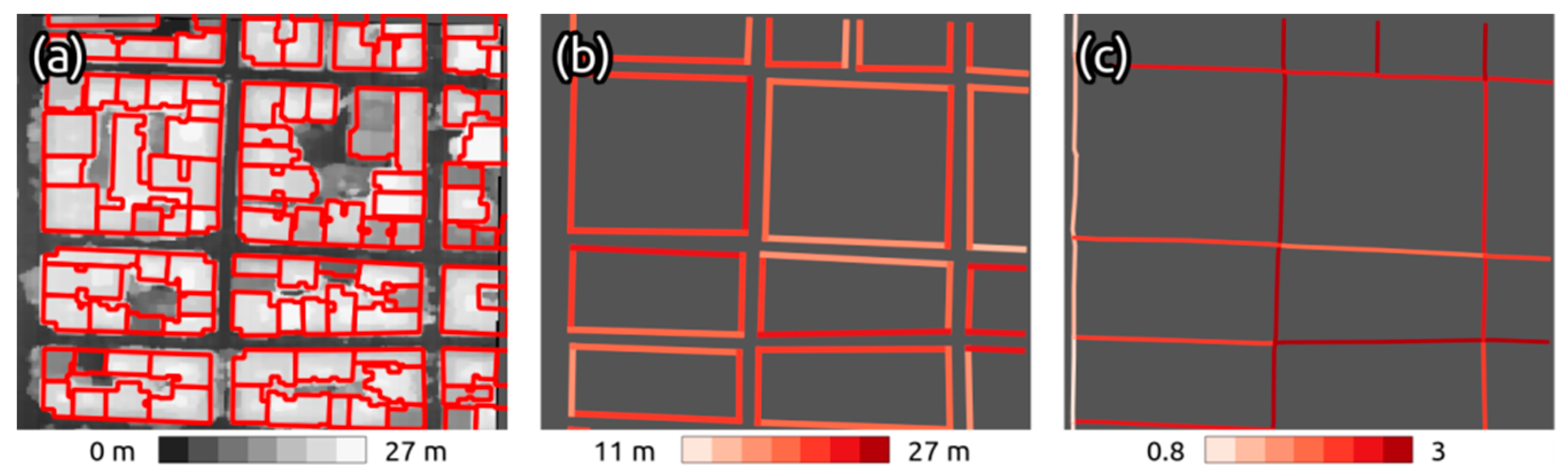
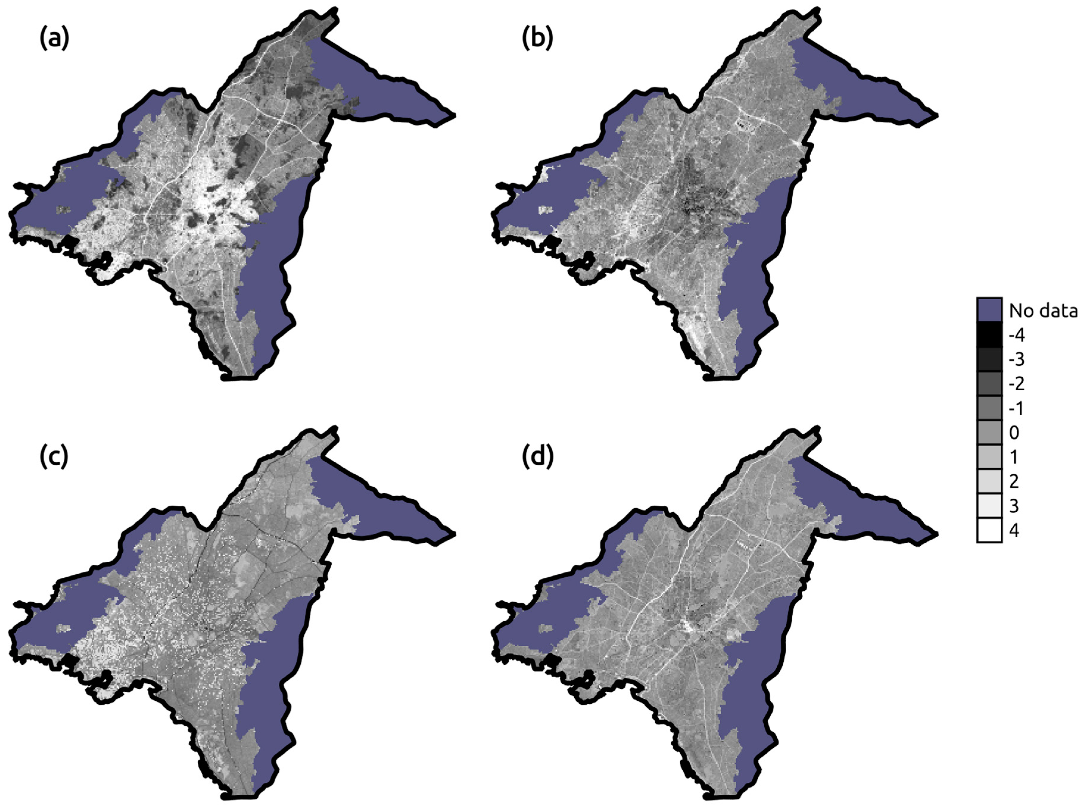
2.2. Urban Form
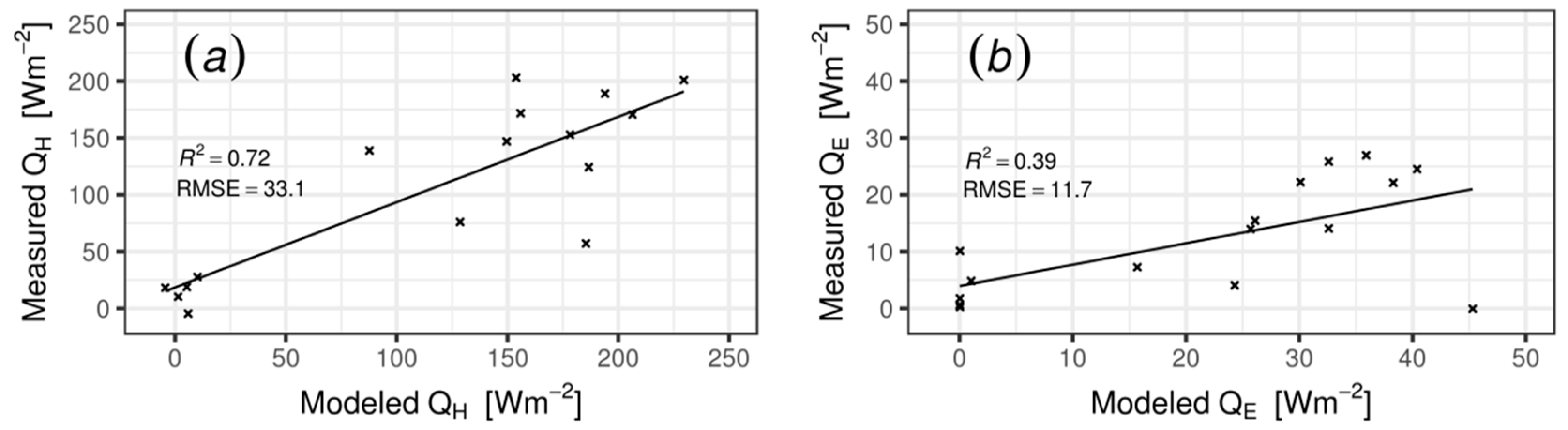
2.3. Bowen Ratio
2.4. Net Storage Heat Flux
2.5. Anthropogenic Heat Flux
2.5.1. Building Heat Emissions (QFB)
2.5.2. Vehicular Heat Emissions (QFV)
2.5.3. Metabolic heat emissions (QFM)
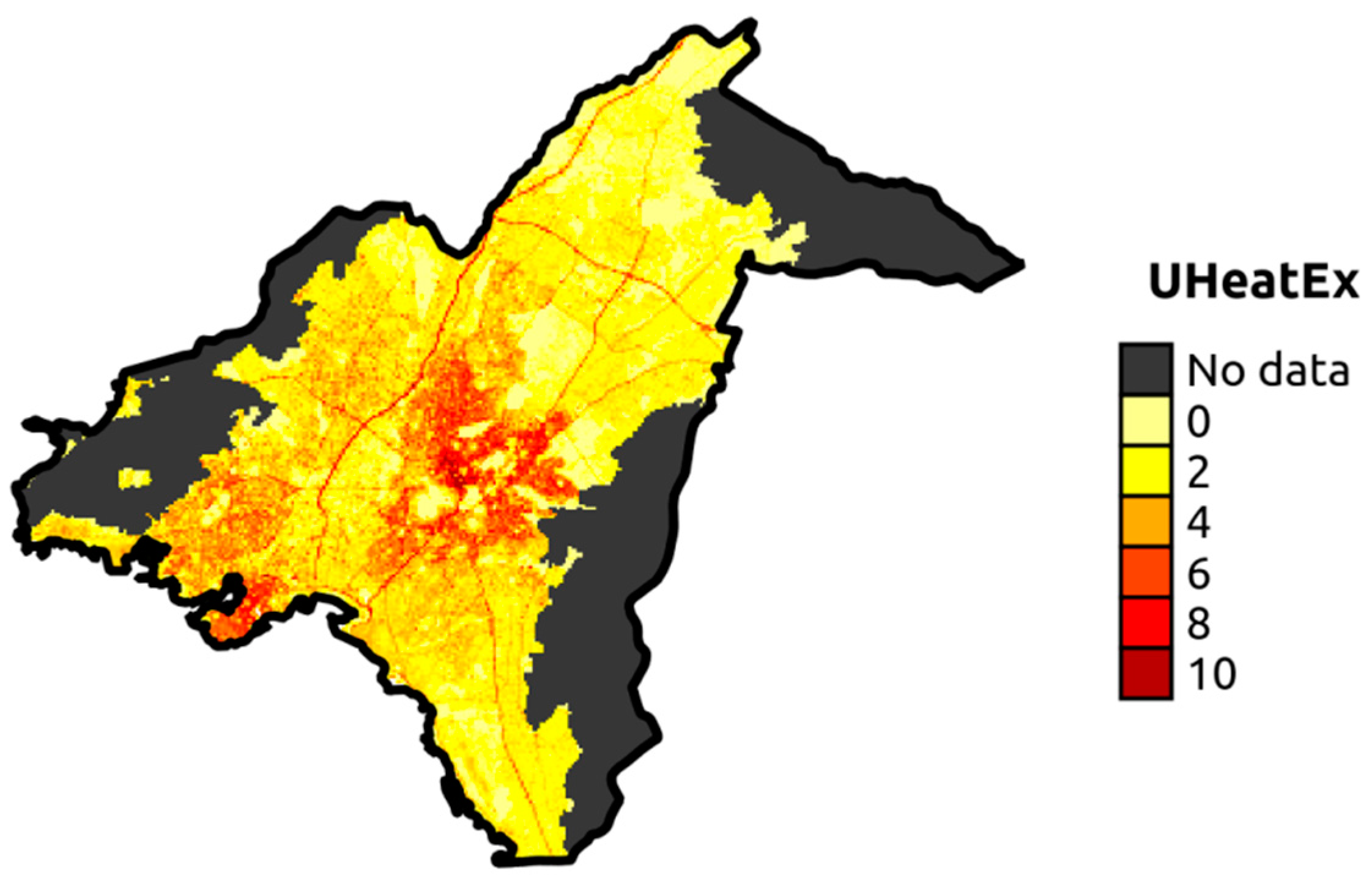
2.6. UHeatEx
2.7. Local Climate Zones
2.8. Climate Change Projections
3. Results
4. Discussion
5. Conclusions
Author Contributions
Funding
Acknowledgments
Conflicts of Interest
References
- United Nations. Press Release of the World Urbanization Prospects 2018; United Nations: New York, NY, USA, 2018. [Google Scholar]
- Oke, T.R. The energetic basis of the urban heat island. Q. J. R. Meteorol. Soc. 1982, 108, 1–24. [Google Scholar] [CrossRef]
- Oke, T.R.; Mills, G.; Christen, A.; Voogt, J.A. Urban Climates; Cambridge University Press: Cambridge, UK, 2017. [Google Scholar]
- Fortuniak, K.; Kłysik, K.; Wibig, J. Urban–rural contrasts of meteorological parameters in Łódź. Theor. Appl. Climatol. 2006, 84, 91–101. [Google Scholar] [CrossRef]
- Van Hove, L.W.A.; Jacobs, C.M.J.; Heusinkveld, B.G.; Elbers, J.A.; van Driel, B.L.; Holtslag, A.A.M. Temporal and spatial variability of urban heat island and thermal comfort within the Rotterdam agglomeration. Build. Environ. 2015, 83, 91–103. [Google Scholar] [CrossRef]
- Skarbit, N.; Stewart, I.D.; Unger, J.; Gál, T. Employing an urban meteorological network to monitor air temperature conditions in the ‘local climate zones’ of Szeged, Hungary. Int. J. Climatol. 2017, 37, 582–596. [Google Scholar] [CrossRef]
- Keramitsoglou, I.; Kiranoudis, C.T.; Ceriola, G.; Weng, Q.; Rajasekar, U. Identification and analysis of urban surface temperature patterns in Greater Athens, Greece, using MODIS imagery. Remote Sens. Environ. 2011, 115, 3080–3090. [Google Scholar] [CrossRef]
- Parlow, E.; Vogt, R.; Feigenwinter, C. The urban heat island of Basel—Seen from different perspectives. Die Erde J. Geogr. Soc. Berl. 2014, 145, 96–110. [Google Scholar]
- Bonafoni, S.; Anniballe, R.; Pichierri, M. Comparison between surface and canopy layer urban heat island using MODIS data. In Proceedings of the 2015 Joint Urban Remote Sensing Event (JURSE), Lausanne, Switzerland, 30 March–1 April 2015; pp. 1–4. [Google Scholar]
- Santamouris, M.; Cartalis, C.; Synnefa, A.; Kolokotsa, D. On the impact of urban heat island and global warming on the power demand and electricity consumption of buildings—A review. Energy Build. 2015, 98, 119–124. [Google Scholar] [CrossRef]
- Magli, S.; Lodi, C.; Lombroso, L.; Muscio, A.; Teggi, S. Analysis of the urban heat island effects on building energy consumption. Int. J. Energy Environ. Eng. 2015, 6, 91–99. [Google Scholar] [CrossRef]
- Zanobetti, A.; Schwartz, J. Temperature and mortality in nine US cities. Epidemiology 2008, 19, 563–570. [Google Scholar] [CrossRef]
- Pyrgou, A.; Santamouris, M. Increasing probability of heat-related mortality in a Mediterranean city due to urban warming. Int. J. Environ. Res. Public Health 2018, 15, 1571. [Google Scholar] [CrossRef]
- Nastos, P.T.; Matzarakis, A. The effect of air temperature and human thermal indices on mortality in Athens, Greece. Theor. Appl. Climatol. 2012, 108, 591–599. [Google Scholar] [CrossRef]
- Heaviside, C.; Tsangari, H.; Paschalidou, A.; Vardoulakis, S.; Kassomenos, P.; Georgiou, K.E.; Yamasaki, E.N. Heat-related mortality in Cyprus for current and future climate scenarios. Sci. Total Environ. 2016, 569–570, 627–633. [Google Scholar] [CrossRef] [PubMed]
- Fouillet, A.; Rey, G.; Laurent, F.; Pavillon, G.; Bellec, S.; Guihenneuc-Jouyaux, C.; Clavel, J.; Jougla, E.; Hémon, D. Excess mortality related to the August 2003 heat wave in France. Int. Arch. Occup. Environ. Health 2006, 80, 16–24. [Google Scholar] [CrossRef] [PubMed]
- Kosatsky, T.; Henderson, S.B.; Pollock, S.L. Shifts in Mortality during a Hot Weather Event in Vancouver, British Columbia: Rapid Assessment with Case-Only Analysis. Am. J. Public Health 2012, 102, 2367–2371. [Google Scholar] [CrossRef] [PubMed]
- Stocker, T. Climate Change 2013: The Physical Science Basis: Working Group I Contribution to the Fifth Assessment Report of the Intergovernmental Panel on Climate Change; Cambridge University Press: Cambridge, UK, 2014. [Google Scholar]
- Rosenzweig, C.; Solecki, W.D.; Hammer, S.A.; Mehrotra, S. Climate Change and Cities: First Assessment Report of the Urban Climate Change Research Network; Cambridge University Press: Cambridge, UK, 2011. [Google Scholar]
- Shonkoff, S.B.; Morello-Frosch, R.; Pastor, M.; Sadd, J. The climate gap: Environmental health and equity implications of climate change and mitigation policies in California—A review of the literature. Clim. Chang. 2011, 109, 485–503. [Google Scholar] [CrossRef]
- Grineski, S.E.; Collins, T.W.; Ford, P.; Fitzgerald, R.; Aldouri, R.; Velázquez-Angulo, G.; de Lourdes Romo Aguilar, M.; Lu, D. Climate change and environmental injustice in a bi-national context. Appl. Geogr. 2012, 33, 25–35. [Google Scholar] [CrossRef]
- Mitchell, B.C.; Chakraborty, J. Landscapes of thermal inequity: Disproportionate exposure to urban heat in the three largest US cities. Environ. Res. Lett. 2015, 10, 115005. [Google Scholar] [CrossRef]
- Voelkel, J.; Hellman, D.; Sakuma, R.; Shandas, V. Assessing Vulnerability to Urban Heat: A Study of Disproportionate Heat Exposure and Access to Refuge by Socio-Demographic Status in Portland, Oregon. Int. J. Environ. Res. Public Health 2018, 15, 640. [Google Scholar] [CrossRef]
- Ren, C.; Lau, K.L.; Yiu, K.P.; Ng, E. The application of urban climatic mapping to the urban planning of high-density cities: The case of Kaohsiung, Taiwan. Cities 2013, 31, 1–16. [Google Scholar] [CrossRef]
- Stewart, I.D.; Oke, T.R. Local Climate Zones for Urban Temperature Studies. Bull. Am. Meteorol. Soc. 2012, 93, 1879–1900. [Google Scholar] [CrossRef]
- Alexander, P.J.; Mills, G. Local Climate Classification and Dublin’s Urban Heat Island. Atmosphere 2014, 5, 755–774. [Google Scholar] [CrossRef]
- Arnds, D.; Böhner, J.; Bechtel, B. Spatio-temporal variance and meteorological drivers of the urban heat island in a European city. Theor. Appl. Climatol. 2017, 128, 43–61. [Google Scholar] [CrossRef]
- Kaloustian, N.; Bechtel, B. Local Climatic Zoning and Urban Heat Island in Beirut. Procedia Eng. 2016, 169, 216–223. [Google Scholar] [CrossRef]
- Stewart, I.D. A systematic review and scientific critique of methodology in modern urban heat island literature. Int. J. Climatol. 2011, 31, 200–217. [Google Scholar] [CrossRef]
- Fenner, D.; Meier, F.; Bechtel, B.; Otto, M.; Scherer, D. Intra and inter ‘local climate zone’ variability of air temperature as observed by crowdsourced citizen weather stations in Berlin, Germany. Meteorol. Z. 2017, 26, 525–547. [Google Scholar] [CrossRef]
- Quanz, J.A.; Ulrich, S.; Fenner, D.; Holtmann, A.; Eimermacher, J. Micro-Scale Variability of Air Temperature within a Local Climate Zone in Berlin, Germany, during Summer. Climate 2018, 6, 5. [Google Scholar] [CrossRef]
- Bechtel, B.; Alexander, P.J.; Beck, C.; Böhner, J.; Brousse, O.; Ching, J.; Demuzere, M.; Fonte, C.; Gál, T.; Hidalgo, J.; et al. Generating WUDAPT Level 0 data—Current status of production and evaluation. Urban Clim. 2019, 27, 24–45. [Google Scholar] [CrossRef]
- Wicki, A.; Parlow, E. Attribution of local climate zones using a multitemporal land use/land cover classification scheme. J. Appl. Remote Sens. 2017, 11, 026001. [Google Scholar] [CrossRef]
- Ng, E.; Ren, C.; Katzschner, L.; Yau, R. Urban climatic studies for hot and humid tropical coastal city of Hong Kong. In Proceedings of the 5th Japanese-German Meeting on Urban Climatology, Freiburg, Germany, 6–8 October 2008; p. 265. [Google Scholar]
- Smith, C.; Cavan, G.; Lindley, S. Urban climatic map studies in UK: Greater Manchester. In The Urban Climatic Map; Routledge: Abingdon, UK, 2015; pp. 313–326. [Google Scholar]
- Hu, X.; Xu, H. A new remote sensing index for assessing the spatial heterogeneity in urban ecological quality: A case from Fuzhou City, China. Ecol. Indic. 2018, 89, 11–21. [Google Scholar] [CrossRef]
- Alavipanah, S.; Schreyer, J.; Haase, D.; Lakes, T.; Qureshi, S. The effect of multi-dimensional indicators on urban thermal conditions. J. Clean. Prod. 2018, 177, 115–123. [Google Scholar] [CrossRef]
- Alavipanah, S.; Haase, D.; Lakes, T.; Qureshi, S. Integrating the third dimension into the concept of urban ecosystem services: A review. Ecol. Indic. 2017, 72, 374–398. [Google Scholar] [CrossRef]
- Aida, M. Urban albedo as a function of the urban structure—A model experiment. Bound. Layer Meteorol. 1982, 23, 405–413. [Google Scholar] [CrossRef]
- Krayenhoff, E.S.; Voogt, J.A. A microscale three-dimensional urban energy balance model for studying surface temperatures. Bound. Layer Meteorol. 2007, 123, 433–461. [Google Scholar] [CrossRef]
- Arnfield, A.J. Canyon geometry, the urban fabric and nocturnal cooling: A simulation approach. Phys. Geogr. 1990, 11, 220–239. [Google Scholar] [CrossRef]
- Voogt, J.A.; Oke, T.R. Validation of an urban canyon radiation model for nocturnal long-wave fluxes. Bound. Layer Meteorol. 1991, 54, 347–361. [Google Scholar] [CrossRef]
- Oke, T.R. The urban energy balance. Prog. Phys. Geogr. Earth Environ. 1988, 12, 471–508. [Google Scholar] [CrossRef]
- Ward, H.; Grimmond, C. Assessing the impact of changes in surface cover, human behaviour and climate on energy partitioning across Greater London. Landsc. Urban Plan. 2017, 165, 142–161. [Google Scholar] [CrossRef]
- Grimmond, C.S.B.; Oke, T.R. Heat Storage in Urban Areas: Local-Scale Observations and Evaluation of a Simple Model. J. Appl. Meteorol. 1999, 38, 922–940. [Google Scholar] [CrossRef]
- Sailor, D.J. A review of methods for estimating anthropogenic heat and moisture emissions in the urban environment. Int. J. Climatol. 2011, 31, 189–199. [Google Scholar] [CrossRef]
- Ferrante, A. Towards Nearly Zero Energy: Urban Settings in the Mediterranean Climate; Butterworth-Heinemann: Oxford, UK, 2016. [Google Scholar]
- Maloutas, T. Socio-economic segregation in Athens at the beginning of the twenty-first century. In Socio-Economic Segregation in European Capital Cities: East Meets West; Routledge: Abingdon, UK, 2015; pp. 156–185. [Google Scholar]
- Papamanolis, N. The main characteristics of the urban climate and the air quality in Greek cities. Urban Clim. 2015, 12, 49–64. [Google Scholar] [CrossRef]
- Papageorgiou, M.; Gemenetzi, G. Setting the grounds for the green infrastructure in the metropolitan areas of Athens and Thessaloniki: The role of green space. Eur. J. Environ. Sci. 2018, 8, 83–92. [Google Scholar] [CrossRef]
- Giannopoulou, K.; Livada, I.; Santamouris, M.; Saliari, M.; Assimakopoulos, M.; Caouris, Y.G. On the characteristics of the summer urban heat island in Athens, Greece. Sustain. Cities Soc. 2011, 1, 16–28. [Google Scholar] [CrossRef]
- Kourtidis, K.; Georgoulias, A.K.; Rapsomanikis, S.; Amiridis, V.; Keramitsoglou, I.; Hooyberghs, H.; Maiheu, B.; Melas, D. A study of the hourly variability of the urban heat island effect in the Greater Athens Area during summer. Sci. Total Environ. 2015, 517, 162–177. [Google Scholar] [CrossRef] [PubMed]
- Georgakis, C.; Santamouris, M. Determination of the Surface and Canopy Urban Heat Island in Athens Central Zone Using Advanced Monitoring. Climate 2017, 5, 97. [Google Scholar] [CrossRef]
- Copernicus Land Monitoring Service. Urban Atlas 2012. Available online: https://land.copernicus.eu/local/urban-atlas/urban-atlas-2012 (accessed on 14 March 2019).
- Agathangelidis, I.; Cartalis, C. Improving the disaggregation of MODIS land surface temperatures in an urban environment: A statistical downscaling approach using high-resolution emissivity. Int. J. Remote Sens. 2019, 40, 5261–5286. [Google Scholar] [CrossRef]
- Hellenic Statistical Authority (ELSTAT). Digital Cartographic Data. Available online: http://www.statistics.gr/en/digital-cartographical-data (accessed on 14 March 2019).
- OpenStreetMap Contributors. Planet Dump. Available online: https://planet.osm.org (accessed on 2 February 2019).
- Burian, S.J.; Velugubantla, S.P.; Brown, M.J. Morphological Analyses Using 3D Building Databases: Salt Lake City, Utah; LA-UR-02-6197, Los Alamos National Laboratory: Los Alamos, NM, USA, 2002. [Google Scholar]
- Jhaldiyal, A.; Gupta, K.; Gupta, P.K.; Thakur, P.; Kumar, P. Urban Morphology Extractor: A spatial tool for characterizing urban morphology. Urban Clim. 2018, 24, 237–246. [Google Scholar] [CrossRef]
- Lindberg, F.; Grimmond, C.S.B.; Martilli, A. Sunlit fractions on urban facets—Impact of spatial resolution and approach. Urban Clim. 2015, 12, 65–84. [Google Scholar] [CrossRef]
- Wong, M.S.; Nichol, J.E.; To, P.H.; Wang, J. A simple method for designation of urban ventilation corridors and its application to urban heat island analysis. Build. Environ. 2010, 45, 1880–1889. [Google Scholar] [CrossRef]
- Chen, L.; Ng, E. Quantitative urban climate mapping based on a geographical database: A simulation approach using Hong Kong as a case study. Int. J. Appl. Earth Obs. Geoinf. 2011, 13, 586–594. [Google Scholar] [CrossRef]
- Bastiaanssen, W.G.M.; Menenti, M.; Feddes, R.A.; Holtslag, A.A.M. A remote sensing surface energy balance algorithm for land (SEBAL). 1. Formulation. J. Hydrol. 1998, 212–213, 198–212. [Google Scholar] [CrossRef]
- Liu, S.; Lu, L.; Mao, D.; Jia, L. Evaluating parameterizations of aerodynamic resistance to heat transfer using field measurements. Hydrol. Earth Syst. Sci. 2007, 11, 769–783. [Google Scholar] [CrossRef]
- Andreu, A.; Kustas, W.P.; Polo, M.J.; Carrara, A.; González-Dugo, M.P. Modeling Surface Energy Fluxes over a Dehesa (Oak Savanna) Ecosystem Using a Thermal Based Two-Source Energy Balance Model (TSEB) I. Remote Sens. 2018, 10, 567. [Google Scholar] [CrossRef]
- Kato, S.; Yamaguchi, Y. Analysis of urban heat-island effect using ASTER and ETM+ Data: Separation of anthropogenic heat discharge and natural heat radiation from sensible heat flux. Remote Sens. Environ. 2005, 99, 44–54. [Google Scholar] [CrossRef]
- Crawford, B.; Grimmond, S.B.; Gabey, A.; Marconcini, M.; Ward, H.C.; Kent, C.W. Variability of urban surface temperatures and implications for aerodynamic energy exchange in unstable conditions. Q. J. R. Meteorol. Soc. 2018, 144, 1719–1741. [Google Scholar] [CrossRef]
- Chrysoulakis, N.; Grimmond, S.; Feigenwinter, C.; Lindberg, F.; Gastellu-Etchegorry, J.-P.; Marconcini, M.; Mitraka, Z.; Stagakis, S.; Crawford, B.; Olofson, F.; et al. Urban energy exchanges monitoring from space. Sci. Rep. 2018, 8, 11498. [Google Scholar] [CrossRef] [PubMed]
- Lagouvardos, K.; Kotroni, V.; Bezes, A.; Koletsis, I.; Kopania, T.; Lykoudis, S.; Mazarakis, N.; Papagiannaki, K.; Vougioukas, S. The automatic weather stations NOANN network of the National Observatory of Athens: Operation and database. Geosci. Data J. 2017, 4, 4–16. [Google Scholar] [CrossRef]
- Hudson, G.; Wackernagel, H. Mapping temperature using kriging with external drift: Theory and an example from Scotland. Int. J. Climatol. 1994, 14, 77–91. [Google Scholar] [CrossRef]
- Macdonald, R.W.; Griffiths, R.F.; Hall, D.J. An improved method for the estimation of surface roughness of obstacle arrays. Atmos. Environ. 1998, 32, 1857–1864. [Google Scholar] [CrossRef]
- Kent, C.W.; Grimmond, S.; Gatey, D. Aerodynamic roughness parameters in cities: Inclusion of vegetation. J. Wind Eng. Ind. Aerodyn. 2017, 169, 168–176. [Google Scholar] [CrossRef]
- Kanda, M.; Kanega, M.; Kawai, T.; Moriwaki, R.; Sugawara, H. Roughness Lengths for Momentum and Heat Derived from Outdoor Urban Scale Models. J. Appl. Meteorol. Climatol. 2007, 46, 1067–1079. [Google Scholar] [CrossRef]
- Kawai, T.; Ridwan, M.K.; Kanda, M. Evaluation of the Simple Urban Energy Balance Model Using Selected Data from 1-yr Flux Observations at Two Cities. J. Appl. Meteorol. Climatol. 2009, 48, 693–715. [Google Scholar] [CrossRef]
- Nishida, K.; Nemani, R.R.; Running, S.W.; Glassy, J.M. An operational remote sensing algorithm of land surface evaporation. J. Geophys. Res. Atmos. 2003, 108. [Google Scholar] [CrossRef]
- Kato, S.; Yamaguchi, Y.; Liu, C.-C.; Sun, C.-Y. Surface Heat Balance Analysis of Tainan City on March 6, 2001 Using ASTER and Formosat-2 Data. Sensors 2008, 8, 6026–6044. [Google Scholar] [CrossRef] [PubMed]
- De Ridder, K.; Lauwaet, D.; Maiheu, B. UrbClim—A fast urban boundary layer climate model. Urban Clim. 2015, 12, 21–48. [Google Scholar] [CrossRef]
- Daglis, I.A.; Rapsomanikis, S.; Kourtidis, K.; Melas, D.; Papayannis, A.; Keramitsoglou, I.; Giannaros, T.; Amiridis, V.; Petropoulos, G.; Georgoulias, A.; et al. Results of the DUE THERMOPOLIS campaign with regard to the urban heat island (UHI) effect in Athens. In Proceedings of the ESA Living Planet Symposium, Bergen, Norway, 28 June–2 July 2010. [Google Scholar]
- Rapsomanikis, S.; Trepekli, A.; Loupa, G.; Polyzou, C. Vertical Energy and Momentum Fluxes in the Centre of Athens, Greece During a Heatwave Period (Thermopolis 2009 Campaign). Bound. Layer Meteorol. 2015, 154, 497–512. [Google Scholar] [CrossRef]
- Sturm, P.; Eugster, W.; Knohl, A. Eddy covariance measurements of CO2 isotopologues with a quantum cascade laser absorption spectrometer. Agric. For. Meteorol. 2012, 152, 73–82. [Google Scholar] [CrossRef]
- Feigenwinter, C.; Vogt, R.; Parlow, E.; Lindberg, F.; Marconcini, M.; Del Frate, F.; Chrysoulakis, N. Spatial Distribution of Sensible and Latent Heat Flux in the City of Basel (Switzerland). IEEE J. Sel. Top. Appl. Earth Obs. Remote Sens. 2018, 11, 2717–2723. [Google Scholar] [CrossRef]
- Kormann, R.; Meixner, F.X. An Analytical Footprint Model for Non-Neutral Stratification. Bound. Layer Meteorol. 2001, 99, 207–224. [Google Scholar] [CrossRef]
- Lindberg, F.; Grimmond, C.S.B.; Gabey, A.; Huang, B.; Kent, C.W.; Sun, T.; Theeuwes, N.E.; Järvi, L.; Ward, H.C.; Capel-Timms, I.; et al. Urban Multi-scale Environmental Predictor (UMEP): An integrated tool for city-based climate services. Environ. Model. Softw. 2018, 99, 70–87. [Google Scholar] [CrossRef]
- Grimmond, C.S.B.; Cleugh, H.A.; Oke, T.R. An objective urban heat storage model and its comparison with other schemes. Atmos. Environ. Part B Urban Atmos. 1991, 25, 311–326. [Google Scholar] [CrossRef]
- Offerle, B.; Grimmond, C.S.B.; Fortuniak, K. Heat storage and anthropogenic heat flux in relation to the energy balance of a central European city centre. Int. J. Climatol. 2005, 25, 1405–1419. [Google Scholar] [CrossRef]
- Crawford, B.; Krayenhoff, E.S.; Cordy, P. The urban energy balance of a lightweight low-rise neighborhood in Andacollo, Chile. Theor. Appl. Climatol. 2018, 131, 55–68. [Google Scholar] [CrossRef]
- Loupa, G.; Rapsomanikis, S.; Trepekli, A.; Kourtidis, K. Energy flux parametrization as an opportunity to get Urban Heat Island insights: The case of Athens, Greece (Thermopolis 2009 Campaign). Sci. Total Environ. 2016, 542, 136–143. [Google Scholar] [CrossRef] [PubMed]
- Roberts, S.M.; Oke, T.R.; Grimmond, C.S.B.; Voogt, J.A. Comparison of Four Methods to Estimate Urban Heat Storage. J. Appl. Meteorol. Climatol. 2006, 45, 1766–1781. [Google Scholar] [CrossRef]
- Wicki, A.; Parlow, E.; Feigenwinter, C. Evaluation and modeling of urban heat island intensity in Basel, Switzerland. Climate 2018, 6, 55. [Google Scholar] [CrossRef]
- Yoshida, A.; Tominaga, K.; Watatani, S. Field measurements on energy balance of an urban canyon in the summer season. Energy Build. 1990, 15, 417–423. [Google Scholar] [CrossRef]
- Meyn, S.K.; Oke, T. Heat fluxes through roofs and their relevance to estimates of urban heat storage. Energy Build. 2009, 41, 745–752. [Google Scholar] [CrossRef]
- Asaeda, T.; Ca, V.T. The subsurface transport of heat and moisture and its effect on the environment: A numerical model. Bound. Layer Meteorol. 1993, 65, 159–179. [Google Scholar] [CrossRef]
- Nunez, M. The Energy Balance of an Urban Canyon. Ph.D. Thesis, University of British Columbia, Vancouver, BC, Canada, 1974. [Google Scholar]
- Doll, D.; Ching, J.K.S.; Kaneshiro, J. Parameterization of subsurface heating for soil and concrete using net radiation data. Bound. Layer Meteorol. 1985, 32, 351–372. [Google Scholar] [CrossRef]
- Fuchs, M.; Hadas, A. The heat flux density in a non-homogeneous bare loessial soil. Bound. Layer Meteorol. 1972, 3, 191–200. [Google Scholar] [CrossRef]
- Pigeon, G.; Legain, D.; Durand, P.; Masson, V. Anthropogenic heat release in an old European agglomeration (Toulouse, France). Int. J. Climatol. 2007, 27, 1969–1981. [Google Scholar] [CrossRef]
- Allen, L.; Lindberg, F.; Grimmond, C.S.B. Global to city scale urban anthropogenic heat flux: Model and variability. Int. J. Climatol. 2011, 31, 1990–2005. [Google Scholar] [CrossRef]
- Lindberg, F.; Grimmond, C.S.B.; Yogeswaran, N.; Kotthaus, S.; Allen, L. Impact of city changes and weather on anthropogenic heat flux in Europe 1995–2015. Urban Clim. 2013, 4, 1–15. [Google Scholar] [CrossRef]
- Dong, Y.; Varquez, A.C.G.; Kanda, M. Global anthropogenic heat flux database with high spatial resolution. Atmos. Environ. 2017, 150, 276–294. [Google Scholar] [CrossRef]
- Kikegawa, Y.; Genchi, Y.; Yoshikado, H.; Kondo, H. Development of a numerical simulation system toward comprehensive assessments of urban warming countermeasures including their impacts upon the urban buildings’ energy-demands. Appl. Energy 2003, 76, 449–466. [Google Scholar] [CrossRef]
- Hamilton, I.G.; Davies, M.; Steadman, P.; Stone, A.; Ridley, I.; Evans, S. The significance of the anthropogenic heat emissions of London’s buildings: A comparison against captured shortwave solar radiation. Build. Environ. 2009, 44, 807–817. [Google Scholar] [CrossRef]
- Smith, C.; Lindley, S.; Levermore, G. Estimating spatial and temporal patterns of urban anthropogenic heat fluxes for UK cities: The case of Manchester. Theor. Appl. Climatol. 2009, 98, 19–35. [Google Scholar] [CrossRef]
- Iamarino, M.; Beevers, S.; Grimmond, C.S.B. High-resolution (space, time) anthropogenic heat emissions: London 1970–2025. Int. J. Climatol. 2012, 32, 1754–1767. [Google Scholar] [CrossRef]
- Zheng, Y.; Weng, Q. High spatial- and temporal-resolution anthropogenic heat discharge estimation in Los Angeles County, California. J. Environ. Manag. 2018, 206, 1274–1286. [Google Scholar] [CrossRef] [PubMed]
- Gabey, A.M.; Grimmond, C.S.B.; Capel-Timms, I. Anthropogenic heat flux: Advisable spatial resolutions when input data are scarce. Theor. Appl. Climatol. 2019, 135, 791–807. [Google Scholar] [CrossRef]
- Dianeosis. The Impacts of Climate Change on Development. Available online: https://www.dianeosis.org/wp-content/uploads/2017/06/climate_change10.pdf (accessed on 12 March 2019).
- Psiloglou, B.E.; Giannakopoulos, C.; Majithia, S.; Petrakis, M. Factors affecting electricity demand in Athens, Greece and London, UK: A comparative assessment. Energy 2009, 34, 1855–1863. [Google Scholar] [CrossRef]
- PEPESEC PROJECT. Indicative Results of The Electricity Measuring Campaign in the Municipality of Amaroussion (CRES). Available online: http://www.cres.gr/pepesec/apotelesmata_uk.html (accessed on 12 March 2019).
- Independent Power Transmission Operator (ADMIE). Interconnections Net Flows (SCADA). Available online: http://www.admie.gr/en/operations-data/system-operation/real-time-data/reports/interconnections-net-flows-scada/ (accessed on 12 March 2019).
- Hellenic Gas Transmission System Operator (DESFA). Historical Data of Natural Gas Deliveries. Available online: http://desfa.gr/en/regulated-services/transmission/pliroforisimetaforas-page/historical-data/deliveries-offtakes (accessed on 12 March 2019).
- Hellenic Ministry of Environment and Energy. Land Use. Available online: http://msa.ypeka.gr/index.php?lang=EN (accessed on 12 March 2019).
- EMEP/EEA. EMEP/EEA Air Pollutant Emission Inventory Guidebook—2016. Available online: https://www.eea.europa.eu/publications/emep-eea-guidebook-2016 (accessed on 12 March 2019).
- Hellenic Statistical Authority (ELSTAT). Vehicle Fleet. Available online: http://www.statistics.gr/en/statistics/-/publication/SME18/- (accessed on 12 March 2019).
- European Automobile Manufacturers Association (ACEA). ACEA Report Vehicles in Use Europe 2017; ACEA: Brussels, Belgium, 2017. [Google Scholar]
- Hellenic Association of Motor Vehicle Importers-Representatives (AMVIR). Annual Leaflet 2014; AMVIR: Halandri-Athens, Greece, 2014. [Google Scholar]
- Fameli, K.-M.; Assimakopoulos, V.D. The new open Flexible Emission Inventory for Greece and the Greater Athens Area (FEI-GREGAA): Account of pollutant sources and their importance from 2006 to 2012. Atmos. Environ. 2016, 137, 17–37. [Google Scholar] [CrossRef]
- Sailor, D.J.; Georgescu, M.; Milne, J.M.; Hart, M.A. Development of a national anthropogenic heating database with an extrapolation for international cities. Atmos. Environ. 2015, 118, 7–18. [Google Scholar] [CrossRef]
- Stewart, I.D.; Kennedy, C.A. Metabolic heat production by human and animal populations in cities. Int. J. Biometeorol. 2017, 61, 1159–1171. [Google Scholar] [CrossRef] [PubMed]
- Eurostat. GEOSTAT-2011. Available online: https://ec.europa.eu/eurostat/web/gisco/geodata/reference-data/population-distribution-demography/geostat (accessed on 12 March 2019).
- Greco, S.; Ishizaka, A.; Tasiou, M.; Torrisi, G. On the Methodological Framework of Composite Indices: A Review of the Issues of Weighting, Aggregation, and Robustness. Soc. Indic. Res. 2019, 141, 61–94. [Google Scholar] [CrossRef]
- Jolliffe, I.T.; Cadima, J. Principal component analysis: A review and recent developments. Philos. Trans. R. Soc. A Math. Phys. Eng. Sci. 2016, 374, 20150202. [Google Scholar] [CrossRef] [PubMed]
- Bandura, R. A Survey of Composite Indices Measuring Country Performance: 2008 Update; A UNDP/ODS Working Paper; United Nations Development Programme, Office of Development Studies: New York, NY, USA, 2008. [Google Scholar]
- Krefis, A.C.; Schwarz, N.G.; Nkrumah, B.; Acquah, S.; Loag, W.; Sarpong, N.; Adu-Sarkodie, Y.; Ranft, U.; May, J. Principal component analysis of socioeconomic factors and their association with malaria in children from the Ashanti Region, Ghana. Malar. J. 2010, 9, 201. [Google Scholar] [CrossRef]
- Geletič, J.; Lehnert, M. GIS-based delineation of local climate zones: The case of medium-sized Central European cities. Morav. Geogr. Rep. 2016, 24, 2–12. [Google Scholar] [CrossRef]
- Wang, R.; Ren, C.; Xu, Y.; Lau, K.K.-L.; Shi, Y. Mapping the local climate zones of urban areas by GIS-based and WUDAPT methods: A case study of Hong Kong. Urban Clim. 2018, 24, 567–576. [Google Scholar] [CrossRef]
- Zheng, Y.; Ren, C.; Xu, Y.; Wang, R.; Ho, J.; Lau, K.; Ng, E. GIS-based mapping of Local Climate Zone in the high-density city of Hong Kong. Urban Clim. 2018, 24, 419–448. [Google Scholar] [CrossRef]
- Mitraka, Z.; Del Frate, F.; Chrysoulakis, N.; Gastellu-Etchegorry, J.-P. Exploiting earth observation data products for mapping local climate zones. In Proceedings of the 2015 Joint Urban Remote Sensing Event (JURSE), Lausanne, Switzerland, 30 March–1 April 2015; pp. 1–4. [Google Scholar]
- Giorgi, F.; Jones, C.; Asrar, G.R. Addressing climate information needs at the regional level: The CORDEX framework. World Meteorol. Organ. (WMO) Bull. 2009, 58, 175. [Google Scholar]
- Hellenic Statistical Authority (ELSTAT). Survey on Energy Consumption in Households, 2011–2012; ELSTAT: Piraeus, Greece, 2013.
- Ward, H.C.; Kotthaus, S.; Järvi, L.; Grimmond, C.S.B. Surface Urban Energy and Water Balance Scheme (SUEWS): Development and evaluation at two UK sites. Urban Clim. 2016, 18, 1–32. [Google Scholar] [CrossRef]
- Johnson, G.T.; Oke, T.R.; Lyons, T.J.; Steyn, D.G.; Watson, I.D.; Voogt, J.A. Simulation of surface urban heat islands under ‘IDEAL’ conditions at night part 1: Theory and tests against field data. Bound. Layer Meteorol. 1991, 56, 275–294. [Google Scholar] [CrossRef]
- Hu, D.; Yang, L.; Zhou, J.; Deng, L. Estimation of urban energy heat flux and anthropogenic heat discharge using aster image and meteorological data: Case study in Beijing metropolitan area. J. Appl. Remote Sens. 2012, 6, 063559. [Google Scholar] [CrossRef]
- Liu, K.; Fang, J.; Zhao, D.; Liu, X.; Zhang, X.; Wang, X.; Li, X. An Assessment of Urban Surface Energy Fluxes Using a Sub-Pixel Remote Sensing Analysis: A Case Study in Suzhou, China. ISPRS Int. J. Geo-Inf. 2016, 5, 11. [Google Scholar] [CrossRef]
- Weng, Q.; Hu, X.; Quattrochi, D.A.; Liu, H. Assessing Intra-Urban Surface Energy Fluxes Using Remotely Sensed ASTER Imagery and Routine Meteorological Data: A Case Study in Indianapolis, U.S.A. IEEE J. Sel. Top. Appl. Earth Obs. Remote Sens. 2014, 7, 4046–4057. [Google Scholar] [CrossRef]
- Wong, M.S.; Yang, J.; Nichol, J.; Weng, Q.; Menenti, M.; Chan, P. Modeling of Anthropogenic Heat Flux Using HJ-1B Chinese Small Satellite Image: A Study of Heterogeneous Urbanized Areas in Hong Kong. IEEE Geosci. Remote Sens. Lett. 2015, 12, 1466–1470. [Google Scholar] [CrossRef]
- Xu, W.; Wooster, M.J.; Grimmond, C.S.B. Modelling of urban sensible heat flux at multiple spatial scales: A demonstration using airborne hyperspectral imagery of Shanghai and a temperature–emissivity separation approach. Remote Sens. Environ. 2008, 112, 3493–3510. [Google Scholar] [CrossRef]
- Zhang, Y.; Balzter, H.; Wu, X. Spatial–temporal patterns of urban anthropogenic heat discharge in Fuzhou, China, observed from sensible heat flux using Landsat TM/ETM+ data. Int. J. Remote Sens. 2013, 34, 1459–1477. [Google Scholar] [CrossRef]
- Zhou, Y.; Weng, Q.; Gurney, K.R.; Shuai, Y.; Hu, X. Estimation of the relationship between remotely sensed anthropogenic heat discharge and building energy use. ISPRS J. Photogramm. Remote Sens. 2012, 67, 65–72. [Google Scholar] [CrossRef]
- Zhan, W.; Chen, Y.; Zhou, J.; Wang, J.; Liu, W.; Voogt, J.; Zhu, X.; Quan, J.; Li, J. Disaggregation of remotely sensed land surface temperature: Literature survey, taxonomy, issues, and caveats. Remote Sens. Environ. 2013, 131, 119–139. [Google Scholar] [CrossRef]
- Sailor, D.J.; Lu, L. A top–down methodology for developing diurnal and seasonal anthropogenic heating profiles for urban areas. Atmos. Environ. 2004, 38, 2737–2748. [Google Scholar] [CrossRef]
- Ichinose, T.; Shimodozono, K.; Hanaki, K. Impact of anthropogenic heat on urban climate in Tokyo. Atmos. Environ. 1999, 33, 3897–3909. [Google Scholar] [CrossRef]
- Moriwaki, R.; Kanda, M.; Senoo, H.; Hagishima, A.; Kinouchi, T. Anthropogenic water vapor emissions in Tokyo. Water Resour. Res. 2008, 44. [Google Scholar] [CrossRef]
- Antonopoulou, S. Postwar Transformation of the Greek Economy and the Residential Phenomenon; Papazisis: Athens, Greece, 1991. [Google Scholar]
- Alexandri, G. Planning Gentrification and the ‘Absent’ State in Athens. Int. J. Urban Reg. Res. 2018, 42, 36–50. [Google Scholar] [CrossRef]
- Leontidou, L.; Emmanuel, L.L.; Lila, L. The Mediterranean City in Transition: Social Change and Urban Development; Cambridge University Press: Cambridge, UK, 1990. [Google Scholar]
- Mantouvalou, M.; Mavridou, M.; Vaiou, D. Processes of social integration and urban development in Greece: Southern challenges to European unification. Eur. Plan. Stud. 1995, 3, 189–204. [Google Scholar] [CrossRef]
- Maloutas, T. The Social and Economic Atlas of Greece, Volume I: The Cities National Centre for Social Research; EKKE-University of Thessaly Press: Athens/Volos, Greece, 2000. [Google Scholar]
- Kalogirou, S. Spatial inequalities and interpretative factors for the geographical distribution of declared income in Greece. Aihoros 2011, 11, 68–101. [Google Scholar]
- Panori, A. A tale of hidden cities. REGION 2017, 4, 19–38. [Google Scholar] [CrossRef]
- Eskeland, G.S.; Mideksa, T.K. Electricity demand in a changing climate. Mitig. Adapt. Strateg. Glob. Chang. 2010, 15, 877–897. [Google Scholar] [CrossRef]
- Asimakopoulos, D.; Santamouris, M.; Farrou, I.; Laskari, M.; Saliari, M.; Zanis, G.; Giannakidis, G.; Tigas, K.; Kapsomenakis, J.; Douvis, C.; et al. Modelling the energy demand projection of the building sector in Greece in the 21st century. Energy Build. 2012, 49, 488–498. [Google Scholar] [CrossRef]
- Paravantis, J.; Santamouris, M.; Cartalis, C.; Efthymiou, C.; Kontoulis, N. Mortality Associated with High Ambient Temperatures, Heatwaves, and the Urban Heat Island in Athens, Greece. Sustainability 2017, 9, 606. [Google Scholar] [CrossRef]


| Surface Type | a1 | a2 [h] | a3 [W m−2] | Source |
|---|---|---|---|---|
| Rooftop | 0.41 | 0.50 | –27.7 | [90,91] |
| Paved | 0.64 | 0.32 | –43.6 | [92] |
| Canyon | 0.51 | 0.02 | –33.7 | [90,93] |
| Vegetation | 0.32 | 0.54 | –27.4 | [94] |
| Bare soil | 0.35 | 0.43 | –36.5 | [95] |
| Road Classification | AADT |
|---|---|
| Primary | 15,000 1 |
| Secondary | 8000 |
| Tertiary A | 4000 |
| Tertiary B | 2500 |
| Residential | 800 |
| Simulation | RCM | Driving GCM | |
|---|---|---|---|
| 1 | CLMcom.ICHEC-EC-EARTH | CLM | EC-EARTH |
| 2 | CLMcom.MOHC-HadGEM2-ES | CLM | HadGEM2-ES |
| 3 | CLMcom.MPI-M-MPI-ESM-LR | CLM | MPI-ESM-LR |
| 4 | CLMcom.CNRM-CERFACS-CNRM-CM5 | CLM | CNRM-CM5 |
| 5 | DMI.ICHEC-EC-EARTH | HIRHAM5 | EC-EARTH |
| 6 | DMI.NCC-NorESM1-M | HIRHAM5 | NorESM1-M |
| 7 | KNMI.ICHEC-EC-EARTH | RACMO22E | EC-EARTH |
| 8 | KNMI.MOHC-HadGEM2-ES | RACMO22E | HadGEM2-ES |
| 9 | SMHI.CNRM-CERFACS-CNRM-CM5 | RCA4 | CNRM-CM5 |
| 10 | SMHI.ICHEC-EC-EARTH | RCA4 | EC-EARTH |
| 11 | SMHI.IPSL-IPSL-CM5A-MR | RCA4 | CM5A-MR |
| 12 | SMHI.MOHC-HadGEM2-ES | RCA4 | HadGEM2-ES |
| 13 | SMHI.MPI-M-MPI-ESM-LR | RCA4 | MPI-ESM-LR |
| 14 | MPI-CSC.MPI-M-MPI-ESM-LR | REMO | MPI-ESM-LR |
| │ΔQH│ | │ΔQΕ│ | │Δβ│ | |
|---|---|---|---|
| (Ts—Tα) ± 2 Κ | ∼18.5% | – | ∼18.5% |
| u* ± 10% | ∼7.5% | ∼2% | ∼5.5% |
| z0 ± 10% | ∼1% | ∼0.5% | ∼1% |
| zd ± 10% | ∼2.5% | ∼1% | ∼2% |
| (qs—q) ± 10% | – | ∼10% | ∼10% |
| rsmin ± 10% | – | ∼7% | ∼7% |
| L ± 10% | ∼1% | ∼0.5% | ∼1% |
| Principal Components 1 | H/W | βm | ΔQsm | QF |
|---|---|---|---|---|
| PC1 | 0.524 | 0.476 | 0.381 | 0.594 |
| PC2 | –0.559 | 0.275 | 0.753 | –0.210 |
| PC3 | –0.082 | 0.834 | –0.451 | –0.305 |
| PC4 | –0.637 | 0.042 | –0.289 | 0.713 |
| Name | Site ID | Location (W,N) | Elevation (m) | UHeatEx | Tαmin (°C) |
|---|---|---|---|---|---|
| Neos Kosmos | 07 | 23°43′57″, 37°57′32″ | 85 | 6.3 | 23.2 |
| Ampelokipoi | 08 | 23°45′30″, 37°58′54″ | 136 | 5.5 | 22.5 |
| Nea Smyrni | 09 | 23°43′10″, 37°57′5″ | 51 | 4.0 | 23.0 |
| Patissia | 10 | 23°43′47″, 38°1′19″ | 90 | 3.4 | 22.3 |
| Maroussi | 11 | 23°48′36″, 38°2′54″ | 235 | 2.6 | 20.9 |
© 2019 by the authors. Licensee MDPI, Basel, Switzerland. This article is an open access article distributed under the terms and conditions of the Creative Commons Attribution (CC BY) license (http://creativecommons.org/licenses/by/4.0/).
Share and Cite
Agathangelidis, I.; Cartalis, C.; Santamouris, M. Integrating Urban Form, Function, and Energy Fluxes in a Heat Exposure Indicator in View of Intra-Urban Heat Island Assessment and Climate Change Adaptation. Climate 2019, 7, 75. https://doi.org/10.3390/cli7060075
Agathangelidis I, Cartalis C, Santamouris M. Integrating Urban Form, Function, and Energy Fluxes in a Heat Exposure Indicator in View of Intra-Urban Heat Island Assessment and Climate Change Adaptation. Climate. 2019; 7(6):75. https://doi.org/10.3390/cli7060075
Chicago/Turabian StyleAgathangelidis, Ilias, Constantinos Cartalis, and Mat Santamouris. 2019. "Integrating Urban Form, Function, and Energy Fluxes in a Heat Exposure Indicator in View of Intra-Urban Heat Island Assessment and Climate Change Adaptation" Climate 7, no. 6: 75. https://doi.org/10.3390/cli7060075
APA StyleAgathangelidis, I., Cartalis, C., & Santamouris, M. (2019). Integrating Urban Form, Function, and Energy Fluxes in a Heat Exposure Indicator in View of Intra-Urban Heat Island Assessment and Climate Change Adaptation. Climate, 7(6), 75. https://doi.org/10.3390/cli7060075