Abstract
The idea of compact cities is attracting enthusiasts, and some have proposed sustainable options for its implementation. This concept is based on planning for higher density cities with efficient connectivity in their structures. Because climatic characteristics are one of the basic factors to consider when planning a town, the models imported from different climates of Brazil must be intensely scrutinized and analyzed for their adequacy and effectiveness. Previous studies have revealed the inadequacy of the compact city model for tropical countries. In this study, the Copacabana neighborhood in Rio de Janeiro, a city that is currently compact, was assessed using computational tools (ENVI-met) to observe the intraurban temperature dynamics and sky view factor (SVF) alterations at three time-points’ unit occupation history: 1930, 1950, and 2018. To determine the effects of morphological changes on thermal sensation, two outdoor comfort indexes were calculated: the physiological equivalent temperature (PET) and the universal thermal climate (UTCI). From the obtained results, the relationship between urban morphology, air temperature, and thermal comfort indicates that the debate about urban models will be heightened, particularly with regard to the concept of compact cities in the formation of new cities and neighborhoods in the tropics.
1. Introduction
Urban settlement is considered one of the causes of environmental problems. Sometimes, these problems assume the scale of environmental disasters, which can then extend to urban areas. Awareness of this feedback system, which explains how urban occupation both causes and suffers environmental consequences, has led us to question and rethink the necessity of reducing the effect of humans on the environment.
Researchers of different areas related to environmental questions are looking for strategies to control or minimize human interference with the dynamics of the environment. As a consequence of this growing task, numerous concepts are emerging, among which is the idea of compact cities. Reorganization leading to a larger number of people per area is likely to be conducive to minimizing negative impacts on the environment, so there may be a strong argument in favor of the concept. This is because the relationship between the urban model and optimized energy consumption is strong since this model deal with a higher urban density. Energy efficiency, the structures connectivity, and the multifunctionality of cities also seem achievable in small cities with a medium density. Studies in which compact and dense cities are presented as a sustainable alternative to the current urban configuration have been quite widespread in recent years, especially those by Richard Rogers [1], who proposed that cities have to be rethought as “ecological systems”. Therefore, this notion of the compact and dense city must also incorporate social diversity. Thus, there could be a reduction in consumption by transportation and distribution of electricity and water services, as well as waste water collection and treatment of solid and liquid wastes, among others.
Previous studies [2,3,4], however, have highlighted the necessity of developing studies related to the compact city model for tropical countries, such as Brazil. In comparative studies, the densification in a determined area was simulated, and the results showed a considerable increase in the air temperature in the immediate surroundings.
In this work, a compact and dense area from the south area of Rio de Janeiro city, the Copacabana neighborhood, was evaluated in order to observe the changes in the intraurban temperature dynamics resulting from changes in the morphology of the neighborhood over the last eighty years. A survey of the changes, such as the width and height of buildings and the occupation of vacant land, was performed to evaluate the possibilities of heat island formation.
The region was evaluated by referencing the same area at three periods in its occupation history: 1930, 1950, and 2018. These years were chosen because they were marked by intense changes in the urban morphology of the neighborhood. For the three simulations (1930, 1950, and 2018), the climatic data applied were from the year 2018. This is justified by the fact that the objective of the article is to verify the effects of morphology on the local microclimate. That is, only one factor was changed in each simulation: the urban morphology. The initial temperature conditions, which determine the beginning of the simulation data, were the same in all three scenarios.
Computer simulations were performed to enable a comparative study based on the current occupation of the neighborhood. The objective of this paper is not to calculate the possible temperatures in previous years but to identify the changes in the dynamics of temperature that are due to only the change in the urban morphology. To this end, the results of the three different scenarios are compared.
The methodological approach for the research included the selection of the study area; the survey of meteorological data and urban morphology; the treatment of maps and photographic images to generate input files for each of the studied years; the development of input files; and the performance of simulations and analysis of the results.
Urban morphology is directly related to quality of life in cities and can interfere with mobility issues and environmental comfort. Local climatic factors, which can be seen in a small area (such as a city, neighborhood, block, and street), influence and determine the microclimate. Therefore, the topography, soil surface (both natural and built), and vegetation all directly influence the local climate.
The choices and outcomes of the urban form can improve or worsen life quality, depending on their ability to meet local needs. Changes in urban morphology can promote microclimate changes and also affect mobility. In some cases, particularly in cold regions, the temperature rises because the densification of a particular region is beneficial. Often, this can be an advantage because it creates a possibility to reduce energy consumption. In these cases, caution is necessary in relation to blocking ventilation because it can result in increased pollution, given the difficulty of dispersing gases and pollutants.
According to several authors, such as Rogers [1] and Girardet [5] among others, urban densification can realize great benefits, such as reduced energy consumption and decreased CO2 production due to smaller distances between homes and services. However, excessive densification or even urban compacting occurring in northern hemisphere countries may harm the urban environment through the increased pollution generated by major congestion. In the case of tropical countries, such as Brazil, another aggravating factor that can occur with densification is the formation of heat islands and increased local temperatures, which can promote greater energy expenditure, especially with the use of air conditioning, and create considerable thermal discomfort [6].
During the twentieth century, Brazilian cities grew significantly, and the majority of these cities developed without proper planning [7]. Therefore, in many cases, urban development was conducted according to the interests of real estate corporations. In several neighborhoods with high commercial value, the spacing between buildings is subject to minimum or no control.
In the Brazilian scenario, in general, the laws are lax regarding jigs and spaces between buildings. Therefore, although they are fulfilled in part, the laws permit tall buildings in residential neighborhoods with very small gaps between them, sometimes even allowing them to be located side by side [8]. In addition, many builders circumvent the rules by constructing new buildings over old ones that were built before the current laws; in these cases, builders treat the project as there formation of older buildings to take advantage of the old laws, which were less rigid than those of today.
The effects of these inappropriate urban interventions or even in their absence, are especially observed in neighborhoods in which the number of residents is much higher than its urban fabric can with stand. Thus, these regions have much higher temperatures than one would expect for the location, and the environmental comfort of the residents is aggravated. Eventually, buildings form canyons that channel ventilation or sometimes form barriers that prevent ventilation from penetrating the neighborhood.
When analyzing sustainability issues in Brazilian cities such as Rio de Janeiro and São Paulo, in addition to problems directly linked to climate, other factors also present great challenges. Some examples are uncontrolled growth, with the concentration of activities and services in these regions becoming more valued; the subsequent occupation of the periphery by a population that has been excluded from the formal market [9]; a high rate of potentially polluting activities, such as industrial processes and the overuse of polluting modes of transportation; a deficiency of urban facilities and services; the lack of collection and treatment of wastewater and solid waste; and violence, which affects low-income populations more intensely.
Developing a compact and dense city represents an attempt to mitigate the urban and environmental problems caused by urbanization. However, at the same time, compact and dense cities can cause new problems, such as the intensive construction of vertical cities that hinder ventilation and natural lighting, principally in tropical cities. This often occurs by virtue of real estate speculation, with the replacement of constructions that are still in good condition by other more profitable buildings. Besides that, the increase inhuman concentration in developing countries with little investment in public transport results in the greater use of vehicles and, consequently, burning of fossil fuels, leading to an increase in the concentration of air pollutants.
In Lombardo’s studies [10] for the city of São Paulo, Brazil pointed out variations in horizontal air temperature differences of up to 10 °C, although the literature indicates that the largest air temperature variations between fields/towns are around 5 °C. These studies can be referenced as another strong indicator of the need to evaluate how and where to apply theories of success in regions with different climates. Corbella and Romero [6,8] emphasized the importance of adaptation to the project site.
According to Rodrigues [11], the United Nations has recommended a gross density of 450 inhabitants/ha, and the American Association of Public Health had suggested a value of 680 inhabitants/ha. The determination of the optimal urban population density can be regarded as an impossible task, given the many variables that affect its determination, but studies of tracks and reasonable values for certain situations and locations can greatly assist decision-making in urban planning. The results of the analysis of urban sprawl in Brazil, working with the hypothesis of a more economic density and taking standard cheaper housing into account, indicated that the most appropriate density ranges between 300 and 350 persons per hectare, with a minimum of 40 people per hectare.
The area chosen for this study, Copacabana, has an approximate density of 39,000 inhabitants per km², i.e., about 390 persons per hectare [12] in a 410-hectare area, and this value is based on an area without buildings. If the calculation were to account for only the urbanized area, the density would be even greater. This shows that a high density results even when using conservatively chosen parameters. Furthermore, Copacabana’s density is not only demographic but also spatial in nature. The study area has blocks with close to a 75% occupancy rate. In this article, it is proposed that this high-density canal so lead to an increase in the local temperature.
2. The Copacabana Neighborhood
At the end of the nineteenth century (specifically, between 1872 and 1890), the urban population in the city of Rio de Janeiro nearly doubled, reaching an increase of approximately 90% in just 18 years. The migration of a significant portion of the rural population, mostly freed slaves, transformed the city into a huge informal labor market and the main economic and financial hub of the country, despite the fact that its urban center had the typical characteristics of a colony [13]. The population boom boosted the expansion of the urban area while also increasing the supply of foods and services.
The occupation of the Copacabana neighborhood happened late relative to the rest of the city of Rio de Janeiro, and this fact was due, in part, to its geographical location, i.e., a narrow strip of land by the sea that is surrounded by hills. In 1894, when the first tunnel was opened, the basic network defining the streets of Copacabana had already been designed [14]. With the Atlântica Avenue duplicated (1919) and the integration of the sea with the urban life, in 1923, the Copacabana Palace Hotel was opened, representing a remarkable point in the history of the neighborhood. This structure is still present today.
To deal with the increasing demand, the Copacabana neighborhood went through a process of vertical integration that accelerated in the 1940s. New buildings were constructed mainly to cater to residential use [15], and the focus was on meeting the needs of elites for differentiation and attending to their way of living and place of residence. In 1971, the current configuration was inaugurated and encompassed both Atlântica Avenue and Copacabana Beach, i.e., a double lane with a median and a wide sandy strip of beach along the boardwalk. After this opening, the elevation of Copacabana’s buildings rose to beyond 12 floors; these tall structures dominate most of the neighborhood, and they led to the emergence of the great towers that form the waterfront hotels [15].
Thus, Copacabana today is a result of a rapid transition from the old sandy area to urban life. The urbanization process blended the beautiful landscape of mountainous and oceanic extremes with countless people and the problems resulting from this intense occupation. The images in Figure 1, authored by Carlos Gustavo Nunes Pereira (known as Guta) [16], show reconstructions of the four time points in the history of Copacabana to illustrate the rapid urbanization process.
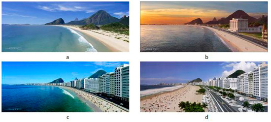
Figure 1.
Copacabana at four time points: (a) 1893 (b) 1927 (c) 1956 (d) 2008. Source: [16].
The sandy site in 1893 (Figure 1a) can still be recognizable in Copacabana in 1927 (Figure 1b), even with the construction of the early buildings, including the imposing presence of the Copacabana Palace Hotel on Atlântica Avenue, on the seaside. In 1956 (Figure 1c), only 29 years later, the intense occupation can already be seen.
In its urban fabric, the neighborhood of Copacabana shows the results of increasing construction activities on the morphology of the original neighborhoods, which were initially designed for low buildings (mostly homes) and relatively large streets (up to 15 m) with trees along them. However, buildings today have templates for more than 12 floors, and there is almost no space between the buildings. All of these changes directly affect the local microclimate. Some of the many aspects that suffer the effects of changes in urban morphology are dynamic ventilation and increased air temperature, resulting in the alteration of the local climate.
The buildings on the waterfront, including their configuration, are very similar to the design currently observed. The major change is the embankment, with the widening of lanes for cars and sidewalks. In 2008, the extent of the sand strip was already significantly higher, as well as the width of the Atlântica Avenue and of the sidewalk (Figure 1d).
3. Material and Method
As the objective of the article is to verify the influence of urban morphology on the microclimate, only the climatic data from 2018 were used in the models of all three time points. Thus, only one criterion was altered in the study: the urban form. To contextualize the analysis, 3D modeling was developed for three historical periods: 1930 (poorly densified), 1950 (medium densification), and 2018 (high densification).
The methodological approach was developed in four successive interconnected phases, which were repeated for the three experiments whenever possible. These stages are (1) the definition of the study area of the survey; (2) the collection of field survey data on urban morphology and climate using the survey of the current maps and historical documents for the development of models; (3) the laboratory work with the computer simulations; and (4) the analysis and comparison of results.
In order to simulate the changes in temperature and ventilation, we used three software packages (ENVI-met [17,18], SOL-AR [19], and RayMan Pro [8]) for the Copacabana neighborhood morphology in three different periods: 1930, 1950, and 2018. ENVI-met [17,18] is a software developed for urban climate simulations, which can represent the impact of architecture and urban planning on the microclimate system, and it was used to perform simulations of the air temperature and ventilation of the studied area. SOL-AR software [19] is a graphics program that provides a sun chart and the compass rose of winds and the average speed frequency of their occurrence according to the specified latitude. Thus, SOL-AR [19] was used for the solar chart and the Rose of the Winds of the chosen latitude. It is an auxiliary tool used to define sun protection, and in the case of the cities whose time data are inserted into its database, it is possible to visualize the annual temperature intervals corresponding to the solar trajectories throughout the year and day. For these locations, it is possible to obtain the wind rose for the frequency of occurrence and average speed for each season of the year in eight orientations (N, NE, L, SE, S, SO, O, NO) [19].
Besides these, the simulations were performed using the software RayMan pro [20], which is a free software program that is continuously updated and developed. It was developed for urban climate studies and has a broader use in applied climatology. The required data to run the simulations in this software are air temperature, humidity, and wind speed. RayMan pro [20] was used to calculate the sky view factor (SVF) and two outdoor comfort indexes—physiological equivalent temperature (PET) and universal thermal climate (UTCI)—in order to determine the effect of morphology changes on thermal sensation.
These three programs are internationally recognized and frequently used in urban experiments; they are also free and easily accessible to any researcher.
The first and immediate procedure was the definition of the study area. This choice followed the criteria of being a densely occupied area but also having open space (green area) and corresponding to a real occupation. There is also the sea to consider since, as mentioned previously, Copacabana is located on a narrow strip of land between the mountains and the sea. There was no intention to work with extreme situations that preclude human presence. The input model was developed from the city plans as a source of historical data to reconstruct, as similar to reality as possible, the urban morphology of 1930 and 1950 and the climatic data of 2018 (as explained in topic 4). In order to complement the identification of the area, fieldwork was carried out to identify the urban morphology and vegetation on a local scale. Then, a survey of the documentation of local weather data for the assembly of the computational models was carried out.
Given the impossibility of having information about the vegetation in the two previous periods, i.e., 1930 and 1950, two simulations for each receptor were generated for 2018: one with vegetation and one without vegetation. Thus, when comparing the results for the three years, it was reason able to expect that their differences were related only to the changes in urban morphology.
Computational Simulations
For carrying out the simulations, three plans of Copacabana were generated: the current neighborhood morphology, the morphology corresponding to 1950, and a sprawling morphology related to 1930. Old photographs were helpful for finding the heights of some buildings, as well as for identifying the plans that were supplied by the IPP (Pereira Passos Institute) [21] from Rio de Janeiro city. To deal with this issue, a deconstruction process was conducted to establish the heights and positioning of buildings. It is necessary to clarify that some approximations were needed since it was not possible to acquire continuous data on the height of buildings; this mostly applied to building height and positioning data for the year 1930.
ENVI-met [17,18] is a three-dimensional model that was developed to simulate climatic variables in urban environments. The simulation process combines interactions between climatic variables and urban morphology and integrates four main systems—soil, vegetation, atmosphere, and construction—whose information is inserted as input files. The basic equations of the physical model are related to the mean air flow; temperature and humidity of the air; soil temperature; turbulence processes and thermal changes; and radioactive flux.
The atmospheric model calculates air movement, three-dimensional turbulence, air temperature, and relative humidity while taking into account obstacles such as buildings and vegetation. The surface model calculates the emitted long-wave length waves and the reflected shortwave radiation from different surfaces using the surface temperature values defined (initially) and calculated in the simulation process. For vegetation, there is a specific model that allows the detailing of the type of vegetation, which is characterized not only by its height but also by the normalized leaf area density (DAL) and normalized root area density (RAD). Thus, vegetation can be selected to more appropriately reflect the local reality. The airflow and tree shape fields enable calculations of the rate of evaporation and turbulence around the vegetation. The soil model calculates the thermal and hydrodynamic processes that occur in the soil and accounts for the combination of natural and artificial surfaces, as well as the presence of water bodies and their environment.
ENVI-met [17,18] also allows for the punctual reading of results through the insertion of receptors. For this, an output file (named for each receiver) is generated, with point values that refer to that position. Thus, for a specific altitude and position, it is possible to observe the temperature and humidity of the air of the space specified by the user. The input file with climatic data requires air temperature and absolute humidity measured at a 2500-m altitude and wind speed and direction relative to the humidity measured at 2 m, as well as the coefficient of roughness of the terrain. Other data, such as the temperature and humidity of the soil, transmissivity of the surfaces (albedo), and gases and particles in the atmosphere (CO2 concentration), can be input in addition to the required data.
Schematic drawings and official maps were used in the definition and presentation of the study area, as well as in the determination of the parameters of analysis. Figure 2 shows a graphical representation of the area with soil coverage specifications, including the vegetation, and buildings related to (a; a1) Sprawl Morphology (urban form data: 1930), (b; b1) Medium Morphology (urban form data: 1950), and (c; c1) Density Morphology (urban form data: 2018). The images labeled a1, b1, and c1 of Figure 2 are volumetric 3D displays (illustrative).
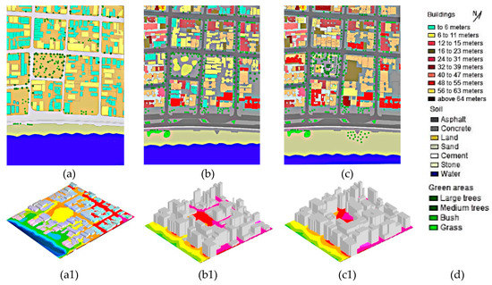
Figure 2.
Description of the input file area for ENVI-met: (a; a1) Sprawl Morphology (urban form data: 1930); (b; b1) Medium Morphology (urban form data: 1950); (c; c1) Density Morphology (urban form data: 2018).The legends indicate the building heights and soil coverage (d).
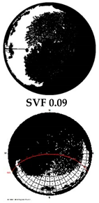
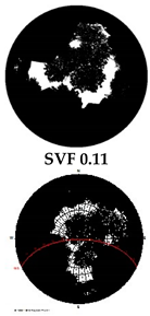
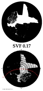
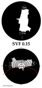
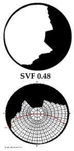
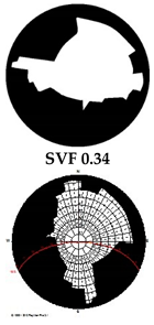
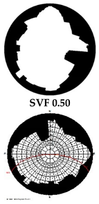
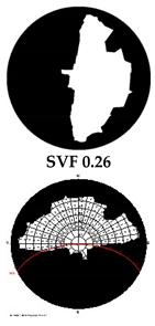
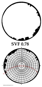
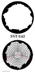
In the input model, four specific points were determined for the placement of the Receptors and from which the data were measured in a timely manner. Determining the placement of these receptors involved considerations of the geographic location and its surroundings; i.e., the receptors were located in regions that are characterized by different urban morphologies and distances from the sea. From these points (Figure 2c), images were taken using fisheye lenses to calculate the sky view factor (SVF) and the solar path using the RayMan pro [20]. The fisheye images and the SVF values can be used to identify changes in urban morphology in the years 1930, 1950, and 2018, and the images show the gradual confinement of the region. Fisheye images of the morphologies for the 1950s and 1930s were made from three-dimensional models of the areas. In this way, it was possible to observe the direct effect of the morphology on the sky vision factor, which is one of the characteristics that can directly influence the microclimate.
The calculation of the SVF using RayMan from the fisheye lens images was developed to determine the location of the receivers. Thus, the process allows for exploring the different configurations found in the region, such as the sea border, proximity to green area, and urban canyon. The values presented in Table 1 were calculated from 3D geometry, and the values observed at the observer points coincide with those calculated for these points.

Table 1.
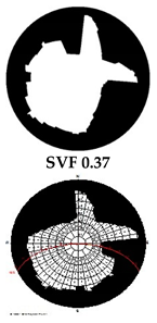
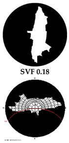
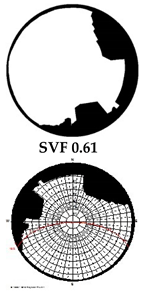
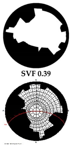
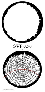
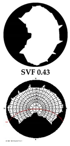
Images of the sky taken with a fisheye lens, black and white masks, sky view factor (SVF), and the solar path.
Table 1 shows the images of the sky taken with a fisheye lens, followed by the images generated for calculating the sky view factor (SVF) and the solar path [20]. Each of the receptors is identified through its latitude and longitude indicated in Table 1, header row. As stated earlier, we generated two images of the SVF for the year 2018, one with and one without vegetation, to compare the results with those of the previous years (1930 and 1950) and observe changes in the urban morphology.
From Table 1, it is already possible to observe that, for example, at Receptor 4, the SVF presented a decrease of more than 50% over the years. This reduction in the SVF represents an extensive increase in confinement for that area and its surroundings. In the case of Receptor 1, its position is an exception since it is facing the sea with views of Copacabana Beach. From the trajectory of the solar path measured in the summer, it is possible to observe the blocking of the morning sun for the Receptors 2 and 4, and for Receptor 4, there is almost complete sun blocking, except for periods of more intense sunlight (12 p.m.).
The input with the information necessary for the computer simulations was based on actual data. For the initial condition, the air temperature value was calculated from the average in January 2018 obtained from National Institute of Meteorology (INMET) [22]. The aim was to use data from the summer and not the whole year because, in a city with a tropical climate, summer is the season with the highest number of days of thermal discomfort. The choice was made not to use data from a particular day to avoid the risk of selecting an atypical summer day as the reference.
Atmospheric data applicable to the boundary conditions were read from the archives of the Galeão Airport weather station [23]. Information regarding the geometry of the domain was obtained from a data warehouse, IPP [21], from Rio de Janeiro city. All simulations were done with the same meteorological data, i.e., the average of January of 2018, in order to clarify that the changes observed were attributable to changes in urban morphology and loss of vegetation cover.
ENVI-met includes a three-dimensional modeling process, in which the smallest unit is a cube with the dimensions dx, dy, and dz, called a grid cell, which, when side by side, will increase the volume in three dimensions from the simplified representation of the region. To begin to represent the area to be modeled in the program, it is necessary to establish the grid to be used, that is, to determine how many of these cubes amount to the volume of the area extension (which must be square or rectangular) as well as the height and size of each one. The size of the cells influences the accuracy of the data obtained since, to model the area, it is necessary to designate the part of the urban morphology to which each grid cell belongs. The simulated area was 390 m × 570 m and defined in a grid of 3 × 3 to generate the ENVI-met input file.
The largest building is 60 m high, and it is necessary to apply the telescopic grid feature beyond this height so that the program has the space to perform its calculations. Next, it is necessary to define the parameters of the urban forms to be represented. For modeling the trees, the chosen types “MO” (tree with a 20-m height, medium density, and no crown defined) because it is the one that best fits the vegetation found in the neighborhood. For modeling buildings, the software requests only its height in meters. In order to estimate the heights, the floor counts of each of the buildings within the area were counted (in addition to the ground floor), with a 3-m height per floor assumed. For example, a building with nine floors and the ground floor was estimated to be 30 m high.
Once the model area is established, the program requires the configuration of the boundary conditions so that it can carry out the modeling. The initial time of the simulation was 9:00 p.m. on January 23, 2018 (this date was set only for the program reference, but the input data values refer to January 2018 averages). We simulated 48 h for each model with recordings of 60 in 60 min. At this stage, the ENVI-met software did not yet account for heat generation of anthropic origin.
The climatic input data were as follows: the wind speed at 10 m is 3.0 m/s; the wind direction is 135 SE; the roughness length z0 at the reference point is 0.1; the initial temperature atmosphere [K] is 309.85 K (36.7 °C); the specific humidity at 2500 m [g water/kg air] is 10.3 g water/kg air and the relative humidity at 2 m is 75.01%.
The direction and velocity of the prevailing winds for the Rio de Janeiro city were obtained using the software SOL-AR [7]. In the summer, the highest frequency of the winds was found to be southeast, with maximum velocities around 3 m/s. The predominance of the southeast winds occurs in all seasons. Computer simulations were performed using the software ENVI-met [17,18], which was developed for climate simulations in urban areas. Leonardo software 3.75 [17,18] was used for visualization of the results.
4. Results and Discussions
The obtained results from the simulations with ENVI-met were compared with measured data provided by the Municipal Environment SMAC [24]. The measured and predicted hourly (from 9:30 a.m. and 12:30 p.m.) air temperatures (Ta) for the point at Receptor 1 are compared in Figure 3, which shows the similarity between the results.
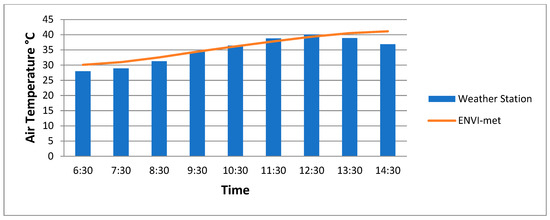
Figure 3.
Relationship between predicted and measured Ta for Receptor 1: 9:30 a.m. to 12:30 p.m.
Weather station data and simulated (ENVI-met) air values are close, with a relatively short time interval. There is a difference between the measured and simulated values for the time at which the air temperature values begin to fall. For the measured data, this moment occurs at 12:00 p.m., whereas for the simulated values, this point occurs at 2:30 p.m.; also, the temperature decreases at a much slower rate than that observed in the measured values.
In this work, the simulation results are presented for two specific hours that are representative of the region: 10 a.m. and 8 p.m. The former is a time of intense solar radiation in Rio de Janeiro city, and the latter is two hours after sunset. It is interesting to observe the effects on the environment of exposure to intense heat during the day. Figure 4 shows the temperature results for 10 a.m. From this figure, it is notable that in the configuration for 1930, much of the region does not reach 35 °C. From the density and changing urban morphology, the observed temperature on the block experienced an average increase of almost 3 K. Even for a non-quantitative analysis, these results are interesting because the simulations were made, as previously mentioned, with 2018 climate data, thus leaving the variations between models due to changes in the urban morphology only.
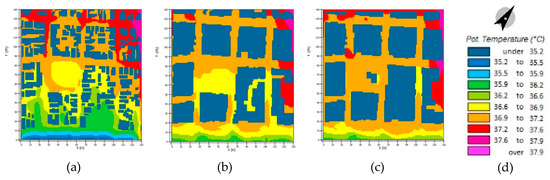
Figure 4.
Air temperature (Ta) results for January 2018 (average), 10 a.m.: (a) Sprawl Morphology (urban form data: 1930); (b) Medium Morphology (urban form data: 1950); (c) Density Morphology (urban form data: 2018); and (d) Color scale and north.
Figure 5 shows the temperature results for 8 p.m. From the images, it is possible to see, as observed in practice, which configuration has the highest capacity to store heat from urban coatings. A high capacity to store heat is associated with ventilation barriers that hinder heat dissipation. Then, the decrease in the temperature at night is slightly felt because of the intense density and ground cover.
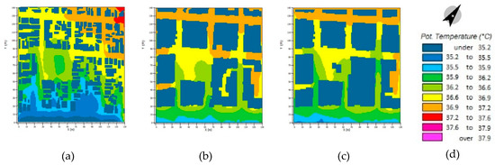
Figure 5.
Air temperature (Ta) results for January 2018 (average), 8 p.m.: (a) Sprawl Morphology (urban form data: 1930); (b) Medium Morphology (urban form data: 1950); (c) Density Morphology (urban form data: 2018); and (d) Color scale.
Figure 6 and Figure 7 present the results for air humidity (%) and ventilation (m/s), respectively, for 8 p.m.
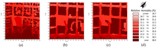
Figure 6.
Humidity (Hu) results for January 2018 (average), 8 p.m.: (a) Sprawl Morphology (urban form data: 1930); (b) Medium Morphology (urban form data: 1950); (c) Density Morphology (urban form data: 2018); and (d) Color scale.
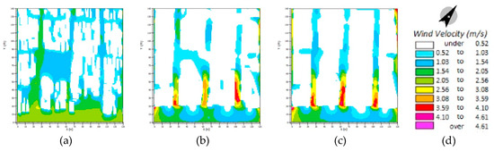
Figure 7.
Ventilation (m/s) results for January 2018 (average), 8 p.m.: (a) Sprawl Morphology (urban form data: 1930); (b) Medium Morphology (urban form data: 1950); (c) Density Morphology (urban form data: 2018); and (d) Color scale.
According to the images in Figure 5, as explained, the decrease in night air temperature is weak in intense density configurations. In parallel, the highest values of air humidity (Figure 6) are present in the scattered configuration, that is, the one corresponding to the urban morphology of 1930. The distribution of air ventilation (Figure 7) within the blocks is the worst for the 1950 and 2018 configurations because of the densification process adopted in Copacabana. It should be noted that besides verticalization in the neighborhood, there was a marked reduction in the distance between buildings, so an urban mesh with little permeability has formed.
The highest values of air ventilation intensity can be found at wind entry corridors. However, internally, the intensity is significantly reduced. In a city such as Rio de Janeiro, air ventilation affects directly thermal sensation and, therefore, the use of spaces.
The SVF values for the three configurations are presented in Figure 8. From the results, there is a reduction in the SVF from the verticalization process, as well as a reduction in the spacing between buildings.
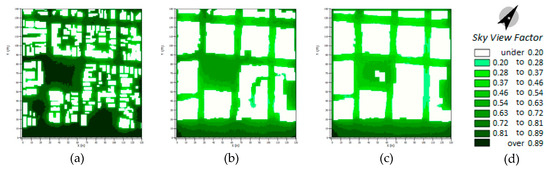
Figure 8.
Sky view factor results for (a) Sprawl Morphology (urban form data: 1930); (b) Medium Morphology (urban form data: 1950); (c) Density Morphology (urban form data: 2018); and (d) Color scale.
As shown in the images in Figure 8, the design of the blocks has not changed, but the replacement of the original buildings of 1 and 2 decks has resulted in these reduced SVF values. Even the Serzedelo Correa square, the most open area in the interior of the neighborhood, given the construction of its surroundings, presents a reduction in the SVF by almost half of its value in 1930, thus implying a reduction in insolation.
To determine the effect of the morphology of the studied region on thermal sensation, the physiological equivalent temperature index (PET; Figure 9) was calculated; the PET is an index based on the Munich energy-balance model for individuals (MEMI), developed by Höppe [25] and very frequently used in outdoor studies. The PET was calculated using the software RayMan pro [20], with inputs comprising the values calculated at each receiver for air temperature (Ta), relative humidity (RH), wind velocity (v), and mean radiant temperature (TMRT). Data for the average man were used with the default tool for the calculation: age of 35 years old, height of 1.75 m and weight of 75 kg, and metabolic rate of 80 W (light activity).
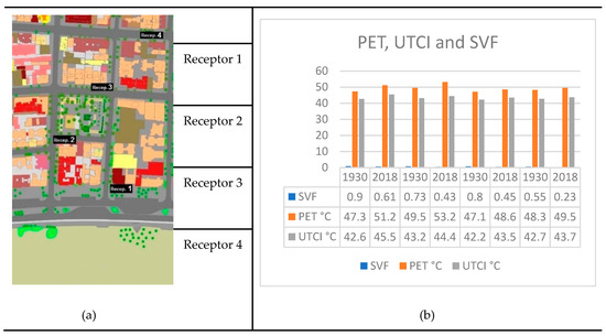
Figure 9.
Location of Receptor (a) and Results for Physiological Equivalent Temperature (PET), Universal Thermal Climate Index (UTCI), and Sky View Factor (SVF) (b).
Another index adopted here is the Universal Thermal Climate Index (UTCI) [26] (Figure 9). It is similar to other indices used to evaluate outdoor temperature conditions, such as PET, as it adopts the concept of an equivalent temperature. Calculating the UTCI requires Ta, TMRT, RH, and v. The premise of this index is the satisfaction of the following requirements: “thermo physiologically significant in the whole range of heat exchange; valid in all climates, seasons and scales; useful for key applications in human biometeorology (e.g., daily forecasts, warnings, regional and global bioclimatic mapping, epidemiological studies, and climate impact research); independent of person’s characteristics (age, gender, specific activities and clothing etc.)” (http://www.utci.org/index.php). Its calculation can be done online at the UTCI website (http://www.utci.org/utcineu/utcineu.php). Both PET and UTCI were calculated from the output data of the simulation times with ENVI-met.
From the values presented in Figure 9, the following observations can be made:
- -
- For all four receptors, the observed increase in temperature related to the thermal sensation corresponds with the increased densification of the region;
- -
- The SVF shows a reduction, even in the edge area (Receiver 1), due to the increase in the height of the buildings;
- -
- In the scattered configuration, which is consistent with the 1930 model, as well as in the dense configuration, the lowest values for both the PET and UTCI are observed at Receiver 3, that is, near Serzedelo Correa Square and the corridor of Hilário de Gouveia street, and these areas promote the direct entry of wind in the region, as can be seen in Figure 9;
- -
- From the values of PET and UTC in the graph in Figure 9, it is noticeable that the values for all the receivers increase with the densification and verticalization of the model.
According to the “heat stress” categories for PET defined by Matzarakis and Mayer [27] and calibrated by Krüger et al. [28], for the city of Rio de Janeiro, in terms of thermal sensitivity, all of the points studied for the two configurations fall into the “hot” and “very hot” categories in the summer in the city of Rio de Janeiro. From analyzing the thermal comfort/stress categories, one can group the obtained results into “heat stress” and “extreme heat stress” (Table 2).
Table 2.
Comfort and heat categories for PET and UTCI. Adapt by [29,30].
From the results presented in Figure 9, it can be seen that the values found for all cases studied show that the thermal sensation blocks are in the range of “extreme heat stress”. It is also observed that reducing the SVF corresponds with an increase in the indexes; data from the Receptor 1 position, which is situated on the beach of Copacabana, indicates that the PET index (Figure 9) increased by nearly 4 °C. The increase observed at Receptor 1 is likely the result of the effect of the large increase in the stretch of sand and the consequent detachment of the sea. Measurements from Receptor 2 show that the highest temperature values occurred in 2018. This is because of blocked ventilation (southeast direction), as the right-side block forms an almost compact block, and there is no road that wind can access coming from the southeast, as in the cases of Receptors 3 and 4. Receptor 4 shows the lowest temperatures. Located in a canyon position, this location receives intense southeast ventilation if the direction of the wind is considered the primary factor, although the blockade of partial solar radiation is likely to contribute to these lower values.
As shown by Krüger et al. [31], although the measured and calculated results include the “heat stress” and “extreme heat stress” categories for both indexes, the effect on thermal sensation may not be clear because, according to the perceptions of individuals in regions of the city, acclimatization to the city’s climate contributes to the experienced effects.
5. Conclusions
A survey was conducted related to urban morphology in Copacabana, Rio de Janeiro, to study the relationship between the microclimate and urban form, which was exemplified by the morphology of the neighborhood in 1930, 1950, and 2018. This location has been under a constant process of change over the years, and it is possible to observe the consequences in terms of temperature and thermal sensation. Some assumptions were necessary; for example, assumptions were made in the construction of 3D models and the calculation of the SVF for the 1930s and 1950s because there were insufficient images for the reconstruction of the real scene. However, simulations of the three scenarios were performed for the same conditions since the objective of the research is to assess the microclimate changes resulting from the morphological changes.
In Figure 9, which presents the values of the sky view factor, PET, and UTCI indexes, it is possible to observe an increase in temperature associated with a reduction in the value of the SVF at the sites of the four analyzed receptors. This is an indicator that an increase in local temperature is an effect of urban morphology densification.
Moreover, a decrease of approximately 50% of the sky view factor between the years 1930 and 2018 is observed at virtually all receiver locations. This is in addition to the formation of urban canyons, which act as ventilation channels and reduce the permeability of the blocks, translating to the thermal discomfort experienced inside the buildings. This can also be explained by the fact that in addition to the growth of vertical buildings, the routes have remained the same size and almost all of the grounds have very high occupancy rates.
The analysis of temperature values reveals that temperature differences are related to changes in urban morphology. This behavior is observed even in the case of the temperature increase in the sea side region, where an important extension of the stretch of sand and asphalt road actually occurred away from the sea.
In the ENVI-met results, even in open areas such as in Serzedelo Correa square, there was an increase in temperature. This is due to the densification and increase of reflective materials in buildings and ground cover.
In addition, changes in ventilation dynamics and relative humidity measurements are observed. The first scenario (referring to the morphology of 1930) presents better ventilation permeability and similar wind velocities throughout the territory. However, the urban form of 2018 shows an excessive increase in wind speed at the beginning of the routes perpendicular to the beach. This is due to the formation of canyons by the buildings. In addition, the standardization of volumetry impairs the permeability of ventilation.
All the results corroborated for the assertion of the hypothesis that the morphology interferes directly in the local microclimate. In the case of tropical cities, the increase in temperature and the change in the dynamics of the winds can cause islands of heat. In addition, it can contribute to the increase of the energy consumption from the greater use of conditioned air to soften the internal temperatures.
From the discussions presented in the article, it is argued that it is essential to consider the microclimatic conditions of the region to better plan urban occupation. It is also argued that further studies are needed in cities located in tropical regions before allowing their densification.
Author Contributions
Conceptualization, G.S.B., P.R.C.D. and O.D.C.; methodology, G.S.B. and P.R.C.D.; software, G.S.B. and P.R.C.D.; validation, G.S.B., P.R.C.D. and O.D.C.; formal analysis, G.S.B., P.R.C.D. and O.D.C.; investigation, G.S.B., P.R.C.D.; resources, G.S.B., P.R.C.D.; data curation, P.R.C.D.; writing—original draft preparation, G.S.B., P.R.C.D.; writing—review and editing, G.S.B., P.R.C.D. and O.D.C.; visualization, G.S.B.; supervision, O.D.C.; project administration, O.D.C.; funding acquisition, O.D.C. and P.R.C.D.
Funding
This research was funded by Brazilian funding agencies: Conselho Nacional de Desenvolvimento Científico e Tecnológico–CNPq, Coordenação de Aperfeiçoamento de Pessoal de Nível Superior—CAPES and FAPERJ (Fundação Carlos Chagas Filho de Amparo à Pesquisa do Estado do Rio de Janeiro).
Conflicts of Interest
The authors declare no conflict of interest.
References
- Rogers, R. Cidades Para um Pequeno Planeta; Editora Gustavo Gilli: Barcelona, Spain, 2001. [Google Scholar]
- Barbosa, G.S.; Drach, P.R.C.; Corbella, O.D. A Comparative Study of Sprawling and Compact Areas in Hot and Cold Regions. In Proceedings of the World Renewable Energy Congress WREC XI, Abu Dhabi, United Arab Emirates, 25 September 2010; Volume 1, pp. 1–6. [Google Scholar]
- Barbosa, G.S.; Drach, P.R.C.; Corbella, O.D. Um Estudo Comparativo de Regiões Espraiadas e Compactas: Caminho para o Desenvolvimento de Cidades Sustentáveis. In Proceedings of the Congresso Internacional Sustentabilidade e Habitação de Interesse Social—CHIS, Porto Alegre, Brazil, 18 June 2010; Volume 1, pp. 1–10. [Google Scholar]
- Drach, P.R.C.; Corbella, O.D. Estudo das Alterações na Dinâmica da Ventilação e da Temperatura na Região Central do Rio de Janeiro: Mudanças na Ocupação do Solo Urbano. In Proceedings of the 4° Congresso Luso-Brasileiro para o Planejamento Urbano, Regional, Integrado e Sustentável—PLURIS, Faro, Portugal, 29 October 2010; Volume 1, pp. 1–12. [Google Scholar]
- Girardet, H. Creating Sustainable Cities; Green Books: Bristol, UK, 2007. [Google Scholar]
- Corbella, O.D.; Yannas, S. Em Busca de Arquitetura sustentável para os Trópicos; Editora Revan: Rio de Janeiro, Brazil, 2003. [Google Scholar]
- Romero, M.A.B. Arquitetura Bioclimática do Espaço Público; Editora Universidade de Brasília: Brasília, Brasil, 2001. [Google Scholar]
- Romero, M.A.B. Correlação entre o Microclima Urbano e a Configuração do Espaço Residencial de Brasília. In Proceedings of the ENCAC—Encontro Nacional de Conforto no Ambiente Construído, Natal, Brasil, 16–18 September 2009. [Google Scholar]
- Nobre, E.A.C. Desenvolvimento Urbano e Sustentabilidade: Uma Reflexão sobre a Grande São Paulo no Começo do Século XXI. In Proceedings of the Núcleo de Pesquisa em Tecnologia da Arquitetura e Urbanismo—NUTAU, São Paulo, Brazil, 18–21 July 2004. [Google Scholar]
- Lombardo, M.A. Ilha de CalornasMetrópoles: O Exemplo de São Paulo; Editora HUCITEC: São Paulo, Brazil, 1985. [Google Scholar]
- De Moura Rodrigues, F. Desenho Urbano: Cabeça Campo e Prancheta; Projeto: São Paulo, Brazil, 1986. [Google Scholar]
- IBGE—Instituto Brasileiro de Geografia e Estatística. “Censo Demográfico 2010 e Base de informações por setor censitário do Censo Demográfico 2010”. IBGE: Rio de Janeiro, Brazil, 2010. Available online: http://www.ibge.gov.br/home/ (accessed on 25 March 2018).
- Von der Weid, E. O Bonde Como Elemento de Expansão Urbana no Rio de Janeiro; Setor de História da Fundação Casa de Rui Barbosa: Rio de Janeiro, Brazil, 2004. [Google Scholar]
- Cardoso, E.D. História dos bairros do Rio de Janeiro–Copacabana; Editora Index: Rio de Janeiro, Brazil, 1986. [Google Scholar]
- Vaz, L.F. Modernidade e Moradia: Habitação coletiva no Rio de Janeiro, Séculos XIX-XX; 7 Editora Letras: Rio de Janeiro, Brazil, 2002. [Google Scholar]
- Pereira, C.G.N. Copacabana–Mini Pranchas; Instituto Pereira Passos/IPP: Rio de Janeiro, Brazil, 2008. [Google Scholar]
- Bruse, M. “ENVI-met. Version 3.1 BETA III–2009” and “LEONARDO 3.75–2009”. Software and on-line Manual. Available online: http://www.envi-met.com (accessed on 21 June 2018).
- Bruse, M. “LEONARDO 3.75–2009. On-line Manual”. Available online: http://www.envi-met.com (accessed on 21 June 2018).
- SOL-AR Software. Laboratório de Eficiência Energética em Edificações––LabEEE, Departamento de Engenharia Civil (ECV)—Universidade de Santa Catarina (UFSC). 2013. Available online: http://www.labeee.ufsc.br/downloads/softwares/analysis-sol-ar (accessed on 21 June 2018).
- Matzarakis, A.; Rutz, F.; Mayer, H. Modelling radiation fluxes in simple and complex environments: Basics of the RayMan model. Int. J. Biometeorol. 2010, 54, 131–139. [Google Scholar] [CrossRef] [PubMed]
- IPP—Instituto Municipal de Urbanismo Pereira Passos. “Armazém de Dados”. Prefeitura do Rio de Janeiro, 2013. Available online: http://www.armazemdedados.rio.rj.gov.br/ (accessed on 25 March 2018).
- INMET—Instituto Nacional de Meteorologia. Relatórios de Dados Meteorológicos. Consulta Dados da Estação Convencional: Rio de Janeiro, Brazil, 2013. Available online: http://www.inmet.gov.br/portal/ (accessed on 25 March 2018).
- University of Wyoming. Department of Atmospheric Science. Upper Air Maps. Galeão Weather Station (83746 Galeão—SBGL), 2013. Available online: http://weather.uwyo.edu/upperair/sounding.html (accessed on 21 June 2018).
- CPTEC—Centro de Previsão de Tempo e Estudos Climáticos/INPE—Instituto Nacional de Pesquisas Espaciais. Ministério da Ciência e Tecnologia, Cachoeira Paulista, SP. 2013. Available online: http://www.cptec.inpe.br/ (accessed on 25 March 2013).
- Höppe, P. The Physiological Equivalent Temperature: A index for the biometeorological assessment of the thermal environment. Int. J. Biometeorol. 1999, 43, 71–75. [Google Scholar] [CrossRef] [PubMed]
- Bröde, P.; Krüger, E.L.; Rossi, F.A.; Fiala, D. Predicting urban outdoor thermal comfort by the Universal Thermal Climate Index UTCI—A case study in Southern Brazil. Int. J. Biometeorol. 2012, 5, 471–480. [Google Scholar] [CrossRef] [PubMed]
- Matzarakis, A.; Mayer, H. Another kind of environmental stress: Thermal stress. WHO Newsl. 1996, 18, 7–10. [Google Scholar]
- Krüger, E.L.; Rossi, F.A.; Drach, P.R.C. Calibration of the physiological equivalent temperature index for three different climatic regions. Int. J. Biometeorol. 2017, 61, 1323–1336. [Google Scholar] [CrossRef] [PubMed]
- Matzarakis, A.; Mayer, H. Heat stress in Greece. Int. J. Biometeorol. 1997, 41, 34–39. [Google Scholar] [CrossRef] [PubMed]
- Bröde, P.; Fiala, D.; Błażejczyk, K.; Holmér, I.; Jendritzky, G.; Kampmann, B.; Tinz, B.; Havenith, G. Deriving the operational procedure for the universal thermal climate index (UTCI). Int. J. Biometeorol. 2012, 56, 481–494. [Google Scholar] [CrossRef] [PubMed]
- Krüger, E.L.; Drach, P.R.C.; Bröde, P. Outdoor comfort study in Rio de Janeiro: Site-related context effects on reported thermal sensation. Int. J. Biometeorol. 2017, 61, 463–475. [Google Scholar] [CrossRef] [PubMed]


© 2019 by the authors. Licensee MDPI, Basel, Switzerland. This article is an open access article distributed under the terms and conditions of the Creative Commons Attribution (CC BY) license (http://creativecommons.org/licenses/by/4.0/).