Basin-Scale Vegetation Sensitivity to Relative Humidity Variability Across Türkiye Under CMIP6 SSP Pathways

Abstract

Relative humidity (RH) provides complementary information on atmospheric moisture conditions that is not captured by precipitation alone. This study characterizes basin-scale RH-associated vegetation sensitivity across Türkiye’s 25 hydrographic basins using MODIS MOD13A1 NDVI observations for 2000–2024 and processed CMIP6-derived RH products for SSP1-2.6, SSP2-4.5, SSP3-7.0 and SSP5-8.5 at the 2040, 2060, 2080 and 2100 single-year horizons. MODIS and climate-model products are summarized independently at basin scale, avoiding pixel-level fusion across different native resolutions. The archived 25-by-4 pathway sensitivity matrix is evaluated using cross-pathway dispersion, a robust median-magnitude check, hierarchical clustering with silhouette diagnostics, and explicit percentile-based hotspot criteria. Mean absolute sensitivity is 0.0244, 0.0236, 0.0368, and 0.0386 under SSP1-2.6, SSP2-4.5, SSP3-7.0, and SSP5-8.5, respectively. Antalya, Küçük Menderes, Konya Closed, Ceyhan, and Aras satisfy the magnitude and persistence criteria, and all five also exceed the upper-quartile threshold for median absolute sensitivity. Silhouette diagnostics do not support a unique three-cluster solution, favoring explicit threshold-based response classes. The results are interpreted as comparative basin screening rather than causal attribution or validated vegetation forecasting. Because the retained processed products do not preserve model/member provenance or the horizon-level intermediate values used to generate the pathway index, model-specific and predictive interpretations are deliberately avoided.

1. Introduction

Vegetation dynamics emerge from interacting climatic, hydrological, and land-management controls. Temperature, precipitation, radiation, soil-water availability, and atmospheric demand can change simultaneously, and their effects need not be spatially uniform. In Mediterranean and semi-arid transition environments, increases in atmospheric dryness may constrain vegetation activity even where annual precipitation does not show a simple monotonic decline [1,2,3,4,5].

The normalized difference vegetation index (NDVI) remains widely used for regional monitoring of canopy greenness and vegetation–climate interactions [6,7,8,9]. Its climatic controls vary with biome, season, drought time scale, land cover, and human intervention [10,11,12,13]. Atmospheric moisture is relevant because humidity is linked to stomatal regulation, evaporative demand, and plant water loss [14,15,16,17,18]. Relative humidity (RH), however, is not interchangeable with vapor pressure deficit (VPD), nor can an RH–NDVI relationship by itself establish a causal vegetation response. The present analysis therefore treats RH as a screening variable for atmospheric-moisture exposure rather than as a complete ecohydrological driver.

A clear separation between observation and climate-model information is required for scenario analysis. MODIS NDVI is used here to characterize observed vegetation conditions, whereas the RH layers represent processed CMIP6-derived climate information. The climate-model reference RH term and the future SSP RH layers are therefore kept distinct from the satellite vegetation baseline. No future vegetation map is treated as an observation or as an independently validated forecast in the revised analysis.

The CMIP6 ScenarioMIP framework provides coordinated simulations under alternative socioeconomic and radiative-forcing pathways [19,20,21,22,23]. These simulations have been used extensively to investigate drought and hydroclimatic risk [24,25,26,27]. Türkiye is a useful test region because its 25 hydrographic basins include humid maritime catchments, semi-arid interiors, high-elevation eastern basins, and heavily managed agricultural systems. A national average can therefore conceal markedly different responses to atmospheric moisture loss.

The objective is to identify where RH-associated vegetation sensitivity is comparatively strong and persistent across SSP pathways, without attributing vegetation change to RH alone. Specifically, the study (i) compares basin-scale RH patterns across four SSPs and four future horizons; (ii) evaluates an archived scenario-specific NDVI–RH sensitivity matrix; (iii) quantifies cross-pathway dispersion and robust central magnitude; (iv) tests hierarchical-clustering stability using silhouette diagnostics; and (v) applies explicit percentile-based hotspot thresholds. The analysis is framed as comparative basin screening and does not treat the sensitivity index as a causal effect or a calibrated predictive model.

2. Materials and Methods

2.1. Study Area

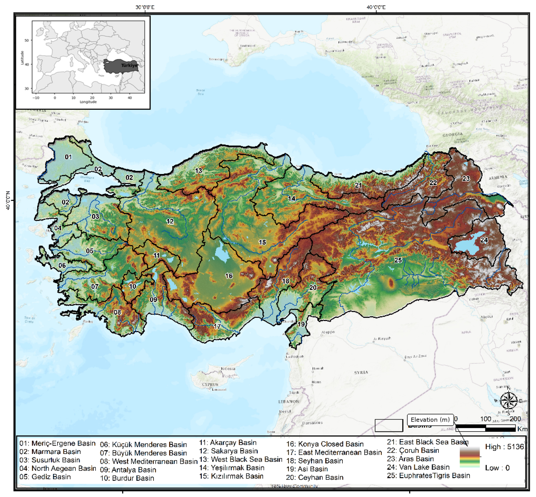
The analysis covers Türkiye’s 25 hydrographic basins (Figure 1). The basin system spans humid Black Sea catchments, Mediterranean coastal basins, semi-arid interior basins, high-elevation eastern basins, and closed basins affected by intensive water management. This environmental contrast permits the same atmospheric-moisture indicator to be evaluated across substantially different hydroclimatic settings.

2.2. Data Streams, Baselines and Scenario Design

Three data roles are distinguished throughout the analysis: observed vegetation, the climate-model reference RH term, and future SSP climate states. MODIS MOD13A1 NDVI for 2000–2024 is the observational vegetation record. MOD13A1 provides 16-day vegetation-index observations at 500 m spatial resolution [6,9,28,29]. Google Earth Engine was used for collection access, quality screening, temporal compositing, and basin extraction [30,31,32]. The quality-controlled long-term basin mean defines $NDV{I}_{i,0}$, the observed greenness baseline for basin i.

The climate component consists of processed CMIP6-derived RH products for SSP1-2.6, SSP2-4.5, SSP3-7.0 and SSP5-8.5 [19,22,23]. The available future layers correspond to 2040, 2060, 2080, and 2100 and represent single-year horizons rather than moving windows or 20-year climatologies. The term $R{H}_{i,0}$ denotes the basin-level reference RH value associated with the processed climate product. It is a climate-model reference quantity and is not treated as an observed-humidity measurement.

Table 1. Data sources, temporal/spatial support and analytical roles. The climate-model reference RH term is distinct from the observed MODIS vegetation baseline.

Stream	Temporal Support	Spatial/Retained Support	Role in This Study
MODIS MOD13A1 NDVI	2000–2024; native 16-day	500 m; summarized by basin	Observed vegetation baseline, $NDV{I}_{i,0}$
Processed CMIP6 reference RH	Reference layer associated with the processed product	Climate-model grid; summarized by basin	Climate-model reference term, $R{H}_{i,0}$; not observed RH
Processed CMIP6 SSP RH	2040, 2060, 2080, 2100 single-year horizons	Climate-model grid; summarized by basin	Future scenario-conditioned RH states
Sensitivity matrix	One value per basin and SSP	25 basins × 4 SSPs	Derived input to dispersion, clustering and hotspot analyses

summarizes the distinct data roles and supports.

The processed RH products available for this study do not retain the contributing GCM names, realization/member identifiers, native grid metadata, or the exact CMIP6 reference-period description. These attributes cannot be reconstructed reliably from the figure-ready raster exports. The results are therefore reported at the level of the processed SSP products and are not attributed to a specific GCM, realization, or multi-model ensemble configuration. The consequences of this provenance limitation are addressed in Section 4.

2.3. Spatial Harmonization and Temporal Aggregation

MODIS NDVI and CMIP6-derived RH were not fused at native pixel resolution. Each source was summarized independently within the same hydrographic-basin boundaries and linked by basin identifier. This basin-level harmonization avoids implying that the 500 m MODIS raster was interpolated to an undocumented climate-model grid, or that the climate-model RH field was downscaled to 500 m. The available processing record confirms basin masking and basin-scale aggregation but does not preserve sufficient low-level metadata to verify the treatment of partial edge cells or any model-specific resampling step. No unverified area-weighting, bias-correction, or downscaling algorithm is therefore attributed to the original workflow. Basin aggregation addresses the mismatch in spatial support; it does not correct climate-model bias.

The MODIS vegetation baseline is a 2000–2024 long-term summary derived from quality-controlled 16-day observations. The RH scenario products are single-year horizon layers. The resulting sensitivity matrix is therefore a long-term basin-scale screening product and cannot resolve growing-season phenology, crop-calendar effects, or delayed vegetation responses. These temporal limitations and the analyses required to address them are discussed in Section 4.

2.4. Scenario-Specific Sensitivity Matrix

The analytical dataset contains a 25-by-4 matrix of scenario-specific finite-change sensitivity indices. For basin i and SSP pathway s, the index is represented as

$$\mathrm{\Delta }NDV{I}_{i,s}=NDV{I}_{i,s}-NDV{I}_{i,0},\mathrm{\Delta }R{H}_{i,s}=R{H}_{i,s}-R{H}_{i,0},$$

(1)

$${\beta }_{i,s}={\displaystyle \frac{\mathrm{\Delta }NDV{I}_{i,s}}{\mathrm{\Delta }R{H}_{i,s}}},\mathrm{\Delta }R{H}_{i,s}\ne 0.$$

(2)

The SSP subscript identifies the pathway-specific finite-change index; ${\beta }_{i,s}$ is not treated as an ordinary historical OLS regression slope. Its sign records the direction of the paired RH–NDVI change, whereas $|{\beta }_{i,s}|$ records its magnitude. The retained research materials contain the final 25-by-4 pathway matrix but not the horizon-level $\mathrm{\Delta }NDVI$ and $\mathrm{\Delta }RH$ arrays or the exact operator that reduced the four horizon-specific quantities to one pathway-level value. Consequently, the matrix is treated as an archived derived input rather than as a coefficient that can be re-estimated from the currently retained intermediates. This boundary is important: the downstream descriptive, clustering, and hotspot analyses are reproducible from Supplementary Table S1, whereas the upstream pathway-index generation requires the original intermediate data and is not reconstructed by assumption. Downstream analyses are therefore conducted directly on the archived matrix, and no unverified horizon-level NDVI reconstruction is used to support the reported conclusions.

Because the entries in the matrix are finite-change ratios rather than regression parameters estimated from repeated independent observations, conventional OLS standard errors, regression p-values and confidence intervals are not assigned to the individual ${\beta }_{i,s}$ values. Cross-pathway dispersion and persistence are reported instead as descriptive diagnostics.

2.5. Sensitivity Dispersion, Clustering and Hotspot Rules

For each basin, the mean absolute sensitivity across the four SSPs is

$${\overline{\left|\beta \right|}}_i={\displaystyle \frac{1}{4}}{\displaystyle \sum _{s=1}^4}\left|{\beta }_{i,s}\right|,$$

(3)

and a robust central-magnitude diagnostic is the median absolute sensitivity

$${\widetilde{\left|\beta \right|}}_i={\mathrm{median}}_{s=1,\dots ,4}\left|{\beta }_{i,s}\right|.$$

(4)

The scenario spread is summarized by the sample standard deviation

$$S{D}_{\beta ,i}=\sqrt{{\displaystyle \frac{1}{3}}{\displaystyle \sum _{s=1}^4}{({\beta }_{i,s}-{\overline{\beta }}_i)}^2}.$$

(5)

These are descriptive pathway statistics. They quantify variability among the four SSP-specific indices and are not a substitute for climate-model ensemble uncertainty. The median statistic is reported specifically to reduce the influence of a single extreme pathway value on the assessment of typical magnitude.

Before clustering, the four scenario sensitivity variables were standardized to zero mean and unit variance:

$$Z_{i,s}={\displaystyle \frac{{\beta }_{i,s}-{\mu }_s}{{\sigma }_s}}.$$

(6)

Hierarchical clustering was evaluated directly from the standardized four-pathway sensitivity matrix using Ward and Average linkage. Silhouette coefficients were calculated for $k=2,\dots ,6$ instead of fixing the cluster number a priori. Because the two linkage methods do not produce a single common optimum, the dendrograms are retained as exploratory similarity displays and the final response categories are defined by explicit sensitivity thresholds rather than by forcing a three-cluster solution.

Because the retained pathway matrix does not include the underlying $\mathrm{\Delta }RH$ denominators, a post hoc small-denominator screen cannot be performed. An extreme ratio may therefore not be interpreted as a calibrated physiological effect size without the original intermediate data. To prevent hotspot designation from being determined by one extreme pathway alone, classification combines overall magnitude with repeated upper-quartile occurrence, and median absolute sensitivity is reported as an additional robustness diagnostic.

Hotspot classification uses two pre-specified rules. A basin has high overall sensitivity when ${\overline{\left|\beta \right|}}_i$ is at or above the 75th percentile among the 25 basins; the observed threshold is 0.0379. For each SSP, the 75th percentile of $|{\beta }_{i,s}|$ is also calculated, and repeated high-sensitivity occurrence is counted as

$$F_i={\displaystyle \sum _{s=1}^4}I\left(|{\beta }_{i,s}|\ge Q_{0.75,s}\right).$$

(7)

A persistent hotspot satisfies both ${\overline{\left|\beta \right|}}_i\ge 0.0379$ and $F_i\ge 2$. A transitional/episodic basin satisfies only one condition, and a lower-response basin satisfies neither.

3. Results

3.1. Projected RH Patterns Under CMIP6 SSPs

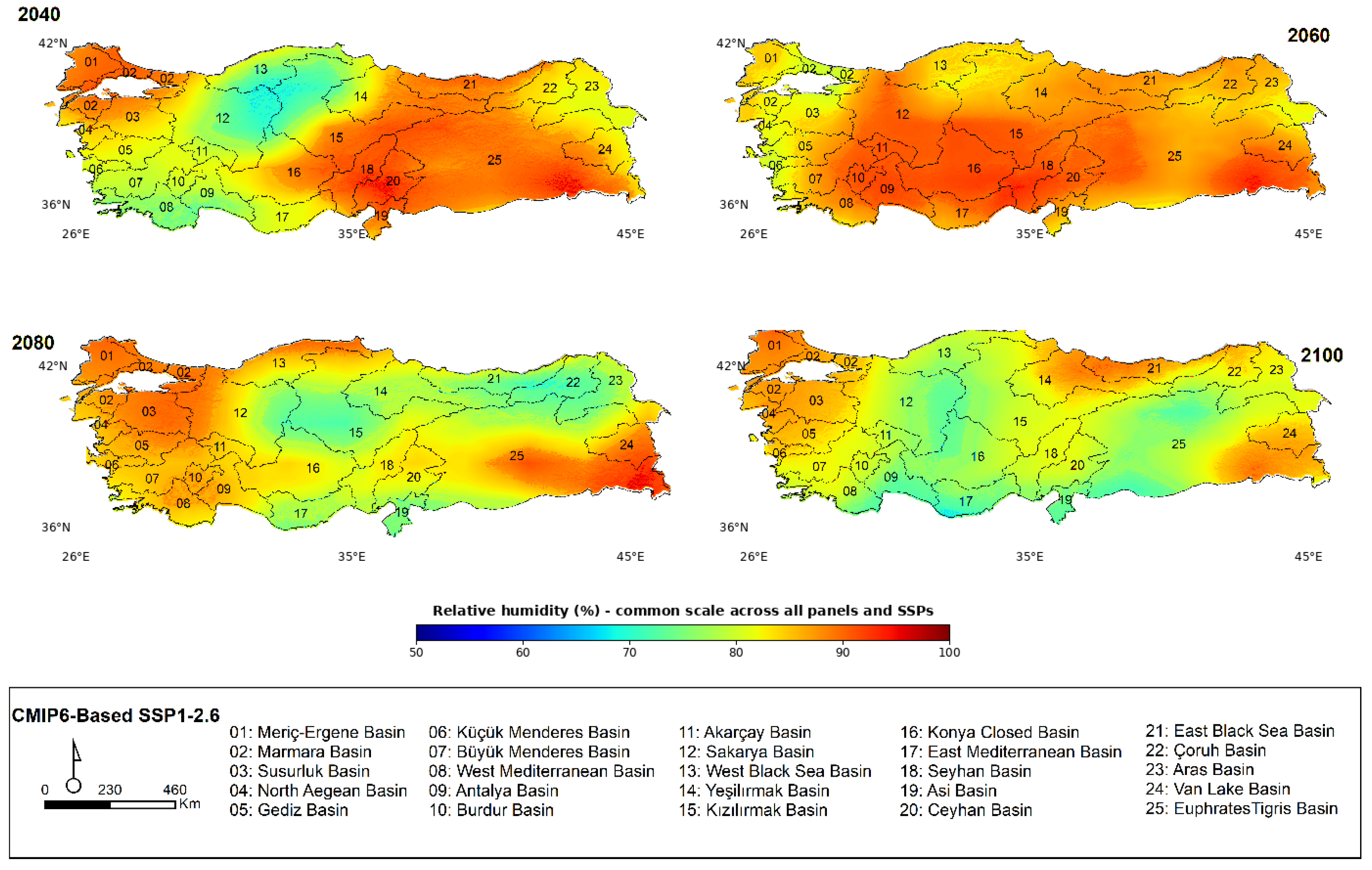
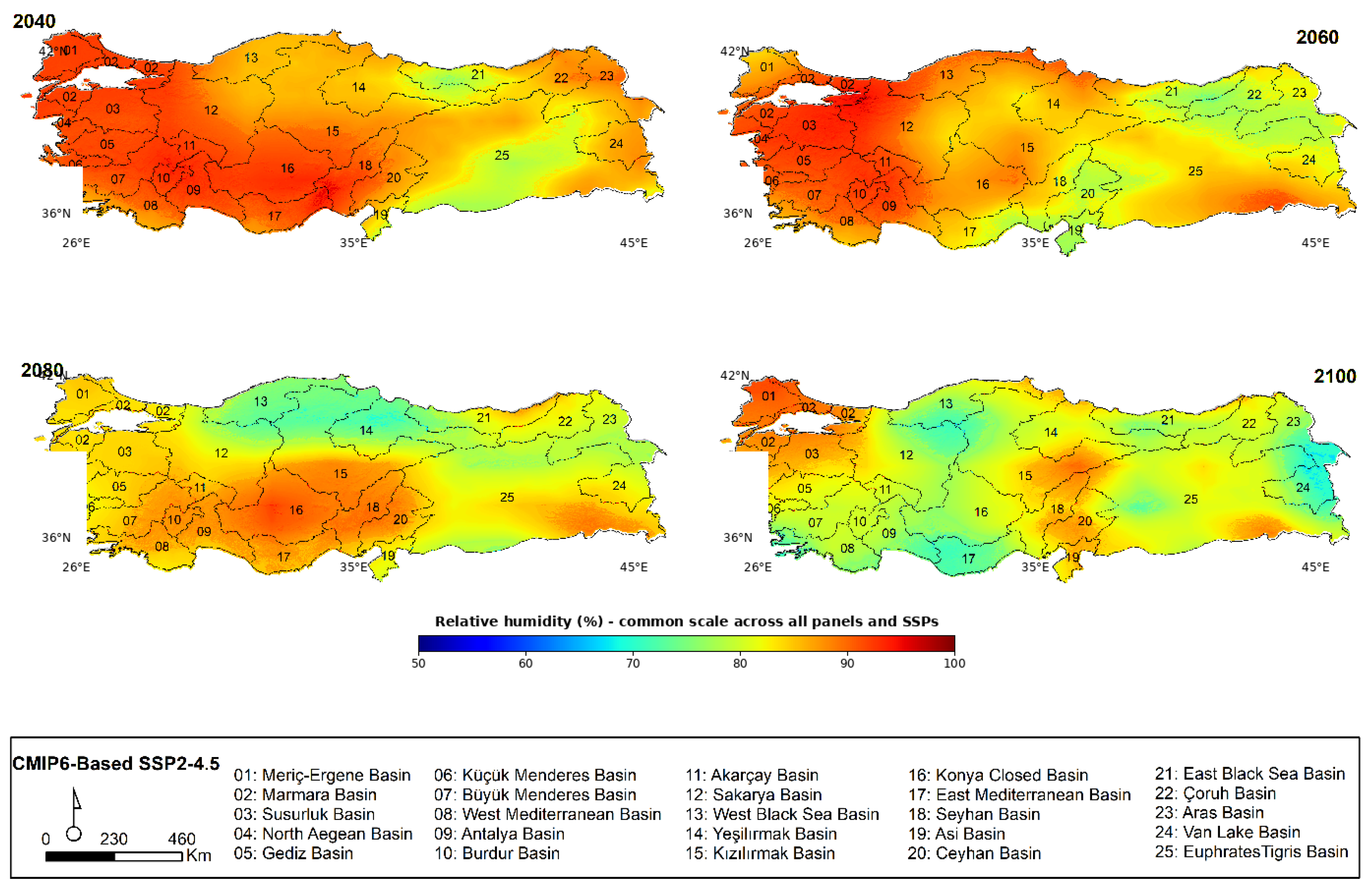
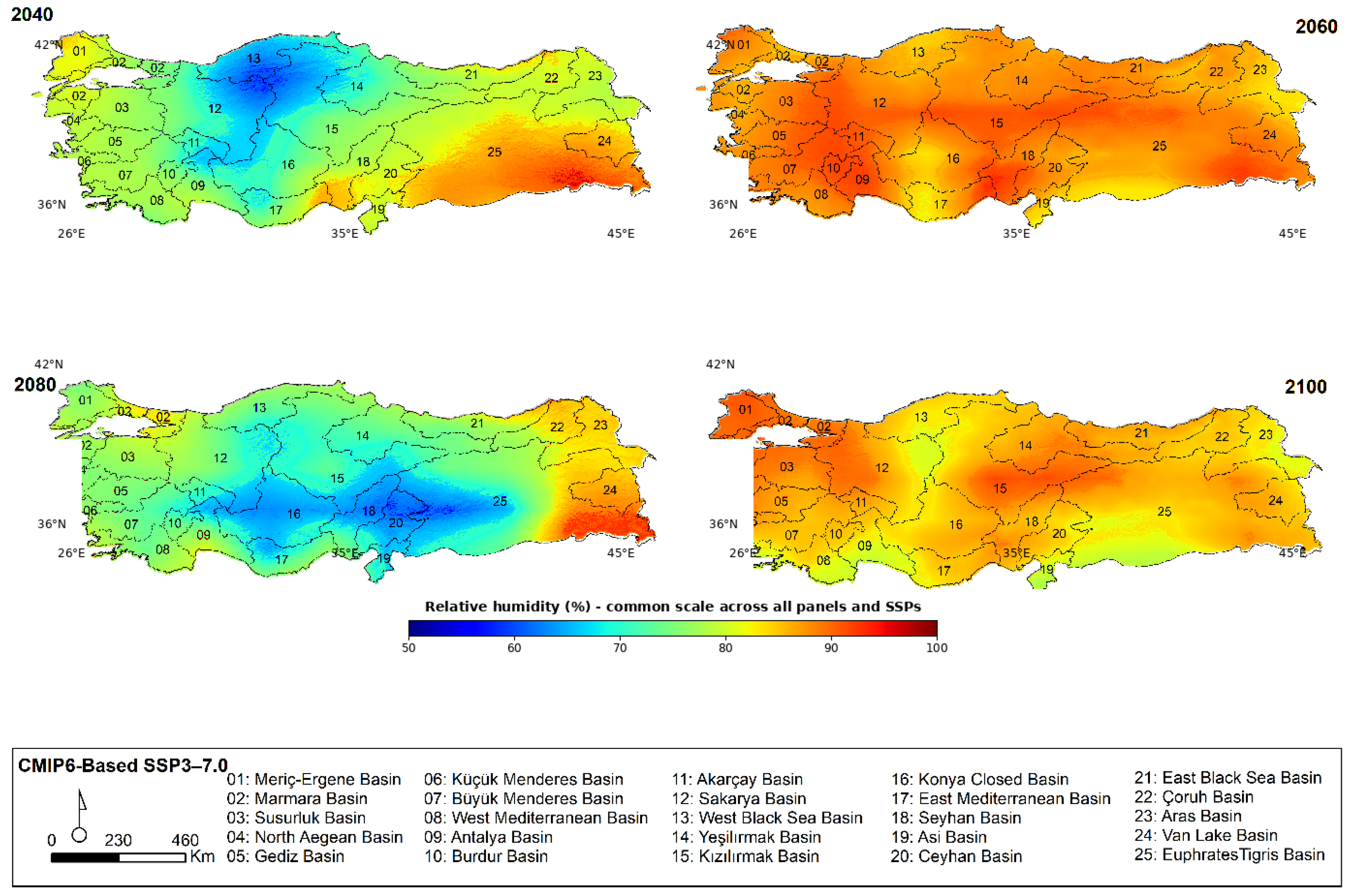
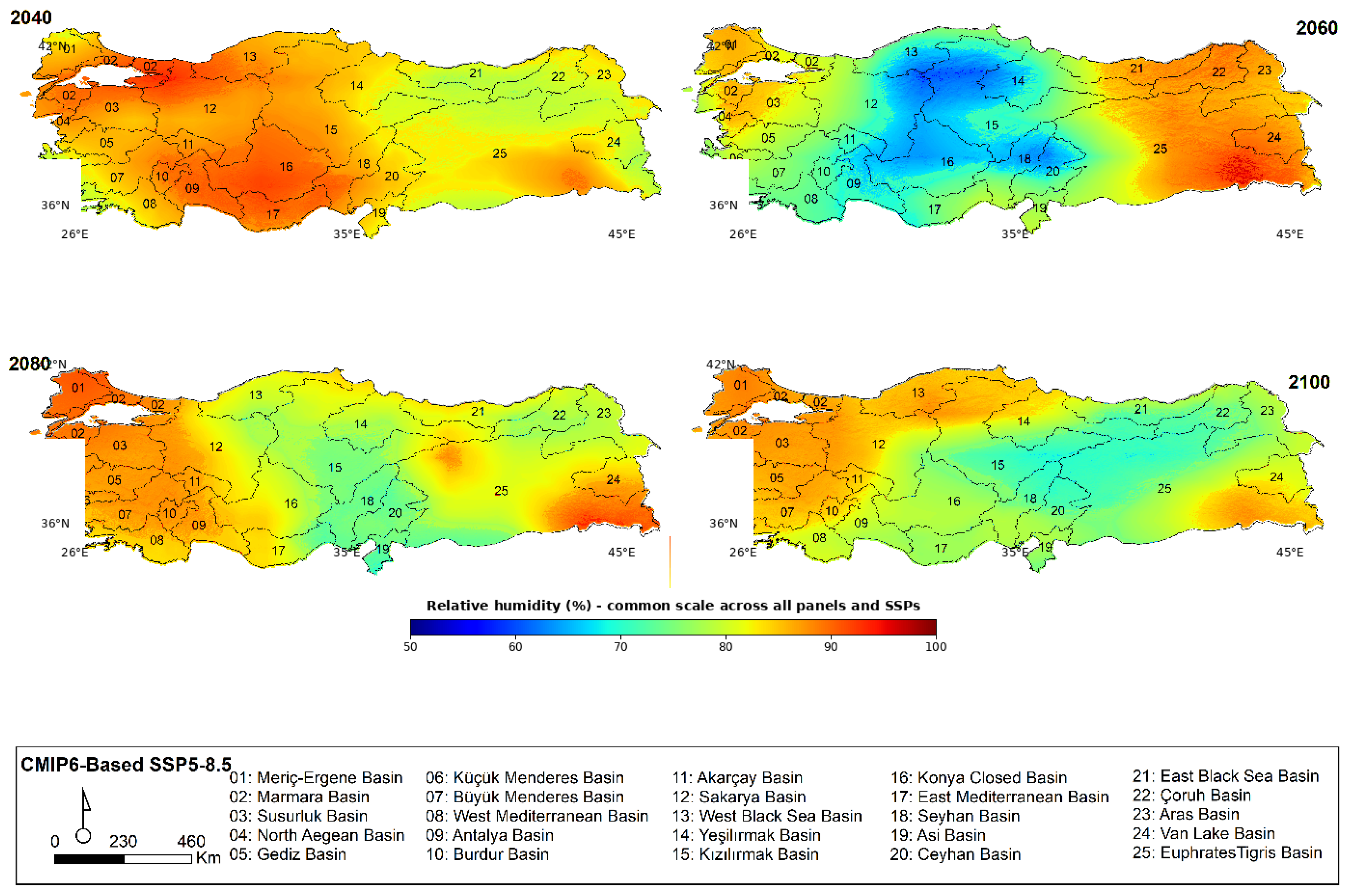
The RH maps show strong spatial heterogeneity among basins and horizons (Figure 2, Figure 3, Figure 4 and Figure 5). The RH maps are displayed with panel-specific color-bar ranges, as indicated by the individual color bars, to preserve spatial contrast, and geographic coordinate marks provide a consistent spatial reference. The higher-forcing pathways show pronounced late-century spatial contrasts, but the single-year horizons should not be interpreted as climatological normals.

3.2. Basin-Scale NDVI–RH Sensitivity

Table 2. Basin-scale scenario-specific NDVI–RH sensitivity indices and descriptive cross-scenario diagnostics. $\overline{\left|\beta \right|}$ is mean absolute sensitivity, $\widetilde{\left|\beta \right|}$ is median absolute sensitivity, $S{D}_{SSP}$ is the sample standard deviation across the four SSP values, and F is the number of scenarios in which the basin is in the scenario-specific upper quartile of $\left|\beta \right|$. Inferential SE, confidence intervals and p-values are not reported because ${\beta }_{i,s}$ is a finite-change index rather than an OLS parameter estimated from repeated observations.

Basin	SSP1-2.6	SSP2-4.5	SSP3-7.0	SSP5-8.5	Mean $\left|\mathit{\beta }\right|$	Median $\left|\mathit{\beta }\right|$	${\mathbf{SD}}_{\mathbf{SSP}}$	F
01: Meric-Ergene	0.0240	0.0061	−0.0146	0.0337	0.0196	0.0193	0.0213	0/4
02: Marmara	0.0374	0.0088	−0.0306	0.0409	0.0294	0.0340	0.0331	1/4
03: Susurluk	−0.0259	0.0145	−0.0324	0.0749	0.0369	0.0292	0.0493	1/4
04: North Aegean	−0.0103	−0.0047	−0.0065	0.0217	0.0108	0.0084	0.0146	0/4
05: Gediz	0.0099	0.0208	−0.0219	0.0286	0.0203	0.0214	0.0222	0/4
06: Küçük Menderes	−0.0448	−0.0531	0.0582	0.0625	0.0547	0.0557	0.0632	4/4
07: Büyük Menderes	−0.0188	−0.0071	0.0062	0.0198	0.0130	0.0130	0.0167	0/4
08: West Mediterranean	0.0065	−0.0029	−0.0084	0.0176	0.0089	0.0075	0.0114	0/4
09: Antalya	0.0374	0.0592	−0.1321	0.0769	0.0764	0.0681	0.0963	4/4
10: Burdur	0.0757	0.0264	0.0293	0.0453	0.0442	0.0373	0.0226	1/4
11: Akarçay	−0.0196	−0.0140	0.0153	0.0349	0.0209	0.0175	0.0256	0/4
12: Sakarya	−0.0280	0.0173	−0.0210	0.0461	0.0281	0.0245	0.0346	1/4
13: West Black Sea	−0.0172	0.0116	−0.0187	0.0299	0.0193	0.0180	0.0236	0/4
14: Yeşilırmak	−0.0206	0.0179	−0.0112	0.0618	0.0279	0.0193	0.0370	1/4
15: Kızılırmak	0.0114	0.0215	−0.0198	0.0268	0.0199	0.0207	0.0209	0/4
16: Konya Closed	0.0540	0.0390	0.1080	0.0399	0.0602	0.0470	0.0326	3/4
17: East Mediterranean	−0.0085	0.0242	−0.0426	0.0239	0.0248	0.0241	0.0318	1/4
18: Seyhan	0.0061	0.0172	−0.0215	0.0224	0.0168	0.0194	0.0196	0/4
19: Asi	−0.0212	0.0106	−0.0284	0.0331	0.0233	0.0248	0.0286	0/4
20: Ceyhan	0.0419	0.0451	0.0196	0.0501	0.0392	0.0435	0.0135	3/4
21: East Black Sea	−0.0149	−0.0120	−0.0178	0.0206	0.0163	0.0164	0.0179	0/4
22: Çoruh	−0.0362	0.0418	−0.0237	0.0485	0.0376	0.0390	0.0437	3/4
23: Aras	0.0162	0.0627	0.0835	0.0455	0.0520	0.0541	0.0285	2/4
24: Van Lake	−0.0089	0.0222	0.0908	0.0296	0.0379	0.0259	0.0417	1/4
25: Euphrates–Tigris	−0.0137	0.0296	0.0589	0.0310	0.0333	0.0303	0.0300	2/4

reports the four scenario-specific sensitivity indices together with descriptive cross-pathway diagnostics. Mean absolute sensitivity summarizes average response magnitude; it is not interpreted as evidence of consistency. Median absolute sensitivity provides a robust central-magnitude check; the across-SSP standard deviation summarizes signed pathway-to-pathway variability, and F gives the number of SSPs in which a basin falls in the scenario-specific upper quartile of absolute sensitivity. These quantities describe the archived matrix and should not be interpreted as regression uncertainty or multi-model climate uncertainty.

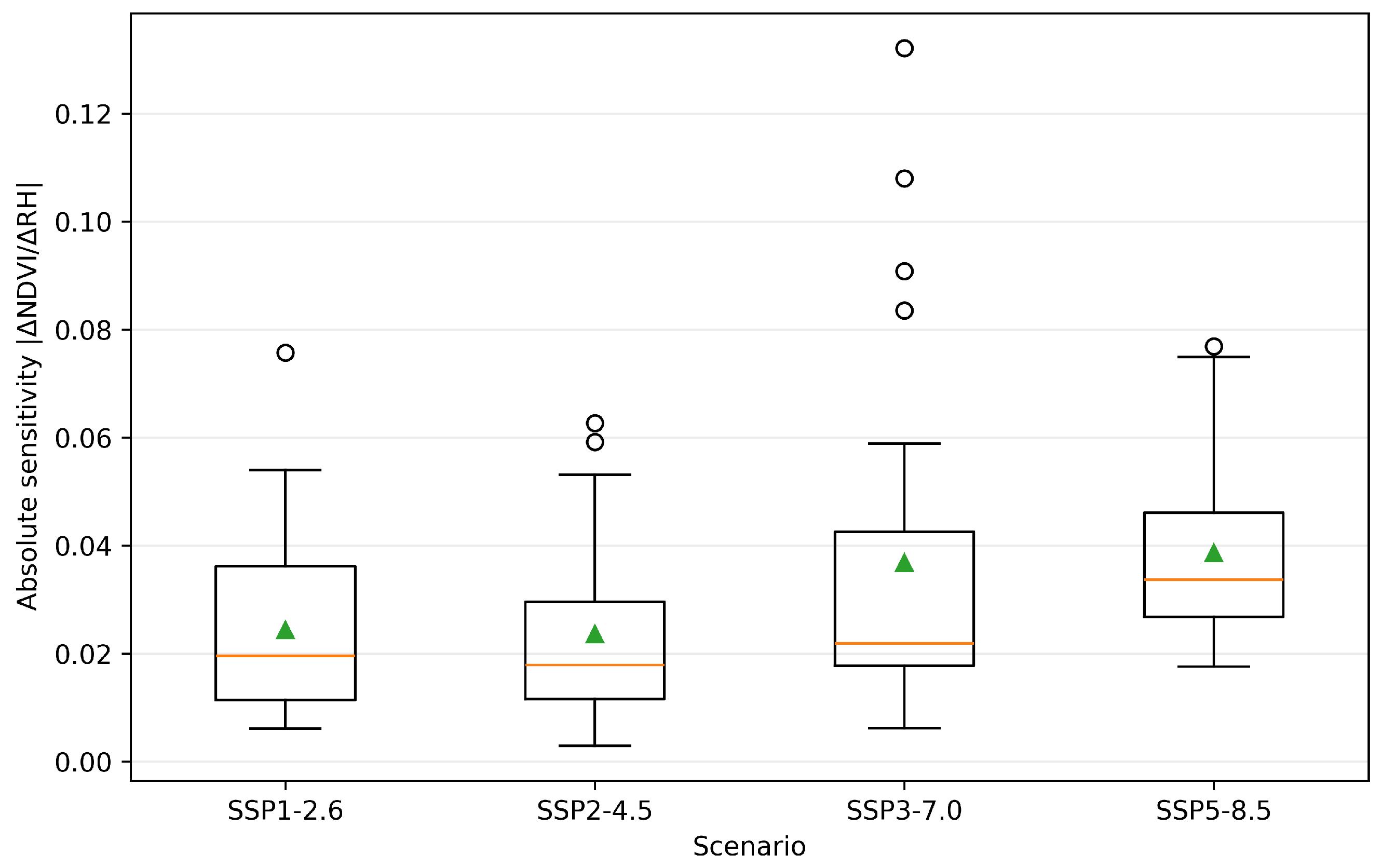
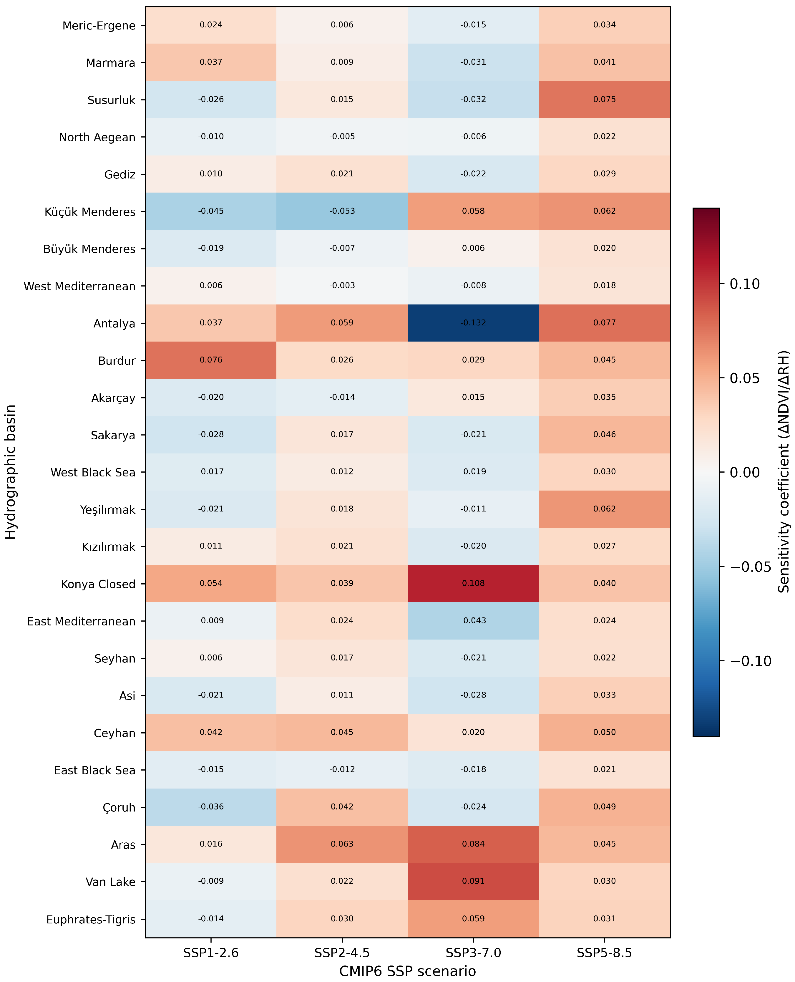
Across basins, mean absolute sensitivity is 0.0244 for SSP1-2.6, 0.0236 for SSP2-4.5, 0.0368 for SSP3-7.0 and 0.0386 for SSP5-8.5. Thus, the two higher-forcing pathways contain the largest overall magnitude of the archived basin index, although individual basins can change sign across scenarios. The heatmap in Figure 6 makes that sign reversal visible. Its diverging color scale is centered on zero; blue indicates negative sensitivity, red indicates positive sensitivity, and the numeric color bar gives the coefficient magnitude.

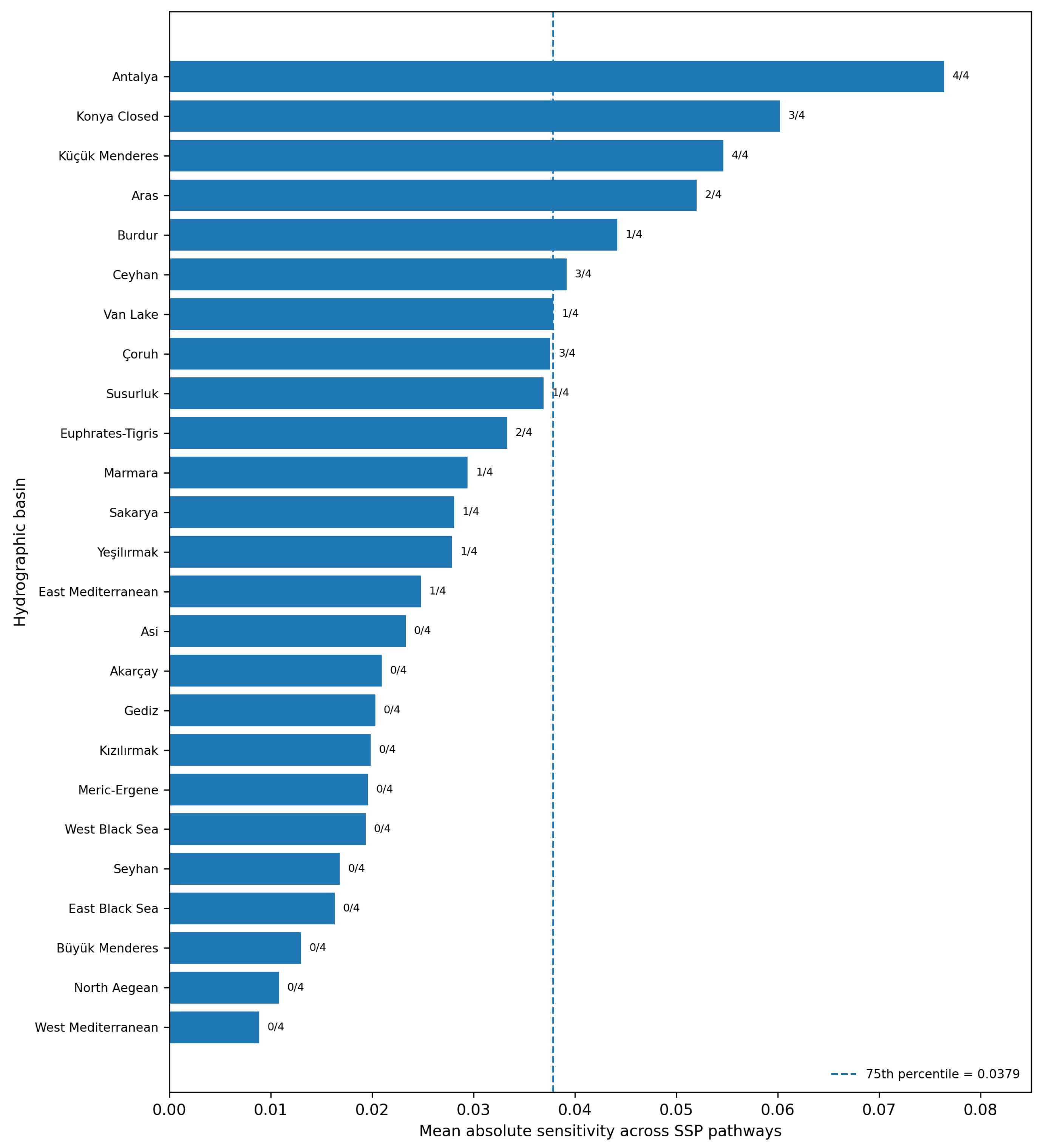
As a robustness check against a single extreme pathway value, median absolute sensitivity was also examined together with the scenario-wise distributions of absolute sensitivity (Figure 7). Its basin-level 75th percentile is 0.0373, and all five basins classified as persistent hotspots by the primary magnitude-plus-persistence rule also exceed this median-magnitude threshold. The basin rankings based on mean and median absolute sensitivity are highly concordant (Spearman rank correlation $\rho =0.947$). This check does not replace a denominator-stability analysis, but it shows that the final persistent-hotspot set is not created solely by one unusually large SSP coefficient.

3.3. Cluster Stability and Response Structure

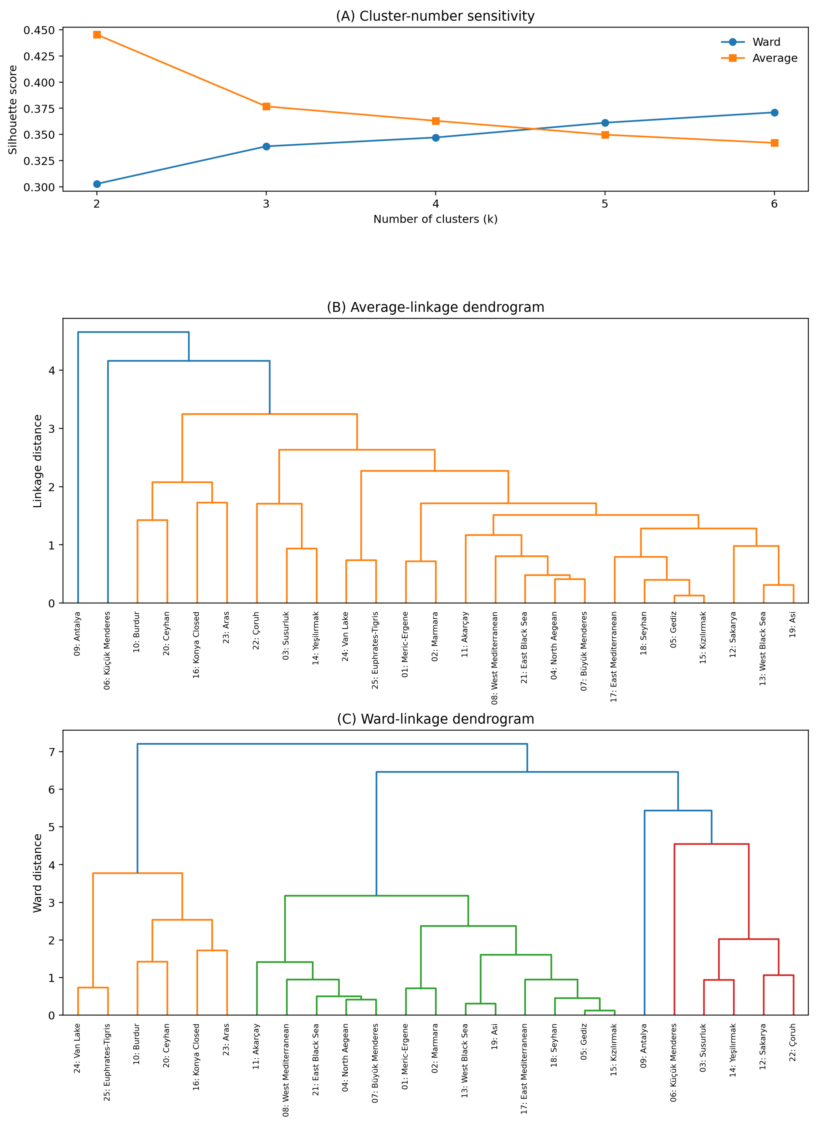
Silhouette diagnostics do not support a uniquely determined three-cluster solution. Average linkage reaches its highest silhouette score at $k=2$ (0.445), whereas Ward linkage increases from 0.303 at $k=2$ to 0.371 at $k=6$ without a clear low-k optimum. The corresponding dendrograms are shown in Figure 8 and are interpreted as exploratory similarity structures rather than as evidence for a fixed ecological typology. Hotspot categories are assigned independently using the quantitative rule in Equation (7).

3.4. Quantitative Hotspot Classification

The 75th percentile of mean absolute basin sensitivity is 0.0379. Five basins satisfy both the magnitude criterion (${\overline{\left|\beta \right|}}_i\ge 0.0379$) and the persistence criterion ($F_i\ge 2$): Antalya, Küçük Menderes, Konya Closed, Ceyhan and Aras (Figure 9;

Table 3. Operational response classes derived reproducibly from the archived sensitivity matrix using the two quantitative hotspot criteria.

Response Class	Basins Meeting the Rule	Operational Definition and Interpretation
Persistent high-response hotspot	Antalya; Küçük Menderes; Konya Closed; Ceyhan; Aras	$\overline{\left|\beta \right|}\ge 0.0379$ and $F\ge 2$. Strong magnitude combined with repeated upper-quartile occurrence. Konya Closed should be interpreted with explicit attention to irrigation and groundwater use.
Transitional/episodic high response	Burdur; Van Lake; Çoruh; Euphrates–Tigris	Exactly one of the two hotspot criteria is met. Sensitivity is either large on average or repeatedly elevated in specific pathways, but not both.
Lower or non-persistent response	Remaining basins	Neither criterion is met in the present coefficient matrix. This does not imply climatic safety; other drivers may dominate the vegetation response.

). Burdur exceeds and Van Lake meets the overall sensitivity threshold, but both do so less persistently, whereas Çoruh and Euphrates–Tigris recur in scenario-specific upper quartiles without exceeding the overall 75th-percentile mean threshold. All five persistent hotspots also exceed the 75th percentile of median absolute sensitivity (0.0373), providing a robust central-magnitude check. The Konya Closed Basin remains a special case because irrigation and groundwater abstraction can maintain greenness independently of natural atmospheric-moisture resilience.

4. Discussion

The basin-scale sensitivity matrix shows substantial spatial heterogeneity, sign reversals across SSPs, and larger overall sensitivity magnitudes under SSP3-7.0 and SSP5-8.5. This behavior is consistent with evidence that vegetation responses to drought depend on atmospheric demand, water availability, biome properties, and drought time scale rather than on a single climatic variable [16,18,33,34].

Lower humidity can increase atmospheric moisture demand and contribute to stomatal closure and reduced productivity, especially where soil-water buffering is limited [14,15,17]. RH nonetheless remains an incomplete physiological metric because VPD also depends strongly on temperature. For that reason, the hotspot classes in Table 3 should be read as RH-associated screening categories. They do not demonstrate that RH independently explains the NDVI response after precipitation, temperature, soil moisture, or management effects are removed.

The quantitative thresholding changes the hotspot interpretation in a useful way. Antalya and Küçük Menderes remain prominent because their average magnitude is high and their upper-quartile occurrence is repeated across all four SSPs. Aras also meets both criteria. Ceyhan combines moderate-to-high coefficients with repeated upper-quartile placement. Konya Closed meets the formal hotspot rule but cannot be interpreted in the same way as a largely rain-fed basin because irrigation and groundwater abstraction can sustain crop greenness while underlying water stress intensifies. The explicit rule therefore improves reproducibility without eliminating the need for basin-specific hydrogeographic interpretation.

Average and Ward linkage do not identify the same unique number of clusters. The dendrograms are therefore most useful as exploratory representations of similarity rather than as a basis for imposing a fixed three-class ecological typology. The percentile-based hotspot rule is independent of cluster choice and can be reproduced directly from Table 2.

Limitations and Priorities for Follow-Up Analysis

Several limitations constrain the strength of inference. First, the processed CMIP6-derived RH products do not retain model/member provenance or the exact historical/reference-period metadata. A genuine multi-model uncertainty envelope therefore cannot be reconstructed from the available products, and cross-SSP variability is reported only as pathway spread. A fully uncertainty-aware reanalysis would retain each GCM and realization separately, apply a common reference period and multi-year climatological windows, propagate the RH anomaly and sensitivity calculation model by model, and summarize the resulting distribution using the ensemble median together with an interquartile range or another documented spread measure.

Second, basin-level harmonization resolves the difference in spatial support between MODIS and the climate-model products but does not constitute climate-model bias correction. The available processing record does not document a model-specific bias-correction or statistical/dynamical downscaling procedure. In addition, the 2040, 2060, 2080 and 2100 products are single-year horizons. They can contain substantial internal variability and should not be interpreted as stable climatological normals. Multi-year windows would be preferable in a regenerated climate-impact analysis.

Third, the archived sensitivity matrix is not a validated predictive model. A predictive use of RH to estimate NDVI would require a time-aligned historical RH–NDVI dataset, fitting on an earlier calibration period, and evaluating on a later contiguous hold-out using basin-wise RMSE, MAE, and out-of-sample $R^2$. MAPE may be secondary because NDVI values near zero can destabilize percentage errors. The required historical RH series is not available in the retained research materials, so no predictive-error statistic is reported, and no future-NDVI prediction is presented as a validated result.

Fourth, the long-term NDVI summary and single-year RH horizons cannot resolve seasonal vegetation dynamics. A time-resolved analysis should estimate the RH–NDVI relationship within basin-specific vegetation-active periods, evaluate lag-0, lag-1, and lag-2 associations, and account for agricultural crop calendars where appropriate. This is especially important in irrigated basins, where management can shift both the magnitude and timing of greenness responses.

Finally, the sensitivity matrix is univariate with respect to atmospheric moisture. Temperature, precipitation, VPD, soil moisture, radiation, CO₂, land-cover change, irrigation, and groundwater use are not jointly estimated. A follow-up multivariable analysis should use aligned time series and report standardized or partial RH effects together with multicollinearity diagnostics. Until those analyses are available, the present hotspot classes should be interpreted as RH-associated screening categories rather than evidence that RH independently drives vegetation change.

5. Conclusions

Basin-scale NDVI–RH sensitivity varies markedly across Türkiye and across the four SSP pathways. Mean absolute sensitivity is larger under SSP3-7.0 and SSP5-8.5 than under SSP1-2.6 and SSP2-4.5. The two-criterion hotspot rule identifies Antalya, Küçük Menderes, Konya Closed, Ceyhan and Aras as persistently high-response basins, whereas Burdur, Van Lake, Çoruh and Euphrates–Tigris show transitional or episodic high sensitivity. Silhouette diagnostics do not support a unique three-class clustering solution, which favors explicit percentile-based response categories over an imposed cluster count.

The findings are most appropriately used for basin prioritization and comparative screening. MODIS provides the observed vegetation baseline, whereas the RH layers are processed climate-model scenario products and the pathway-level sensitivity matrix is treated as a derived screening input rather than a calibrated predictive model. Model-resolved CMIP6 uncertainty, historical hindcast error, denominator stability, seasonal and lagged sensitivity, and multivariable attribution require source data that are not available in the present analysis materials. Future work that restores those data and incorporates precipitation, temperature, VPD, soil moisture, and water-management variables would provide a stronger basis for climate-impact attribution and adaptation planning.

References

1. Giorgi, F.; Lionello, P. Climate change projections for the Mediterranean region. Glob. Planet. Change 2008, 63, 90–104. [Google Scholar] [CrossRef] [Scilit]
2. IPCC. Climate Change 2021: The Physical Science Basis; Contribution of Working Group I to the Sixth Assessment Report of the Intergovernmental Panel on Climate Change; Cambridge University Press: Cambridge, UK; New York, NY, USA, 2021. [Google Scholar] [CrossRef] [Scilit]
3. Malhi, Y.; Franklin, J.; Seddon, N.; Solan, M.; Turner, M.G.; Field, C.B.; Knowlton, N. Climate change and ecosystems: Threats, opportunities and solutions. Philos. Trans. R. Soc. B 2020, 375, 20190104. [Google Scholar] [CrossRef] [Scilit]
4. Matthews, H.D.; Weaver, A.J.; Meissner, K.J.; Gillett, N.P.; Eby, M. Natural and anthropogenic climate change: Incorporating historical land cover change, vegetation dynamics and the global carbon cycle. Clim. Dyn. 2004, 22, 461–479. [Google Scholar] [CrossRef] [Scilit]
5. Woodward, F.I.; Lomas, M.R. Vegetation dynamics: Simulating responses to climatic change. Biol. Rev. 2004, 79, 643–670. [Google Scholar] [CrossRef] [Scilit]
6. Beck, P.S.A.; Atzberger, C.; Høgda, K.A.; Johansen, B.; Skidmore, A.K. Improved monitoring of vegetation dynamics at very high latitudes: A new method using MODIS NDVI. Remote Sens. Environ. 2006, 100, 321–334. [Google Scholar] [CrossRef] [Scilit]
7. Gamon, J.A.; Field, C.B.; Goulden, M.L.; Griffin, K.L.; Hartley, A.E.; Joel, G.; Penuelas, J.; Valentini, R. Relationships between NDVI, canopy structure, and photosynthesis in three Californian vegetation types. Ecol. Appl. 1995, 5, 28–41. [Google Scholar] [CrossRef] [Scilit]
8. Ichii, K.; Kawabata, A.; Yamaguchi, Y. Global correlation analysis for NDVI and climatic variables and NDVI trends: 1982–1990. Int. J. Remote Sens. 2002, 23, 3873–3878. [Google Scholar] [CrossRef] [Scilit]
9. Lu, L.; Kuenzer, C.; Wang, C.; Guo, H.; Li, Q. Evaluation of three MODIS-derived vegetation index time series for dryland vegetation dynamics monitoring. Remote Sens. 2015, 7, 7597–7614. [Google Scholar] [CrossRef] [Scilit]
10. Hao, F.; Zhang, X.; Ouyang, W.; Skidmore, A.K.; Toxopeus, A.G. Vegetation NDVI linked to temperature and precipitation in the upper catchments of Yellow River. Environ. Model. Assess. 2012, 17, 389–398. [Google Scholar] [CrossRef] [Scilit]
11. Lamchin, M.; Lee, W.K.; Jeon, S.W.; Wang, S.W.; Lim, C.H.; Song, C.; Sung, M. Long-term trend and correlation between vegetation greenness and climate variables in Asia based on satellite data. Sci. Total Environ. 2018, 618, 1089–1095. [Google Scholar] [CrossRef] [Scilit]
12. Li, P.; Wang, J.; Liu, M.; Xue, Z.; Bagherzadeh, A.; Liu, M. Spatio-temporal variation characteristics of NDVI and its response to climate on the Loess Plateau from 1985 to 2015. CATENA 2021, 203, 105331. [Google Scholar] [CrossRef] [Scilit]
13. Xu, Y.; Dai, Q.Y.; Zou, B.; Xu, M.; Feng, Y.X. Tracing climatic and human disturbance in diverse vegetation zones in China: Over 20 years of NDVI observations. Ecol. Indic. 2023, 152, 111170. [Google Scholar] [CrossRef] [Scilit]
14. Allen, R.G.; Pereira, L.S.; Raes, D.; Smith, M. Crop Evapotranspiration: Guidelines for Computing Crop Water Requirements; FAO Irrigation and Drainage Paper 56; Food and Agriculture Organization of the United Nations: Rome, Italy, 1998. [Google Scholar]
15. López, J.; Way, D.A.; Sadok, W. Systemic effects of rising atmospheric vapor pressure deficit on plant physiology and productivity. Glob. Change Biol. 2021, 27, 1704–1720. [Google Scholar] [CrossRef] [Scilit]
16. Novick, K.A.; Ficklin, D.L.; Stoy, P.C.; Williams, C.A.; Bohrer, G.; Oishi, A.C.; Papuga, S.A.; Phillips, R.P. The increasing importance of atmospheric demand for ecosystem water and carbon fluxes. Nat. Clim. Chang. 2016, 6, 1023–1027. [Google Scholar] [CrossRef] [Scilit]
17. Wen, R.; Jiang, P.; Qin, M.; Jia, Q.; Cong, N.; Wang, X.; Meng, Y.; Chen, N. Regulation of NDVI and ET negative responses to increased atmospheric vapor pressure deficit by water availability in global drylands. Front. For. Glob. Change 2023, 6, 1164347. [Google Scholar] [CrossRef] [Scilit]
18. Yuan, W.; Zheng, Y.; Piao, S.; Ciais, P.; Lombardozzi, D.; Wang, Y.; Ryu, Y.; Yang, S. Increased atmospheric vapor pressure deficit reduces global vegetation growth. Sci. Adv. 2019, 5, eaax1396. [Google Scholar] [CrossRef] [Scilit]
19. Eyring, V.; Bony, S.; Meehl, G.A.; Senior, C.A.; Stevens, B.; Stouffer, R.J.; Taylor, K.E. Overview of the Coupled Model Intercomparison Project Phase 6 (CMIP6) experimental design and organization. Geosci. Model Dev. 2016, 9, 1937–1958. [Google Scholar] [CrossRef] [Scilit]
20. Gidden, M.J.; Riahi, K.; Smith, S.J.; Fujimori, S.; Luderer, G.; Kriegler, E.; van Vuuren, D.P.; Takahashi, K. Global emissions pathways under different socioeconomic scenarios for use in CMIP6: A dataset of harmonized emissions trajectories through the end of the century. Geosci. Model Dev. 2019, 12, 1443–1475. [Google Scholar] [CrossRef] [Scilit]
21. Meinshausen, M.; Nicholls, Z.R.J.; Lewis, J.; Gidden, M.J.; Vogel, E.; Freund, M.; Beyerle, U.; Vollmer, M.K. The shared socio-economic pathway (SSP) greenhouse gas concentrations and their extensions to 2500. Geosci. Model Dev. 2020, 13, 3571–3605. [Google Scholar] [CrossRef] [Scilit]
22. O’Neill, B.C.; Tebaldi, C.; van Vuuren, D.P.; Eyring, V.; Friedlingstein, P.; Hurtt, G.; Knutti, R.; Sanderson, B.M. The Scenario Model Intercomparison Project (ScenarioMIP) for CMIP6. Geosci. Model Dev. 2016, 9, 3461–3482. [Google Scholar] [CrossRef] [Scilit]
23. Tebaldi, C.; Debeire, K.; Eyring, V.; Fischer, E.; Fyfe, J.; Friedlingstein, P.; Knutti, R.; Ziehn, T. Climate model projections from the Scenario Model Intercomparison Project (ScenarioMIP) of CMIP6. Earth Syst. Dyn. 2021, 12, 253–293. [Google Scholar] [CrossRef] [Scilit]
24. Su, B.; Huang, J.; Mondal, S.K.; Zhai, J.; Wang, Y.; Wen, S.; Gao, M.; Li, A. Insight from CMIP6 SSP-RCP scenarios for future drought characteristics in China. Atmos. Res. 2021, 250, 105375. [Google Scholar] [CrossRef] [Scilit]
25. Wei, Y.; She, D.; Xia, J.; Wang, G.; Zhang, Q.; Huang, S.; Zhang, Y.; Wang, T. Climate change dominates the increasing exposure of global population to compound heatwave and humidity extremes in the future. Clim. Dyn. 2024, 62, 6203–6217. [Google Scholar] [CrossRef] [Scilit]
26. Zhou, Z.; Zhang, L.; Chen, J.; She, D.; Wang, G.; Zhang, Q.; Xia, J.; Zhang, Y. Projecting global drought risk under various SSP-RCP scenarios. Earth’s Future 2023, 11, e2022EF003420. [Google Scholar] [CrossRef] [Scilit]
27. Vicente-Serrano, S.M.; Domínguez-Castro, F.; Beguería, S.; El Kenawy, A.; Gimeno-Sotelo, L.; Franquesa, M.; Azorin-Molina, C.; Halifa-Marín, A. Atmospheric drought indices in future projections. Nat. Water 2025, 3, 374–387. [Google Scholar] [CrossRef] [Scilit]
28. Didan, K. MOD13A1 MODIS/Terra Vegetation Indices 16-Day L3 Global 500 m SIN Grid V061 [Dataset]. NASA EOSDIS Land Processes DAAC; 2021. Available online: https://www.earthdata.nasa.gov/data/catalog/lpcloud-mod13a1-061 (accessed on 23 June 2026).
29. Huete, A.; Didan, K.; Miura, T.; Rodriguez, E.P.; Gao, X.; Ferreira, L.G. Overview of the radiometric and biophysical performance of the MODIS vegetation indices. Remote Sens. Environ. 2002, 83, 195–213. [Google Scholar] [CrossRef] [Scilit]
30. Amani, M.; Ghorbanian, A.; Ahmadi, S.A.; Kakooei, M.; Moghimi, A.; Mirmazloumi, S.M.; Brisco, B. Google Earth Engine cloud computing platform for remote sensing big data applications: A comprehensive review. IEEE J. Sel. Top. Appl. Earth Obs. Remote Sens. 2020, 13, 5326–5350. [Google Scholar] [CrossRef] [Scilit]
31. Gorelick, N.; Hancher, M.; Dixon, M.; Ilyushchenko, S.; Thau, D.; Moore, R. Google Earth Engine: Planetary-scale geospatial analysis for everyone. Remote Sens. Environ. 2017, 202, 18–27. [Google Scholar] [CrossRef] [Scilit]
32. Zhao, Q.; Yu, L.; Li, X.; Peng, D.; Zhang, Y.; Gong, P. Progress and trends in the application of Google Earth and Google Earth Engine. Remote Sens. 2021, 13, 3778. [Google Scholar] [CrossRef] [Scilit]
33. Vicente-Serrano, S.M.; Gouveia, C.; Camarero, J.J.; Beguería, S.; Trigo, R.; López-Moreno, J.I.; Azorín-Molina, C.; Sanchez-Lorenzo, A. Response of vegetation to drought time-scales across global land biomes. Proc. Natl. Acad. Sci. USA 2013, 110, 52–57. [Google Scholar] [CrossRef] [Scilit]
34. Grossiord, C.; Buckley, T.N.; Cernusak, L.A.; Novick, K.A.; Poulter, B.; Siegwolf, R.T.W.; Sperry, J.S.; McDowell, N.G. Plant responses to rising vapor pressure deficit. New Phytol. 2020, 226, 1550–1566. [Google Scholar] [CrossRef] [Scilit]
Figure 1. Hydrographic basins of Türkiye used in the analysis. The inset locates Türkiye within the European–Mediterranean domain. The terrain ramp is labeled as elevation (m), and geographic coordinate marks provide spatial reference.
Climate 14 00179 g001
Figure 2. Projected RH distribution (%) under SSP1-2.6 at the 2040, 2060, 2080, and 2100 single-year horizons. The individual panels use panel-specific RH color-bar ranges, as indicated by their color bars.
Climate 14 00179 g002
Figure 3. Projected RH distribution (%) under SSP2-4.5 at the 2040, 2060, 2080, and 2100 single-year horizons, shown with panel-specific RH color-bar ranges indicated by the individual color bars.
Climate 14 00179 g003
Figure 4. Projected RH distribution (%) under SSP3-7.0 at the 2040, 2060, 2080 and 2100 single-year horizons, shown with panel-specific RH color-bar ranges indicated by the individual color bars.
Climate 14 00179 g004
Figure 5. Projected RH distribution (%) under SSP5-8.5 at the 2040, 2060, 2080 and 2100 single-year horizons, shown with panel-specific RH color-bar ranges indicated by the individual color bars.
Climate 14 00179 g005
Figure 6. Basin-scale NDVI–RH sensitivity indices across four SSP pathways. The numeric color bar maps signed coefficient magnitude, with zero as the neutral midpoint.
Climate 14 00179 g006
Figure 7. Scenario-wise distribution of absolute NDVI–RH sensitivity across the 25 hydrographic basins. Horizontal lines denote medians, green triangles denote means, and open circles denote outliers.
Climate 14 00179 g007
Figure 8. Cluster-number sensitivity and hierarchical similarity structure. (A) Silhouette coefficients for Ward and Average linkage for k = 2 –6. (B) Average-linkage dendrogram with linkage distance on the vertical axis. (C) Ward-linkage dendrogram with Ward distance on the vertical axis.
Climate 14 00179 g008
Figure 9. Mean absolute NDVI–RH sensitivity across SSPs for the 12 highest-ranked basins. Bars are ordered from highest to lowest mean absolute sensitivity. Complete values for all 25 basins, including the SSP-specific upper-quartile occurrence count (F), are reported in Table 2.
Climate 14 00179 g009