Climate Change in the Middle East and the West Indian Subcontinent: Geographic Interconnections and the Modulation Roles of the Extreme Phases of the Atlantic Meridional Oscillation (AMO) and the Monsoon Cloudiness

Abstract

In this study, the long-term (1961–2020) values of the summertime station-based surface air temperature (SAT) data at 151 qualified stations, alongside the corresponding ERA5 gridded data, were analyzed to investigate climate change over the Middle East and the west Indian subcontinent. Significant positive (negative) trends were observed at 134 (2) stations, while trends were insignificant at 15 stations. The positive (negative and insignificant) trends were mainly concentrated in the interior highlands (monsoon-dominated lowlands), where ERA5 exhibited from 10% to 70% overestimations (5% to 26% underestimations). These ERA5-related biases exhibited strong correlations with elevation. To assess the trends’ disparity reasons, we first showed that the outputs of SAT_+AMO − SAT_−AMO are highly positive (negative or near zero) over the overestimated (underestimated) regions. The study then demonstrated that cloudiness, atmospheric circulation, specific humidity, and convective activities above the monsoon-dominated areas differ between +AMO and −AMO. For these areas, the enhanced +AMO-related cloudiness suppresses positive SAT anomalies, while the increased −AMO-associated sunshine offsets negative SAT anomalies. Contrarily, for some areas such as northern Iran, the +AMO (−AMO)-associated cloudiness or clear sky can affect climate change by amplifying the warmness or coldness. In addition, +AMO (−AMO) has caused further convective activities over the Arabian Sea (Bengal Bay).

1. Introduction

Climate change, particularly the warming trend throughout the twenty-first century, is a global phenomenon and the inevitable process that imposes significant impacts on various ecosystems and human societies worldwide [1,2]. Some of these impacts include an increase in natural hazards [3,4], accelerated hydrologic and carbon cycles [5], reduced food security [6,7], the geographic expansion of many infectious diseases [8,9], and a range of adverse economic and health effects [10,11,12,13,14]. Quantifying the measures of climate change is essential for implementing adaptation strategies, policy-making, resource management, resilience enhancement, and mitigating the negative impacts of such changes.

While other weather elements such as precipitation, pressure, and humidity are important, surface air temperature (SAT) serves as the basis for assessing all other weather elements, both directly and indirectly. This atmospheric component plays an influential role in both natural systems and human lives and activities, such as health, agriculture, energy and more. As a key indicator of climate change, SAT is vital for understanding the global atmospheric and oceanic circulations and assessing hazard risk [15,16,17,18]. Notably, compared to other seasons, the increase in global temperature is more pronounced during summertime [19], leading to extreme weather conditions worldwide [20].

Middle Eastern countries have experienced a significant warming trend characterized by longer and warmer summers, drier climate, and increased frequency and severity of heat waves [21]. Although statistical changes in meteorological and climate features are a worldwide threat, the Middle East (ME), identified as a global climate change hotspot [22,23], has experienced significant changes in SAT data. For example, an analysis of annual mean temperature extremes in 50 meteorological stations in various parts of Iran showed a significant upward trend from 1975 to 2010 [24]. Due to its unique geographic and environmental characteristics, the ME is expected to face more adverse effects of climate change such as increased water demand and further ecosystem degradation. Similarly, heat waves have shown a positive trend in North, Northwest, and Central India [25,26,27].

Long-term time series of observed SAT data are essential for directly evaluating climate change and assessing bias in the model-based time series. However, the scarcity of long-term records with acceptable spatial coverage limits their application. These limitations are particularly critical in some areas, such as the ME, where observed records have low temporal-spatial resolution. For example, biases in the model’s mean or maximum temperature were assessed for India [28], revealing the highest cold bias in South Peninsular India and maximum precipitation bias in the Northeast.

The parallel utilization of the observed and the model-based datasets, accompanied by bias correction procedures, can reduce the errors in climate analysis. Accordingly, we used SAT data from both datasets to explore climate change over the ME and the west Indian subcontinent. Comparing the results provided by these datasets allowed us to gain insights into model biases and their impacts on climate change analysis [29]. Comparing the spatial distributions of magnitudes of changes led us to conclude that several teleconnections modulate these changes. Notably, in addition to the direct impacts of global warming, our study area is also influenced by regional climate patterns, including the El Niño Southern Oscillation (ENSO) [30,31,32], the North Atlantic Oscillation (NAO) [33,34], the Madden Julian Oscillation (MJO) [35,36], the Atlantic Meridional Oscillation (AMO) [37], and the Monsoon [38]. Among these well-known teleconnections, after some preliminary examinations, assessing important aspects of the SAT–AMO-monsoon relationships over the study area was considered as one of the main themes of this study.

The AMO is characterized by a sequence of long-term fluctuations in sea surface temperature (SST) across the North Atlantic Ocean, typically from 0° to 80° N. The cool and warm phases of this phenomenon may last for 20–40 years, with a temperature differential of approximately 1° F between the extremes [39]. The AMO influences mean SAT [40,41] and rainfall across the Northern Hemisphere, in particular North America and Europe [42,43]. The warm phase of the AMO influences the monsoon through the Summer North Atlantic Oscillation (SNAO) and also through the equatorial zonal winds [44]. Some investigations have shown the impact of different phases of the Atlantic Multidecadal Oscillation (AMO) on atmospheric variations and precipitation, emphasizing that the warm phase of the AMO is typically associated with heightened storm activity and heavier rainfall in monsoon-dependent regions [45]. Another study presented evidence that the warm phase of the AMO was correlated with enhanced monsoon activity in Asia. This correlation was particularly evident during certain decades, where increased sea surface temperatures in the Atlantic coincide with stronger monsoon rainfall in regions such as India and Southeast Asia [46]. Recent investigations into Indian heatwaves have highlighted their intricate relationship with climatic factors. Ratnam et al. (2016) conducted a comprehensive study on the anatomy of Indian heatwaves, revealing significant correlations with broader climate phenomena [47]. Complementing this, Sahu et al. (2020) explored the impacts of Indo-Pacific climate variability on rice productivity in Bihar, emphasizing how climate teleconnections significantly affect agricultural outputs [48]. Additionally, this phenomenon reflects the more important characteristics of heat flux in the surface and subsurface of the North Atlantic Ocean [49,50]. Moreover, the AMO is interconnected with several other teleconnections that could influence climate conditions over the ME and Indian subcontinent, including the El Niño Southern Oscillation (ENSO) [51], the Pacific Decadal Oscillation (PDO) [52], the Pacific/North America (PNA) [53,54], and the equatorial Pacific decadal variability [55].

Despite the AMO being one of the primary drivers of the Earth’s climate system, its modulation role concerning the monsoon and climate change has received relatively little attention [56,57]. Notably, global warming has shortened monsoonal activities in several regions across the Indian Subcontinent [58]. This means an increase in long dry periods with low or no rainfall, intermittent with short but intense spells of rainfall. These changes are particularly significant in India’s western, central, and eastern states, where more than 55% of the cultivated area is largely rain-fed and the adaptive capacity is the lowest. Moreover, the CMIP-5 projected an increasing trend in sub-seasonal variability of the Indian summer monsoon rainfall with increasing global mean temperature [59]. Similarly, During the period of 2010–2017, Pakistan experienced a decreasing trend in monsoon rainfall coupled with an increasing trend in temperature, with these monsoonal patterns being significantly influenced by large-scale circulations such as the Indian Ocean Dipole (IOD) and ENSO [60,61]. Conversely, AMO research investigates long-term climatic oscillations affecting broader regions, which may include direct or indirect influences on monsoonal activities. The East and South Asian monsoons are very important, as they profoundly influence the most densely populated regions in the world (the total population of which exceeds half of the world’s population) [62,63]. Due to such systematic inter-connections between the AMO and monsoonal activities, understanding the combined effects of these two climate components on climate change over these areas is essential for developing effective strategies to adapt to and mitigate the impacts of climate change. We can better inform policy decisions and enhance resilience in vulnerable communities and regions.

The non-parametric Mann-Kendall Test has frequently been used to verify climate change in Iran across various temporal-spatial scales, using different meteorological elements as the climate indicators [64,65,66,67,68]. The air temperature over Saudi Arabia has increased significantly, and the rate is faster (0.72 °C per decade) in the dry season compared to the wet season (0.51 °C per decade). Rainfall has statistically decreased in Saudi Arabia except for the south of the Peninsula, and, in particular, along the Red Sea coast, where rainfall has increased [69].

Model-based datasets offer a significant advantage due to their extensive range of temporal-spatial resolutions, enabling the creation of comprehensive long-term climatologies for various variables without temporal or spatial gaps. The ERA5 reanalysis dataset is particularly valuable in this regard, estimating multiple land surface variables with high spatial and temporal resolutions [70]. The high-resolution (0.25° × 0.25°) ERA5 dataset [71] used in this study allows for the analysis of climate change over a climatically significant period from 1950 to the present, demonstrating its potential in studying climate change [72], storm surge [73], cloud cover [74], atmospheric blocking systems [75,76], and hydro-meteorological hazards [77]. This study leveraged a high-resolution SAT dataset to assess model bias, relating it to elevation and a few climate drivers like the AMO and monsoon.

The United States National Oceanic and Atmospheric Administration (NOAA) provides critical environmental information and forecasts via over one hundred observing systems and numerical models [78]. In this study, NOAA data, along with the ERA5 dataset, were used to improve and validate our findings. Specifically, we compared NOAA-based SAT, outgoing longwave radiation (OLR), omega, specific humidity, and vector wind (VW) at the 500 and 700 hPa levels between +AMO and −AMO. OLR, a proxy for cloud cover, represents the energy radiated from Earth to space and is influenced by surface air temperature, atmospheric temperature, and cloud amount [79].

The informative previous studies have mainly used a variety of methodologies and climate variables to characterize different aspects of climate change in a specific country or region of the Middle East and the Indian subcontinent. However, assessing the interconnections between climate changes over these two regions has not been the themes of their study. Additionally, evaluating the impacts of global or regional climate drivers on the spatial diversity of these areas’ SAT trends has not yet been thoroughly explored. Although numerous investigations have quantified the model-based biases and used various downscaling methods to minimize errors, less attention has been given to explaining the bias sources and introducing possible approaches to improve the models’ accuracy. In other words, the influence of the drivers’ impacts as the source of model bias was mostly overlooked. The lack of such evaluations has hindered the ability of scientific communities to explain the reasons for unevenly distributed SAT trends over the study area.

This study investigated climate change in the Middle East and the west Indian sub-continent using observational and ERA5 datasets. It mapped and classified SAT-based climate change, quantifies ERA5 biases, and assesses bias-topography relationships. The analysis revealed interconnected climate change patterns influenced by geography and global teleconnections, highlighting trend differences between coastal lowlands and interior highlands. The study identified regions where the extreme AMO phases statistically change SAT values, proving the forcing effects of the AMO on climate change. Furthermore, it explored the interactions between extreme AMO phases and monsoon-related phenomena, providing a new physical explanation for climate change and clarifying the influence of AMO and monsoon interactions on spatial SAT trend variations. The assessment of how extreme AMO phases shift monsoon activity centers and the sensitivity test to validate results across different AMO thresholds strengthened the findings. These results are expected to significantly contribute to more effective climate change mitigation strategies and to develop more accurate model-based SAT data.

2. Materials and Methods

Our data sources include the following:

• The monthly (June-September) surface air temperature (SAT) data of 151 meteorological stations spread over various parts of the ME and Indian subcontinent (1961–2020), which were gratefully extracted from the webpage of the National Aeronautics and Space Administration Goddard Institute for Space Studies (NASA) [80]. To ensure the best temporal-spatial coverage, the stations were selected according to the availability and quality of data. Besides the country and station name, Table S1 shows the elevation (column 3) and some statistical properties of the station-based datasets. These properties mainly include the mean SAT values over the study period for the observed and the ERA5-related datasets, the mean anomalies of SAT data during +AMO and −AMO, and the bias-related statistics.
• To resolve the missing data problems in some stations, such as Baghdad, Najaf, and Mosul in Iraq, we gratefully used the webpage of the State Meteorological Agency of Spain [81] to fill the missed values and improve the results’ consistency.
• The ERA5-based gridded SAT data with 0.25° × 0.25° resolution, obtained from the official website of the European Centre for Medium-Range Weather Forecasts (ECMWF), were another source of the data used [82]. Besides using these datasets for assessing climate change, these gridded datasets were also utilized to compensate for the temporal-spatial deficiencies in the observed datasets, including missing values and spatial coverage inadequacies.
• The June-September monthly values of the AMO, extracted from the NOAA webpage.
• The NOAA-based values of several atmospheric variables with the resolution of 2.5° × 2.5° were obtained through the application of monthly–seasonal composites [83]. These variables included SAT, OLR, the near-surface and mid-atmosphere wind vector, omega, and specific humidity at the 500 hPa level. While OLR data were used as the proxy of cloud cover, the mid-atmospheric values of omega and specific humidity served as the proxies of convective activities. Since the interpolated OLR data were available only for the period after 1980, this dataset and corresponding values of AMO, omega, and vector wind were analyzed for the period 1980–2020.

Methods

• Using the arithmetic averaging methods, we initially transferred the monthly (June-September) values of the observed and simulated datasets into their seasonal (summertime) time series [84].
• The non-parametric Mann-Kendall test [85,86] was subsequently used to detect changes in both observed and the ERA5-related SAT data for the period 1961–2020 [87,88]. The significance levels of 0.01, 0.05, and 0.1 were applied to assess the change in the SAT time-series.
• The Kriging method was applied using the ArcGIS 10.7 mapping facilities to show and classify the spatial distribution of the areas with significant or insignificant changes through the generated maps [89]. The choice between different interpolation methods like Kriging, IDW, and Spline, depends on the type of data, specific modeling requirements, and analysis objectives [90]. For data with strong spatial structures, Kriging typically has an advantage, while for simpler applications, IDW and Spline are also suitable options.
• To determine bias in the ERA5 dataset, we subtracted simulated SAT data from the corresponding observed values at 151 meteorological stations (Table S1, column 9). Bias and bias percentage were calculated as follows: Bias = [(SAT_{observed-data} − SAT_modeled-data)] and [Bias% = (100 × Bias)/Observed data], respectively. Positive (negative) bias values indicate the model’s underestimation (overestimation) [91].
• To evaluate the sensitivity of generated maps to interpolation methods, the spatial distribution of bias and other variables was mapped using IDW and Kriging. For example, Figures S1 and S2 illustrate this comparison for BIAS. Kriging more effectively captured extreme values; therefore, all interpolations were performed using Kriging, a technique supported by numerous studies [92,93,94,95,96].
• Aiming for almost a similar number of years in the +AMO and −AMO categories to avoid skewing results toward the more frequent phase, years with summertime AMO index anomalies exceeding +0.15 and falling below −0.15 were classified as the extreme +AMO phases, respectively (

  Table 1. The years of AMO phases (1980–2020), with standardized AMO index anomalies above +0.15 (14 years) and below −0.15 (12 years).

  	Years of +AMO	Years of −AMO
  1	1987	1981
  2	1995	1982
  3	1998	1983
  4	2003	1984
  5	2004	1985
  6	2005	1986
  7	2006	1991
  8	2010	1992
  9	2012	1993
  10	2014	1994
  11	2016	1996
  12	2017	2002
  13	2019
  14	2020

  ). The selected thresholds categorize approximately 35%, 30%, and 35% of the 40-year period as +AMO, −AMO, and normal AMO states, which are found suitable after testing alternatives. For example, raising the threshold to ±0.2 increased +AMO years to 21 (over 50% of the period) while leaving −AMO years unchanged. Since the interpolated OLR data has been available for periods after 1980, this table shows the years from 1980 to 2020. Except for the Mann-Kendall test, the other analyses primarily focused on this period. Properly defining thresholds such as ±0.2 °C not only aids in identifying the oscillation’s phases but also enhances the understanding of its implications for global and regional climate systems [97]. Thresholds serve as benchmarks for identifying significant departures from normal SST conditions, facilitating a better understanding of how climate variability is structured [98].
• Since the non-parametric Mann–Whitney test proved that, for a majority of 151 stations, the shift in the AMO phases significantly alters the SAT anomalies, we were motivated to conduct such an examination for the model-based datasets (Table S1, columns 5 and 6). As indicated in these tables, the station-based and model-based anomalies of SAT data were also calculated for the +AMO and −AMO years.
• Besides anomaly values, the mean value of each variable during the −AMO years was subtracted from the corresponding values during the +AMO years. In other words, we defined Diff when (Diff = V_+AMO − V_−AMO), where V is the station or model-based values of the employed datasets. The subscripts refer to the mean value of V during + AMO or −AMO years. While column 7 of Table S1) shows Diff values for the station-based SAT data, the spatial distributions of the model-based Diff are illustrated and discussed in the Results Section.
• To account for the spatially variable impacts of positive and negative AMO phases (+AMO and −AMO), the study area was divided into two groups: group A, where the difference (Diff) between +AMO and −AMO-associated values was positive (J pixels), and group B, where Diff was negative (K pixels). A Mann–Whitney U test [99,100] was applied separately to groups A and B to assess the statistical significance of differences between V_+AMO and V_−AMO. For example, for the OLR dataset, group A contained J = 260 pixels and group B contained K = 150 pixels. The test initially sought statistically significant differences between OLR_+AMO and OLR_−AMO for both groups, effectively covering the entire study area. Similar test results were performed for omega and, specific humidity. However, because numerous pixels exhibited near-zero differences in OLR between +AMO and −AMO phases, the test failed to confirm significant differences within either group. To resolve this, pixels with near-zero OLR-related Diff values were iteratively removed until a 95% significance level was achieved. The Results Section illustrates the areas exhibiting significant and insignificant outcomes.
• To assess the sensitivity of the results to the classification thresholds for +AMO and −AMO years, a Mann-Whitney test was performed comparing results obtained using thresholds of ±0.15 and ±0.2.

3. Results

3.1. The Middle Eastern Mean SAT Data

The spatial distribution of station-based mean SAT data from 1961 to 2020 is shown in Figure 1, while Figure 2 depicts the corresponding distribution derived from the ERA5 dataset. The observed SAT values ranged from 16 °C to 36 °C, while ERA5 data were 2 °C to 6 °C warmer (18 °C to 42 °C). The warmest regions in the Middle East are primarily centered in Saudi Arabia, Kuwait, Qatar, Bahrain, the United Arab Emirates, southern and central Iran, Oman, southern Egypt, northern Sudan, and some of South Pakistan, as represented by dark red shading in Figure 1 and Figure 2. These regions, containing several populated cities, primarily lie along the general path of the Africa-Middle East subtropical high. In contrast, the high-latitude regions of Turkey and the Caucasus are the Middle East’s coldest parts. Also, the western Indian subcontinent is slightly cooler than the southern and eastern parts of the Middle East.

3.2. Changes in the SAT Data

Figure 3 and Figure 4 show the spatial distribution of Mann-Kendall test results for climate change, using station-based SAT data (1961–2020) and the ERA5 dataset, respectively. Red and blue shading indicate significant increasing and decreasing trends, with dark shades representing p < 0.01 and light shades representing p < 0.05. White shading denotes statistically insignificant changes (p > 0.05) [101]. Analysis of data from 151 stations (Figure 3) showed significant positive trends at 134 stations, significant negative trends at Dera, Pakistan, and Muscat, Oman, and insignificant trends at 15 stations. Insignificant or significantly negative changes (blue and white shading in Figure 3) were observed across much of Pakistan, eastern Afghanistan, northern India, western China, Iran’s southeast coasts, and part of Oman’s coast. The ERA5 dataset (Figure 4) expanded these areas to include a large part of India, western China, Nepal, Pakistan, Oman, Iran’s southeast, the east of Afghanistan, the southern Mediterranean Sea coasts in Egypt and Libya, central Ethiopia, and southern Eritrea and Sudan. The discrepancy between Figure 3 and Figure 4 underscores the necessity of validating ERA5 results against observed values.

Motivated by the discrepancies in trend values observed in Figure 3 and Figure 4, we investigated the underlying causes, specifically the differing SAT trend characteristics between low- and highland areas. We initially explored the impacts of several teleconnection patterns on SAT variability. Through iterative testing but not precise examinations, we determined that evaluating SAT–AMO-monsoon interactions offered a promising avenue. Therefore, we first compared ERA5-related bias between the study area’s interior and the monsoon-dominated lowlands. Next, we evaluated the influence of +AMO and −AMO periods on SAT anomalies. Subsequently, we explored monsoon-related cloud cover and convective activity in coastal and inland regions’ SAT data during +AMO and −AMO phases. Finally, we assessed the counterbalancing or amplifying effects of the AMO extreme phases and monsoon on the SAT variability in various parts of the study area.

3.3. The ERA5-Related Bias

ERA5 bias was assessed by comparing modeled and observed data at 151 observatory stations, and kriging interpolation was used to extrapolate these differences across the study area (Figure 5). Shading indicates bias magnitude (°C), and contour lines represent bias as a percentage of observed data. Green (blue) shading signifies ERA5 overestimation (underestimation). ERA5 generally overestimated SAT across most of the study area, with discrepancies ranging from 2 °C to 14 °C. The largest overestimations were at Shimla (14 °C, 70%) and Parachinar (12.4 °C, 55%), followed by Urumiyeh and Kars (approximately 11 °C, 60%). Bias over the Zagros highlands typically ranged from 8 °C to 12 °C (30–50%), with significant overestimation also observed in the highlands of Afghanistan, Pakistan, and northern India.

Conversely, several stations, mainly along the coasts of Egypt, eastern Sudan, southeastern Iran, the United Arab Emirates, Pakistan, southern and western India, and the eastern Mediterranean, showed ERA5 underestimation of SAT data by 5% to 30%. Mann–Kendall tests in these areas were predominantly insignificant (Figure 4). While underestimations are more common along the coasts, overestimations are highly frequent in the interior highlands.

Linear correlation analysis revealed a significant and strong relationship between bias and elevation: bias = 0.0056 × elevation + 0.0556 (N = 151, r = 0.682), where bias or elevation are expressed by degree centigrade or meter, respectively. Such a positive bias–elevation relationship was confirmed by Spearman’s rank correlation analysis. The verification procedures conducted validated the linear correlation, where the RMSE (Root Mean Square Error) for the provided data is ~2.59 °C.

3.4. Differences in the SAT Data Between +AMO and −AMO

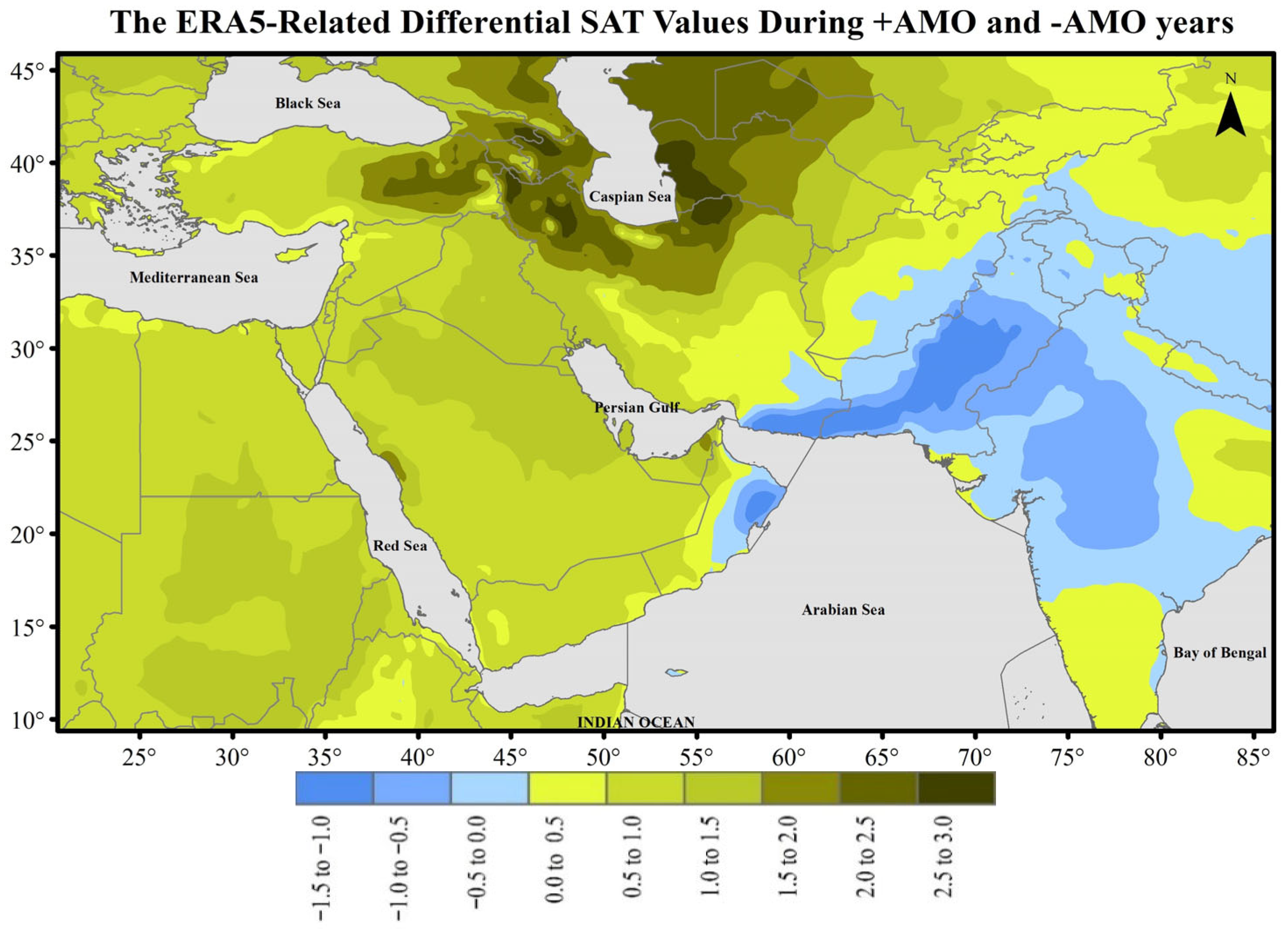
To evaluate the effects of the +AMO or −AMO on SAT variability, we calculated the differences in the mean SAT data between the two phases, defined by the formula (Diff = SAT_+AMO − SAT_−AMO). These differential values were obtained for all 151 stations (Table S1, column 9, and Figure 6) and all the ERA5-related 0.25° × 0.25° pixels (Figure 7). The illustrated circles, rectangles, and triangles in Figure 6 and the shadings in Figure 7 illustrate regions where the differential values are statistically greater or less than zero. The stations where the SAT_+AMO was significantly greater than or equal to (≥) SAT_−AMO are shown by the red circles. The insignificant differences between SAT_+AMO and SAT_−AMO are shown by either a black rectangle or a blue triangle, as indicated in the caption of Figure 6. The conducted Mann–Whitney test proved that, out of 151 studied stations, SAT_+AMO was significantly > (<) SAT_−AMO for 103 (11) stations, suggesting the influential role of the AMO extreme phases on the regional SAT values.

The presented differential values in Figure 6 generally vary from approximately −0.3 °C in regions such as Afghanistan, Pakistan, Oman, Sudan, and India to around +1.9 °C in some areas, including western Lebanon, a part of Georgia, northwestern and northern Iran, and central Saudi Arabia. Since SAT_+AMO was significantly greater than SAT_−AMO across most of the study area, +AMO (−AMO) has mostly induced positive (negative) SAT trends. While the +AMO generally harmonized with the positive trends, the occurrence of −AMO tends to suppress sharp warming rates or induce negative trends.

In some stations, such as Muscat in Oman, Multan and Lahore in Pakistan, Wad Madani in Sudan, and Pendra Road and Mumbai Santacruz in India, the differential output varies between 0 °C and −0.5 °C, indicating that climate change is insignificant in these locations. Comparing Figure 3 and Figure 6, or Figure 4 and Figure 7, suggests that the Mann-Kendall test did not prove significant changes in the SAT time series, where the output of (SAT_+AMO − SAT_−AMO) is either negative or insignificantly positive. Therefore, we concluded that AMO conditions influence climate change over the study area.

Notably, compared to Figure 6, the areas with negative differential values appear larger and more geographically continuous in Figure 7. According to this figure, northern India, most of Pakistan and Oman, the eastern half of Afghanistan, and Iran’s southeast, where climate change is generally insignificant, are the regions where the output of (SAT_+AMO − SAT_−AMO) is the lowest. As indicated in Figure 4, climate change in these regions is either insignificant or negative. Since the ERA5-related biases ranged from approximately −10% to +70%, more thorough attention is necessary to accurately interpret this dataset-associated results.

The different significance levels in Figure 6 and various shadings in Figure 7 suggest that, besides AMO, climate change over the study area is also modulated by some other climate drivers. For example, why are trend values highly positive in the northern parts of Iran and near-zero in the southeastern corner? To find a proper answer to such questions and since the southern and eastern parts of the study area are known as the monsoon-dominated regions, we were prompted to evaluate the role of monsoon in modulating SAT variability during the +AMO and −AMO. These climate specifications included the SAT, OLR, VW, omega index, and specific humidity.

3.5. The Monsoon–AMO–SAT Interactions

3.5.1. Interactions with the OLR as a Cloudiness Proxy

We have already shown that the output of (SAT_+AMO − SAT_−AMO) is close to zero for the lowland areas and highly positive for most interior highlands. In other words, while the dominance of either the +AMO or −AMO does not significantly alter SAT variability over the landmasses along the northwest Indian Ocean coasts, a high degree of variability is observed over the elevated inland regions. To address the SAT trends’ spatial variability, this section explains the reasons behind the mostly insignificant SAT trends over the monsoon-dominated lowland areas. Following this, the causes of highly significant trends in certain interior regions are discussed.

Based on some preliminary examinations, we concluded that the interactions between the AMO extreme phases and the monsoon-related cloudiness differ between the coastal areas and the interior highlands. While the cloudiness counteracts the effects of the AMO extremes on the SAT variability in lowland areas, it can amplify such effects over the interior regions. The following section explores this hypothesis in greater detail.

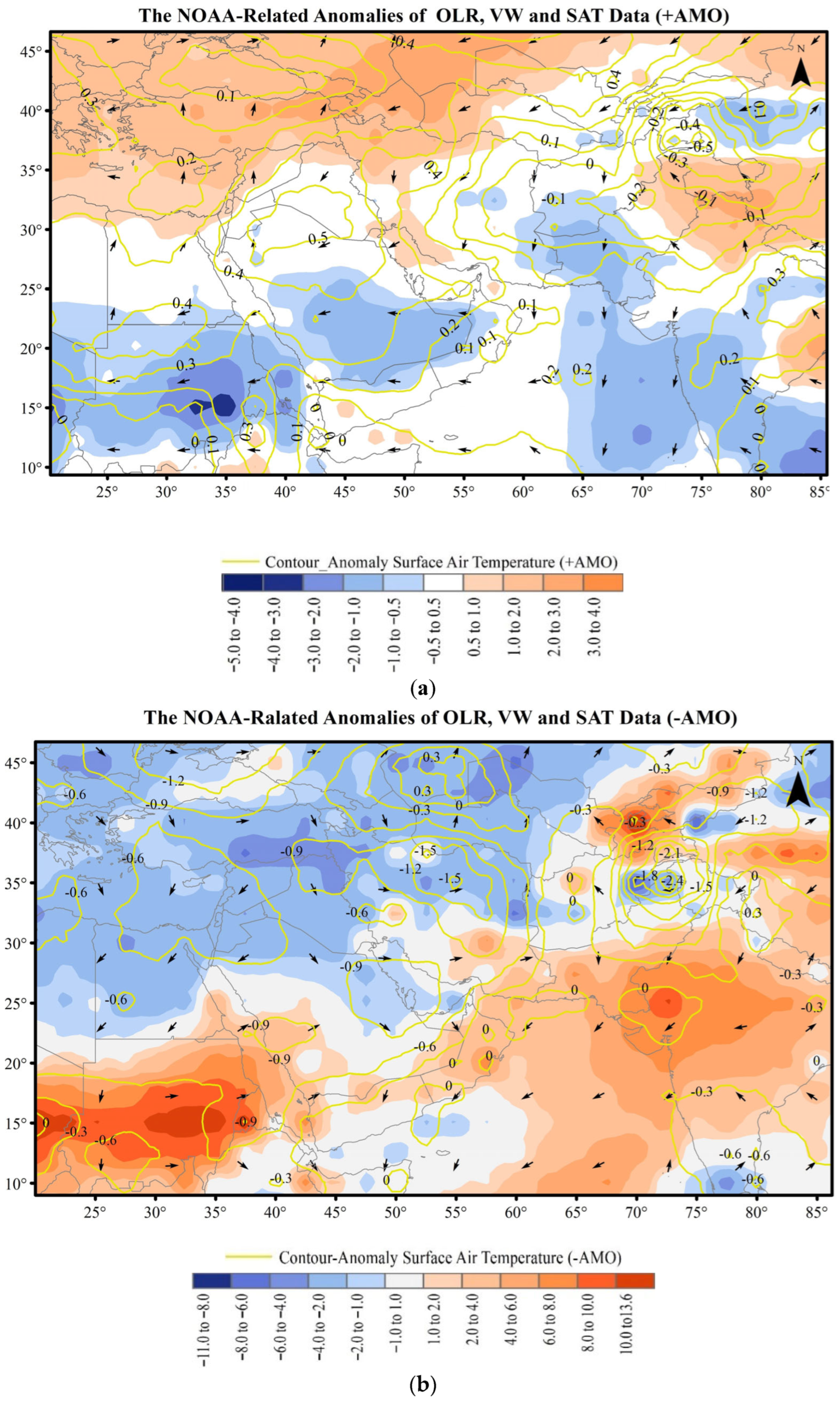
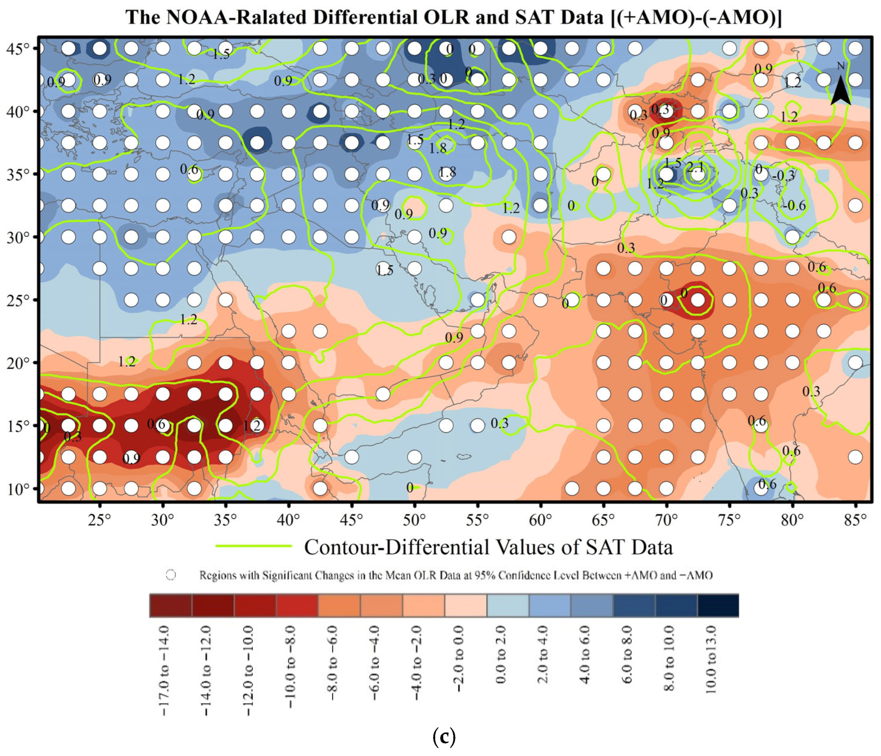
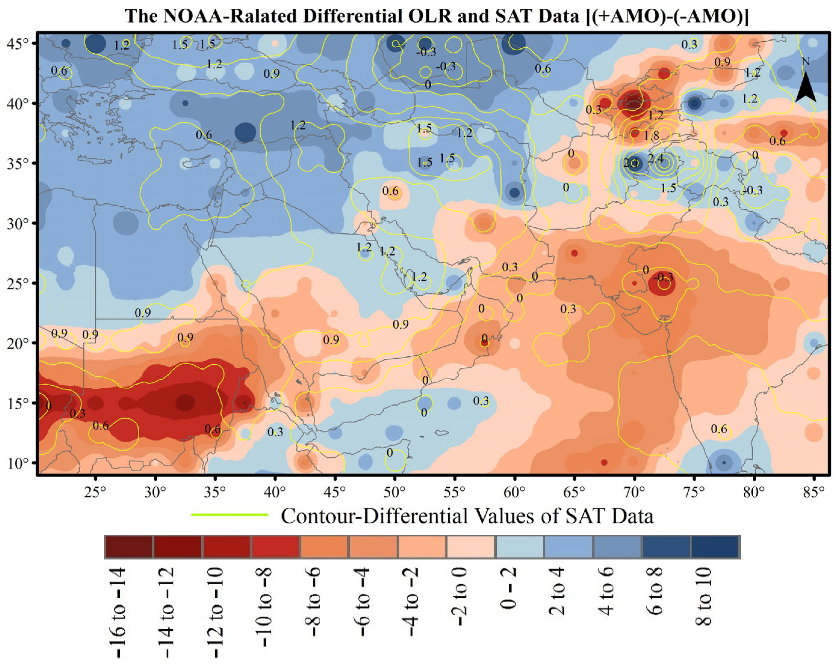
Figure 8a,b compare the anomalies of NOAA-based SAT, OLR, and the 700 hPa VW between the +AMO and −AMO years. While shading indicates the OLR anomalies, the arrows or contour lines depict the anomalies of the VW or SAT data, respectively. Notably, several studies have reported a quasi-linear relationship between SAT and OLR, emphasizing the influential role of OLR in the Earth’s climate systems [101,102]. Based on our interpretation, intensified positive OLR anomalies correspond to the periods when the anomalies of SAT or cloudiness are positive or negative, respectively. In contrast, negative OLR anomalies are typically associated with an increase in cloud cover and negative SAT anomalies [103]. While Figure 8a,b illustrate anomaly values, Figure 8c shows the differences in the mean OLR and SAT values between the +AMO and −AMO years. The contour lines in this figure, representing the output of (SAT_+AMO − SAT_−AMO), resemble those seen in Figure 6 and Figure 7, except that Figure 8c is generated according to the NOAA datasets.

Based on the blue-shaded areas of Figure 8a, the dominance of +AMO increases cloudiness over most of India, southeast of the Middle East, and tropical East Africa, where the output of (SAT_+AMO − SAT_−AMO) was generally near zero. Conversely, regions depicted with red shading indicate areas where the dominance of +AMO increases sun shining. These areas mainly include northeastern India and neighboring regions in Nepal and western China, the eastern half of Pakistan and Afghanistan, the west of the Middle East, North Africa, southern Europe, and western Russia.

For a large part of the study area, cloudiness and SAT anomalies exhibit opposite signs between +AMO and −AMO years (Figure 8a,b). However, over the southwest Indian subcontinent and the southeast Middle East, cloudiness signs differ between these phases, but associated SAT anomalies remain near zero. This aligns with our previous Mann–Whitney test results showing no significant difference between SAT_+AMO and SAT_−AMO in these regions (Figure 7). This unique behavior can be attributed to the counteracting influences of the AMO and monsoonal cloud cover. While intensified monsoonal cloudiness during +AMO reduces the expected positive SAT anomalies, enhanced clear skies during −AMO mitigate the negative SAT anomalies. Consequently, SAT anomalies in these areas remain near zero. As indicated in Figure 8c, while differences in the mean SAT data are near zero over the monsoon-dominated areas, the associated differences are significant between the OLR_+AMO and OLR_+AMO.

Unlike the southern regions (latitudes mainly below 27° N), the higher latitudes mostly encounter an increased (decreased) cloudiness during the −AMO (+AMO) (Figure 8a,b). The +AMO-related clear skies in northern Saudi Arabia increased SAT anomalies by up to +0.5 °C (Figure 8a), while the −AMO decreased SAT anomalies by up to −2.4 °C. During −AMO years, highlands in northern Afghanistan, Pakistan, and Iran exhibit a greater tendency toward increased cloudiness and associated negative SAT anomalies (Figure 8b,c). The −AMO also strengthens easterly circulations, enhancing cloud cover between northwestern China and Iran, across Central Asia. A weaker version of this circulation and increased cloudiness is also observed during +AMO. While the +AMO-related circulation aids moisture transport into southeastern Iran, the northern half of the country benefits from this moisture transfer during −AMO. Further research is needed to identify the source regions of moisture transport to Iran and the northwestern parts of the study area during extreme AMO phases.

Coherent with the presented statistics in Figure 8b, the SAT anomaly during −AMO is around −1.5 °C, across Iran’s northern half, in the southern foothill of the Alborz Mountain. Although the output of (SAT_+AMO − SAT_−AMO) in Figure 8c is more negative over Pakistan and Afghanistan’s northern highlands, the observational and ERA5 data (Figure 6 and Figure 7) do not confirm extreme differential values. On the other hand, the observational, ERA5, and Figure 8c data suggest that, for the northern half of Iran, the output of (SAT_+AMO − SAT_−AMO) is highly significant, indicating that the dominance of the AMO extreme phases, and particularly −AMO, significantly alter cloudiness and its associated SAT anomalies. Since the AMO−monsoon interactions exert a seesaw climate pattern between the red and blue shaded areas in Figure 8a–c, the frequency of the +AMO and −AMO years during the study period influence the results of the climate change analysis.

3.5.2. Interactions with the Convective Activities and Specific Humidity

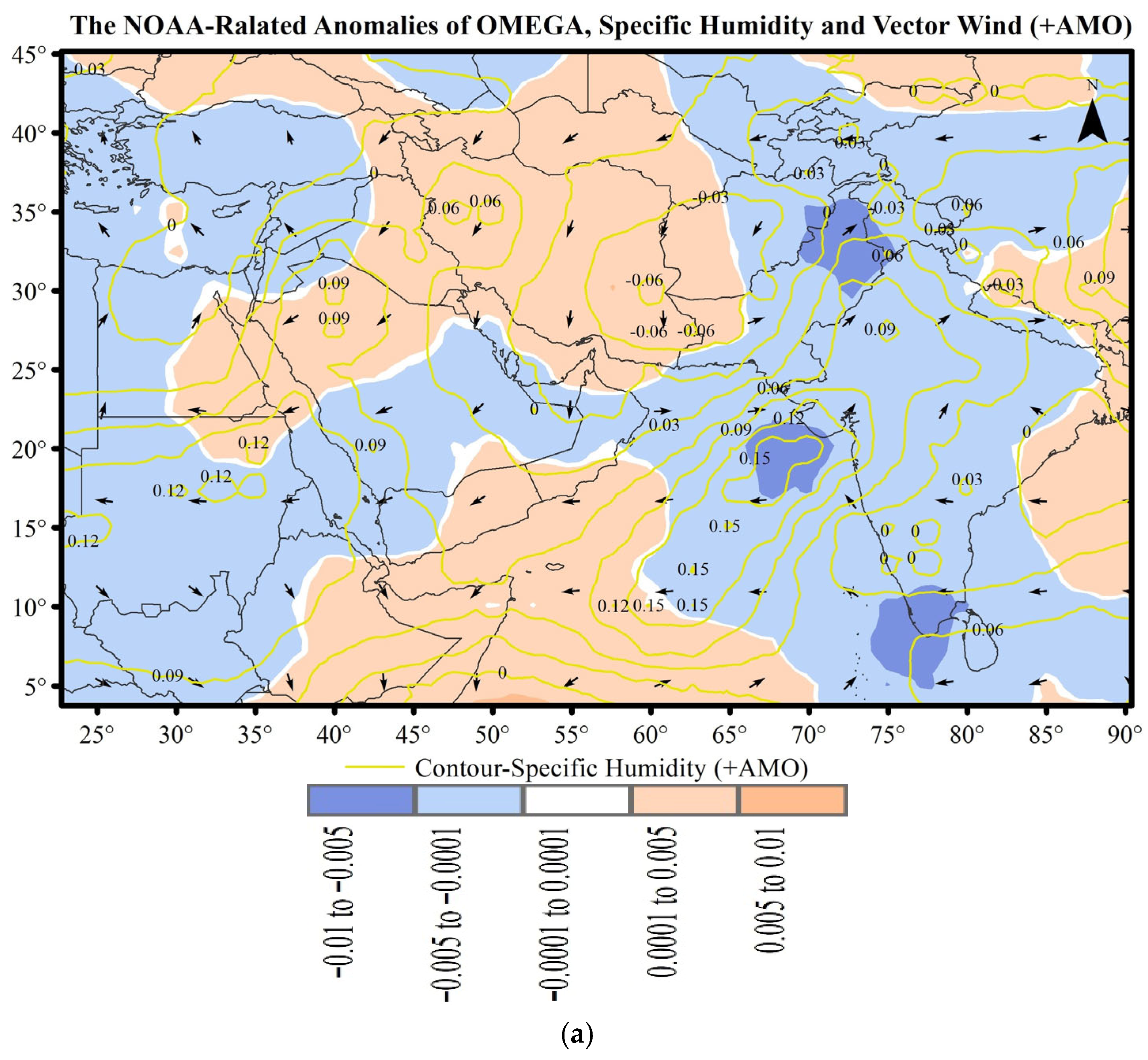
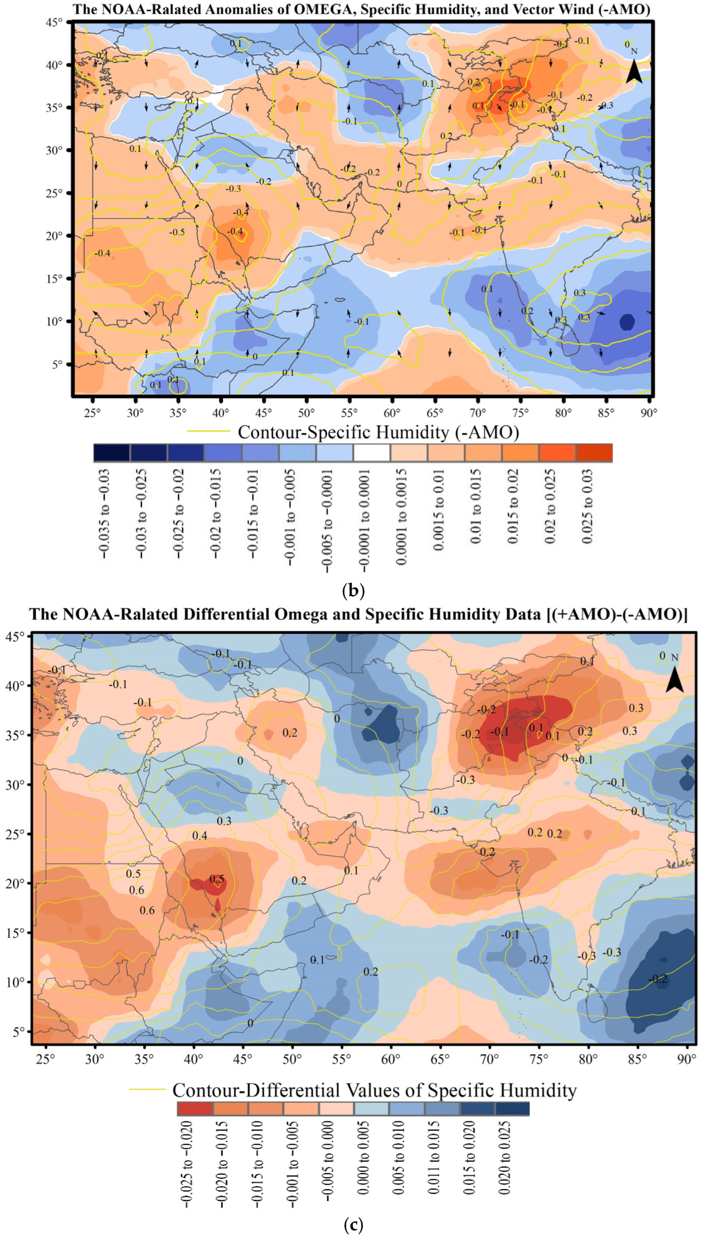
The spatial distributions of omega, vector wind, and specific humidity anomalies at 500 hPa were compared between +AMO and −AMO phases to validate the findings (Figure 9a,b). Blue (yellow) shading indicates enhanced (suppressed) convective activity, while contours (arrows) represent specific humidity (atmospheric circulation) anomalies. Figure 9c illustrates differences in mean omega and specific humidity between +AMO and −AMO, with blue (red) shading denoting regions where −AMO-related convective activity is more (less) intense than during +AMO. A Mann–Whitney test confirmed significant differences in mean omega and specific humidity between +AMO and −AMO across the study area, further supported by shifts in wind direction.

Figure 9a–c indicate increased (decreased) convective activity during +AMO (−AMO) over coastal northwest India, Pakistan, northeast Afghanistan, Iran’s southeast coasts, northern Oman, central Saudi Arabia, and Sudan and Egypt, corroborating previous findings of enhanced (suppressed) cloud cover. Specific humidity anomalies over the Arabian Sea are predominantly positive (negative) during +AMO (−AMO). Comparison of specific humidity and omega anomalies over the Arabian Sea and Bay of Bengal (Figure 9a,b) suggests that +AMO-related monsoonal activity is generally centered over the Arabian Sea, while −AMO activity is primarily located over the eastern Bay of Bengal.

3.5.3. Interaction with the Atmospheric Circulations

Figure 8a,b indicate that the 700 hPa airflow anomalies over eastern Sudan, the Arabian Peninsula, Iran, and most of India generally exhibit opposite directions between the +AMO and −AMO phases. The wind anomalies are generally westward during +AMO (Figure 8a) and shift eastward during −AMO (Figure 8b). Additionally, Figure 8a, b show easterly circulation from west China toward Afghanistan, Pakistan, and Iran during both AMO phases. The +AMO-related easterlies shift southward, potentially increasing cloud cover in southern Pakistan and southeastern Iran. Conversely, the −AMO-associated circulation increases cloudiness over northeastern Iran. Thus, in contrast to the southeastern Middle East, −AMO dominance causes cloudiness and associated coldness in most of northern Iran (Figure 8b). This wind direction opposition between +AMO and −AMO also occurs at 500 hPa (Figure 9a,b). For example, during +AMO, atmospheric circulation transports moisture from the Persian Gulf and Gulf of Oman into the central Arabian Peninsula (Figure 8a and Figure 9a), a pattern not evident during −AMO (Figure 8b and Figure 9b). Furthermore, Figure 8b and Figure 9b suggest that the eastward moisture transport from west China into Iran at 700 hPa is primarily a near-surface phenomenon, ceasing in the mid-atmosphere. Considering moisture-bearing winds, heavy rainfall is more likely to occur in north-central Iran during −AMO years and in southeastern parts of the country during +AMO years.

3.6. Threshold Sensitivity Effects

Threshold selection is crucial for defining +AMO and −AMO years. For instance, changing the thresholds from ±0.15 to ±0.2 increased +AMO-associated years to 21 while maintaining 12 −AMO years, potentially skewing results. To address this sensitivity, recalculations using ±0.2 thresholds yielded generally similar results to those using ±0.15. Figure 10, is a re-generated version of Figure 8c with the modified thresholds. Figure 11 illustrates the difference between Figure 8c and Figure 10 (Figure 11 = Figure 8c − Figure 10). While OLR (SAT)-related differences varying from −1 and 1 Watt/m² (near zero) in monsoon-dominated areas, the fluctuations are higher, from −4 to +3 Watt/m² (0.4 to −0.6 °C), for the other parts of the study area. Mann-Whitney tests found no significant difference in OLR or SAT data between Figure 8c and Figure 10. Thus, in monsoon-dominated regions, cloudiness variations during +AMO and −AMO periods counteract SAT variability, regardless of the selected threshold. However, this cloudiness may amplify SAT differences in other regions.

4. Conclusions

Our preliminary investigation indicated that the magnitude and algebraic signs of summertime SAT trends over the Middle East are site-specific and vary from one place to another. Evidence suggests that considering the interconnections between climate change in the Middle East and the Indian Subcontinent may explain some of site-specific properties. Also, some findings inferred that the differences in the trends resulted from the interactions between a few teleconnections. To avoid any speculation and after some trial and error, we analyzed climate change over the Middle East and Indian subcontinent using observational and fine-resolution ERA5 SAT data from 1961 to 2020. Subsequently, we evaluated the impacts of extreme phases of the Atlantic Meridional Oscillation (+AMO and −AMO) on these changes. To justify the site-specific responses of the AMO-SAT relationships, we used the NOAA-based datasets to examine the combined effects of the AMO and the monsoon-related activities on SAT variability. In particular, we evaluated how the monsoon-associated cloudiness and atmospheric flows modulate the impacts of the AMO extreme phases on climate change. Quantifying bias in the gridded data, assessing the elevation-bias relationships, and evaluating the adverse effects of bias on climate change analysis were the other goals of the study. The novelty of such analysis led us to conclude that the interactions between SAT, AMO, and monsoonal activities are essential in the comprehensive assessment of climate change in these regions.

Among 151 ground-based stations spread over various parts of the study area, the magnitudes of SAT data over the period 1961–2020 varied from 16 °C to 36 °C. Meanwhile, the ERA5 data fluctuated between 18 °C and 42 °C, suggesting the model’s tendency to overestimate SAT values. Regardless of using observational or gridded datasets, the Mann-Kendall test showed a significant increasing trend in SAT data of the interior highlands and a decreasing or insignificant trend in the coastal or lowland areas. These low-lying areas mainly include southern Pakistan, northern India, the southeastern coasts of Iran, and the coastal parts of Oman, Yemen, Eritrea, South Sudan, and Ethiopia. Notably, ERA5 showed 5% to 26% underestimations across these low-land regions, where trends in the SAT data were insignificant. On the other hand, overestimations of 10% to 70% were mainly detected over the high-elevation parts of the study area, where climate change was mostly positive and significant. We developed a correlation model between elevation and the ERA5-related bias, indicating that bias significantly increases with elevation.

To clarify the role of external forcing on climate change, the magnitudes of SAT_+AMO and SAT_−AMO were compared. According to the provided results, while +AMO (−AMO) induces positive (negative) trends, the forcing effects of +AMO are more than the −AMO impacts. Due to such forcing effects, the outputs of (SAT_+AMO − SAT_−AMO) are mostly positive. This output has reached about +1.8 °C in some areas, including the Caucasus region, northwestern and northern Iran, western Lebanon, a part of Georgia, and central parts of Saudi Arabia. On the other hand, this differential vale was slightly negative or insignificantly positive for some parts of Iran, Afghanistan, Pakistan, Oman, Sudan, and India. To justify such differences, the combined forcing effects of the AMO and monsoonal activities were examined. In this examination, the magnitudes of several atmospheric components comprising SAT, the monsoon-associated cloudiness, omega, specific humidity, and vector wind at the 700 and 500 hPa levels were compared between the +AMO and −AMO years.

Based on our findings, for the low-land areas in the west Indian subcontinent and the southeastern Middle East, mostly between 10° and 25° N and 20° to 85° E, the anomalies of cloud cover are positive (negative) during +AMO (−AMO). For this particular area, cloud cover induces + (−) SAT anomalies during −AMO (+AMO). Therefore, the combined impacts of the AMO and monsoon-related cloud cover counterbalance SAT variability and climate change over these specific low-land areas. While the enhanced monsoon-associated cloudiness suppresses the +AMO-caused warming rates, the (−AMO)-related coldness is compensated by further clear sky. In contrast to the mentioned lowland areas, for the northern and western parts of the study area, the regions between 25° and 50° N and 10° to 60° E, the anomalies of the +AMO (−AMO)-related cloud cover are mainly negative (positive). Our results indicated that the Arabian Sea (Bengal Gulf) are the main center of action of convective activities during the +AMO (−AMO). Moreover, the conducted sensitivity test indicated that findings of this study are not statistically sensitive to the selected thresholds for categorizing +AMO and −AMO.

It is worth noting that while the +AMO-related wind anomalies at the 700 hPa level are generally toward the core centers of the African monsoon, these anomalies tend to be westerly or southwesterly during −AMO. Moreover, we detected an easterly circulation transferring moisture from west China toward the west (Afghanistan, Pakistan, and Iran) during both +AMO and −AMO. While the +AMO-related circulation improves cloudiness over Iran’s southeast, the (−AMO)-associated circulation intensifies cloud cover over the country’s northeast and central north regions. Consequently, the likelihood of heavy torrential rainfall in the northern half and southwestern (southeastern) parts of Iran is more probable during the −AMO (+AMO) events.

5. Highlights and Recommended Future Research

This research provides findings that enable scientific communities to develop effective strategies for mitigating global warming’s adverse effects. Specifically, it demonstrates the interconnectedness of climate change in the Indian subcontinent and the Middle East, potentially fostering regional cooperation in mitigating climate change impacts. The results, which reveal the impacts of the Atlantic Multidecadal Oscillation (AMO) on surface air temperature (SAT) variability, help decision-makers to make more reliable predictions of future climate based on projected AMO. The proven interactions between AMO and monsoon improve the prediction of key meteorological elements on seasonal to sub-seasonal scales. Finally, the introduced bias-elevation relationship assists global and regional model developers in reducing model bias. Understanding these biases is essential for the accuracy of climate projections, tailoring regional strategies, enhancing model calibration, assisting informed decision-making, and determining future research directions.

By expanding these findings, policymakers can enhance community resilience by aligning their planning processes within agriculture and water management and also guard against health risks associated with heat stress in the face of climate variability.

While this study illuminates spatial variability in SAT trends, further research is recommended to address remaining questions. Future studies should incorporate more ground-based station data, especially from highland areas; assess SAT–AMO-monsoon relationships at finer geographic scales; use high-resolution gridded data for SAT, OLR, omega, and humidity; and apply these research findings to mitigate the adverse effects of global warming. Additionally, researchers are recommended to examine the mechanism of the teleconnection between AMO and the monsoon in more detail.

References

1. Mandel, A.; Tiggeloven, T.; Lincke, D.; Koks, E.; Ward, P.; Hinkel, J. Risks on global financial stability induced by climate change: The case of flood risks. Clim. Change 2021, 166, 4. [Google Scholar] [CrossRef]
2. Upadhyay, R.K. Markers for global climate change and its impact on social, biological and ecological systems: A review. Am. J. Clim. Change 2020, 9, 159. [Google Scholar] [CrossRef]
3. Giorgi, F.; Lionello, P. Climate change projections for the Mediterranean region. Glob. Planet. Change 2008, 63, 90–104. [Google Scholar] [CrossRef]
4. Waha, K.; Krummenauer, L.; Adams, S.; Aich, V.; Baarsch, F.; Coumou, D.; Schleussner, C.F. Climate change impacts in the Middle East and Northern Africa (MENA) region and their implications for vulnerable population groups. Reg. Environ. Change 2017, 17, 1623–1638. [Google Scholar] [CrossRef]
5. Gao, Y.; Jia, J.; Lu, Y.; Yang, T.; Lyu, S.; Shi, K.; Yu, G. Determining dominating control mechanisms of inland water carbon cycling processes and associated gross primary productivity on regional and global scales. Earth-Sci. Rev. 2021, 213, 103497. [Google Scholar] [CrossRef]
6. Lu, J.; Zhou, K.; Yang, M.; Zhang, P.; Shao, L.; Hilton, J. Records of organic carbon isotopic composition (δ13Corg) and volcanism linked to changes in atmospheric pCO2 and climate during the Late Paleozoic Icehouse. Glob. Planet. Change 2021, 207, 103654. [Google Scholar] [CrossRef]
7. Fujimori, S.; Hasegawa, T.; Krey, V.; Riahi, K.; Bertram, C.; Bodirsky, B.L.; van Vuuren, D. A multi-model assessment of food security implications of climate change mitigation. Nat. Sustain. 2019, 2, 386–396. [Google Scholar] [CrossRef]
8. Tai, A.P.; Martin, M.V.; Heald, C.L. Threat to future global food security from climate change and ozone air pollution. Nat. Clim. Change 2014, 4, 817–821. [Google Scholar] [CrossRef]
9. Nazemosadat, M.J.; Shafiei, R.; Ghaedamini, H.; Najjari, M.; Nazemosadat-Arsanjani, Z.; Hatam, G. Spatio-temporal variability of malaria infection in Chahbahar County, Iran: Association with the ENSO and rainfall variability. Environ. Sci. Pollut. Res. 2022, 29, 41757–41775. [Google Scholar] [CrossRef] [PubMed]
10. Waits, A.; Emelyanova, A.; Oksanen, A.; Abass, K.; Rautio, A. Human infectious diseases and the changing climate in the Arctic. Environ. Int. 2018, 121, 703–713. [Google Scholar] [CrossRef] [PubMed]
11. Cramer, W.; Guiot, J.; Fader, M.; Garrabou, J.; Gattuso, J.P.; Iglesias, A.; Xoplaki, E. Climate change and interconnected risks to sustainable development in the Mediterranean. Nat. Clim. Change 2018, 8, 972–980. [Google Scholar] [CrossRef]
12. Dottori, F.; Szewczyk, W.; Ciscar, J.C.; Zhao, F.; Alfieri, L.; Hirabayashi, Y.; Feyen, L. Increased human and economic losses from river flooding with anthropogenic warming. Nat. Clim. Change 2018, 8, 781–786. [Google Scholar] [CrossRef]
13. Lelieveld, J.; Hadjinicolaou, P.; Kostopoulou, E.; Chenoweth, J.; El Maayar, M.; Giannakopoulos, C.E.; Xoplaki, E. Climate change and impacts in the Eastern Mediterranean and the Middle East. Clim. Change 2012, 114, 667–687. [Google Scholar] [CrossRef]
14. Smith, K.R.; Chafe, Z.; Woodward, A.; Campbell-Lendrum, D.; Chadee, D.D.; Honda, Y.; Haines, A. Human health: Impacts, adaptation, and co-benefits. In Climate Change 2014 Impacts, Adaptation and Vulnerability: Part A: Global and Sectoral Aspects; Cambridge University Press: Cambridge, UK; Intergovernmental Panel on Climate Change (IPCC): Geneva, Switzerland, 2015; pp. 709–754. [Google Scholar]
15. Watts, M.J.; Monteys, V.S.I.; Mortyn, P.G.; Kotsila, P. The rise of West Nile Virus in Southern and Southeastern Europe: A spatial–temporal analysis investigating the combined effects of climate, land use and economic changes. One Health 2021, 13, 100315. [Google Scholar] [CrossRef]
16. Anchukaitis, K.J.; Wilson, R.; Briffa, K.R.; Büntgen, U.; Cook, E.R.; D’Arrigo, R.; Zorita, E. Last millennium Northern Hemisphere summer temperatures from tree rings: Part II, spatially resolved reconstructions. Quat. Sci. Rev. 2017, 163, 1–22. [Google Scholar] [CrossRef]
17. Menne, M.J.; Williams, C.N.; Gleason, B.E.; Rennie, J.J.; Lawrimore, J.H. The global historical climatology network monthly temperature dataset, version 4. J. Clim. 2018, 31, 9835–9854. [Google Scholar] [CrossRef]
18. Milly, P.C.; Betancourt, J.; Falkenmark, M.; Hirsch, R.M.; Kundzewicz, Z.W.; Lettenmaier, D.P.; Stouffer, R.J. Stationarity is dead: Whither water management? Science 2008, 319, 573–574. [Google Scholar] [CrossRef] [PubMed]
19. Osborn, T.J.; Jones, P.D.; Lister, D.H.; Morice, C.P.; Simpson, I.R.; Winn, J.P.; Harris, I.C. Land surface air temperature variations across the globe updated to 2019: The CRUTEM5 data set. J. Geophys. Res. Atmos. 2021, 126, e2019JD032352. [Google Scholar] [CrossRef]
20. Coumou, D.; Robinson, A.; Rahmstorf, S. Global increase in record-breaking monthly-mean temperatures. Clim. Change 2013, 118, 771–782. [Google Scholar] [CrossRef]
21. Paz, S.; Majeed, A.; Christophides, G.K. Climate change impacts on infectious diseases in the Eastern Mediterranean and the Middle East (EMME)-risks and recommendations. Clim. Change 2021, 169, 40. [Google Scholar] [CrossRef] [PubMed]
22. Diffenbaugh, N.S.; Giorgi, F. Climate change hotspots in the CMIP5 global climate model ensemble. Clim. Change 2012, 114, 813–822. [Google Scholar] [CrossRef]
23. Zittis, G.; Hadjinicolaou, P.; Klangidou, M.; Proestos, Y.; Lelieveld, J. A multi-model, multi-scenario, and multi-domain analysis of regional climate projections for the Mediterranean. Reg. Environ. Change 2019, 19, 2621–2635. [Google Scholar] [CrossRef]
24. Soltani, M.; Laux, P.; Kunstmann, H.; Stan, K.; Sohrabi, M.M.; Molanejad, M.; Martin, M.V. Assessment of climate variations in temperature and precipitation extreme events over Iran. Theor. Appl. Climatol. 2016, 126, 775–795. [Google Scholar] [CrossRef]
25. Jaswal, A.K.; Padmakumari, B.; Kumar, N.; Kore, P.A. Increasing trend in temperature and moisture induced heat index and its effect on human health in climate change scenario over the Indian sub-continent. J. Clim. Change 2017, 3, 11–25. [Google Scholar] [CrossRef]
26. Pai, D.S.; NAIR, S.; Ramanathan, A.N. Long term climatology and trends of heat waves over India during the recent 50 years (1961–2010). Mausam 2013, 64, 585–604. [Google Scholar] [CrossRef]
27. Rohini, P.; Rajeevan, M.; Srivastava, A.K. On the variability and increasing trends of heat waves over India. Sci. Rep. 2016, 6, 26153. [Google Scholar] [CrossRef]
28. Nayak, S.; Mandal, M.; Maity, S. Performance evaluation of RegCM4 in simulating temperature and precipitation climatology over India. Theor. Appl. Climatol. 2019, 137, 1059–1075. [Google Scholar] [CrossRef]
29. Koster, R.D.; Suarez, M.J. Impact of land surface initialization on seasonal precipitation and temperature prediction. J. Hydrometeorol. 2003, 4, 408–423. [Google Scholar] [CrossRef]
30. Alizadeh, O. A review of the El Niño-Southern Oscillation in future. Earth-Sci. Rev. 2022, 235, 104246. [Google Scholar] [CrossRef]
31. Nazemosadat, M.J.; Shahgholian, K.; Ghaedamini, H. The wet and dry spells within the MJO-phase 8 and the role of ENSO and IOD on the modulation of these spells: A regional to continental-scales analysis. Atmos. Res. 2023, 285, 106631. [Google Scholar] [CrossRef]
32. Yang, S.; Li, Z.; Yu, J.Y.; Hu, X.; Dong, W.; He, S. El Niño–Southern Oscillation and its impact in the changing climate. Natl. Sci. Rev. 2018, 5, 840–857. [Google Scholar] [CrossRef]
33. Hurrell, J.W.; Deser, C. North Atlantic climate variability: The role of the North Atlantic Oscillation. J. Mar. Syst. 2010, 79, 231–244. [Google Scholar] [CrossRef]
34. Roy, S.S. The role of the North Atlantic Oscillation in shaping regional-scale peak seasonal precipitation across the Indian subcontinent. Earth Interact. 2011, 15, 1–13. [Google Scholar] [CrossRef]
35. Donat, M.G.; Peterson, T.C.; Brunet, M.; King, A.D.; Almazroui, M.; Kolli, R.K.; Al Shekaili, M.N. Changes in extreme temperature and precipitation in the Arab region: Long-term trends and variability related to ENSO and NAO. Int. J. Climatol. 2014, 34, 581–592. [Google Scholar] [CrossRef]
36. Nazemosadat, M.J.; Shahgholian, K. Heavy precipitation in the southwest of Iran: Association with the Madden–Julian Oscillation and synoptic scale analysis. Clim. Dyn. 2017, 49, 3091–3109. [Google Scholar] [CrossRef]
37. Cullen, H.M.; Kaplan, A.; Arkin, P.A.; Demenocal, P.B. Impact of the North Atlantic Oscillation on Middle Eastern climate and streamflow. Clim. Change 2002, 55, 315–338. [Google Scholar]
38. Lu, R.; Dong, B.; Ding, H. Impact of the Atlantic Multidecadal Oscillation on the Asian summer monsoon. Geophys. Res. Lett. 2006, 33. [Google Scholar] [CrossRef]
39. Atlantic and Oceanographic and Meteorological Laboratory. Available online: https://www.aoml.noaa.gov/ (accessed on 5 September 2025).
40. B Squared, A.P.; Mudgal, A. Impact of the Atlantic Multidecadal Oscillation on surface air temperature in the United States. Atmos. Sci. Lett. 2020, 21, e961. [Google Scholar]
41. Czaja, A.; Frankignoul, C. Impact of the North Atlantic Oscillation on the European climate. Geophys. Res. Lett. 2002, 29, 1–4. [Google Scholar]
42. Masato, G.; Woollings, T.; Hoskins, B.J. Structure and impact of atmospheric blocking over the Euro-Atlantic region in present-day and future simulations. Geophys. Res. Lett. 2014, 41, 1051–1058. [Google Scholar] [CrossRef]
43. Sutton, R.T.; Hodson, D.L. Atlantic Ocean forcing of North American and European summer climate. Science 2005, 309, 115–118. [Google Scholar] [CrossRef]
44. Krishnamurthy, L.; Krishnamurthy, V. Teleconnections of Indian monsoon rainfall with AMO and Atlantic tripole. Clim. Dyn. 2016, 46, 2269–2285. [Google Scholar] [CrossRef]
45. Kumar, K.N.; Rajeevan, M.; Pai, D.S.; Srivastava, A.K.; Preethi, B. On the observed variability of monsoon droughts over India. Weather Clim. Extrem. 2013, 1, 42–50. [Google Scholar] [CrossRef]
46. Wang, C.; Lee, S.K. Atlantic warm pool, Caribbean low-level jet, and their potential impact on Atlantic hurricanes. Geophys. Res. Lett. 2007, 34. [Google Scholar] [CrossRef]
47. Ratnam, J.V.; Behera, S.K.; Ratna, S.B.; Rajeevan, M.; Yamagata, T. Anatomy of Indian heatwaves. Sci. Rep. 2016, 6, 24395. [Google Scholar] [CrossRef] [PubMed]
48. Sahu, N.; Saini, A.; Behera, S.; Sayama, T.; Nayak, S.; Sahu, L.; Duan, W.; Avtar, R.; Yamada, M.; Singh, R.B.; et al. Impact of Indo-Pacific Climate Variability on Rice Productivity in Bihar, India. Sustainability 2020, 12, 7023. [Google Scholar] [CrossRef]
49. DelSole, T.; Tippett, M.K.; Shukla, J. A significant component of unforced multidecadal variability in the recent acceleration of global warming. J. Clim. 2011, 24, 909–926. [Google Scholar] [CrossRef]
50. Zhang, H.; Wu, L. Predicting North Atlantic sea surface temperature variability on the basis of the first-mode baroclinic Rossby wave model. J. Geophys. Res. Oceans 2010, 115. [Google Scholar] [CrossRef]
51. McPhaden, M.J.; Santoso, A.; Cai, W. Introduction to El Niño Southern Oscillation in a changing climate. In El Niño Southern Oscillation in a Changing Climate; Springer: Berlin/Heidelberg, Germany, 2020; pp. 1–19. [Google Scholar] [CrossRef]
52. Park, J.H.; An, S.I.; Yeh, S.W.; Schneider, N. Quantitative assessment of the climate components driving the pacific decadal oscillation in climate models. Theor. Appl. Climatol. 2013, 112, 431–445. [Google Scholar] [CrossRef]
53. Wu, L.; Wang, C.; Wang, B. Westward shift of western North Pacific tropical cyclogenesis. Geophys. Res. Lett. 2015, 42, 1537–1542. [Google Scholar] [CrossRef]
54. Yang, Y.; Gan, T.Y.; Tan, X. Recent changing characteristics of dry and wet spells in Canada. Clim. Change 2021, 165, 42. [Google Scholar] [CrossRef]
55. Kucharski, F.; Ikram, F.; Molteni, F.; Farneti, R.; Kang, I.S.; No, H.H.; Mogensen, K. Atlantic forcing of Pacific decadal variability. Clim. Dyn. 2016, 46, 2337–2351. [Google Scholar] [CrossRef]
56. Black, E. The relationship between Indian Ocean sea–surface temperature and East African rainfall. Philos. Trans. R. Soc. A Math. Phys. Eng. Sci. 2005, 363, 43–47. [Google Scholar] [CrossRef]
57. Lolis, C.J.; Bartzokas, A.; Metaxas, D.A. Spatial covariability of the climatic parameters in the Greek area. Int. J. Climatol. A J. R. Meteorol. Soc. 1999, 19, 185–196. [Google Scholar] [CrossRef]
58. Roxy, M.K.; Chaithra, S.T. Impacts of Climate Change on the Indian Summer Monsoon; Ministry of Environment, Forest and Climate Change (MoEF&CC), Government of India: New Delhi, India, 2018. [Google Scholar]
59. Menon, A.; Levermann, A.; Schewe, J.; Lehmann, J.; Frieler, K. Consistent increase in Indian monsoon rainfall and its variability across CMIP-5 models. Earth Syst. Dyn. 2013, 4, 287–300. [Google Scholar] [CrossRef]
60. Safdar, F.; Khokhar, M.F.; Arshad, M.; Adil, I.H. Climate change indicators and spatiotemporal shift in monsoon patterns in Pakistan. Adv. Meteorol. 2019, 2019, 8281201. [Google Scholar] [CrossRef]
61. Samuelson, H.; Gaches, L. National environmental satellite, data, and information service: Providing global observations to understand earth science systems. Mar. Technol. Soc. J. 2015, 49, 23–36. [Google Scholar] [CrossRef]
62. Geen, R.; Bordoni, S.; Battisti, D.S.; Hui, K. Monsoons, ITCZs, and the concept of the global monsoon. Rev. Geophys. 2020, 58, e2020RG000700. [Google Scholar] [CrossRef]
63. Wang, B.; Liu, J.; Kim, H.J.; Webster, P.J.; Yim, S.Y. Recent change of the global monsoon precipitation (1979–2008). Clim. Dyn. 2012, 39, 1123–1135. [Google Scholar] [CrossRef]
64. Azizi, Q.; Roshani, M. The analysis of climate changes in southern shore of Caspian sea by Mann-Kendall. J. Geogr. Res. 2008, 64, 13–28. [Google Scholar]
65. Fallah-Ghalhari, G.; Shakeri, F.; Dadashi-Roudbari, A. Impacts of climate changes on the maximum and minimum temperature in Iran. Theor. Appl. Climatol. 2019, 138, 1539–1562. [Google Scholar]
66. Nazemosadat, M.J.; Samani, N.; Barry, D.A.; Molaii Niko, M. ENSO forcing on climate change in Iran: Precipitation analysis. Iran. J. Sci. Technol. Trans. B Eng. 2006, 30, 555–565. [Google Scholar]
67. Rahimzadeh, F.; Asgari, A.; Fattahi, E. Variability of extreme temperature and precipitation in Iran during recent decades. Int. J. Climatol. A J. R. Meteorol. Soc. 2009, 29, 329–343. [Google Scholar] [CrossRef]
68. Zarenistanak, M.; Dhorde, A.G.; Kripalani, R.H. Temperature analysis over southwest Iran: Trends and projections. Theor. Appl. Climatol. 2014, 116, 103–117. [Google Scholar]
69. Almazroui, M.; Islam, M.N.; Jones, P.D.; Athar, H.; Rahman, M.A. Recent climate change in the Arabian Peninsula: Seasonal rainfall and temperature climatology of Saudi Arabia for 1979–2009. Atmos. Res. 2012, 111, 29–45. [Google Scholar]
70. Muñoz-Sabater, J.; Dutra, E.; Agustí-Panareda, A.; Albergel, C.; Arduini, G.; Balsamo, G.; Thépaut, J.N. ERA5-Land: A state-of-the-art global reanalysis dataset for land applications. Earth Syst. Sci. Data 2021, 13, 4349–4383. [Google Scholar]
71. Hersbach, H.; Bell, B.; Berrisford, P.; Hirahara, S.; Horányi, A.; Muñoz-Sabater, J.; Thépaut, J.N. The ERA5 global reanalysis. Q. J. R. Meteorol. Soc. 2020, 146, 1999–2049. [Google Scholar] [CrossRef]
72. Irwandi, H.; Rosid, M.S.; Mart, T. Effects of Climate change on temperature and precipitation in the Lake Toba region, Indonesia, based on ERA5-land data with quantile mapping bias correction. Sci. Rep. 2023, 13, 2542. [Google Scholar] [CrossRef]
73. Dullaart, J.C.; Muis, S.; Bloemendaal, N.; Aerts, J.C. Advancing global storm surge modelling using the new ERA5 climate reanalysis. Clim. Dyn. 2020, 54, 1007–1021. [Google Scholar]
74. Kyle, H.L.; Weiss, M.; Ardanuy, P. Cloud, surface temperature, and outgoing longwave radiation for the period from 1979 to 1990. J. Clim. 1995, 8, 2644–2658. [Google Scholar] [CrossRef]
75. Davies, H.C.; Hanna, E. A Review of Atmospheric Blocking: Its Definition and its Role in the Climate System. J. Clim. 2000, 13, 4124–4134. [Google Scholar]
76. Ruthford, D. The Role of Atmospheric Blocking in Extreme Weather Events in the Southern Hemisphere. Weather Clim. Extrem. 2010, 2, 25–30. [Google Scholar]
77. Taszarek, M.; Allen, J.T.; Púčik, T.; Hoogewind, K.A.; Brooks, H.E. Severe convective storms across Europe and the United States. Part II: ERA5 environments associated with lightning, large hail, severe wind, and tornadoes. J. Clim. 2020, 33, 10263–10286. [Google Scholar] [CrossRef]
78. Ansari, S.; Del Greco, S.; Kearns, E.; Brown, O.; Wilkins, S.; Ramamurthy, M.; Lakshmanan, V. Unlocking the potential of NEXRAD data through NOAA’s Big Data Partnership. Bull. Am. Meteorol. Soc. 2018, 99, 189–204. [Google Scholar] [CrossRef]
79. Gruber, A.; Krueger, A.F. The status of the NOAA outgoing longwave radiation data set. Bull. Am. Meteorol. Soc. 1984, 65, 958–962. [Google Scholar] [CrossRef]
80. National Aeronautics and Space Administration Goddard Institute for Space Studies. Available online: https://data.giss.nasa.gov/gistemp/station_data_v4_globe (accessed on 20 September 2025).
81. Spanish: Agencia Estatal de Meteorología, AEMET. Available online: https://www.tutiempo.net/clima//asia.html (accessed on 20 September 2025).
82. European Centre for Medium-Range Weather Forecasts. Available online: https://cds.climate.copernicus.eu/cdsapp#!/dataset/reanalysis-ERA5-pressure-levels-monthly-means-preliminary-back-extension?tab=form (accessed on 10 September 2025).
83. National Oceanic and Atmospheric Administration. Available online: https://psl.noaa.gov/cgi-bin/data/composites/printpage.pl (accessed on 20 September 2025).
84. Yang, J.; Chang, J.; Yao, J.; Wang, Y.; Huang, Q.; Xu, G. Impact of natural climate variability on runoff based on Monte Carlo method. J. Water Clim. Change 2019, 10, 344–359. [Google Scholar] [CrossRef]
85. Lettenmaier, D.P.; Wood, E.F.; Wallis, J.R. Hydro-climatological trends in the continental United States, 1948–1988. J. Clim. 1994, 7, 586–607. [Google Scholar] [CrossRef]
86. Mann, H.B. Nonparametric tests against trend. Econom. J. Econom. Soc. 1945, 13, 245–259. [Google Scholar] [CrossRef]
87. Helsel, D.R.; Hirsch, R.M. Statistical Methods in Water Resources; Elsevier: Amsterdam, The Netherlands, 1992; Volume 49. [Google Scholar]
88. Kendall, M.G. Rank Correlation Measures; Charles Griffin: London, UK, 1975. [Google Scholar]
89. Bera, R.; Maiti, R. An assessment of coastal vulnerability using geospatial techniques. Environ. Earth Sci. 2021, 80, 306. [Google Scholar] [CrossRef]
90. Burrough, P.A.; McDonnell, R.A.; Lloyd, C.D. Principles of Geographical Information Systems; Oxford University Press: Oxford, UK, 2015. [Google Scholar]
91. Ermida, S.L.; Trigo, I.F.; DaCamara, C.C.; Jiménez, C.; Prigent, C. Quantifying the clear-sky bias of satellite land surface temperature using microwave-based estimates. J. Geophys. Res. Atmos. 2019, 124, 844–857. [Google Scholar] [CrossRef]
92. Goovaerts, P. Geostatistics for Natural Resources Evaluation; Oxford University Press: Oxford, UK, 1997. [Google Scholar]
93. Oliver, M.A.; Webster, R. Kriging: A method of interpolation for geographical information systems. Int. J. Geogr. Inf. Syst. 1990, 4, 313–332. [Google Scholar] [CrossRef]
94. Rogers, D.J.; Sedda, L. Statistical models for spatially explicit biological data. Parasitology 2012, 139, 1852–1869. [Google Scholar] [CrossRef]
95. Zhang, K.; Oswald, E.M.; Brown, D.G.; Brines, S.J.; Gronlund, C.J.; White-Newsome, J.L.; O’Neill, M.S. Geostatistical exploration of spatial variation of summertime temperatures in the Detroit metropolitan region. Environ. Res. 2011, 111, 1046–1053. [Google Scholar] [CrossRef]
96. Zimmerman, D.; Pavlik, C.; Ruggles, A.; Armstrong, M.P. An experimental comparison of ordinary and universal kriging and inverse distance weighting. Math. Geol. 1999, 31, 375–390. [Google Scholar] [CrossRef]
97. Enfield, D.B.; Mestas-Nuñez, A.M.; Trimble, P.J. The Atlantic Multidecadal Oscillation and its relationship to rainfall and river flows in the continental United States. Geophys. Res. Lett. 2001, 28, 2077–2080. [Google Scholar] [CrossRef]
98. Knight, J.R.; Folland, C.K.; Scaife, A.A. Climate impacts of the Atlantic multidecadal oscillation. Geophys. Res. Lett. 2006, 33. [Google Scholar] [CrossRef]
99. McKnight, P.E.; Najab, J. Mann-Whitney U Test. In The Corsini Encyclopedia of Psychology; Springer: Berlin/Heidelberg, Germany, 2010. [Google Scholar] [CrossRef]
100. Nachar, N. The Mann-Whitney U: A test for assessing whether two independent samples come from the same distribution. Tutor. Quant. Methods Psychol. 2008, 4, 13–20. [Google Scholar] [CrossRef]
101. Da Silva, V.D.P.R. On climate variability in Northeast of Brazil. J. Arid Environ. 2004, 58, 575–596. [Google Scholar] [CrossRef]
102. Omidvar, K.; Khosravi, Y. The analysis of some factors of climate changes in northern shore of Persian Gulf by Mann-Kendall. J. Geogr. Environ. Plan. 2010, 38, 33–46. [Google Scholar]
103. Cai, M.; Sun, J.; Ding, F.; Kang, W.; Hu, X. The Quasi-Linear Relation between Planetary Outgoing Longwave Radiation and Surface Temperature: A Climate Footprint of Radiative and Nonradiative Processes. J. Atmos. Sci. 2023, 80, 2131–2146. [Google Scholar] [CrossRef]
Figure 1. The spatial distribution of the mean summertime (June–September) SAT data during 1961–2020 (°C). Black dots refer to the geographic locations of the meteorological stations whose data were utilized in this study.
Climate 13 00221 g001
Figure 2. Similar to Figure 1, except for the ERA5 SAT data (°C).
Climate 13 00221 g002
Figure 3. The spatial distribution of the Mann-Kendall test results, represented by the Z-statistic, when the station-based values of summertime SAT data were utilized. The dark red (blue) shadings demonstrate regions where the SAT data experienced increasing (decreasing) change at 0.01 significance level. Light red and light blue shading depict the areas where changes are significant at the 0.05 significance level. The white shading indicates areas where increases or decreases in SAT were not statistically significant.
Climate 13 00221 g003
Figure 4. The spatial distribution of the Mann-Kendall test results, represented by the Z-statistic, when the ERA5-based values of summertime SAT data were utilized. The dark red (blue) shadings demonstrate regions where the SAT data experienced increasing (decreasing) change at 0.01 significance level. Light red and light blue shading depict the areas where the changes are significant at the 0.05 significance level. The white shading indicates areas where increases or decreases in SAT were not statistically significant.
Climate 13 00221 g004
Figure 5. The shading shows the spatial distribution of bias in the ERA5-related SAT dataset in °C, as described in the Methods and Results Section. As an example, in Riyadh, Saudi Arabia, the magnitudes of the observed SAT, ERA5 SAT, and bias are 35 °C, 39.6 °C, and −4.6 °C, respectively (Table S1, and this figure). This −4.6 °C bias corresponds to a 13.1% overestimation by the model.
Climate 13 00221 g005
Figure 6. The spatial distribution of the difference between the station-based summertime SAT data during the +AMO and −AMO years, defined by the formula (Diff = SAT+AMO − SAT−AMO) in °C. Red dots (blue triangles and black rectangles) specify those stations where the differential values are statistically significant (insignificant negative and insignificant positive, respectively).
Climate 13 00221 g006
Figure 7. Similar to Figure 6 but for the ERA5-based data. The blue-shaded areas signify regions where the effects of −AMO on reducing SAT values surpass the increasing impacts of +AMO. Conversely, the yellowish shadings represent regions where the influence of +AMO on increasing SAT is greater than the decreasing effects of −AMO. Notably, the differential values are mostly negative over the monsoon-affected areas, where the Mann-Kendall test did not confirm any significant changes in SAT data.
Climate 13 00221 g007
Figure 8. (a) The spatial distribution of NOAA-based anomalies for OLR (Watt/m2), SAT (°C), and 700 hPa level vector wind (m/s) during the +AMO years (Table 1). Shading represents the anomalies of OLR, while contour lines and arrows illustrate the anomalies for SAT and vector wind, respectively. Blue indicates regions where the interactions between +AMO and the monsoon enhance cloudiness, whereas red shading denotes areas where these interactions can suppress such activities. (b) Similar to Figure 8a but for the −AMO years. Blue shading indicates regions where the interactions between −AMO and the monsoon enhance convective activities and cloudiness, while red shading denotes areas where these interactions can suppress such activities. (c) The spatial distribution of NOAA-based values representing the differences in mean for OLR (Watt/m2), SAT (°C), data between the +AMO and −AMO phases. Shading shows the differences in mean OLR values, while contour lines depict differences in SAT data. Blue shading indicates regions where +AMO cloudiness is more intense than cloudiness during −AMO years. The white circles indicate the areas where OLR+AMO significantly differs from the OLR+AMO.
Climate 13 00221 g008aClimate 13 00221 g008b
Figure 9. (a) The spatial distribution of NOAA-based anomalies for omega (hPa/s), specific humidity (g/kg), and vector wind (m/s) at 500 hPa level (m/s) for the +AMO years. (b) Similar to Figure 9a but for the −AMO years. Shading represents the omega anomalies, while contour lines or arrows refer to the anomalies for specific humidity or vector wind, respectively. (c) The spatial distribution of NOAA-based values of the differences in mean omega (hPa/s) or specific humidity (g/kg) data between the +AMO and −AMO years.
Climate 13 00221 g009aClimate 13 00221 g009b
Figure 10. Like Figure 8c, except for the ±0.2 thresholds. Shadings show the differences in means OLR values, while contour lines depict differences in SAT data. Blue shading indicates regions where +AMO cloudiness is more intense than cloudiness during −AMO years.
Climate 13 00221 g010
Figure 11. The spatial distribution of NOAA-based values of the differences between Figure 8c and Figure 10. Shadings (contour lines) show the differences in OLR (SAT) values. These differential values were not significant at 95% level.
Climate 13 00221 g011