Abstract
The hydrological response to meteorological drought is often nonlinear, due to physiographic features and human activities, necessitating methodologies that surpass simple drought indices. This study investigates whether drought propagation can be statistically modeled, identifies factors influencing the time lag between meteorological and hydrological droughts, and evaluates the most suitable temporal scales of drought indicators. Meteorological droughts were detected using Standardized Precipitation Index (SPI), while hydrological droughts were identified by the Adapted Threshold Level Method (ATLM), which balances available reservoir volume and the water demand, including withdrawals and evaporation losses. Castanhão, Banabuiú, and Orós reservoirs, in the State of Ceará, Brazil, were used to study drought events, across three aggregated time scales of 12, 24, and 36 months. The propagation time was determined using three indicators, corresponding to onset (Δb), peak (Δp), and conclusion (Δe) lags. Longer meteorological droughts were found to propagate more slowly to hydrological systems, with temporal lags following a consistent order of Δp > Δb > Δe. The combination of SPI-12 and ATLM-36 droughts provided the strongest and most consistent positive correlations (95% confidence level) between drought duration and all three lag markers. This combination offers a robust framework for modeling drought propagation dynamics and improving water resource management strategies.
1. Introduction
Population growth and the expansion of the agricultural, energy, and industrial sectors have led to increased water demand to meet human and production needs [1]. Conversely, under the influence of global climate change, drought events are becoming more frequent, intense, and prolonged [2,3].
Typically, drought develops slowly and can have severe impacts on water resources, the environment, human life, and socioeconomic activities [4]. Due to its complex nature, with multiple triggering factors across different temporal and spatial scales, there is no single comprehensive definition of drought, and various alternatives have been proposed in the scientific literature [5,6]. Van Loon et al. [7], for instance, defined droughts as an exceptional periods of water scarcity that negatively impact human activities or environmental demands. The Intergovernmental Panel on Climate Change (IPCC) defines drought as “a period of abnormally dry weather long enough to cause a serious hydrological imbalance” [8].
Generally, droughts are classified into four types: meteorological drought, hydrological drought, agricultural drought, and socioeconomic drought [6,9]. Meteorological drought is related to precipitation deficits, possibly combined with increased evapotranspiration; agricultural drought is linked to soil moisture deficits, reducing water availability for vegetation and potentially leading to crop loss; hydrological drought is associated with negative anomalies in hydrological variables—typically streamflow and groundwater storage—and can develop over seasonal or interannual periods; and socioeconomic drought occurs when water availability is insufficient to meet stakeholder needs, affecting industry, livelihoods, health, and more [10].
When drought develops, it triggers cascading effects across meteorological, hydrological, and agricultural systems, with severe consequences for water resources, the environment, human life, and socioeconomic activities [4]. Previous research has shown that meteorological drought is widely recognized as the origin of other drought types due to its earlier onset [11,12]. This transition between drought types is known as drought propagation [13]. As an essential component of the hydrological cycle, the propagation from meteorological to hydrological drought significantly impacts water resource management and remains a relevant research topic worldwide [14,15]. Luo et al. [16], for example, investigated the dynamic mechanisms of drought propagation in China, using convergent cross mapping, a strategy originally applied in ecology. Jeong et al. [17] applied a time-lagged correlation analysis to determine the propagation time from meteorological to hydrological drought in South Korea. Despite advances in understanding drought propagation, its mechanisms remain highly complex and nonlinear, shaped by interactions between regional climate, hydrological, and landscape characteristics [18].
The complexity of drought propagation is partly due to the diversity and limitations of the methods used to study it. The maximum correlation method [19,20,21,22,23] and the theory of runs [11,14,15,24] stand out as the most commonly used. In the maximum correlation method, propagation time is typically determined through correlation analysis between the time series of standardized drought indices, applicable across multiple time scales. However, since the entire time series is considered, encompassing both dry and wet periods, the emphasis is placed on the relationship between precipitation and flow rather than on the propagation of drought [10]. On the other hand, the theory of runs often involves setting a certain threshold level. When each type of drought falls below this threshold, that moment is considered the beginning of the event for that type of drought. The difference between the onset times of the two types of drought events is considered as the propagation time [25]. However, this method assumes drought propagation to be a linear process, which may not hold true in many situations [12].
Bevacqua et al. [24] observed that analyzing the correlation between drought indices alone does not fully capture the dynamics of drought propagation. Additionally, they noted significant variations in the timing of drought onset, peak, and conclusion across different cases. In light of these findings, they suggest adopting multi-indicator approaches to identify the mechanisms of drought development and propagation throughout the hydrological cycle.
Although numerous studies have focused on explaining the propagation from meteorological to hydrological drought [14,22,24,26,27,28], some gaps remain. In this work, we seek to answer the following questions: (A) Is it possible to model drought propagation statistically? (B) What factors can predict the time lag between meteorological and hydrological drought? (C) Which time scales of meteorological and hydrological drought indices are most suitable for modeling drought propagation?
This article proposes a methodology for identifying patterns and statistically modeling the propagation of meteorological droughts into hydrological droughts in reservoirs. In order to identify meteorological drought events, we employed the Standardized Precipitation Index (SPI). For assessing hydrological drought, we utilized the Adapted Threshold Level Method (ATLM). Drought events were characterized by their frequency, duration, severity, magnitude, and recovery across different time scales, with data aggregated for 12, 24, and 36 months. To determine the propagation time from meteorological drought to hydrological drought, we calculated three indicators corresponding to the time differences between the onsets, peaks, and ends of the propagated drought events.
The Threshold Level Method (TLM) emerges as a more effective approach for identifying hydrological droughts, as it incorporates land-use and water demand data, overcoming the limitations of standardized indices that focus solely on reservoir inflows [26,27]. Based on run theory [28], TLM defines drought events when streamflow or storage falls below a critical threshold [29,30]. For perennial rivers, the threshold is typically set between the 70th (Q70) and 95th (Q95) percentile flows, while intermittent rivers require lower percentiles depending on zero-flow frequency [29].
However, TLM faces challenges in semi-arid regions with ephemeral rivers, where thresholds may be zero due to prolonged no-flow conditions [31]. To address this, an adaptation by Medeiros et al. [32] was employed, defining hydrological drought when reservoir storage falls below a predefined threshold. Here, the threshold is determined by summing basin water demands and reservoir evaporation losses. TLM thus quantifies actual water deficits using raw time series rather than normalized variables [26,27], offering a more effective approach for local-scale water management [30]. Given the complexity of drought propagation and the need for context-adapted methodologies, an integrated analysis of meteorological and hydrological components is essential to understand transition mechanisms. This is particularly relevant in semi-arid basins, where interactions between climate, water demands, and basin characteristics intensify multi-year drought impacts.
2. Materials and Methods
2.1. Study Area
The study area includes the Jaguaribe and Banabuiú Valleys, located within the Jaguaribe watershed in the state of Ceará, Brazil. This watershed spans a total area of 74,000 km2, representing approximately 50% of the state’s territory. It comprises five sub-watersheds: the Upper, Middle, and Lower Jaguaribe, Banabuiú, and Salgado. The climate in this region is characterized as tropical and semi-arid, with average annual temperatures ranging from 26 to 28 °C and an average rainfall of approximately 700 mm. With pronounced seasonality, rainfall is concentrated in the first half of the year, while the second half is known as the dry season. High potential evapotranspiration rates (2100 mm), coupled with spatial and temporal variability of precipitation—a hydroclimatic trait of Ceará—result in a significant water deficit, leading to the formation of intermittent rivers [33]. These rivers typically flow during the state’s rainy season, occurring from January to April [34].
In this region, water demand is mainly met by the stored water in reservoirs. Among them, 153 reservoirs are monitored and the three major ones were selected: Banabuiú (with an accumulation capacity of 1534.00 hm3), Castanhão (with an accumulation capacity of 6700.00 hm3), and Orós (with an accumulation capacity of 1940.00 hm3). These reservoirs are located in the Banabuiú, Middle Jaguaribe, and Upper Jaguaribe sub-watersheds, respectively.
The Banabuiú and Castanhão reservoirs are located downstream within the watershed, running parallel to each other, while the Orós reservoir is situated at the outlet of the Upper Jaguaribe sub-watershed. The Orós reservoir plays a crucial role as a water source for the Middle and Lower Jaguaribe regions, ensuring the continuous flow of the Jaguaribe River until it reaches the Castanhão reservoir (Figure 1).
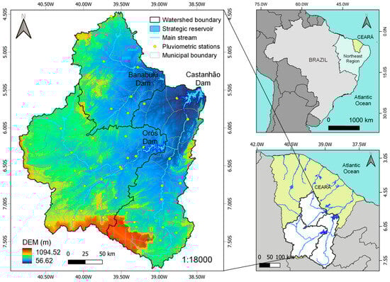
Figure 1.
Location of the watershed of the Banabuiú, Castanhão and Orós reservoirs in the State of Ceará, Brazil. The colors on the right side of the figure represent the digital elevation model (DEM).
These reservoirs were selected due to their strategic significance to the state of Ceará, as they supply water for various purposes, including drinking, agriculture, livestock, and other economic activities across multiple municipalities in the state [35].
2.2. Data Collection
The monthly precipitation data for the watershed of the studied reservoirs were sourced from FUNCEME, spanning from 1974 to 2023. Rain gauge stations with more than 30 years of data were selected and then interpolated using the Inverse Distance Weighting (IDW) method to derive the regional average monthly precipitation for each reservoir watershed.
Evaporation data covering the period from 1980 to 2010 were obtained from the climatological normals. These data corresponded to the nearest stations with available data: Jaguaruana Station (Code 82493) for the Castanhão reservoir, Iguatu Station (Code 82686) for the Orós reservoir, and Quixeramobim Station (Code 82586) for the Banabuiú reservoir. These datasets were retrieved from the National Institute of Meteorology (INMET) website. The average evaporation data from the climatological normals were measured using a Piché evaporimeter, to which a correction factor of 1.17 was applied to estimate evaporation in the reservoirs.
The historical reservoir monitoring data for the Banabuiú and Orós reservoirs were provided by FUNCEME, covering the period from 1986 and 2023. For the Castanhão reservoir, the data were available from the start of its operation in 2004 until 2023. The stored volumes were computed by monitoring the reservoir levels and using the Quota–Area–Volume (QAV) ratio of each reservoir to estimate the monthly volume based on the water level. Similarly, the evaporated volumes were estimated by multiplying the monthly evaporation rates, obtained from the climatological normals, by the surface area of the lake on the first day of each month.
Data on the demands for each reservoir were obtained from the Seminar on Negotiated Allocation of the Waters of the Jaguaribe and Banabuiú Valleys, organized by the Water Resources Management Company (COGERH) in July 2023. This seminar is an event designed to discuss and define the distribution of water among various users, ensuring democratic participation in water allocation. It determines the flows to be released for various purposes based on allocation scenarios, using the year 2022 as a reference.
2.3. Methodology
In this study, we utilized the widely recognized Standardized Precipitation Index (SPI), developed by McKee et al. [36], to determine meteorological drought. For evaluating hydrological drought, we used the Adapted Threshold Level Method (ATLM), as developed by Medeiros et al. [32].
Across all three cases, drought events were characterized by their frequency, duration, severity, magnitude, and recovery time, with data aggregated for 12, 24, and 36 months. However, due to the inherent limitations of the methodologies used, our analysis focused on comparing the periods of identified drought events to understand the occurrence of drought propagation in the study region.
2.3.1. Standardized Precipitation Index (SPI)
To analyze the meteorological drought events spanning from 1974 to 2023 in the Castanhão, Orós, and Banabuiú reservoirs, we employed the Standardized Precipitation Index (SPI). SPI is derived by fitting precipitation data to the gamma probability distribution. Subsequently, the probabilities of occurrence for each precipitation value are calculated by applying the inverse of the normal distribution, thereby identifying deviations from the average precipitation for the analyzed intervals [37,38]. A drought event commences whenever the index value turns negative and persists until it rises above zero again [36].
SPI is widely used worldwide due to its versatility in analyzing both drought and flood periods, ease of calculation, and requirement of only precipitation data. However, it is recommended to use SPI with a series of monthly values spanning at least 30 years, ideally extending to 50 or 60 years [39].
For our analysis, we used SPI-12, SPI-24, and SPI-36, representing twelve, twenty-four, and thirty-six months, respectively. These periods allow for examination of the effects of drought across different sectors and on water scarcity [40]. SPI-12 captures annual rainfall deficits and their impacts on soil moisture, crop production, and small reservoirs, being sensitive to the region’s pronounced seasonality. SPI-24 captures prolonged droughts that influence aquifers and medium-sized reservoirs, crucial for monitoring water scarcity in urban and irrigation areas. Finally, SPI-36 is associated with large reservoirs and river basins, as it identifies multi-year droughts critical for water planning and food security, as observed during extreme events (e.g., 2012–2016). These scales are widely validated in studies such as Marengo et al. [41] and Tomasella et al. [42], which highlight their effectiveness in analyzing the propagation of meteorological to hydrological droughts in Northeast Brazil. Additionally, longer time scales of SPI tend to exhibit strong correlation with hydrological drought indicators.
The same analyses were also conducted using the Standardized Precipitation Evapotranspiration Index (SPEI), which accounts for the effects of both precipitation and potential evapotranspiration, thereby providing a more comprehensive assessment of drought conditions. However, as the results obtained with SPEI were very similar to those derived from SPI, without adding substantial information to the conclusions of this study, only the SPI-based results are presented herein; the SPEI results can be found in the Supplementary Material (Figures S3–S11).
2.3.2. Adapted Threshold Level Method (ATLM)
The Threshold Level Method serves as a valuable tool for quantifying hydrological drought by assessing the water volume below a specific threshold, thereby allowing for the determination of drought characteristics such as duration, severity, and magnitude. In this study, we adapted the threshold level method originally developed by Medeiros et al. [32], which defines hydrological drought as occurring when the reservoir’s storage volume falls below a predetermined threshold.
This threshold level accounts for not only water losses due to evaporation but also losses stemming from the demands of various uses. Additionally, our study incorporated time factors (tf) of 12, 24, and 36 months, representing future periods during which the accumulated water in the reservoir at time t can meet the demands while also accounting for evaporation losses. These time periods were selected to align with the analysis of drought propagation using the SPI-12, SPI-24 and SPI-36.
Using the same time factor (tf), the threshold level (TL(tf)) was determined by summing the withdrawals needed to fulfill all the demands associated with the reservoir (Dem(tf)) and the evaporated volume (EVP(tf)), as shown in Equation (1).
The value of EVP(tf) was calculated using Equation (2), where t represents the time in months, E is the historical average of the lake’s monthly evaporation in meters per month (m.month−1), PRC is the historical average of the monthly precipitation in meters per month (m.month−1), and A is the area in square meters (m2) on the first day of each month of the reservoir watershed monitoring data series:
The hydrological variable used for calculating the water deficit is the monthly reservoir storage volume (Vol(t)), obtained from the monitoring records maintained by COGERH. Thus, the volume of water deficit (WD(tf)) was computed using Equation (3).
In the event of WD(tf) < 0, a hydrological drought occurs, which persists until the volume stored in the reservoir exceeds the threshold level considered in the analysis (WD(tf) >= 0).
2.3.3. Characterization of Droughts
Characterization of droughts was conducted for each reservoir and each index, encompassing the determination of the number of drought events, their frequency, duration, severity, intensity or magnitude, and recovery time following a drought event (both meteorological and hydrological).
Frequency was calculated by dividing the total number of months experiencing drought by the total number of months analyzed. Duration represents the time, in months, from the onset () to the conclusion () of each drought event. The severity of meteorological drought was determined by summing the SPI and the SPEI values, while the severity of hydrological drought was evaluated based on the sum of the Water Deficit values. Intensity or magnitude of the drought was determined by dividing its severity by its duration. Furthermore, drought recovery time () was determined by establishing the duration it takes for a drought event to subside after reaching its peak severity. Thus, drought recovery time was calculated by subtracting the end month () from the peak month () of the event.
2.3.4. Mutually Dependent Droughts and Minor Droughts
In this study, the definition of meteorological and hydrological wet and dry periods adheres to the theory of runs, as introduced by Yevjevich [28]. According to this theory, a series of drought events below a certain threshold level may include periods intermittent, low-magnitude wet events occurring between two consecutive drought events. In such cases, droughts are considered mutually dependent, necessitating their grouping to establish a consistent definition of drought events [43]. To achieve this grouping, we employed the Inter-Event Time Method (IT Method), introduced by Zelenhasic and Salvai [44], as depicted in Figure 2.
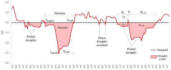
Figure 2.
Representation of the characteristics of drought events, including duration, severity, and drought recovery time (), based on the scale of the SPI. The same characterization was conducted for hydrological drought using the ATLM. For illustrative purposes, random data were used to demonstrate the pooling of mutually dependent droughts and the exclusion of minor droughts.
In this approach, two mutually dependent droughts are consolidated if the duration between them is less than a predefined number of days (tc), specifically if τi ≤ tc. The duration of a pooled drought event () is therefore defined from the first day of the first drought event () to the last day of the cluster’s last drought event (), including the excess period (τi) (Equation (4)). For this study, a tc of one month was chosen.
On the other hand, minor droughts are characterized by being short-lived and having low deficit volume. A multitude of minor droughts can distort the analysis of drought frequency over time, necessitating the exclusion of minor droughts [43]. Accordingly, all drought events lasting one month or less were excluded from the analysis.
Following the exclusion of minor droughts and the establishment of the duration of the pooled drought, the severity of the pooled drought () was determined by summing the deficit volumes from the first drought event () and the last drought event () and subtracting the excess volume of the intermediate event () (Equation (5)).
In studies addressing reservoir management, subtracting the excess volume from the total of the deficit volumes offers a more accurate depiction of reservoir withdrawal and replenishment processes [29]. This approach has been adopted by Chen et al. [45], Pandey et al. [46], Sung and Chung [47] and Tallaksen et al. [43].
2.3.5. Propagation of Droughts
The determination of the propagation time from meteorological drought to hydrological drought was obtained through the calculation of three indicators, as outlined by Bevacqua et al. [24]. The first indicator concerns the time differences between the beginnings of each meteorological drought and hydrological drought event (Δb), and the second corresponds to the time difference between the peaks of these events (Δp). The third indicator involves the time differences between the ends of the events (Δe) (Figure 3). To determine hydrological drought resulting from a meteorological drought, it was established that (i) the meteorological drought must begin before the hydrological drought, (ii) the hydrological drought must start before the meteorological drought ends, and (iii) the peak and end of the meteorological drought must occur before the peak and end of the hydrological drought.
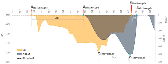
Figure 3.
Propagation of the different types of droughts using indicators that determine the time difference between the onsets (Δb), peaks (Δp), and ends (Δe) of the meteorological and hydrological droughts. Random data were used for illustrative purposes to demonstrate the calculation of the indicators under predefined conditions. and denote the beginning month, and denote the peak month, and and denote the end month of the meteorological drought (SPI) and hydrological drought (ATLM), respectively.
The total propagation time can thus be determined by averaging the time intervals between the onset, peak, and end of drought events propagated in the study area [22,48].
3. Results
The values of the SPI were determined for the annual (12 months), biennial (24 months), and triennial (36 months) time scales, spanning from 1975 to 2023. The same time scales were used to define water deficits by ATLM, where only the periods in which the indices fell below 0.0 (defined as the drought threshold) are depicted for the watersheds of the Banabuiú, Castanhão, and Orós reservoirs.
Meteorological and hydrological droughts identified from drought indices at different time scales were matched according to the previously defined criteria, allowing the identification of meteorological droughts that propagated into hydrological ones. The identified pairs of propagating droughts (from meteorological to hydrological) are presented in Table 1. It should be noted, however, that the number of droughts that met the propagation criteria (i.e., 61 droughts, Figure S1) was lower than the number of droughts initially identified (i.e., 171 droughts), considering the sum of drought cases.

Table 1.
Drought propagation across the Banabuiú, Castanhão, and Orós reservoir watersheds, indicating the average time difference (in months) between the peak (Δp), onset (Δb), and conclusion (Δe) of meteorological and hydrological drought events. The values that have the longest propagation times are highlighted in bold.
The results presented in Table 1 indicate a clear dependence of drought propagation behavior on both the temporal scale of the meteorological indicator and the hydrological aggregation period. Specifically, combinations pairing a short-term meteorological index (SPI-12) with a long hydrological integration (ATLM-36) produced the largest number of detected propagation events and the most coherent lag estimates, with a recurrent ordering of lag magnitudes (Δp > Δb > Δe) across reservoirs. These patterns suggest that short accumulation windows better capture abrupt meteorological deficits, while longer hydrological windows reflect reservoir storage inertia and cumulative catchment memory, thus improving the detectability of meteorological to hydrological propagation. Reservoir-specific differences (e.g., consistently larger Δp and Δe in Orós relative to Castanhão and Banabuiú) further indicate that storage capacity, operational rules, evaporation losses, and withdrawal regimes substantially modulate propagation speed and recovery time.
Figure 4 presents the drought propagation time (in months) between different stages of meteorological drought and the corresponding hydrological response. The variable “Propagation delta (months)” refers to the lag time between meteorological drought events (beginning, peak and end) and their observed impact on the water system. In Figure 4a, droughts events were grouped into four categories based on their duration: up to 2 years, 2 to 4 years, 4 to 6 years, and more than 6 years. Meteorological drought was taken as the reference for duration. Due to the small number of events, droughts in the three watersheds were grouped together in this analysis, regardless of the scale of the drought indices, totaling the number of events shown in Table 2. For droughts lasting up to 2 years, propagation times are relatively short (generally under 25 months), with little difference among the three reference points (drought beginning, peak, and end). This suggests that short droughts result in a quicker hydrological response. In the 2 to 4-year category, propagation times increase, especially when referenced to the drought end, indicating that hydrological recovery takes longer than the meteorological signal would suggest. There is also more variability, suggesting lower predictability. For droughts of 4 to 6 years and more than 6 years, propagation becomes slower and more prolonged, with median values between 25 and 50 months. The drought peak shows the highest propagation lags, meaning the most critical impacts on reservoir systems occur significantly after the meteorological peak. Recovery times (referenced to drought end) are generally the shortest but still show considerable delays, reflecting the sluggish replenishment of water levels even after meteorological droughts have ended.
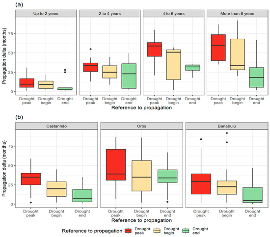
Figure 4.
Propagation delta (in months) between meteorological and hydrological droughts considering different drought reference points—peak (red), beginning (yellow), and end (green)—represented as boxplots. The whiskers cover the range from Q1–1.5 × IQR to Q3 + 1.5 × IQR: (a) Propagation delta grouped by drought duration: up to 2 years, 2–4 years, 4–6 years, and more than 6 years; (b) Propagation delta for the three major reservoirs in Ceará: Castanhão, Orós, and Banabuiú. The black dots represent the outliers.
Table 2.
Accounting for droughts grouped according to the duration of the propagation delta.
Figure 4b presents the propagation time by the three major reservoirs in Ceará, Brazil: Castanhão, Orós, and Banabuiú. In this analysis, droughts were grouped together, regardless of the scale of the drought indices, totaling 13 droughts in Castanhão, 18 droughts in Orós, and 30 droughts in Banabuiú. The median propagation time is spatially represented in Figure 5. In Castanhão, the median propagation time from the drought peak is around 35 months, indicating a delayed but steady impact. The hydrological response to the drought end is relatively quick (median under 10 months), suggesting that this reservoir system can recover more efficiently. Orós shows the longest propagation times across all reference points, especially from the drought peak. Hydrological recovery is also slower, suggesting higher vulnerability or a greater dependence on sustained rainfall for recovery. Banabuiú exhibits lower median propagation times than the other two reservoirs but with greater variability. This indicates a more sensitive and possibly reactive system, with quicker responses but less predictability.
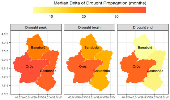
Figure 5.
Spatial representation of propagation delta (in months) between meteorological and hydrological droughts considering different drought reference points—peak, beginning, and end.
Thus, in general, it was observed that the lag between the peak of hydrological drought relative to meteorological drought is longer than the lag between their onsets, which in turn is longer than the lag between their ends—a pattern that is consistent across different reservoirs and drought durations (Figure 6). In other words, Δp > Δb > Δe. Furthermore, longer-lasting meteorological droughts tend to propagate more slowly, with greater lags between meteorological and hydrological drought markers, especially with respect to the drought peak. In other words, longer durations correspond to larger deltas (Figure 7).
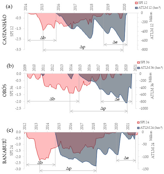
Figure 6.
Standardized Precipitation Index (SPI) and Adapted Threshold Level Method (ATLM) time series for 12-, 36-, and 24-month scales, highlighting the propagation lags between meteorological and hydrological drought events in (a) Castanhão, (b) Orós, and (c) Banabuiú.
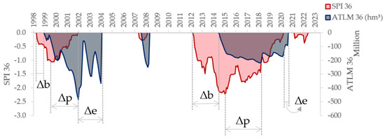
Figure 7.
Standardized Precipitation Index (SPI-36) and Adapted Threshold Level Method (ATLM-36) time series, illustrating meteorological and hydrological drought propagation events and their respective lags for the period 1998–2023.
Additionally, results indicate that the temporal lag between meteorological and hydrological droughts can be modeled as a function of drought duration (Figure 8). For this analysis, the droughts from the three watersheds were grouped together. Pearson’s correlation test was applied between the duration of the meteorological drought and the propagation lag. It was applied for different combinations of SPI and ATLM time scales and for each lag marker (Δp, Δb, and Δe). In the Pearson’s correlation test, the test statistic follows a t-distribution, which allows construction of 95% confidence intervals based on Fisher’s Z transformation and testing of the alternative hypothesis (Hₐ: ρ ≠ 0) (see Table 3).
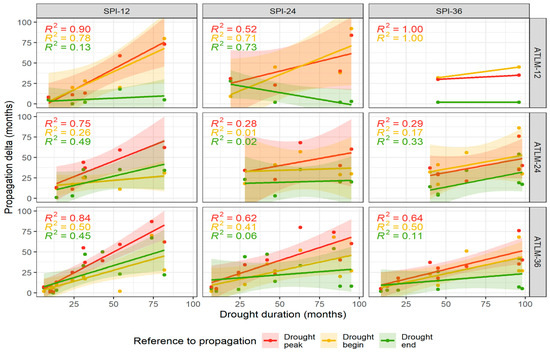
Figure 8.
Relationship between meteorological drought duration (months) and propagation lag to hydrological drought (months) for different drought indices and time scales. Columns correspond to Standardized Precipitation Index (SPI) at 12-, 24-, and 36-month scales, and rows correspond to the Adapted Threshold Level Model (ATLM) at 12-, 24-, and 36-month scales. Propagation lags are calculated with respect to three meteorological drought reference points: drought peak (red), drought beginning (yellow), and drought end (green). Solid lines represent linear fits, with shaded areas indicating 95% confidence intervals and the dots represent the propagated drought events.
Table 3.
Pearson correlation results (95% confidence level) between meteorological drought duration and temporal propagation lags (Δp, Δb, and Δe) for different combinations of SPI and ATLM accumulation periods. “Evidence” indicates statistical support for the alternative hypothesis (ρ ≠ 0) within the specified confidence interval; “No evidence” indicates the absence of a significant correlation.
Among all indicator combinations evaluated, SPI-12 for meteorological drought and ATLM-36 for hydrological drought emerged as the most suitable. This pairing was the only one to show consistent evidence of positive correlations for all three lag markers (Δp, Δb, and Δe) (Table 3).
For the pairing ATLM-36 and SPI-12, linear models were fitted between the meteorological drought duration and the propagation lag for each lag marker. The expected coefficients for the linear model are presented in Table 4. According to these, for a meteorological drought event lasting one month longer, there is, on average, one additional month of Δp, and less than one additional month of Δb and Δe.
Table 4.
Linear model coefficients describing the time lag (in months) as a function of drought duration for the ATLM-36 × SPI-12 index combination, evaluated at Δp, Δb, and Δe.
4. Discussion
The results presented in this study indicate a clear dependence of drought propagation behavior on both the temporal scale of the meteorological indicator and the hydrological aggregation period. Specifically, combinations pairing a short-term meteorological index (SPI-12) with a long-term hydrological integration (ATLM-36) yielded the highest number of detected propagation events and the most coherent lag estimates. This pattern, with a recurrent ordering of lag magnitudes (Δp > Δb > Δe) across reservoirs, suggests that short accumulation windows more effectively capture abrupt meteorological deficits, while longer hydrological windows reflect reservoir storage inertia and cumulative catchment memory, thereby enhancing the detectability of meteorological to hydrological propagation.
Reservoir-specific differences (e.g., consistently larger Δp and Δe for Orós compared to Castanhão and Banabuiú) further indicate that storage capacity, operational rules, evaporation losses, and withdrawal regimes substantially modulate propagation velocity and recovery time. This finding is in full agreement with recent literature, which emphasizes that drought propagation is a highly non-linear and site-specific process, influenced by a complex interplay of natural and anthropogenic factors [49,50].
4.1. Consistency and Non-Linearity in Propagation
Meteorological drought events that fail to propagate into hydrological drought, as evidenced by our analyses, constitute initial evidence of the nonlinear behavior underlying drought propagation.
In addition, the consistent pattern observed (Δp > Δb > Δe) corroborates global findings that the peak hydrological impact occurs significantly after the meteorological peak, and that the recovery of water systems (termination of hydrological drought) is a slower process than its inception, even after the meteorological drought has ended [51]. However, the positive relationship between meteorological drought duration and increased propagation times (Figure 6 and Figure 7) highlights the inherent non-linearity of the process. In fact, if drought duration affects the propagation timing of the onset, peak, and end in different ways, this suggests that the transformation from meteorological to hydrological drought involves a nonlinear distortion of the temporal structure of drought evolution. As observed by Zhang et al. [52] and Zhou et al. [53], longer and more severe droughts tend to deplete soil moisture and groundwater reserves more profoundly, requiring a much larger volume of precipitation for recovery, which disproportionately prolongs Δe (end lag). This extends beyond a simple linear response, confirming that, while ideally linear [54], the hydrological response to meteorological extremes is intrinsically nonlinear due to watershed characteristics and system memory effects [7,18,22].
4.2. The Critical Role of Indicator and Temporal Scale Selection
The superiority of the SPI-12 (meteorological) and ATLM-36 (hydrological) combination for modeling propagation is a crucial finding. This underscores the importance of selecting appropriate indices and temporal scales, a topic widely discussed in the recent literature [50]. The SPI-12, by capturing medium-term precipitation anomalies, is sensitive enough to detect the onset of a deficit yet robust enough to avoid excessive noise. Conversely, the ATLM-36, by integrating the reservoir state over an extended period (36 months), effectively incorporates the “memory” of the hydrological system, governed by the slow dynamics of surface and subsurface water storage and release. This temporal decoupling–a shorter-term meteorological index predicting the response of a longer-term hydrological index–has been identified as optimal for propagation studies in various regions worldwide [17,55].
In regions with more evenly distributed rainfall, the use of shorter aggregation periods for meteorological drought, such as SPI-6 could be valuable for identifying a greater number of drought events and providing a more robust statistical analysis. However, in areas with a strongly seasonal climate—such as the present study region, where precipitation is concentrated in the first half of the year—SPI-6 tends to lose representativeness and may not accurately describe drought propagation dynamics.
Additionally, the selection of indicators for drought identification and characterization, alongside the time scale chosen and various threshold levels, can lead to discrepancies in the propagation time results [52], as evidenced in our study’s findings.
4.3. Anthropogenic Influence and Reservoir Vulnerability
The marked differences in propagation and recovery times among the Castanhão, Orós, and Banabuiú reservoirs (Figure 4b) cannot be explained by climatology alone. They are a strong indicator of the modulatory influence of human activities. The relatively rapid recovery of Castanhão (median Δe < 10 months) may reflect strategic reservoir operation, prioritizing the maintenance of minimum levels because of its importance to the region. Conversely, the prolonged propagation times and slow recovery of Orós suggest higher vulnerability, potentially due to greater reliance on natural inflows, higher evaporation rates, or more intense upstream withdrawal pressures.
These observations align with growing evidence that water management and land use changes can sometimes outweigh the influence of climate variability in modulating hydrological droughts [7,56]. The precise quantification of this anthropogenic impact remains a challenge, as noted in the literature, due to the complexity of human interventions. However, the contrast between the reservoirs in this study serves as a paradigmatic case of how non-climatic factors are determinant for understanding drought propagation and system resilience.
Regarding hydrological droughts, human activities such as reservoir operation, water extraction, land-use changes, agricultural intensification often exert a more significant effect than climate change [7,56]. Therefore, quantifying hydrological drought stemming from such activities becomes increasingly crucial for comprehending the drought propagation process. However, generalizing the anthropogenic impact is challenging due to the complexity of human interventions in watersheds.
5. Conclusions
Meteorological drought, stemming from insufficient precipitation, can catalyze other types of droughts, underscoring the importance of comprehending variations in drought characteristics and the phenomenon of propagation to hydrological droughts from past events. This understanding is vital for devising strategies to mitigate their adverse effects.
This study utilized the Standardized Precipitation Index (SPI) in conjunction with the Adapted Threshold Level Method to quantify hydrological drought. These methodologies were applied across time scales with data aggregated for 12, 24, and 36 months to identify drought periods, elucidate their characteristics, and delineate the propagation of drought in the Banabuiú, Castanhão, and Orós watershed, located within the Brazilian semi-arid region.
The application of the adapted threshold level method for identifying hydrological drought enables the quantification of the actual water deficit by calculating the water balance between the water in the reservoirs and the demands of various users within the watershed. This analysis was conducted across different time scales with aggregated data.
This study demonstrated that drought propagation can be statistically characterized through the integration of meteorological and hydrological indices, revealing consistent patterns in the timing and magnitude of drought events. The findings highlight the importance of selecting appropriate temporal scales for drought assessment, with SPI-12 and ATLM-36 emerging as the most robust combination. The proposed methodology is easily reproducible, and its application to different climatic regions and water storage configurations is recommended to further test the generality of the observed patterns and to support improved strategies for drought risk management and water resource planning.
In summary, the results confirm the non-linear and site-specific nature of propagation, highlight the critical importance of appropriate index and temporal scale selection, and provide robust evidence of the strong modulation exerted by the physical characteristics of the reservoirs and, most importantly, by anthropogenic water management. Additionally, further research is encouraged to assess drought propagation time using alternative methods that provide early warnings of hydrological drought, based on short- and long-term weather forecasts.
Supplementary Materials
The following supporting information can be downloaded at: https://www.mdpi.com/article/10.3390/cli13110220/s1, Figure S1: Number of total drought occurrence: (a) meteorological drought; (b) hydrological drought; Figure S2: Drought periods identified for the Banabuiú, Castanhão, and Orós Reservoirs using the ATLM, considering time factors with data aggregated for 12, 24, and 36 months; Figure S3: Propagation from meteorological drought, obtained using the SPI and SPEI indices at time scales with data aggregated for 12, 24, and 36 months, to hydrological drought, defined by the ATLM with data aggregated for 12 months, for the Banabuiú Reservoir; Figure S4: Propagation from meteorological drought, obtained using the SPI and SPEI indices at time scales with data aggregated for 12, 24, and 36 months, to hydrological drought, defined by the ATLM with data aggregated for 24 months, for the Banabuiú Reservoir; Figure S5: Propagation from meteorological drought, obtained using the SPI and SPEI indices at time scales with data aggregated for 12, 24, and 36 months, to hydrological drought, defined by the ATLM with data aggregated for 36 months, for the Banabuiú Reservoir; Figure S6: Propagation from meteorological drought, obtained using the SPI and SPEI indices at time scales with data aggregated for 12, 24, and 36 months, to hydrological drought, defined by the ATLM with data aggregated for 12 months, for the Castanhão Reservoir; Figure S7: Propagation from meteorological drought, obtained using the SPI and SPEI indices at time scales with data aggregated for 12, 24, and 36 months, to hydrological drought, defined by the ATLM with data aggregated for 24 months, for the Castanhão Reservoir; Figure S8: Propagation from meteorological drought, obtained using the SPI and SPEI indices at time scales with data aggregated for 12, 24, and 36 months, to hydrological drought, defined by the ATLM with data aggregated for 36 months, for the Castanhão Reservoir; Figure S9: Propagation from meteorological drought, obtained using the SPI and SPEI indices at time scales with data aggregated for 12, 24, and 36 months, to hydrological drought, defined by the ATLM with data aggregated for 12 months, for the Orós Reservoir; Figure S10: Propagation from meteorological drought, obtained using the SPI and SPEI indices at time scales with data aggregated for 12, 24, and 36 months, to hydrological drought, defined by the ATLM with data aggregated for 24 months, for the Orós Reservoir; Figure S11: Propagation from meteorological drought, obtained using the SPI and SPEI indices at time scales with data aggregated for 12, 24, and 36 months, to hydrological drought, defined by the ATLM with data aggregated for 36 months, for the Orós Reservoir.
Author Contributions
G.C.S.d.M. and S.M.O.d.S. jointly conceptualized the study. G.C.S.d.M. collected the data, developed the methodology, and wrote the article. The results were collectively discussed and interpreted by G.C.S.d.M., Á.B.S.E. and S.M.O.d.S. Á.B.S.E., S.M.O.d.S., T.M.d.C.S. and F.d.A.d.S.F. reviewed the manuscript. All authors have read and agreed to the published version of the manuscript.
Funding
The present study was conducted with the support of the Ceará Foundation for the Support of Scientific and Technological Development (FUNCAP-CE) under Normative Instruction No. 04/2019.
Data Availability Statement
The data used in this research came from ANA (precipitation), COGERH (level and volume of reservoirs) and INMET (evaporation), which are listed below (all accessed on 12 September 2023): Precipitation data. Available online: https://www.snirh.gov.br/hidroweb/serieshistoricas. Reservoir level and volume data. Available online: http://www.hidro.ce.gov.br. Evaporation data. Available online: https://portal.inmet.gov.br/normais.
Acknowledgments
The authors express their gratitude to Mário Sérgio Freitas Ferreira Cavalcante for his contribution in creating the codes used to present the results in the article.
Conflicts of Interest
The authors declare no conflicts of interest.
References
- Wang, M.; Jiang, S.; Ren, L.; Xu, C.-Y.; Yuan, F.; Liu, Y.; Yang, X. An Approach for Identification and Quantification of Hydrological Drought Termination Characteristics of Natural and Human-Influenced Series. J. Hydrol. 2020, 590, 125384. [Google Scholar] [CrossRef]
- Huang, S.; Wang, S.; Chen, J.; Wang, C.; Zhang, X.; Wu, J.; Li, C.; Gulakhmadov, A.; Niyogi, D.; Chen, N. Urbanization-Induced Spatial and Temporal Patterns of Local Drought Revealed by High-Resolution Fused Remotely Sensed Datasets. Remote Sens. Environ. 2024, 313, 114378. [Google Scholar] [CrossRef]
- Sadhwani, K.; Eldho, T.I. Assessing the Effect of Future Climate Change on Drought Characteristics and Propagation from Meteorological to Hydrological Droughts—A Comparison of Three Indices. Water Resour. Manag. 2024, 38, 441–462. [Google Scholar] [CrossRef]
- Choat, B.; Brodribb, T.J.; Brodersen, C.R.; Duursma, R.A.; López, R.; Medlyn, B.E. Triggers of Tree Mortality under Drought. Nature 2018, 558, 531–539. [Google Scholar] [CrossRef]
- Lloyd-Hughes, B. The Impracticality of a Universal Drought Definition. Theor. Appl. Climatol. 2014, 117, 607–611. [Google Scholar] [CrossRef]
- Mishra, A.K.; Singh, V.P. A Review of Drought Concepts. J. Hydrol. 2010, 391, 202–216. [Google Scholar] [CrossRef]
- Van Loon, A.F.; Stahl, K.; Di Baldassarre, G.; Clark, J.; Rangecroft, S.; Wanders, N.; Gleeson, T.; Van Dijk, A.I.J.M.; Tallaksen, L.M.; Hannaford, J.; et al. Drought in a Human-Modified World: Reframing Drought Definitions, Understanding, and Analysis Approaches. Hydrol. Earth Syst. Sci. 2016, 20, 3631–3650. [Google Scholar] [CrossRef]
- Field, C.B.; Barros, V.; Stocker, T.F.; Dahe, Q. Managing the Risks of Extreme Events and Disasters to Advance Climate Change Adaptation: Special Report of the Intergovernmental Panel on Climate Change, 1st ed.; Cambridge University Press: Cambridge, UK, 2012; ISBN 978-1-107-02506-6. [Google Scholar]
- Wilhite, D.A.; Glantz, M.H. Understanding the Drought Phenomenon: The Role of Definitions. Water Int. 1985, 10, 111–120. [Google Scholar] [CrossRef]
- Raposo, V.D.M.B.; Costa, V.A.F.; Rodrigues, A.F. A Review of Recent Developments on Drought Characterization, Propagation, and Influential Factors. Sci. Total Environ. 2023, 898, 165550. [Google Scholar] [CrossRef] [PubMed]
- Chen, N.; Li, R.; Zhang, X.; Yang, C.; Wang, X.; Zeng, L.; Tang, S.; Wang, W.; Li, D.; Niyogi, D. Drought Propagation in Northern China Plain: A Comparative Analysis of GLDAS and MERRA-2 Datasets. J. Hydrol. 2020, 588, 125026. [Google Scholar] [CrossRef]
- Wu, J.; Chen, X.; Yao, H.; Gao, L.; Chen, Y.; Liu, M. Non-Linear Relationship of Hydrological Drought Responding to Meteorological Drought and Impact of a Large Reservoir. J. Hydrol. 2017, 551, 495–507. [Google Scholar] [CrossRef]
- Eltahir, E.A.B.; Yeh, P.J.F. On the Asymmetric Response of Aquifer Water Level to Floods and Droughts in Illinois. Water Resour. Res. 1999, 35, 1199–1217. [Google Scholar] [CrossRef]
- Guo, Y.; Huang, S.; Huang, Q.; Leng, G.; Fang, W.; Wang, L.; Wang, H. Propagation Thresholds of Meteorological Drought for Triggering Hydrological Drought at Various Levels. Sci. Total Environ. 2020, 712, 136502. [Google Scholar] [CrossRef]
- Ma, F.; Luo, L.; Ye, A.; Duan, Q. Drought Characteristics and Propagation in the Semiarid Heihe River Basin in Northwestern China. J. Hydrometeorol. 2019, 20, 59–77. [Google Scholar] [CrossRef]
- Luo, D.; Yang, X.; Xie, L.; Ye, Z.; Ren, L.; Zhang, L.; Wu, F.; Jiao, D. Propagation Characteristics of Meteorological Drought to Hydrological Drought in China. J. Hydrol. 2025, 656, 133023. [Google Scholar] [CrossRef]
- Jeong, M.-S.; Park, S.-Y.; Kim, Y.-J.; Yoon, H.-C.; Lee, J.-H. Identification of Propagation Characteristics from Meteorological Drought to Hydrological Drought Using Daily Drought Indices and Lagged Correlations Analysis. J. Hydrol. Reg. Stud. 2024, 55, 101939. [Google Scholar] [CrossRef]
- Li, Y.; Deng, Q.; Chang, J.; Huang, Y.; Zhang, H.; Fan, J.; Wu, H. Nonlinear Propagation of Meteorological to Hydrological Drought: Contrasting Dynamics in Humid and Semi-Arid Regions. J. Hydrol. 2025, 657, 133012. [Google Scholar] [CrossRef]
- Ho, S.; Tian, L.; Disse, M.; Tuo, Y. A New Approach to Quantify Propagation Time from Meteorological to Hydrological Drought. J. Hydrol. 2021, 603, 127056. [Google Scholar] [CrossRef]
- Xing, Z.; Ma, M.; Zhang, X.; Leng, G.; Su, Z.; Lv, J.; Yu, Z.; Yi, P. Altered Drought Propagation under the Influence of Reservoir Regulation. J. Hydrol. 2021, 603, 127049. [Google Scholar] [CrossRef]
- Ding, Y.; Gong, X.; Xing, Z.; Cai, H.; Zhou, Z.; Zhang, D.; Sun, P.; Shi, H. Attribution of Meteorological, Hydrological and Agricultural Drought Propagation in Different Climatic Regions of China. Agric. Water Manag. 2021, 255, 106996. [Google Scholar] [CrossRef]
- Wu, J.; Chen, X.; Yao, H.; Zhang, D. Multi-Timescale Assessment of Propagation Thresholds from Meteorological to Hydrological Drought. Sci. Total Environ. 2021, 765, 144232. [Google Scholar] [CrossRef]
- Zhou, Z.; Shi, H.; Fu, Q.; Ding, Y.; Li, T.; Wang, Y.; Liu, S. Characteristics of Propagation From Meteorological Drought to Hydrological Drought in the Pearl River Basin. J. Geophys. Res. Atmos. 2021, 126, e2020JD033959. [Google Scholar] [CrossRef]
- Bevacqua, A.G.; Chaffe, P.L.B.; Chagas, V.B.P.; AghaKouchak, A. Spatial and Temporal Patterns of Propagation from Meteorological to Hydrological Droughts in Brazil. J. Hydrol. 2021, 603, 126902. [Google Scholar] [CrossRef]
- Wu, J.; Chen, X. Spatiotemporal Trends of Dryness/Wetness Duration and Severity: The Respective Contribution of Precipitation and Temperature. Atmos. Res. 2019, 216, 176–185. [Google Scholar] [CrossRef]
- Van Huijgevoort, M.H.J.; Hazenberg, P.; Van Lanen, H.A.J.; Uijlenhoet, R. A Generic Method for Hydrological Drought Identification across Different Climate Regions. Hydrol. Earth Syst. Sci. 2012, 16, 2437–2451. [Google Scholar] [CrossRef]
- Van Loon, A.F.; Laaha, G. Hydrological Drought Severity Explained by Climate and Catchment Characteristics. J. Hydrol. 2015, 526, 3–14. [Google Scholar] [CrossRef]
- Yevjevich, V. An Objective Approach to Definitions and Investigations of Continental Hydrologic Droughts. J. Hydrol. 1969, 7, 353. [Google Scholar] [CrossRef]
- Fleig, A.K.; Tallaksen, L.M.; Hisdal, H.; Demuth, S. A Global Evaluation of Streamflow Drought Characteristics. Hydrol. Earth Syst. Sci. 2006, 10, 535–552. [Google Scholar] [CrossRef]
- Van Loon, A.F. Hydrological Drought Explained. WIREs Water 2015, 2, 359–392. [Google Scholar] [CrossRef]
- Scanlon, B.R.; Keese, K.E.; Flint, A.L.; Flint, L.E.; Gaye, C.B.; Edmunds, W.M.; Simmers, I. Global Synthesis of Groundwater Recharge in Semiarid and Arid Regions. Hydrol. Process. 2006, 20, 3335–3370. [Google Scholar] [CrossRef]
- De Medeiros, G.C.S.; Maia, A.G.; De Medeiros, J.D.F. Assessment of Two Different Methods in Predicting Hydrological Drought from the Perspective of Water Demand. Water Resour. Manag. 2019, 33, 1851–1865. [Google Scholar] [CrossRef]
- Delgado, J.M.; Voss, S.; Bürger, G.; Vormoor, K.; Murawski, A.; Rodrigues Pereira, J.M.; Martins, E.; Vasconcelos Júnior, F.; Francke, T. Seasonal Drought Prediction for Semiarid Northeastern Brazil: Verification of Six Hydro-Meteorological Forecast Products. Hydrol. Earth Syst. Sci. 2018, 22, 5041–5056. [Google Scholar] [CrossRef]
- Batista, A.C.O.N.; Correia, V.M.S.; Silva, F.J.A. Hidroquímica Das Águas Superficiais Do Reservatório Banabuiú. In Proceedings of the Congresso Brasileiro de Engenharia Sanitária e Ambiental, Natal, Brazil, 16–19 June 2019. [Google Scholar]
- Gonçalves, S.T.N.; Vasconcelos Júnior, F.D.C.; Silveira, C.D.S.; Costa, J.M.F.D.; Marcos Junior, A.D. Avaliação de índices de Seca no Monitoramento Hidrológico de Reservatórios Estratégicos do Ceará, Brasil. Rev. Bras. Meteorol. 2023, 38, e38230018. [Google Scholar] [CrossRef]
- McKee, T.B.; Doesken, N.J.; Kleist, J. The Relationship of Drought Frequency and Duration to Time Scales. In Proceedings of the 8th Conference on Applied Climatology, Anaheim, CA, USA, 17–22 January 1993; Volume 17, pp. 179–184. [Google Scholar]
- Angelidis, P.; Maris, F.; Kotsovinos, N.; Hrissanthou, V. Computation of Drought Index SPI with Alternative Distribution Functions. Water Resour. Manag. 2012, 26, 2453–2473. [Google Scholar] [CrossRef]
- Zhang, L.; Jiao, W.; Zhang, H.; Huang, C.; Tong, Q. Studying Drought Phenomena in the Continental United States in 2011 and 2012 Using Various Drought Indices. Remote Sens. Environ. 2017, 190, 96–106. [Google Scholar] [CrossRef]
- World Meteorological Organization. Standardized Precipitation Index User Guide; WMO-No. 1090; World Meteorological Organization: Geneva, Switzerland, 2012; ISBN 978-92-63-11091-6. [Google Scholar]
- De Araujo Junior, L.M.; De Souza Filho, F.D.A.; Camelo Cid, D.A.; Oliveira Da Silva, S.M.; Silveira, C.D.S. Avaliação de Indices de Seca Meteorológica e Hidrológica em Relação ao Impacto de Acumulação de Água em Reservatório: Um Estudo de Caso Para o Reservatório de Jucazinho-Pe. Rev. AIDIS Ing. Cienc. Ambient. Investig. Desarro. Práctica 2020, 13, 382. [Google Scholar] [CrossRef]
- Marengo, J.A.; Torres, R.R.; Alves, L.M. Drought in Northeast Brazil—Past, Present, and Future. Theor. Appl. Climatol. 2017, 129, 1189–1200. [Google Scholar] [CrossRef]
- Tomasella, J.; Cunha, A.P.M.A.; Simões, P.A.; Zeri, M. Assessment of Trends, Variability and Impacts of Droughts across Brazil over the Period 1980–2019. Nat. Hazards 2023, 116, 2173–2190. [Google Scholar] [CrossRef] [PubMed]
- Tallaksen, L.M.; Madsen, H.; Clausen, B. On the Definition and Modelling of Streamflow Drought Duration and Deficit Volume. Hydrol. Sci. J. 1997, 42, 15–33. [Google Scholar] [CrossRef]
- Zelenhasić, E.; Salvai, A. A Method of Streamflow Drought Analysis. Water Resour. Res. 1987, 23, 156–168. [Google Scholar] [CrossRef]
- Chen, Y.D.; Zhang, Q.; Xiao, M.; Singh, V.P. Evaluation of Risk of Hydrological Droughts by the Trivariate Plackett Copula in the East River Basin (China). Nat. Hazards 2013, 68, 529–547. [Google Scholar] [CrossRef]
- Pandey, R.P.; Mishra, S.K.; Singh, R.; Ramasastri, K.S. Streamflow Drought Severity Analysis of Betwa River System (India). Water Resour. Manag. 2008, 22, 1127–1141. [Google Scholar] [CrossRef]
- Sung, J.H.; Chung, E.-S. Development of Streamflow Drought Severity–Duration–Frequency Curves Using the Threshold Level Method. Hydrol. Earth Syst. Sci. 2014, 18, 3341–3351. [Google Scholar] [CrossRef]
- Zhang, T.; Su, X.; Zhang, G.; Wu, H.; Wang, G.; Chu, J. Evaluation of the Impacts of Human Activities on Propagation from Meteorological Drought to Hydrological Drought in the Weihe River Basin, China. Sci. Total Environ. 2022, 819, 153030. [Google Scholar] [CrossRef] [PubMed]
- Feng, G.; Chen, Y.; Mansaray, L.R.; Xu, H.; Shi, A.; Chen, Y. Propagation of Meteorological Drought to Agricultural and Hydrological Droughts in the Tropical Lancang–Mekong River Basin. Remote Sens. 2023, 15, 5678. [Google Scholar] [CrossRef]
- Wang, H.; Wang, Z.; Bai, Y.; Wang, W. Propagation Characteristics of Meteorological Drought to Hydrological Drought Considering Nonlinear Correlations—A Case Study of the Hanjiang River Basin, China. Ecol. Inform. 2024, 80, 102512. [Google Scholar] [CrossRef]
- Hao, Z.; Hao, F.; Singh, V.P.; Ouyang, W.; Cheng, H. An Integrated Package for Drought Monitoring, Prediction and Analysis to Aid Drought Modeling and Assessment. Environ. Model. Softw. 2017, 91, 199–209. [Google Scholar] [CrossRef]
- Zhang, X.; Hao, Z.; Singh, V.P.; Zhang, Y.; Feng, S.; Xu, Y.; Hao, F. Drought Propagation under Global Warming: Characteristics, Approaches, Processes, and Controlling Factors. Sci. Total Environ. 2022, 838, 156021. [Google Scholar] [CrossRef]
- Zhou, Y.; Li, J.; Jia, W.; Zhang, F.; Zhang, H.; Wang, S. The Evolution of Drought and Propagation Patterns from Meteorological Drought to Agricultural Drought in the Pearl River Basin. Water 2025, 17, 1116. [Google Scholar] [CrossRef]
- Edossa, D.C.; Babel, M.S.; Das Gupta, A. Drought Analysis in the Awash River Basin, Ethiopia. Water Resour. Manag. 2010, 24, 1441–1460. [Google Scholar] [CrossRef]
- Liu, Q.; Yang, Y.; Liang, L.; Jun, H.; Yan, D.; Wang, X.; Li, C.; Sun, T. Thresholds for Triggering the Propagation of Meteorological Drought to Hydrological Drought in Water-Limited Regions of China. Sci. Total Environ. 2023, 876, 162771. [Google Scholar] [CrossRef] [PubMed]
- Wanders, N.; Wada, Y.; Van Lanen, H.A.J. Global Hydrological Droughts in the 21st Century under a Changing Hydrological Regime. Earth Syst. Dyn. 2015, 6, 1–15. [Google Scholar] [CrossRef]
Disclaimer/Publisher’s Note: The statements, opinions and data contained in all publications are solely those of the individual author(s) and contributor(s) and not of MDPI and/or the editor(s). MDPI and/or the editor(s) disclaim responsibility for any injury to people or property resulting from any ideas, methods, instructions or products referred to in the content. |
© 2025 by the authors. Licensee MDPI, Basel, Switzerland. This article is an open access article distributed under the terms and conditions of the Creative Commons Attribution (CC BY) license (https://creativecommons.org/licenses/by/4.0/).