


Abstract
Evidence from observational studies plays a central role in shaping public policy in health, education, and financial regulation, where randomized experiments are rarely feasible. Propensity score matching (PSM) is a widely used method to approximate fair comparisons between treatment and control groups. Incorporating machine learning into the estimation of propensity scores can strengthen prediction and enhance the credibility of findings. However, stronger predictive models create a “predictability paradox”. As predictive accuracy improves, estimated propensity scores for treated and control units become more distinct when treatment assignment is strongly predictable from observed covariates, revealing limited overlap between groups. In the limit, near-perfect prediction produces near-complete separation between groups, rendering traditional matching infeasible and confining inference to a narrow subset of units near the boundary of the propensity score distribution, a setting analogous to a regression discontinuity design (RDD). Researchers thus face perverse incentives to use weaker models for statistically significant but spurious results. These dynamics jeopardize the reliability of evidence for policy. To safeguard decision-making, we propose a simple reform: require that studies using PSM disclose model error rates, including false positive and false negative rates, along with information on overlap and effective sample size.
1. Introduction
Evidence from observational studies plays a central role in shaping public policy in health, education, labor markets, and financial regulation, where randomized controlled trials are often infeasible, unethical, or prohibitively costly. In such settings, researchers frequently rely on matching methods to approximate experimental comparisons between treated and untreated units. Among these approaches, propensity score matching (PSM) has become one of the most widely used tools for causal inference across accounting, economics, political science, epidemiology, and related fields (Rosenbaum & Rubin, 1983; Shipman et al., 2017; Carozza et al., 2025; Jiang et al., 2025).
The credibility of PSM hinges on the quality of the estimated propensity scores, which summarize the probability of treatment assignment conditional on observed covariates. When these scores are estimated accurately, matching can improve covariate balance and reduce bias relative to naïve comparisons. Conversely, poorly estimated propensity scores undermine the fundamental goal of matching by pairing units that are not, in fact, comparable. Despite this central role, most empirical studies using PSM provide little information about how well their propensity score models actually predict treatment assignment.
Recent advances in machine learning (ML) offer powerful tools for improving prediction in high-dimensional and nonlinear settings. ML methods have transformed domains such as medicine, image recognition, and natural language processing by achieving unprecedented predictive accuracy. In the social sciences, however, adoption has been more cautious. A common concern is that many ML methods function as “black boxes”, producing predictions that are difficult to interpret or reconcile with economic intuition (Athey, 2018; Mullainathan & Spiess, 2017). Traditional econometric models, such as linear or logistic regression, are often preferred because their parameters admit straightforward interpretations.
Importantly, not all empirical tasks place the same weight on interpretability. In the context of propensity score matching, the primary objective is not to explain the mechanisms of treatment assignment, but to construct credible counterfactual comparisons. Matching seeks to approximate a “hidden experiment” within observational data by pairing treated and control units with similar probabilities of receiving treatment. For this task, predictive accuracy is a feature rather than a liability. As a result, propensity score estimation represents a particularly natural domain for integrating machine learning into applied social science research, and machine learning methods have demonstrated potential in propensity score applications such as weighting (Lee et al., 2010), but their performance in matching settings is mixed and can deteriorate depending on the data environment (Goller et al., 2020).
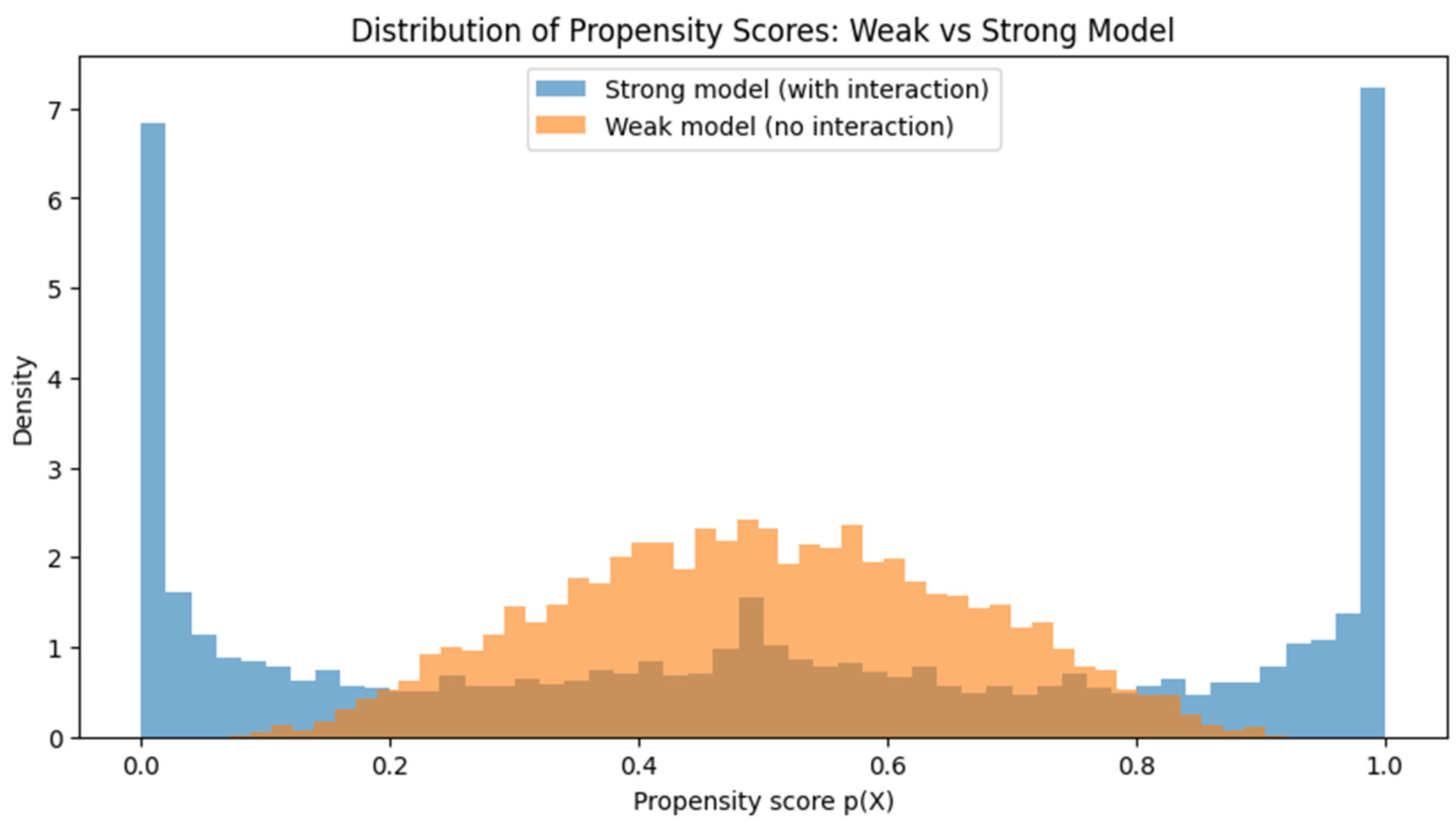
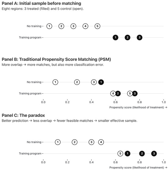
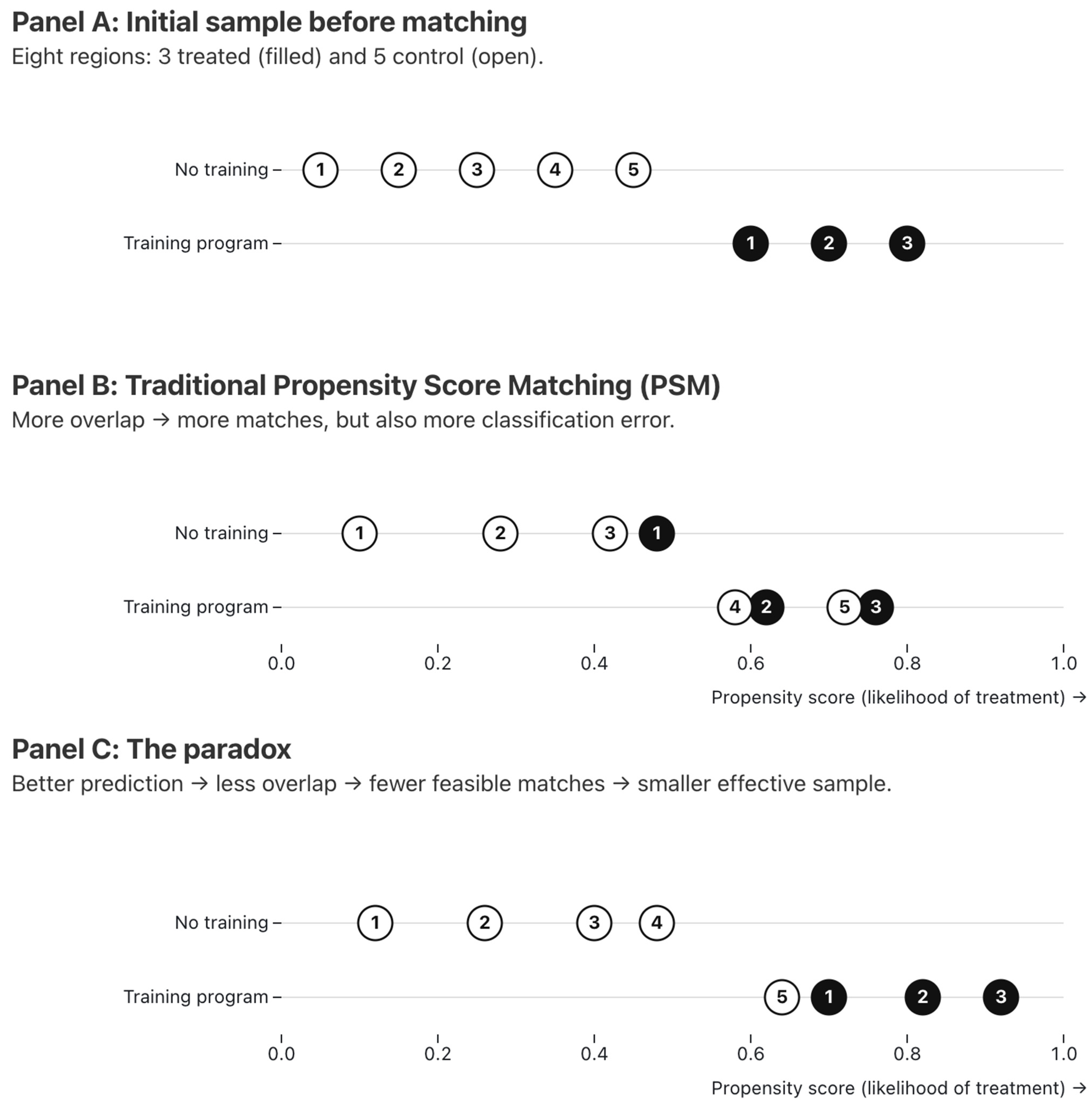
This paper argues, however, that improving predictive accuracy in propensity score models introduces a fundamental and underappreciated tension. As prediction becomes more accurate, estimated propensity scores for treated and control units become more distinct when treatment assignment is strongly predictable from observed covariates. In such settings, improved models reveal limited overlap, as treated and control units occupy increasingly separate regions of the propensity score distribution. Fewer units can be matched or retained after trimming, shrinking the effective sample size available for causal comparison. In extreme cases, highly accurate models approach complete separation, rendering traditional matching infeasible and confining any remaining inference to a narrow subset of units near the boundary of the propensity score distributions, a setting that is analogous to a regression discontinuity design. Figure 1 visualizes this separation directly, and Figure 2 shows how the same shift translates into fewer feasible matches in a simple matching schematic.
Figure 1.
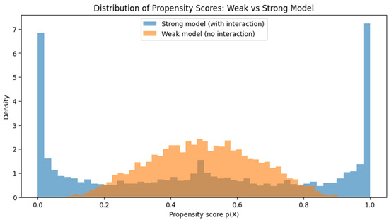
Distribution of estimated propensity scores: weak vs. strong model. Strong model (with interaction): Scores concentrate near 0 and 1, leaving little overlap between treated and control groups; This reduces usable sample size after trimming. Weak model (no interaction): Scores are more spread out in the middle, creating greater overlap; This allows more matches, but at the cost of model misspecification and bias. The predictability paradox: Stronger models are more accurate but leave fewer comparable units; Weaker models preserve overlap and matches but can introduce spurious bias.
Figure 2.
Predictability paradox: improved predictability reduces matches (schematic). Eight regions are shown: three treated (filled circles, ❶–❸; training program) and five controls (open circles, ①–⑤; no training). The horizontal axis reports each region’s estimated propensity score (probability of treatment). (Panel A) shows the initial sample before matching. (Panel B) illustrates traditional PSM under a relatively weak propensity score model: treated and control scores overlap, yielding three feasible matches (❶⟷③, ❷⟷④, ❸⟷⑤), but the overlap reflects nontrivial misclassification (false positives and false negatives). (Panel C) shows the same sample under a more accurate propensity score model: improved discrimination pushes treated scores higher and control scores lower, shrinking common support and leaving fewer feasible matches (here, only ❶⟷⑤), which reduces the matched sample size and weakens statistical power.
We refer to this tension as the predictability paradox: stronger propensity score models improve classification accuracy but simultaneously reduce overlap and statistical power. This paradox generates a perverse incentive structure. Researchers who prioritize statistically significant results may rationally prefer weaker, misspecified propensity score models that preserve overlap and sample size, even if those models yield biased estimates (Bruns and Ioannidis, 2016). By contrast, researchers who adopt more accurate models may be “punished” with smaller samples and null results, despite producing estimates that are closer to the true causal effect.
This incentive problem is especially troubling in policy-relevant research. Matching based on weak or noisy propensity scores can generate spuriously precise estimates that appear robust and statistically significant, yet are driven by residual confounding rather than causal effects. When such findings inform public policy decisions, the consequences can be substantial, particularly in domains such as environmental and public health policy where causal inference from observational data is central (e.g., Mork et al., 2024). For example, a policy intervention may appear effective simply because the propensity score model failed to capture the true determinants of treatment assignment, artificially inflating overlap between treated and untreated populations.
The predictability paradox identified here is distinct from existing critiques of propensity score matching. King and Nielsen (2019) argue that PSM can increase imbalance, model dependence, and bias relative to alternative matching methods, highlighting a trade-off between PSM and other approaches to preprocessing observational data. In contrast, this paper focuses on an internal trade-off within PSM itself: holding the matching framework fixed, improvements in predictive accuracy can undermine overlap, reduce effective sample size, and weaken statistical power. Studies advocating machine learning for propensity score estimation emphasize gains in bias reduction and covariate balance (Lee et al., 2010, in the context of propensity score weighting) without examining how improved prediction affects common support in matching contexts or generates perverse incentives to resist more accurate models. This paper bridges these two research fields by showing how improved prediction and limited overlap are mechanically linked.
Both Crump et al. (2009, p. 187) and Li et al. (2019, p. 250) observe, in strikingly similar terms, that causal estimation “is often hampered by” limited overlap. In each case, limited overlap is treated as an unfortunate feature of the data that complicates inference. Neither study considers that limited overlap might itself be a consequence of methodological improvement in propensity score estimation. This paper reframes the problem: what the prior literature characterizes as a data limitation can, under accurate prediction, be a direct and mechanical product of the researcher’s own modeling choices.
To illustrate this mechanism, the paper combines conceptual analysis and numerical simulation. A controlled simulation demonstrates that a weak, misspecified propensity score model can generate a statistically significant estimated treatment effect even when the true effect is zero, precisely because it preserves overlap and effective sample size. A stronger, correctly specified model eliminates this bias and correctly yields a smaller matched sample and a null result. The difference arises solely from predictive accuracy; the underlying data-generating process is held fixed.
Given these dynamics, the paper proposes a simple but consequential reform: studies using propensity score matching should be required to disclose basic measures of predictive performance, including false positive and false negative rates, along with information on overlap and effective sample size. Such disclosures would make transparent the trade-off between predictability and overlap, discourage strategic underfitting of propensity score models, and improve the reliability of evidence used in policy evaluation.
2. The Predictability Paradox: Conceptual Mechanism
Propensity score matching relies on a simple but demanding idea: treated and control units can be compared credibly if they have similar probabilities of receiving treatment, conditional on observed covariates. The propensity score compresses high-dimensional covariate information into a scalar measure of treatment likelihood, facilitating matching, weighting, or trimming in observational studies (Rosenbaum & Rubin, 1983). Central to the success of this approach is the existence of sufficient overlap, or common support, between the distributions of estimated propensity scores for treated and untreated units.
Machine learning methods seem like a natural fit here. They handle nonlinearities and interactions that logistic regression misses, and better prediction should, in principle, mean better-balanced matches. The problem is that sharper prediction also means sharper separation. As a model gets better at distinguishing treated from control units, it pushes their estimated scores toward opposite ends of the unit interval. The region where the two groups actually overlap shrinks. Matching and trimming procedures, which explicitly or implicitly restrict attention to the region of common support, therefore discard an increasing share of observations as predictive models improve, and the effective sample size available for causal inference shrinks even though the underlying data-generating process and total sample size remain unchanged. Figure 1 illustrates this compression toward the extremes under a stronger model, and Figure 2 provides a schematic version of the same logic, showing how improved discrimination can eliminate otherwise feasible matches. In the limiting case of near-perfect prediction, treated and control units become almost separable by a threshold in the estimated propensity score, rendering traditional matching difficult or infeasible and confining any remaining inference to a narrow subset of units near the boundary of the propensity score distributions.
This trade-off between predictive accuracy and overlap constitutes the predictability paradox. Stronger propensity score models reduce classification error but simultaneously reduce common support and effective sample size. Weaker models, by contrast, blur the distinction between treated and control units, preserving overlap and retaining more observations for analysis. Crucially, this preservation of overlap does not reflect improved comparability; rather, it arises from misspecification or underfitting that fails to capture the true treatment assignment mechanism.
The predictability paradox gives rise to a clear incentive problem. In environments where publication, funding, or policy impact depend heavily on statistical significance, researchers may face pressure to favor propensity score models that maintain large matched samples. Weaker models increase the likelihood of obtaining statistically significant estimates by inflating effective sample size, even if those estimates are biased due to residual confounding. Stronger, more accurate models may instead yield null results, not because the effect is absent, but because the correctly identified lack of overlap limits statistical power. This incentive structure is particularly concerning because standard reporting practices for propensity score matching rarely require authors to disclose predictive performance metrics such as false positive or false negative rates, nor do they consistently report how much of the original sample is discarded due to lack of common support, leaving readers, referees, and policymakers unable to assess whether a reported treatment effect reflects rigorous modeling or strategic underfitting.
It is important to distinguish the predictability paradox from existing critiques of propensity score matching. Ho et al. (2007) formalize matching as a nonparametric preprocessing step that improves covariate balance and reduces model dependence in subsequent parametric analyses, providing a framework that underlies later critiques of matching methods. Building on this framework, King and Nielsen (2019) argue that PSM can worsen imbalance, model dependence, and bias relative to alternative matching methods, emphasizing a trade-off between PSM and other approaches to preprocessing observational data. By contrast, the predictability paradox identified here arises within the PSM framework itself. Holding the matching procedure fixed, improvements in propensity score estimation can reduce overlap and statistical power. The paradox is therefore not an argument against matching per se, but against ignoring how predictive accuracy interacts mechanically with common support and inference.
Relatedly, prior work on limited overlap treats the problem as an unfortunate feature of the data: Crump et al. (2009) and Li et al. (2019) each acknowledge that estimation of average treatment effects is often “hampered” by limited overlap, yet neither considers that limited overlap might itself be a consequence of improved prediction. Conversely, studies advocating machine learning for propensity score estimation emphasize gains in bias reduction and covariate balance (Lee et al., 2010, in the context of propensity score weighting) without examining how improved prediction affects common support in matching contexts or generates perverse incentives to resist more accurate models. This paper connects these strands by showing that limited overlap can be induced by methodological improvements in prediction, thereby creating perverse incentives to resist those improvements.
How much this matters depends on the application. The paradox bites hardest when treatment is predictable from observed covariates, when the treated and control groups differ substantially in size, and when the researcher applies a strict caliper or trimming rule. All three conditions together can eliminate the majority of the sample. In settings where treatment assignment is weakly related to observed covariates, or where the researcher is willing to extrapolate using outcome regression, the problem is less severe. But those settings are arguably not the ones where matching is most needed in the first place. Importantly, these conditions can be partially diagnosed before committing to a modeling approach: examining the marginal distributions of key covariates by treatment status, inspecting the raw overlap in unadjusted propensity score distributions, and computing the AUC of a pilot model each provide early signals of how severely improved prediction is likely to compress common support.
3. Mathematical Framework
This section formalizes the mechanism underlying the predictability paradox described in Section 2. The goal is not to introduce a new estimator, but to clarify how improvements in predictive accuracy affect overlap, effective sample size, and statistical power in propensity score matching when the data-generating process is held fixed. Appendix A supplements this framework with a Gaussian logit parameterization that illustrates overlap decay as an explicit function of model separation and within-group variance, while otherwise restating the results of this section.
3.1. Setup and Notation
Let index observational units. Each unit is characterized by:
- a binary treatment indicator ,
- a vector of observed covariates ,
- an observed outcome .
Treatment assignment follows an unknown data-generating process summarized by the true propensity score
Outcomes are generated according to
where is the true average treatment effect, is an unknown function of covariates, and
Researchers do not observe and instead estimate propensity scores using a predictive model, yielding
We consider two classes of models:
- a weak (misspecified) model, producing ,
- a strong (well-specified or more flexible) model, producing .
The distinction between these models lies solely in predictive accuracy. The underlying population, treatment assignment process, and outcome equation are identical.
3.2. Overlap and Effective Sample Size
Define the empirical ranges of the estimated propensity scores among treated and control units as
The region of common support is given by
Matching, weighting, and trimming procedures explicitly or implicitly restrict attention to units whose estimated propensity scores lie in . Let denote the number of observations retained after this restriction.
As predictive accuracy improves, the distributions of estimated propensity scores for treated and control units typically become more separated. In expectation, stronger models tend to reduce the measure of common support relative to weaker models, even though strict set inclusion need not hold for any given realization. Consequently,
so that stronger models are associated with smaller effective sample sizes on average.
This reduction in effective sample size is mechanical. It arises from improved discrimination between treated and untreated units, not from changes in the data-generating process or from sampling variability.
3.3. Predictive Accuracy and Classification Error
To connect predictive accuracy to overlap, fix a classification threshold . Define the false positive and false negative rates as
Lower values of and correspond to higher predictive accuracy. As , there exists a threshold that increasingly separates treated and control units in terms of their estimated propensity scores. In this limit, the mass of observations in regions where treated and control units have similar estimated treatment probabilities becomes small, and the region of common support contracts.
Importantly, this contraction does not require overfitting or sampling noise. It can occur even under correct model specification and in large samples whenever treatment assignment is genuinely predictable given observed covariates.
3.4. Implications for Bias, Variance, and Power
Let denote an estimator of the average treatment effect based on matching or trimming using . Define bias as
Under standard conditions:
Weak models tend to preserve overlap and yield large effective sample sizes , but suffer from misspecification, so that
generally due to residual imbalance in functions of that affect outcomes. Strong models reduce misspecification and can substantially reduce bias
under correct specification of the propensity score and sufficient matching quality, but they typically do so at the cost of a smaller effective sample size .
The variance of generally increases as the effective sample size declines, and propensity score model overfitting can substantially inflate the variance of estimated effects, reducing precision (Schuster et al., 2016). Holding match quality and outcome variability fixed, a useful first-order approximation is
so reductions in overlap tend to inflate sampling variability. This expression abstracts from additional variance inflation that arises as propensity scores approach the boundaries of the support, where limited overlap and sparse matches reduce effective information; accounting for these effects would further strengthen the argument.
As a result, stronger models produce less biased but noisier estimates, while weaker models produce more precise but biased estimates. In finite samples, this trade-off directly affects statistical power. Biased estimates obtained under weak models may appear statistically significant due to large effective sample sizes, while less biased estimates under strong models may fail to reject the null because reduced overlap limits precision.
3.5. The Predictability Paradox
The predictability paradox emerges from the interaction of these elements:
- improved predictive accuracy reduces classification error,
- reduced classification error increases separation between treated and control units in propensity score space,
- increased separation reduces the mass of observations in regions of common support,
- reduced common support lowers effective sample size and statistical power.
This mechanism is model-agnostic. It arises from improved classification, not from any property of the functional form used to achieve that classification. Whenever a propensity score model, whether logistic regression, random forest, gradient boosted trees, or a neural network, more accurately distinguishes treated from control units, the estimated scores for the two groups become more separated in the unit interval. Common support contracts and effective sample size declines through the same channel described above, regardless of the estimator employed. Non-parametric machine learning methods are, if anything, more likely to induce the paradox in applied settings, precisely because they are capable of achieving substantially higher predictive accuracy in complex and high-dimensional covariate spaces. Researchers who adopt these methods specifically to improve propensity score estimation should therefore be especially attentive to the consequences for overlap and should apply the disclosure recommendations of Section 5 irrespective of the model class used.
This mechanism creates an implicit incentive to favor weaker, misspecified propensity score models that preserve overlap and yield statistically significant estimates, even when those estimates are biased. The paradox is therefore not a failure of matching itself, but a consequence of ignoring how predictive performance interacts mechanically with overlap and inference.
4. Illustration and Simulation Evidence
This section illustrates the predictability paradox in practice. We first present a simple illustrative example to build intuition. We then conduct a numerical simulation in which the data-generating process is held fixed while the researcher’s propensity score model varies in predictive accuracy. The simulation isolates how improved prediction affects overlap, effective sample size, and statistical inference in propensity score–based analyses.
4.1. An Illustrative Example
Consider a small sample of observational units, such as geographical regions, some of which receive a policy intervention (for example, a training or financial literacy program). The researcher observes a set of covariates and estimates a propensity score for each unit, representing the probability of receiving treatment conditional on those covariates.
In a typical empirical application, the estimated propensity scores of treated units tend to be higher than those of control units, but the distributions overlap. Matching proceeds by pairing treated and control units with similar estimated scores, often within a predefined caliper. Each match implicitly tolerates some degree of classification error: a treated unit matched to a control unit may reflect a false negative in the prediction model, while a control unit matched to a treated unit may reflect a false positive.
Now suppose the researcher replaces a simple parametric propensity score model with a more accurate machine learning model. As predictive performance improves, false positive and false negative rates decline. Mechanically, the estimated propensity scores of treated units move upward on average, while those of control units move downward on average. The region in which their scores overlap shrinks. Fewer units can be matched, and some treated units may have no comparable controls at all.
In the limiting case of near-perfect prediction, treated and control units become almost separable by a threshold in the estimated propensity score. Traditional matching becomes difficult or infeasible, and any remaining comparison relies on a narrow subset of observations near the boundary of the propensity score distributions. This example highlights the core mechanism of the predictability paradox: improved prediction reduces classification error but simultaneously reduces overlap.
4.2. Numerical Simulation
The simulation is a controlled illustrative exercise; the data-generating process is fully known, and the goal is to isolate the effect of predictive accuracy on overlap and inference rather than to optimize out-of-sample prediction. The simulation contrasts a weak, misspecified propensity score model with a stronger, correctly specified model. Crucially, the underlying data-generating process is identical across all exercises.
We generate a sample of observational units, indexed by .
Covariates. Each unit has two observed covariates,
independently distributed, and we write .
Treatment assignment. Treatment status is generated according to a nonlinear propensity score:
where the true propensity score is
The large interaction coefficient implies that treatment assignment is highly predictable when the interaction term is correctly modeled.
Outcome. Outcomes are generated as
where . The true average treatment effect is fixed at . Any nonzero estimated effect therefore reflects bias induced by model misspecification and selection through matching or trimming.
We consider two propensity score models that differ only in their ability to approximate the true treatment assignment mechanism.
Weak (misspecified) model. The weak model omits the interaction term and estimates
using a logistic regression with only main effects. This model is deliberately misspecified and exhibits poor classification performance.
Strong (well-specified) model. The strong model includes the interaction term and estimates
using a logistic regression with the correct nonlinear structure. This model achieves substantially higher predictive accuracy.
For each model, we proceed as follows.
First, we assess predictive performance using a fixed classification threshold of . We compute the false positive rate,
and the false negative rate,
These metrics summarize how well the model discriminates between treated and control units. The predictability paradox does not depend on the specific threshold chosen.
Second, we restrict the sample to the empirical region of common support, defined as the intersection of the ranges of estimated propensity scores among treated and control units.
Third, we estimate the average treatment effect as the difference in mean outcomes between treated and control units in the trimmed sample. Statistical significance is assessed using a Welch two-sample -test. This inference procedure is used for illustrative purposes; it does not account for dependence induced by trimming or matching.
The two models produce substantively different inferential conclusions despite operating on identical data and a known zero treatment effect.
Under the weak (misspecified) model, classification performance is poor, with a false positive rate of and a false negative rate of . Because the model fails to discriminate between treated and control units, the estimated propensity score distributions of the two groups remain substantially overlapping. Trimming removes few observations and the retained sample is nearly complete (). The estimated treatment effect is , which is statistically significant at conventional levels. This result is spurious: it arises from residual confounding due to model misspecification, not from a true causal effect.
Under the strong (well-specified) model, classification performance improves substantially, with a false positive rate of and a false negative rate of . The more accurate propensity score estimates produce greater separation between the score distributions of treated and control units. As a consequence, the region of common support contracts, and trimming removes a substantial share of the sample; the retained sample declines to , a reduction of more than 60 percent relative to the weak model. The estimated treatment effect falls to and is not statistically significant, correctly reflecting the true zero effect in the data-generating process.
These results illustrate the core incentive problem posed by the predictability paradox. The researcher using the correctly specified model obtains a smaller effective sample, wider confidence intervals, and a null result that accurately reflects the underlying data-generating process. The researcher using the misspecified model retains a larger sample, achieves a narrower confidence interval, and reports a statistically significant estimate of an effect that is, by construction, absent. The methodologically superior approach produces the less favorable outcome under prevailing publication norms.
5. Discussion and Conclusions
When readers, referees, and policymakers cannot observe how accurately a propensity score model predicts treatment assignment, they cannot evaluate whether a reported treatment effect reflects credible causal identification or the mechanical preservation of overlap by a misspecified model. The simulation in Section 4 makes this concrete: the only feature distinguishing a spurious, statistically significant result from a correct null is the accuracy of the propensity score model, and that accuracy is routinely undisclosed.
The contributions are threefold. First, the paper develops a clear conceptual and mathematical framework linking predictive accuracy, classification error, common support, and statistical inference in matching designs. Second, our numerical simulation demonstrates that weak propensity score models can generate statistically significant but spurious treatment effects even when the true effect is zero, which induces a perverse incentive to favor misspecification over accuracy under prevailing publication norms. Third, the paper proposes a simple and actionable reform.
Studies using propensity score matching should be required to disclose, at minimum: (1) false positive and false negative rates at a clearly stated classification threshold; (2) the area under the receiver operating characteristic curve; and (3) the proportion of the original sample retained after trimming or matching. These quantities are computable as a direct byproduct of any propensity score analysis. Their disclosure imposes negligible additional burden while providing readers with the information needed to distinguish rigorous modeling from strategic underfitting.
Each metric serves a distinct diagnostic purpose. False positive and false negative rates make classification error legible at a specific threshold. The AUC summarizes discrimination across all thresholds, rendering the assessment invariant to threshold choice; a value near 0.5 signals that overlap is being preserved by a model that is performing little better than chance. Together, these measures make the trade-off between predictive accuracy and common support visible rather than latent.
Disclosure of predictive performance must be accompanied by transparent reporting of overlap and effective sample size. Many published studies report only the final matched sample without indicating what share of the original sample was discarded. This practice conceals precisely the information that would allow a reader to assess whether large matched samples reflect genuine comparability or the tolerance of substantial misclassification. Unusually high retention rates combined with poor predictive performance should be treated as a warning sign, not evidence of methodological success.
A disclosure requirement mitigates the perverse incentive structure created by the predictability paradox. When error rates and trimming shares are visible, reviewers can more readily distinguish null results generated by credible, well-specified models from null results generated by excessive conservatism or limited data. Statistically significant results accompanied by poor classification performance and near-complete sample retention warrant closer scrutiny. Transparency does not eliminate the trade-off between accuracy and overlap; it prevents that trade-off from being exploited.
The policy stakes of this reform are substantial. Observational evidence from matching studies regularly informs decisions in health, education, labor markets, and financial regulation, domains in which randomized trials are often infeasible. When estimated treatment effects in these settings are driven by misspecified propensity score models rather than by genuine causal identification, the downstream consequences for resource allocation and program design can be considerable. The disclosure standards proposed here offer a low-cost mechanism for improving the evidentiary foundation on which such decisions rest.
The core insight is that matching is shaped as much by modeling choices as by the data themselves. As propensity score models become more accurate, they sharpen the separation between treated and control units, often shrinking the region of common support. This, in turn, affects the effective sample size and the conclusions that can be drawn from the design. In that sense, results from matching are not just properties of the data; they also reflect how treatment assignment is modeled. Thus, evidence from matching designs cannot be evaluated without information on predictive performance and overlap. Requiring routine disclosure of these quantities through journal reporting standards is a minimal and proportionate reform, but one that would materially improve the credibility and interpretability of empirical results used in policy decisions.
Funding
This research was funded by Willamette University (Atkinson Graduate School of Management), and Nanyang Technological University (NTU Singapore).
Institutional Review Board Statement
Not applicable.
Informed Consent Statement
Not applicable.
Data Availability Statement
The data are simulated, and full details are provided in the paper.
Acknowledgments
An earlier draft of this paper was presented at the 2022 American Accounting Association (AAA) Annual Meeting in San Diego. The author appreciates comments from the participants.
Conflicts of Interest
The author declares no conflict of interest.
Appendix A. Parametric Illustration of Overlap Decay Under Gaussian Logit Scores
The framework in Section 3 does not require distributional assumptions, but it can be useful to see the mechanism in closed form. We impose Gaussian logit scores here solely for that purpose. Readers who found Section 3 sufficient can skip this appendix; it adds no new results.
Appendix A.1. Setup and Notation
Let index observational units.
- denotes the treatment indicator for unit , where indicates treatment and indicates control.
- denotes the vector of observed covariates for unit .
- denotes the observed outcome.
The true propensity score is defined as
Researchers estimate the propensity score using a predictive model, yielding an estimated propensity score
As in the main text, we distinguish between:
- a weak (misspecified) model, producing estimates , and
- a strong (well-specified) model, producing estimates .
The outcome is generated according to
where is the true average treatment effect and .
Throughout, differences between weak and strong models arise solely from how accurately approximates ; the data-generating process itself does not change.
Appendix A.2. Overlap and Common Support
Define the empirical supports of the estimated propensity scores for treated and control units as
The region of common support is
Matching and trimming procedures restrict inference to units with . Let denote the number of units retained after trimming to common support.
As predictive accuracy improves, the distributions of for treated and control units become more separated in expectation. Strict sample-wise set inclusion need not hold in any given finite sample, because a single extreme observation can extend the empirical range of either group. The appropriate statement is therefore
so that stronger models are associated with smaller effective sample sizes on average.
Appendix A.3. Predictive Accuracy and Classification Error
Fix a classification threshold . Define:
- False positive rate
- False negative rate
Lower values of and correspond to higher predictive accuracy. The predictability paradox does not depend on the specific choice of ; the threshold is introduced solely for expositional clarity.
As predictive accuracy improves, , and estimated propensity scores approach perfect separation between treated and control units.
Appendix A.4. Predictive Separation and Shrinking Overlap
For analytical intuition, suppose that the logit-transformed estimated propensity scores satisfy
where . Working on the logit scale is consistent with the logit-scale calipers used in the matching procedure and avoids the boundary constraints of the unit interval.
Higher predictive accuracy corresponds to greater separation
and lower variance .
Under this approximation, the region of common support shrinks as increases and decreases. This approximation is used only to illustrate how improved prediction reduces overlap; the qualitative result does not depend on the distributional assumption.
Appendix A.5. Implications for Estimation and Power
Let denote the estimated average treatment effect obtained after matching or trimming based on . Define bias as
Then:
- Under weak models , misspecification preserves overlap but induces bias:
- Under strong models , bias is reduced:
Since
strong models may yield unbiased but imprecise estimates, while weak models may yield biased estimates that appear statistically significant due to inflated effective sample size.
Appendix A.6. The Predictability Paradox
Combining the above results yields the predictability paradox:
- Improved predictive accuracy reduces classification error ().
- Reduced error increases separation of estimated propensity scores.
- Separation shrinks the region of common support ().
- Shrinking support reduces effective sample size ().
- Reduced sample size weakens statistical power.
As a result, researchers may face incentives to favor weaker propensity score models that preserve overlap and yield statistically significant estimates, even though such estimates are biased. This paradox reflects an internal trade-off within matching designs between predictive accuracy and inferential reliability.
References
- Athey, S. (2018). The impact of machine learning on economics. In The economics of artificial intelligence: An agenda (pp. 507–547). University of Chicago Press. Available online: https://www.nber.org/system/files/chapters/c14009/c14009.pdf (accessed on 10 January 2026).
- Bruns, S. B., & Ioannidis, J. P. (2016). P-curve and p-hacking in observational research. PLoS ONE, 11(2), e0149144. [Google Scholar] [CrossRef] [Scilit] [PubMed]
- Carozza, S., Kletenik, I., Astle, D., Schwamm, L., & Dhand, A. (2025). Whole-brain white matter variation across childhood environments. Proceedings of the National Academy of Sciences, 122(15), e2409985122. [Google Scholar] [CrossRef] [Scilit] [PubMed]
- Crump, R. K., Hotz, V. J., Imbens, G. W., & Mitnik, O. A. (2009). Dealing with limited overlap in estimation of average treatment effects. Biometrika, 96(1), 187–199. [Google Scholar] [CrossRef] [Scilit]
- Goller, D., Lechner, M., Moczall, A., & Wolff, J. (2020). Does the estimation of the propensity score by machine learning improve matching estimation? The case of Germany’s programmes for long term unemployed. Labour Economics, 65, 101855. [Google Scholar] [CrossRef] [Scilit]
- Ho, D. E., Imai, K., King, G., & Stuart, E. A. (2007). Matching as nonparametric preprocessing for reducing model dependence in parametric causal inference. Political Analysis, 15(3), 199–236. [Google Scholar] [CrossRef] [Scilit]
- Jiang, R., Geha, P., Rosenblatt, M., Wang, Y., Fu, Z., Foster, M., Dai, W., Calhoun, V. D., Sui, J., Spann, M. N., & Scheinost, D. (2025). The inflammatory and genetic mechanisms underlying the cumulative effect of co-occurring pain conditions on depression. Science Advances, 11(14), eadt1083. [Google Scholar] [CrossRef] [Scilit] [PubMed]
- King, G., & Nielsen, R. (2019). Why propensity scores should not be used for matching. Political Analysis, 27(4), 435–454. [Google Scholar] [CrossRef] [Scilit]
- Lee, B. K., Lessler, J., & Stuart, E. A. (2010). Improving propensity score weighting using machine learning. Statistics in Medicine, 29(3), 337–346. [Google Scholar] [CrossRef] [Scilit] [PubMed]
- Li, F., Thomas, L. E., & Li, F. (2019). Addressing extreme propensity scores via the overlap weights. American Journal of Epidemiology, 188(1), 250–257. [Google Scholar] [CrossRef] [Scilit] [PubMed]
- Mork, D., Delaney, S., & Dominici, F. (2024). Policy-induced air pollution health disparities: Statistical and data science considerations. Science, 385(6707), 391–396. [Google Scholar] [CrossRef] [Scilit] [PubMed]
- Mullainathan, S., & Spiess, J. (2017). Machine learning: An applied econometric approach. Journal of Economic Perspectives, 31(2), 87–106. [Google Scholar] [CrossRef] [Scilit]
- Rosenbaum, P. R., & Rubin, D. B. (1983). The central role of the propensity score in observational studies for causal effects. Biometrika, 70(1), 41–55. [Google Scholar] [CrossRef]
- Schuster, T., Lowe, W. K., & Platt, R. W. (2016). Propensity score model overfitting led to inflated variance of estimated odds ratios. Journal of Clinical Epidemiology, 80, 97–106. [Google Scholar] [CrossRef] [Scilit] [PubMed]
- Shipman, J. E., Swanquist, Q. T., & Whited, R. L. (2017). Propensity score matching in accounting research. The Accounting Review, 92(1), 213–244. [Google Scholar] [CrossRef] [Scilit]
Disclaimer/Publisher’s Note: The statements, opinions and data contained in all publications are solely those of the individual author(s) and contributor(s) and not of MDPI and/or the editor(s). MDPI and/or the editor(s) disclaim responsibility for any injury to people or property resulting from any ideas, methods, instructions or products referred to in the content. |
© 2026 by the author. Licensee MDPI, Basel, Switzerland. This article is an open access article distributed under the terms and conditions of the Creative Commons Attribution (CC BY) license.