Propensity Score and the Double Robust Estimator in the Tails

Abstract

This study analyzes the performance of the double robust estimator to compute the treatment effect, not only at the mean but also in the tails in a Monte Carlo experiment. While previous research focused on shifting the regression component of the double robust estimator toward the tail, here we focus on the behavior of the propensity score away from the mean. Investigating the tails of the regression outcome allows for a closer look at the observations that are either highly or poorly responsive to treatment. Examining the tails of the propensity score distribution scrutinizes the observations with a higher or lower probability of being treated, which can be non-constant and even asymmetric. The goal is to assess the behavior of the double robust estimator when both components are computed away from the sample mean, in the tails of the treatment and control distributions. A case study on Italian education concludes the analysis. We find a positive double robust difference in higher education across regions, larger at the top location, due to the significant internal migration of qualified workers toward the northern regions. Women’s employment is higher for highly educated women, and gender has a significant impact: the analysis of the mismatch between probabilities and outcomes signals that women achieve higher education at rates exceeding their probabilities; they are more likely to exceed their predicted likelihood of attaining higher education.

1. Introduction

The double robust estimator (Lunceford & Davidian, 2004) computes the average treatment effect by focusing on two components, the propensity score (PS) and the OLS regression estimates. PS (Rosenbaum & Rubin, 1983; Naimi & Whitcomb, 2023) estimates the probability of belonging to the treatment group conditionally on the covariates. The observations are weighted by the inverse probability of being treated. The weighted observations define the potential outcomes representing the hypothetical outcomes that would occur under different exposure, i.e., possible and not observed exposure. The comparison of the potential outcome of treated and control provides an estimate of the treatment effect as estimated at the mean. The aim is to control the potential bias that arises when treated individuals systematically differ from the untreated.1 The OLS regression provides the other component of the double robust estimator (DR) and relates individuals’ outcomes to a set of explanatory variables to compute the unconditional distribution of the dependent variable. The OLS fitted values distinctly estimated in the treated and in the control groups are compared, providing an evaluation of the treatment effect (Neugebauer & van der Laan, 2005).

DR combines propensity scores and OLS fitted values. The comparison of treated and untreated in both components computes the DR average treatment effect. DR is a consistent estimator if at least one of these two components is correctly specified. However, heterogeneous impacts of the treatment along the distribution may arise. Heterogeneity may occur in any of the two components, in the probability of being treated, the PS, or in the regression model. In case of heterogeneity in one or both components of DR, the average is a poor approximation of the True Treatment Effect since an average value misrepresents the tail behavior.

The emphasis here is on estimating treatment effect not only at the mean but also across the tails, at multiple locations, i.e., measuring the quantile treatment effect.2

Caracciolo and Furno (2017) propose to analyze a binary treatment effect at the quantiles by introducing a quantile regression estimator in place of OLS. The impact on the tails may differ from the treatment estimated on average: additional schooling may grant better jobs and higher earnings in the upper tail than on average or at the lower tail. It may be the case that the impact of treatment differs across the distribution, being negative at the lower and positive at the upper quantiles, while offsetting at the mean. By introducing the quantile regression estimated outcomes in each group, Caracciolo and Furno (2017) estimate the treatment effect even in the tails of the outcome distribution.3 They move the estimated regression away from the mean, computing the unconditional distribution of the outcome and looking at the quantiles while keeping the PS estimates constant at the conditional mean. This implies the exclusion, by assumption, of any heterogeneity in the probability of treatment and in the PS. This probability may change as well, as is the case with an asymmetric probability distribution. For instance, the odds in favor of additional schooling can be higher at lower quantiles or at the top ones. Analogously, the probability of women’s employment can be lower in the left tail for low-qualified jobs and higher in the right tail (Picchio & Mussida, 2011).

In this study, PS is not constant and is estimated at the mean and in the tails. The focus is on the probability of being in one group or another at and away from the mean. Thus, the DR estimator is computed by moving both components to the tail, propensity score, and regression model. The propensity score in the tail is coupled with the quantile regression estimates at the same location to provide a tail estimator with respect to both components of the double robust estimator, the propensity score and the regression model. The attempt is to explain a changing probability together with a changing outcome, i.e., considering the observations with a greater/lower probability of being treated and highly/poorly responsive to treatment. Looking at the tails of the regression component implies considering the behavior of the more responsive observations with respect to the treatment. Looking at the tails of the propensity score distribution analyzes an asymmetric and not constant probability of being treated. The novelty of the following approach is in considering the mixing of potential outcome and regression approach of the double robust estimator at the center and in the tails of both DR components to compute the quantile treatment effect. The knowledge of the response to a changing probability is a relevant issue, just as the response of the regression component of DR.

It is also possible to analyze the two DR components at different locations, as will be seen in the case study. Selecting different locations in the DR components would model observations with a high probability of treatment coupled with low treatment levels, and vice versa, low probability coupled with high results. This would crush the double robustness of the estimator, but it helps model mismatches between probabilities and results: individuals with a high probability of training working in non-specialized, low-paid jobs, and vice versa.

The results of a small Monte Carlo study show that in the case of a constant probability of treatment, it is irrelevant to analyze the propensity score in the tails as discussed so far. When the treatment odds are not constant and/or skewed, it is better to move the propensity score away from the mean at the selected location of interest, and the DR estimator here analyzed is of use to investigate a treatment effect in the tail.

A real data example of 2020 Italian data concludes the analysis. Gender and, in turn, region of residence are considered as a source of group heterogeneity in completing higher education. The results show that women and, in turn, people living in the northern regions attain higher education: there is a larger number of highly educated women with respect to men, and there is a prevalence of highly educated people residing in the northern regions. The former can be explained by the generally lower rate of women’s employment, particularly in lower-skilled jobs. The latter can be explained by the significant internal migration toward the northern regions, mainly for qualified workers, due to more favorable job market conditions in these economically richer regions. Additionally, we model the case of a different location between probability and quantile regression within the double robust approach: highly educated people, at the top regression quantile, characterized by a low probability of higher education, or vice versa, people unfulfilling their probability of higher education. In this data set, the analysis of the mismatch between probabilities and outcomes signals that women attain higher education at rates exceeding their probabilities. Thus, gender has a significant impact on attaining higher education, even if the probability of higher education is not very large, and women are more likely to outperform relative to expectations, attaining higher education at rates that exceed their predicted probabilities.

Besides the approach here discussed, there are, of course, many other differing estimators for quantile regression and double robustness. The DR marginal structure quantile model considers the causal effect of a time-varying treatment on the full distribution of potential outcomes (Cheng et al., 2022). Their estimator combines a treatment model with an outcome distribution model and attains semiparametric efficiency when both are correct. It is relevant when the goal is quantile treatment effects with protection against misspecification. Its building block is the efficient influence function (Cattaneo, 2010). The latter introduces a correcting term to remove bias and improve efficiency. The augmentation component uses outcome predictions to fix bias and improve efficiency, enabling double robustness.

The overlap weighted approach is defined for heterogeneous treatment effects (Akinshin, 2023) and implements weighting schemes to improve finite sample stability. Overlap weighting produces bounded, stable weights and targets the treatment effect in the overlap population, i.e., it considers a subgroup of the sample to reduce heterogeneity.

All these estimators rely on the inverse probability weights as computed at the mean by the standard logit model. They do not consider skewed or changing treatment odds and compute propensity scores at the mean. Vice versa, we do allow for changing probability, and our attempt is to capture it by moving the logit estimates away from the mean.

The recentered influence functions (Firpo et al., 2009) are closely related to the efficient influence function and analyze unconditional quantile regressions.

Finally, heavy tails and tail instability cause inefficiency. Trimming or truncating to remove extreme propensity scores, or smoothing approaches that regularize the quantile function, are frequently used in the literature. These approaches can be embedded within double robust methods, although they involve a bias-efficiency trade-off.

2. The Estimator

Consider the outcome variable Y_i, which assumes value Y_i0 in the control group if the treatment variable Z_i is 0 and Y_i1 when the treatment variable assumes unit value, Z_i = 1 for treatment, in a sample of size n. To measure the average treatment effect, DR combines the propensity score and regression approach. Under the assumption of independence between (Y_i0, Y_i1) and the explanatory variables in X (Lunceford & Davidian, 2004), the double robust estimator is

$${\mathrm{n}}^{-1}[{\sum }_{\mathrm{i}=1}^{\mathrm{n}}(\frac{{\mathrm{Z}}_{\mathrm{i}}{\mathrm{Y}}_{\mathrm{i}}}{\mathrm{P}({\mathrm{Z}}_{\mathrm{i}}=1|\mathbf{X})}-\frac{{\mathrm{Z}}_{\mathrm{i}}-\mathrm{P}({\mathrm{Z}}_{\mathrm{i}}=1|\mathbf{X})}{\mathrm{P}({\mathrm{Z}}_{\mathrm{i}}=1|\mathbf{X})} {\hat{\mathrm{Y}}}_{\mathrm{i}1})-{\sum }_{\mathrm{i}=1}^{\mathrm{n}}(\frac{{(1-\mathrm{Z}}_{\mathrm{i}}){\mathrm{Y}}_{\mathrm{i}}}{1-\mathrm{P}({\mathrm{Z}}_{\mathrm{i}}=1|\mathbf{X})}+\frac{{\mathrm{Z}}_{\mathrm{i}}-\mathrm{P}({\mathrm{Z}}_{\mathrm{i}}=1|\mathbf{X})}{1-\mathrm{P}({\mathrm{Z}}_{\mathrm{i}}=1|\mathbf{X})} {\hat{\mathrm{Y}}}_{\mathrm{i}0})]$$

(1)

where the propensity score provides the probability weights P(Z_i = 1|X), with 0 < P(Z_i = 1|X) < 1, i.e., the probability of treatment given the observed matrix of covariates X. It is estimated by assuming that P(Z_i = 1|X) follows a parametric model, a logistic regression

$$\mathrm{P}(Z_i=1|\mathbf{X})=\frac{\mathrm{e}\mathrm{x}\mathrm{p}\left(\mathbf{X}\mathsf{\beta }\right)}{\{1+\mathrm{e}\mathrm{x}\mathrm{p}(\mathbf{X}\mathsf{\beta }\left)\right\}}$$

(2)

The probability of being treated provides the weights to compute the potential outcome. The outcome Y_i is weighted by the inverse of this probability, respectively $\frac{{\mathrm{Z}}_{\mathrm{i}}{\mathrm{Y}}_{\mathrm{i}}}{\left({\mathrm{Z}}_{\mathrm{i}}=1\right|\mathbf{X})}=\frac{{\mathrm{Y}}_{\mathrm{i}}}{\mathrm{P}\left({\mathrm{Z}}_{\mathrm{i}}=1\right|\mathbf{X})}$ for the treated, where Z_i = 1, and $\frac{(1-{\mathrm{Z}}_{\mathrm{i}}){\mathrm{Y}}_{\mathrm{i}}}{1-\mathrm{P}\left({\mathrm{Z}}_{\mathrm{i}}=1\right|\mathbf{X})}=\frac{{\mathrm{Y}}_{\mathrm{i}}}{1-\mathrm{P}\left(\mathrm{Z}=1\right|\mathbf{X})}$ for the untreated with Z_i = 0.

Equation (1) takes the difference between treated and control: in the treatment group, when Z_i = 1, it compares weighted observed and fitted values of the regression, respectively Y_i and ${\hat{\mathrm{Y}}}_{\mathrm{i}1}$ with weights equal to $\frac{1}{\mathrm{P}({\mathrm{Z}}_{\mathrm{i}}=1|\mathbf{X})}$ and $\frac{\mathrm{P}({\mathrm{Z}}_{\mathrm{i}}=0|\mathbf{X})}{\mathrm{P}({\mathrm{Z}}_{\mathrm{i}}=1|\mathbf{X})}$

$${\mathrm{n}}^{-1}\left[\sum (\frac{{\mathrm{Y}}_{\mathrm{i}}}{\mathrm{P}({\mathrm{Z}}_{\mathrm{i}}=1|\mathbf{X})}-\frac{1-\mathrm{P}({\mathrm{Z}}_{\mathrm{i}}=1|\mathbf{X})}{\mathrm{P}({\mathrm{Z}}_{\mathrm{i}}=1|\mathbf{X})} {\hat{\mathrm{Y}}}_{\mathrm{i}1})-\sum {\hat{\mathrm{Y}}}_{\mathrm{i}0}\right] \mathrm{for} {\mathrm{Z}}_{\mathrm{i}}=1$$

(3)

while in the control group, when Z_i = 0, Y_i is weighted by $\frac{1}{\mathrm{P}({\mathrm{Z}}_{\mathrm{i}}=0|\mathbf{X})}$ and ${\hat{\mathrm{Y}}}_{\mathrm{i}0}$ is weighted by $\frac{\mathrm{P}({\mathrm{Z}}_{\mathrm{i}}=1|\mathbf{X})}{\mathrm{P}({\mathrm{Z}}_{\mathrm{i}}=0|\mathbf{X})}$, as follows

$${\mathrm{n}}^{-1}\left[\sum {\hat{\mathrm{Y}}}_{\mathrm{i}1}-\sum (\frac{{\mathrm{Y}}_{\mathrm{i}}}{1-\mathrm{P}({\mathrm{Z}}_{\mathrm{i}}=1|\mathbf{X})}-\frac{\mathrm{P}({\mathrm{Z}}_{\mathrm{i}}=1|\mathbf{X})}{1-\mathrm{P}({\mathrm{Z}}_{\mathrm{i}}=1|\mathbf{X})} {\hat{\mathrm{Y}}}_{\mathrm{i}0})\right] \mathrm{for} {\mathrm{Z}}_{\mathrm{i}}=0$$

(4)

Next, we look at the propensity score estimator away from the conditional mean. The logistic quantile regression models continuous outcomes that are bounded within a known interval, i.e., (0,1) for probabilities. It can be defined as P(Z_i) ∈ (P(Z_min), P(Z_max)), where P(Z_min) and P(Z_max) are the limits of the outcome variable, P(Z_i) ∈ (0,1) for probability. For any quantile θ, there exists a fixed set of regression parameters β_θ and a non-decreasing function h such that h(P(Z(θ))) = x_i′β_θ, where x_i′ is the row vector comprising the ith observations of the explanatory variables in X. Among a variety of suitable choices for h, there is the logistic transformation (Machado & Santos-Silva, 2008; Bottai et al., 2010). However, this estimator is consistent only under homoskedasticity (Huber & Melly, 2015; Fitzenberger & de Lazzer, 2022). This assumption is not very useful in our analysis, where the goal is to detect changing/heterogeneous and skewed treatment odds. Therefore, we consider expectiles to provide a shifting weight that moves the estimated logistic regression away from the conditional mean.4 Indeed, the expectile estimator (Newey & Powell, 1987) is not restricted to homoscedasticity and is defined as an asymmetrically weighted regression where the weights set the location of the estimated equation. Its drawback is its lack of robustness, and this would cause biased estimates in the presence of anomalous values in the sample. Equation (2) is modified to include an asymmetric weighting system that moves the equation up or down toward the tails:

$${\mathrm{w}}_{\mathrm{i}}{\mathrm{Z}}_{\mathrm{i}}={\mathrm{w}}_{\mathrm{i}}\frac{\mathrm{e}\mathrm{x}\mathrm{p}\left(\mathbf{X}\mathsf{\beta }\right)}{\{1+\mathrm{e}\mathrm{x}\mathrm{p}(\mathbf{X}\mathsf{\beta }\left)\right\}}$$

(5)

where the asymmetric weighting system is ${\mathrm{w}}_{\mathrm{i}}=\{\begin{array}{c}\mathsf{\theta }ifu>0\\ 1-\mathsf{\theta }elsewhere\end{array}$.

• u is the residual in the logistic regression and θ the selected location. For instance, to compute the θ = 25th expectile, ${\mathrm{w}}_{\mathrm{i}}$ assigns weights of 0.75 to those observations below the regression to attract the estimated equation toward the lower tail and assigns weights of 0.25 to the observations above it.

Turning to the regression component, the ${\hat{\mathrm{Y}}}_{\mathrm{i}1}$ and ${\hat{\mathrm{Y}}}_{\mathrm{i}0}$ in Equations (3) and (4), the fitted values of the regression model Y_ij = Xα + e_i are computed in each group, for j = 0, 1, with Y being the outcome and X the matrix of explanatory variables. The terms ${\hat{\mathrm{Y}}}_{\mathrm{i}0}$ and ${\hat{\mathrm{Y}}}_{\mathrm{i}1}$ are estimated by the unconditional distributions of the fitted values within each group, from now on ${\widehat{\tilde{\mathrm{Y}}}}_{\mathrm{i}1}$ and ${\widehat{\tilde{\mathrm{Y}}}}_{\mathrm{i}0}$. Indeed, while with OLS, conditional and unconditional effects coincide in moving to the tails, i.e., in the quantile regression framework, their interpretation is slightly different due to the definition of the quantile (Frolich & Melly, 2010).5

To compute the unconditional distributions, the approach discussed by Melly (2006) is here implemented. First, the conditional distributions of the dependent variables are estimated by quantile regression (Koenker, 2005) at many quantiles (k = 100), distinctly in the treated and in the control group, by the following objective function

$${\sum }_{\mathrm{Y}>\mathbf{X}\mathsf{\alpha }}\mathsf{\theta }\left|\mathrm{Y}-\mathbf{X}\mathsf{\alpha }\right|+{\sum }_{\mathrm{Y}<\mathbf{X}\mathsf{\alpha }}(1-\mathsf{\theta })\left|\mathrm{Y}-\mathbf{X}\mathsf{\alpha }\right|$$

(6)

where $\mathsf{\theta }$ is the selected quantile and $\mathrm{Y}-\mathbf{X}\mathsf{\alpha }$ are the linear regression errors.

The analysis within each group yields two sets of estimated coefficients, ${\hat{\mathsf{\alpha }}}_1\left(\mathsf{\theta }\right)$ for the treated group and ${\hat{\mathsf{\alpha }}}_0(\mathsf{\theta })$ for the control. The corresponding fitted values, ${\hat{\mathrm{Y}}}_{\mathrm{i}0}\left(\mathsf{\theta }\right)|{\mathbf{X}}_0={\mathbf{X}}_0{\hat{\mathsf{\alpha }}}_0\left(\mathsf{\theta }\right)$ and ${\hat{\mathrm{Y}}}_{\mathrm{i}1}\left(\mathsf{\theta }\right)|{\mathbf{X}}_1={\mathbf{X}}_1{\hat{\mathsf{\alpha }}}_1\left(\mathsf{\theta }\right)$, provide the distribution of the outcome at a given quantile, conditional on the set of covariates X in each group. The estimation of k different quantile regressions within each group yields k values of ${\widehat{\tilde{\mathsf{\alpha }}}}_0\left(\mathsf{\theta }\right)$ and of ${\widehat{\tilde{\mathsf{\alpha }}}}_1\left(\mathsf{\theta }\right)$. The covariates are bootstrapped within each group as well, yielding k samples of ${\tilde{\mathbf{X}}}_0$ and of ${\tilde{\mathbf{X}}}_1$. By bootstrapping the covariates and the coefficients within each group, it is possible to compute the unconditional distributions of the dependent variable for treated and untreated by ${\widehat{\tilde{\mathrm{Y}}}}_{\mathrm{i}0}={\tilde{\mathbf{X}}}_0{\widehat{\tilde{\mathsf{\alpha }}}}_0\left(\mathsf{\theta }\right)$ and ${\widehat{\tilde{\mathrm{Y}}}}_{\mathrm{i}1}={\tilde{\mathbf{X}}}_1{\widehat{\tilde{\mathsf{\alpha }}}}_1\left(\mathsf{\theta }\right)$.6 These terms take the place of the OLS fitted values ${\hat{\mathrm{Y}}}_{\mathrm{i}0}$ and ${\hat{\mathrm{Y}}}_{\mathrm{i}1}$ in Equation (1) as follows

$$\mathrm{Q}[(\frac{{\mathrm{Z}}_{\mathrm{i}}{\mathrm{Y}}_{\mathrm{i}}}{\mathrm{P}\left({\mathrm{Z}}_{\mathrm{i}}=1\right|\mathbf{X})}-\frac{{\mathrm{Z}}_{\mathrm{i}}-\mathrm{P}\left({\mathrm{Z}}_{\mathrm{i}}=1\right|\mathbf{X})}{\mathrm{P}\left({\mathrm{Z}}_{\mathrm{i}}=1\right|\mathbf{X})} {\widehat{\tilde{\mathrm{Y}}}}_{\mathrm{i}1})-(\frac{{(1-\mathrm{Z}}_{\mathrm{i}}){\mathrm{Y}}_{\mathrm{i}}}{1-\mathrm{P}\left({\mathrm{Z}}_{\mathrm{i}}=1\right|\mathbf{X})}+\frac{{\mathrm{Z}}_{\mathrm{i}}-\mathrm{P}({\mathrm{Z}}_{\mathrm{i}}=1|\mathbf{X})}{1-\mathrm{P}({\mathrm{Z}}_{\mathrm{i}}=1|\mathbf{X})} {\widehat{\tilde{\mathrm{Y}}}}_{\mathrm{i}0})]$$

(7)

and the probability weights $\mathrm{P}\left({\mathrm{Z}}_{\mathrm{i}}=1\right|\mathbf{X})$ and 1 − $\mathrm{P}\left({\mathrm{Z}}_{\mathrm{i}}=1\right|\mathbf{X})$ are computed as in Equation (5). Equation (7) computes DR at any selected quantile Q, away from the mean.

3. Simulations

The simulations are computed in Stata, version 16. The analyzed model is defined as

$$y_{ij}={\beta }_1+{\beta }_2{x}_{2ij}+{\beta }_3{x}_{3ij}+{\epsilon }_{ij},\hspace{1em}i=1,\dots ,n;j=0,1$$

(8)

the $\mathit{\beta }$ vector assumes values (${\beta }_1$, ${\beta }_2$, ${\beta }_3$)′ = (4, 2, 1)′; $x_{2ij}$ is a standard normal independent of ${\epsilon }_i$; $x_{3ij}$ is a binomial B(100; 0.5); the sample size is n = 500, and there are 500 iterations for each experiment. The experiments consider the effect of a treatment by defining the error term ${\epsilon }_i$ as an asymmetric mixture of normal distributions. The positive values in the right tail of a standard normal are replaced by the absolute value of the realizations of a normal distribution centered on 100 and having unit variance. This entails a treatment having a 50% rate of success, where treatment has a positive impact and increases the outcome by 100, since the impact of treatment is equal to the mean of the contaminating distribution, 100. Analogously, a treatment reducing the impact—for instance, a new medical treatment to lower cholesterol/toxicity/cancerous cells—can be modeled by replacing the left tail of a standard normal. We compute treatment at the center, at the 75th, and at the 95th location. Then, a 30% impact of treatment is considered by replacing only 30% of the values in the right tail of the standard normal with the absolute values of a normal centered on 100. Finally, an even smaller treatment effect is considered by setting 30% of treatment impact and reducing the mean of the treatment to 50.

The treatment effect has a twofold aspect: (i) its extent in improving performance and (ii) the percentage of observations involved. The percentage in the first set of experiments is a function of a uniform defined in the [0; 1] interval, Uniform [0; 1] in the table. The observations belong to the treated group if the realizations of the uniform are greater than or equal to 0.5. This implies that 50% of the sample is being treated, and all the observations have the same treatment odds. In a second set of experiments, the probability of being treated is non-constant and is a function of a standard normal. Treatment is assigned to the non-negative realizations of a standard normal. It still comprises 50% of the sample, but the probability of treatment is no longer constant. Finally, we consider a longer right-tail distribution to model a non-constant and asymmetric probability of treatment. Treatment odds are modeled by a 10% unilaterally contaminated normal where the upper 10% of the right tail is replaced by a uniform distribution defined in the [0; 5] interval.

In the above experiments, the simulations focus on the PS component, distributed as a uniform, a standard normal, and a contaminated normal. In each set of experiments, PS has been computed beyond the mean by weighting the observations to move the estimates toward the right tail, at the 75th and 95th locations. The very last experiment, instead, considers normal and contaminated normal distributions in the probability of treatment, but the latter is computed only at the mean. The same PS as estimated at the mean is implemented in computing DR at the 75th and 95th locations. This would check the behavior of DR when a non-constant and a skewed probability of treatment are foregone.7 The case of a small treatment effect is analyzed, where treatment is equal to 50 and impacts only 30% of the sample.

4. Results

Table 1. Summary statistics of the DR Estimated Treatment Effect at various locations: treatment effect equal to 100 involving 50% of the sample.

	50th	75th	95th
	sample mean	sample mean	sample mean
True Treatment Effect	99.897	100.937	102.214
Standard deviation	(0.072)	(0.033)	(0.017)
Probability of treatment	Uniform [0; 1]
Estimated Treatment Effect	−0.001	51.884	102.320
Standard deviation RMSE	St. dev. = 0.233 RMSE = 44.45	St. dev. = 48.072 RMSE = 49.25	St. dev. = 0.675 RMSE = 0.66
Probability of treatment	Standard normal
Estimated Treatment Effect	100.978	101.599	102.422
Standard deviation RMSE	St. dev. = 0.095 RMSE = 51.46	St. dev. = 0.094 RMSE = 1.61	St. dev. = 0.120 RMSE = 0.62
Probability of treatment	Contaminated normal
Estimated Treatment Effect	100.999	101.610	102.437
Standard deviation	St. dev. = 0.103 RMSE = 53.06	St. dev. = 0. 105 RMSE = 1.61	St. dev. = 0.128 RMSE = 0.63

reports the sample means and the standard deviations of the empirical distributions of the treatment effect as computed by implementing the DR estimator of Equation (7), Estimated Treatment Effect in the table. These values are compared with the True Treatment Effect reported at the top of the table. The latter is computed by comparing treated and control distributions as follows: the control group, $y_{i0}$, is defined as in Equation (8), and the errors follow a standard normal distribution; the error term of the treated, $y_{i1}$, is defined instead by a normal with mean 100, N [100; 1]. The difference between treated and untreated is computed, and the 50th, the 75th, and, in turn, the 95th quantiles are computed. These values provide the benchmarks to evaluate the behavior of DR under the designated regimes of sample selection.

Table 1 collects the results of a 50% impact of treatment, having a mean of 100 in the case of uniform, standard normal, and contaminated normal treatment odds. The experiments with a uniform probability of treatment show the inability of DR to capture treatment effect: at the median, the DR empirical distribution is centered on zero; at the 75th location, it is centered on 51 and is highly dispersed; only in the far tail, at the 95th location, does DR compute the True Treatment Effect and have a small dispersion. When the probability of treatment is no longer constant and follows a standard normal or a contaminated normal distribution, as in the last two sections of this table, DR results are very close to the true effect, with a very slight overestimation and a small dispersion. The latter slightly increases moving to the tail, at 95.

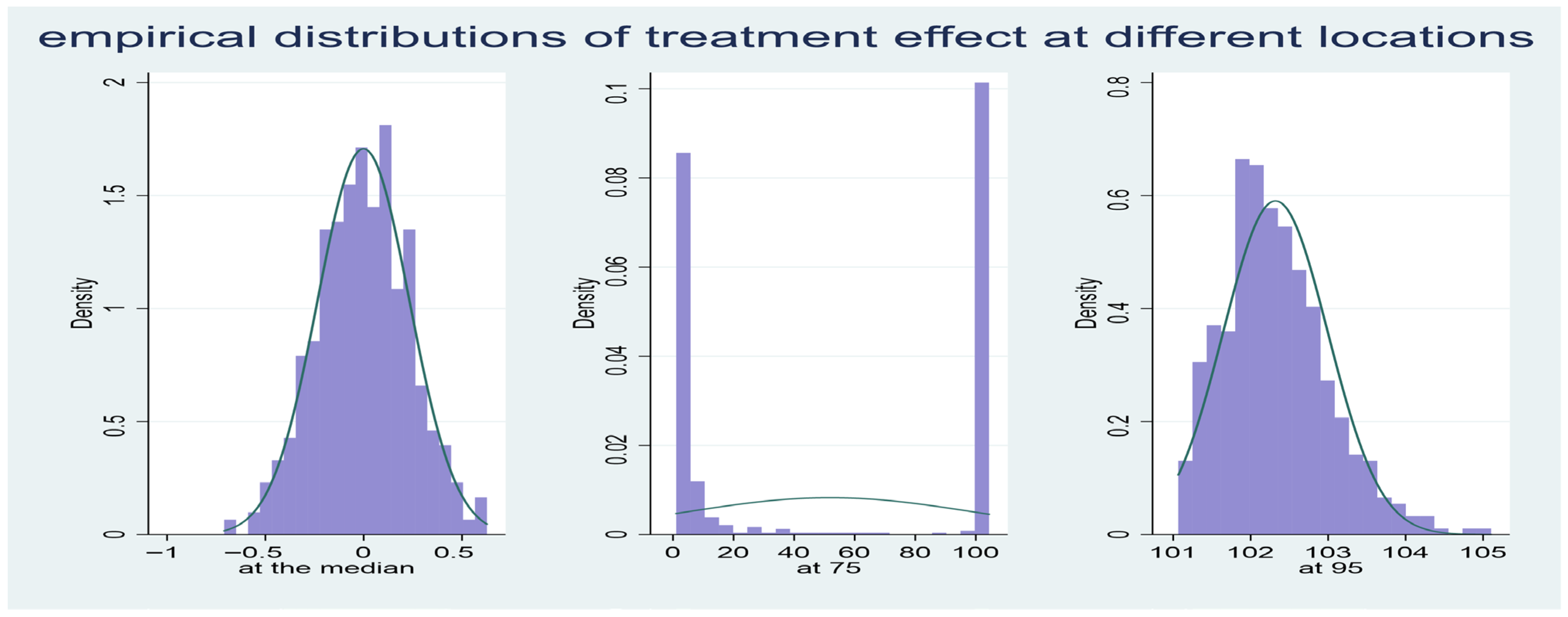
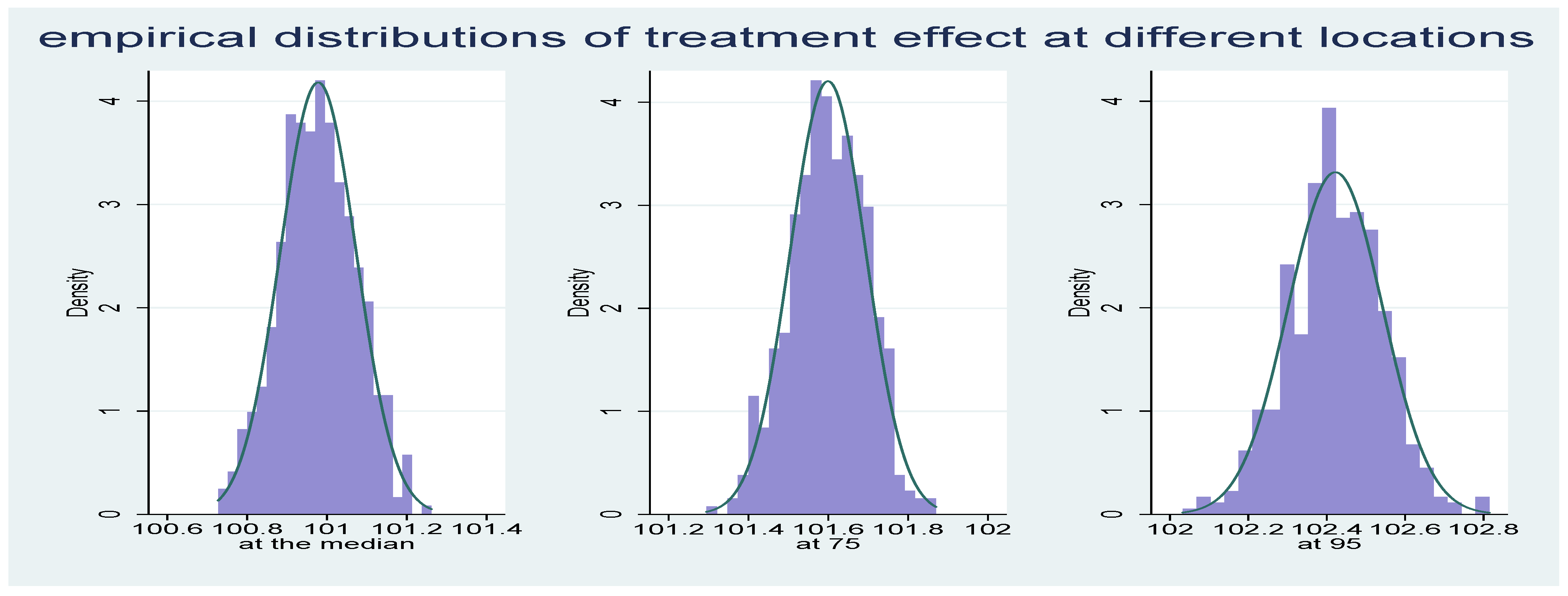
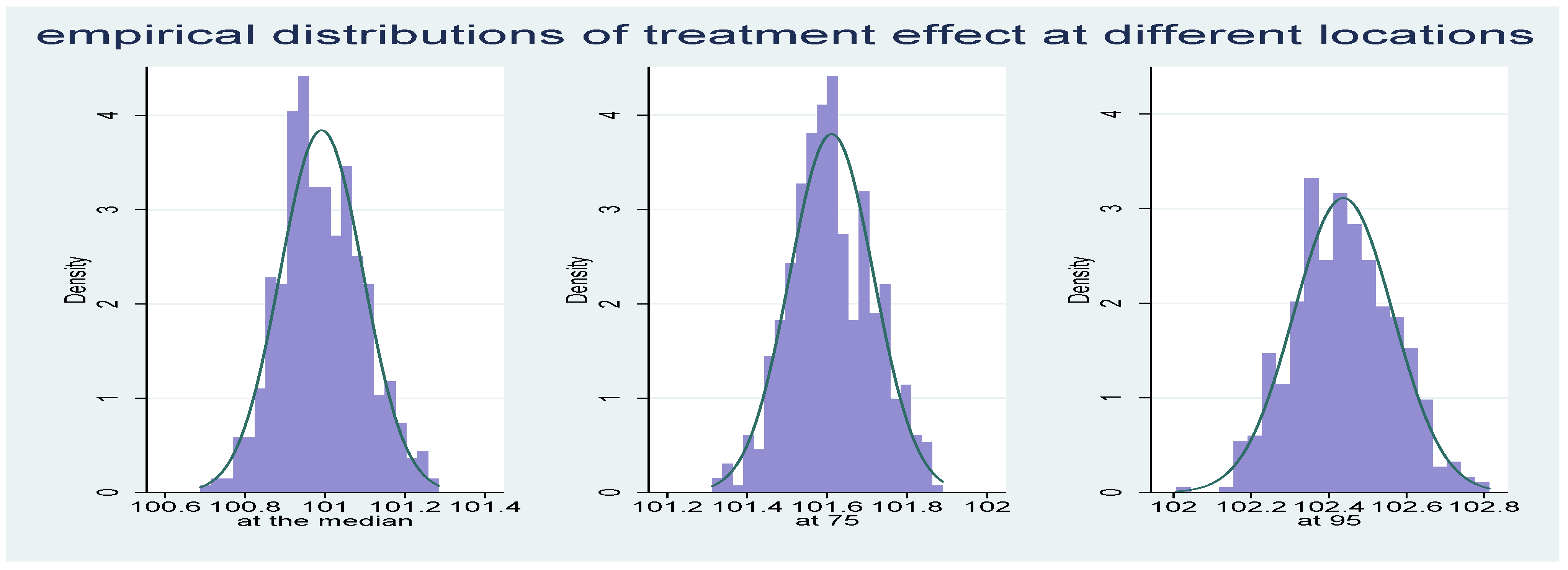
Figure 1, Figure 2 and Figure 3 collect the empirical distributions of the DR treatment effect estimates in the simulations. Figure 1 shows the DR empirical distributions when the probability of treatment is constant and follows a uniform distribution in the [0; 1] interval. At the median, it is bell-shaped and centered on zero, i.e., it does not capture the impact of treatment; at the 75th percentile, the graph shows a bimodal distribution with modes on zero and 100, implying that DR is missing the treatment effect in many iterations; finally, in the tail, DR provides a reliable measure of treatment, bell-shaped, centered on the true value, not too dispersed, and presenting a slight skewness.

The distributions in the other experiments, characterized by non-constant probability of treatment, present bell-shaped histograms with an increased dispersion in the far tail, at θ = 0.95.

Table 2. Summary statistics of the DR Estimated Treatment Effect at various locations: treatment effect equal to 100 involving 30% of the sample.

	50th	75th	95th
	Sample mean	Sample mean	Sample mean
True Treatment Effect	99.995	100.952	102.324
Standard deviation	(0.077)	(0.084)	(0.131)
Probability of treatment	Standard normal
Estimated Treatment Effect	−1.927	93.078	97.217
Standard deviation RMSE	St. dev. = 19.827 RMSE = 8.23	St. dev. = 20.270 RMSE = 10.75	St. dev. = 14.311 RMSE = 4.47
Probability of treatment	Contaminated normal
Estimated Treatment Effect	100.513	101.172	102.021
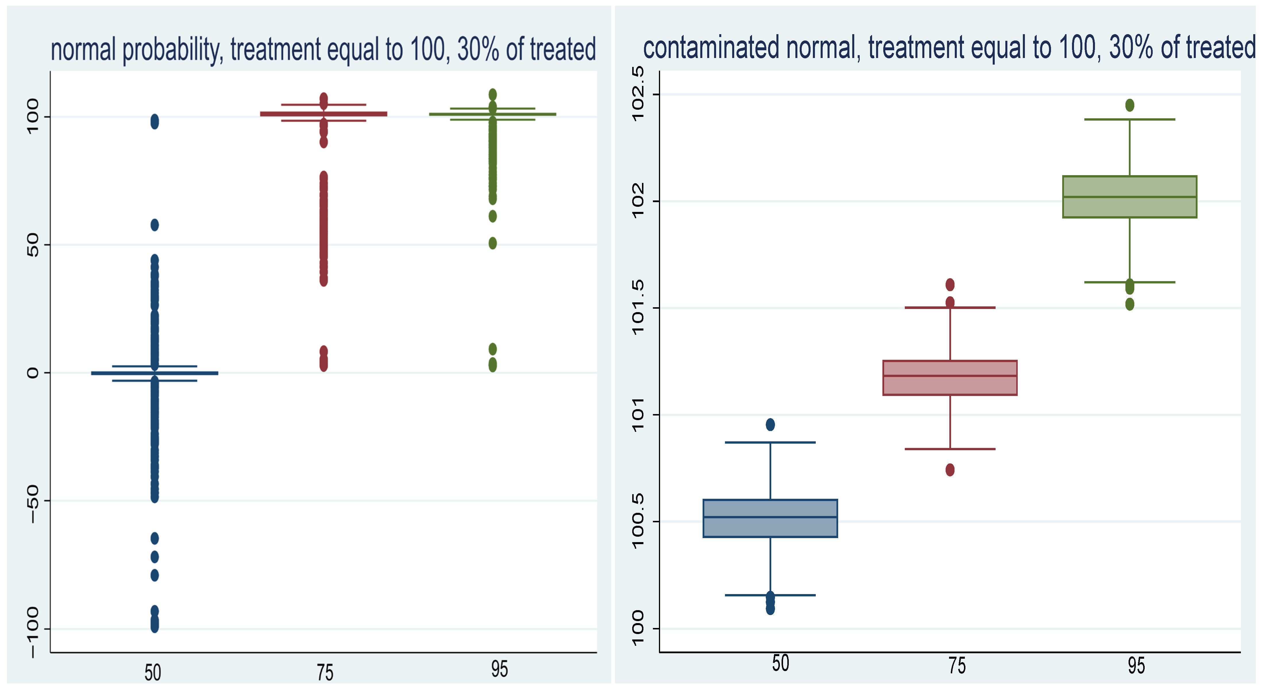
Standard deviation RMSE	St, dev. = 0.133 RMSE = 100.10	St. dev. = 0. 128 RMSE = 3.43	St. dev. = 0.141 RMSE = 0.66

collects the experiments when treatment involves a smaller percentage of the sample, 30%, and treatment has a mean equal to 100. We do not consider the case of constant probability of treatment, the uniform distribution, due to the poor performance of DR in the experiments reported in Table 1. When the probability of being treated follows a standard normal, DR is highly dispersed at all locations. It does not capture at all the treatment at the mean, possibly due to the reduced impact of treatment involving only 30% of the sample, while DR underestimates it at the 75th and 95th locations. The experiments with a contaminated normal probability of being treated, at the bottom of this table, show instead good performance in terms of both bias and dispersion. 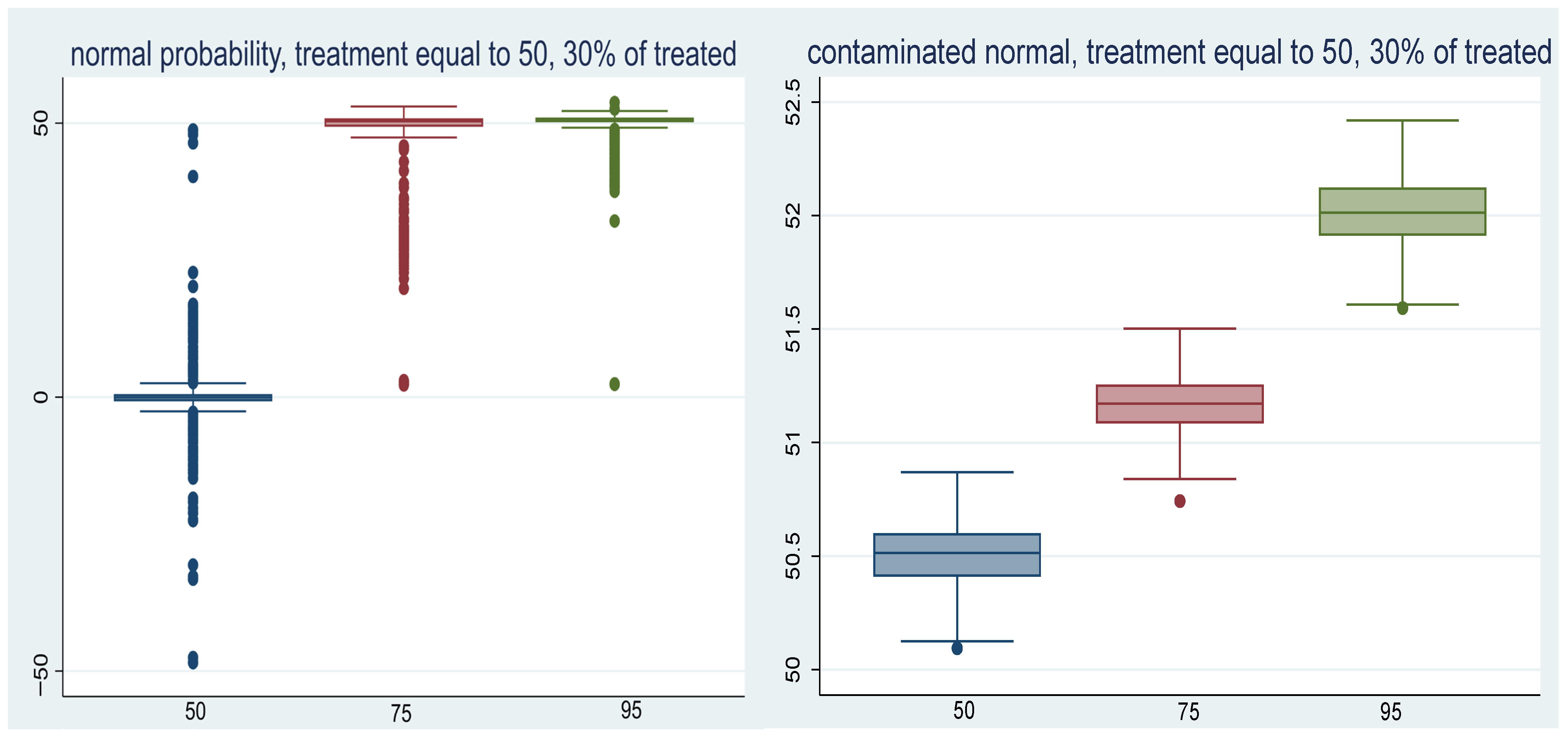Figure 4 reports the box plot of the DR empirical distributions, to the left when the probability of treatment is a standard normal and to the right when it follows a contaminated normal. The greater dispersion in the left-hand-side plots is quite evident compared with the good performance of the right-hand-side plots. At the mean, the box plot in the left graph does not capture treatment and is centered on zero.

Table 3. Summary statistics of the DR Estimated Treatment Effect at various locations: treatment effect equal to 50 involving 30% of the sample.

	50th	75th	95th
	Sample mean	Sample mean	Sample mean
True Treatment Effect	49.998	50.951	52.315
Standard deviation	(0.075)	(0.081)	(0.132)
Probability of treatment	Standard normal
Estimated Treatment Effect	0.216	46.742	49.396
Standard deviation RMSE	St. dev. = 9.295 RMSE = 4.08	St. dev. = 8. 744 RMSE = 4.72	St. dev. = 4.739 RMSE = 2.02
Probability of treatment	Contaminated normal
Estimated Treatment Effect	50.506	51.166	52.014
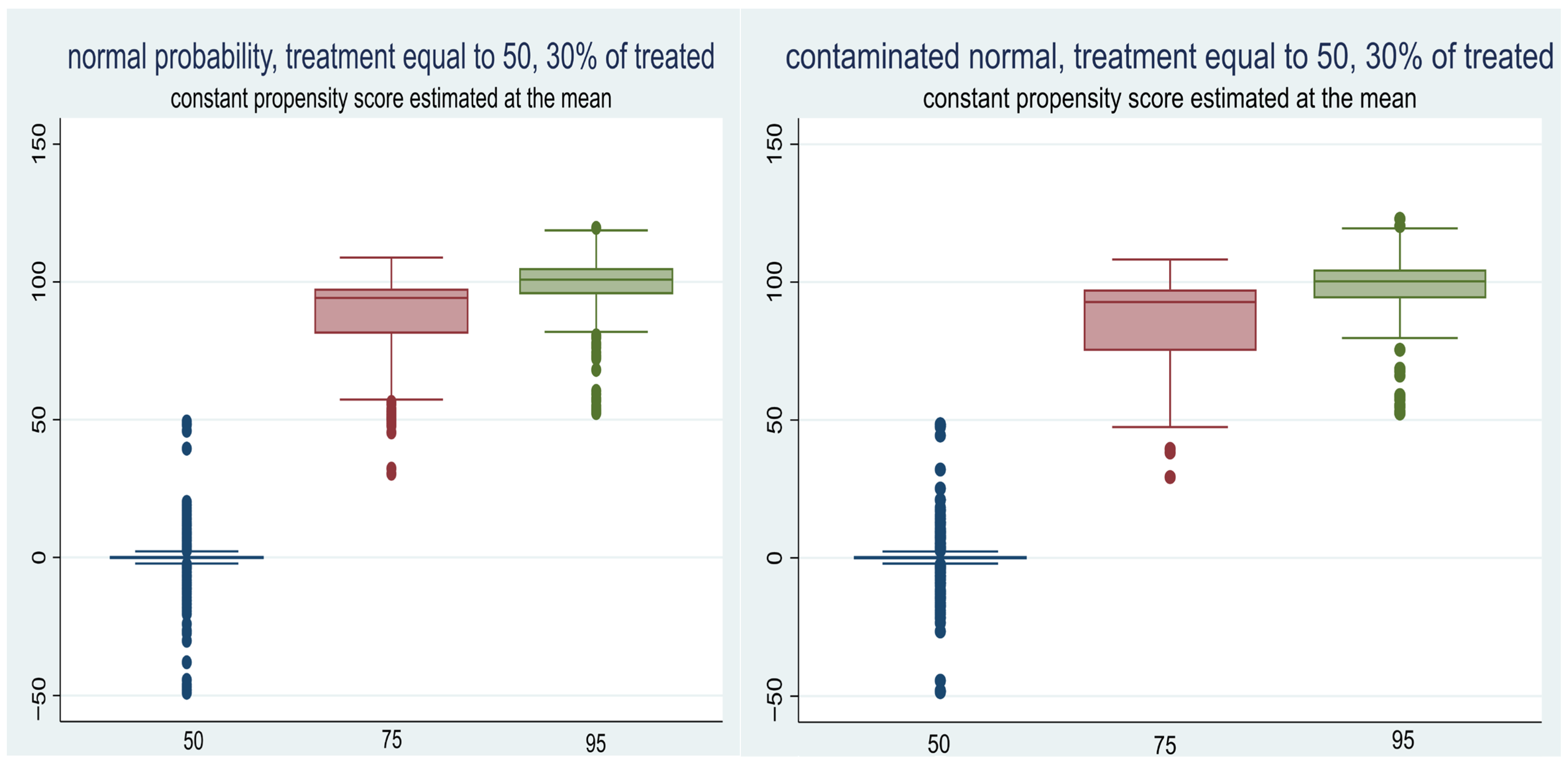
Standard deviation RMSE	St. dev. = 0.133 RMSE = 50.29	St. dev. = 0. 127 RMSE = 2.83	St. dev. = 0.143 RMSE = 0.65

reports the case of an even smaller treatment, where not only the percentage of treated but also its amount is reduced. 30% of the sample belongs to the treated group, and treatment has a mean equal to 50. When the probability of treatment is a standard normal, DR provides slightly underestimated results in the tail, at the 75th and the 95th locations, while it does not capture treatment at the mean. There is some dispersion, although it is less than the standard deviation values in the previous table for the same set of experiments, a standard normal probability of treatment. When the odds follow a contaminated distribution, DR has a good performance in terms of both bias and dispersion. Figure 5 reports to the left the box plot of the DR empirical distributions when the probability of treatment is a standard normal and to the right when it follows a contaminated normal. Once again, the greater dispersion in the plots to the left is quite evident compared to the right-hand-side plots.

Summarizing, we find that DR computed in the tails does not capture treatment if the probability of treatment is constant in the uniform distribution experiments. DR is a good estimator away from the mean when the probability of treatment is non-constant and symmetrical, following a standard normal. DR yields the best results at all locations when the probability of treatment is both non-constant and skewed, as in the contaminated normal.

The last table considers the case where only the regression component is measured in the tails, while the PS component is kept constant at the values estimated at the mean. The experiments consider a small treatment effect equal to 50, having an impact on only 30% of the sample. This is a counter example to see to what extent DR is reliable when the PS component does not move toward the tail.

Table 4. Summary statistics of the DR Estimated Treatment Effect at various locations, treatment effect equal to 50, involving 30% of the sample, changing PS unaccounted for and kept constant as estimated at the mean.

	50th	75th	95th
	Sample mean	Sample mean	Sample mean
True Treatment Effect	49.998	50.951	52.315
Standard deviation	(0.075)	(0.081)	(0.132)
Probability of treatment	Standard normal
Estimated Treatment Effect	−0.128	88.444	98.772
Standard deviation RMSE	St. dev. = 9.669 RMSE = 3.84	St. dev. = 14.172 RMSE = 40.37	St. dev. = 10.677 RMSE = 47.39
Probability of treatment	Contaminated normal
Estimated Treatment Effect	0.216	87.434	98.424
Standard deviation RMSE	St. dev. = 9.215 RMSE = 4.00	St. dev. = 13.870 RMSE = 39.43	St. dev. = 10.303 RMSE = 47.04

shows that treatment is not accounted for at the center, while it is overestimated at the 75th and 95th locations. The dispersion is quite sizable everywhere. This implies a tendency to overestimate the treatment effect in the tails if only the quantiles of the unconditional distributions are considered. When even PS is estimated in the tails, as occurs in the experiments of the previous tables, the overestimation tendency is balanced by the PS tail estimates. Figure 6 shows the great dispersion of empirical distributions in both sets of experiments, standard normal and contaminated normal probability of being treated. They are centered at zero at the mean and at values close to 100 for the 75th and 95th locations, thus significantly overshooting the target. When the probability of being treated is not constant, computing PS at the mean may possibly yield biased results.

5. Case Study

The Bank of Italy Survey of Household Income and Wealth data (SHIW) is analyzed, looking at the wave of 20208. The sample analyzes people aged 20–65, looking at their degree of education.

Table 5. Summary statistics, n = 15,298.

	Sample Mean	Standard Deviation
age	35.596	22.459
north	0.4368	0.4960
education	10.4821	4.742

collects the summary statistics of the variables of the model. Education is defined as the number of years needed to complete a degree. The PS component of DR considers the probability of completing higher education, beyond the required thirteen years of school, as the dependent variable. PS is estimated via logit and a weighted logit model—where the weights move the model away from the mean, toward the tails, as in (5). This probability is a function of age and age squared to non-linearly model ability and an additional variable causing group divergence. The source of heterogeneity between groups here considered is gender and, in turn, region of residence—capturing the negative impact of a lagging southern economy. Treated and untreated are compared on average and in the tails by DR, and

Table 6. Probability of higher education across gender, women versus men.

	50th		75th		95th
	coefficient		coefficient		coefficient
age	0.2096	(z = 22.99)	0.0564	(z = 18.87)	0.1074	(z = 24.00)
age square	−0.0024	(z = −22.26)	−0.0007	(z = −14.99)	−0.0013	(z = −23.31)
women	0.2261	(z = 4.72)	0.5760	(z = 1.46)	0.1203	(z = 4.73)
	50th		75th		95th
treatment effect	0.000	(se = 0.004)	4.224	(se = 0.104)	12.690	(se = 0.059)

DR difference in higher education, women versus men.

and

Table 7. Probability of higher education across regions, north versus the other regions.

	50th		75th		95th
	coefficient		coefficient		coefficient
age	0.2125	(z = 23.09)	0.0536	(z = 17.74)	0.1089	(z = 23.46)
age square	−0.0024	(z = −22.37)	−0.0007	(z = −14.09)	−0.0013	(z = −22.83)
north	0.3784	(z = 7.88)	0.1508	(z = 3.86)	0.2104	(z = 8.27)
	50th		75th		95th
treatment effect	0.116	(se = 0.042)	4.899	(se = 0.068)	13.519	(se = 0.060)

DR difference in higher education, north versus the other regions.

present the estimates of, respectively, gender and regional discrepancies. The first analysis considers gender as a possible source of disparity between groups. The top section of Table 6 reports the probability of higher education related to gender. The women’s coefficient is statistically significant and has an inverse u-shaped pattern, small at the center, increasing at 0.75, and declining at the top. Women have a great probability to continue education, significant throughout but at the 75th quartile.9 The bottom section of the table reports the DR estimated difference in education due to gender, which is non-significant at the center, small at 0.75, and increasing at 0.95, with the greatest gender difference in education at the top location. 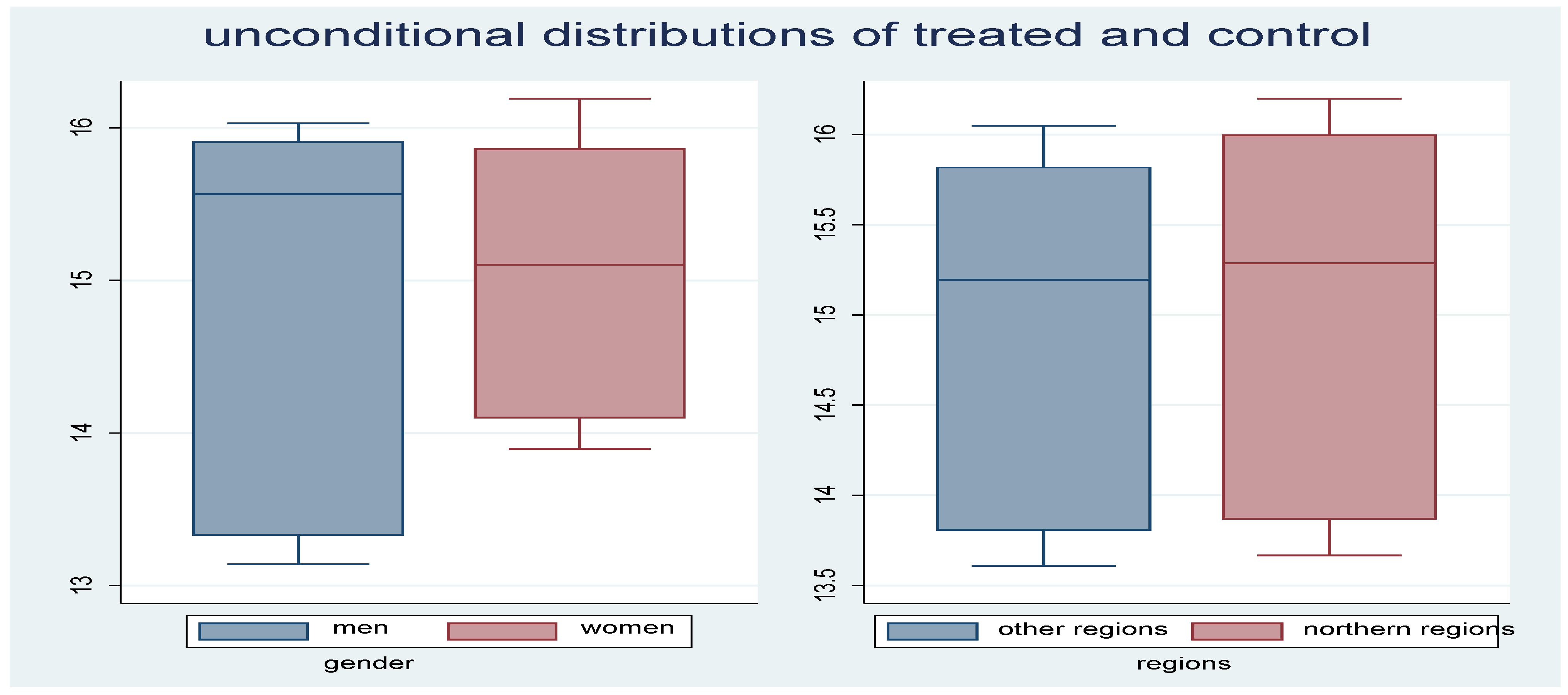While at the center, there is a non-significant difference in education between men and women; there is a larger number of highly educated women with respect to men at the top quantile.10 The left-hand side graph in Figure 7 depicts the unconditional distributions of treated and control in the gender analysis, and the unconditional distributions of education for men and women. The men’s plot is more dispersed. The presence of highly educated women, combined with their wider probability of attaining higher education, yields a positive and increasing DR difference at the selected locations. This finding can be related to Picchio and Mussida’s (2011) statement that women’s employment is higher in the right tail for highly educated women. Table 7 considers the difference in education across regions, comparing the north with all the other regions,11 where northern regions are economically more developed and provide better job opportunities. Living in the northern regions has a positive impact on the probability of studying, larger at the center, with a u-shaped pattern increasing in the tail, as reported in the top section of this table. The DR estimated difference in higher education is small but significant at the center and increases toward the tail. There is a prevalence of highly educated people residing in the northern regions. The right-hand side graph in Figure 7 depicts the unconditional distributions of treated and control in the regional analysis. The third quartile is higher in the northern region. The latter, combined with the positive impact of the regional variable on the probability of being treated, yields a positive double robust difference in higher education between regions, larger at the top location. This can be related to the significant internal migration within the country toward the northern regions, particularly for qualified workers, due to more favorable job market conditions in these economically more developed regions.

6. Additional Analysis: The Case of Mismatch

Next, we relax the constraint that sets the same location in both terms of the double robust estimator. The weights P(${\mathrm{w}}_{\mathrm{i}}{\mathrm{Z}}_{\mathrm{i}}=1|\mathbf{X}$) in the propensity score estimator, P(θ) in

Table 8. Relaxing the constraint of constant θ in both PS and regression quantile estimators. DR difference in attaining higher education, women versus men.

P(0.50) Q(0.25)		P(0.50) Q(0.75)		P(0.50) Q(0.95)		P(0.75) Q(0.25)		P (0.75) Q(0.95)		P(0.95) Q(0.25)		P(0.95) Q(0.75)
Coef.	se	Coef.	se	Coef.	se	Coef.	se	Coef.	se	Coef.	se	Coef.	se
−6.74	(0.061)	4.22	(0.085)	11.85	(0.114)	−6.48	(0.211)	11.45	(0.147)	−6.91	(0.088)	4.28	(0.092)

, are evaluated at locations that differ from the quantile of the difference Q in Equation (7), denoted Q(θ) in this table. Relaxing the requirement that propensity score and regression be evaluated at the same location may compromise the double robust property of this approach, since we combine estimates at different locations. However, the inequality of θ allows us to model interesting events. For instance, focusing on education with respect to gender, P(θ) is the probability of being highly educated, and Q(θ) is the quantile of education. The term P(0.75) Q(0.25) (looks at the high probability of higher education), P(0.75), associated with a lower educational attainment, Q(0.25). This entails looking at the unaccomplished probability of higher education, since the education quartile is rather low. Vice versa, P(0.50) Q(0.95) signals someone with a median probability of higher education achieving very high degrees of education. Having differences of θ in the double robust approach is a way to model mismatch, like highly educated people characterized by a low probability of higher education, P(0.50) Q(0.95), or vice versa, people unfulfilling their probability of higher education, P(0.95) Q(0.25). In Table 8, we compute the mismatch between probability and outcome distribution, comparing women versus men. All these estimates are statistically significant. In the first column, the negative sign of the estimate signals that women are unfulfilling, and the same occurs in the fourth and the sixth columns, when the degree of education Q(θ) is quite low with respect to the probability P(θ) of higher education. All the other columns present positive values, signaling women attaining higher education than their probabilities.

In this table, coefficients that differ significantly from the values in the bottom section of Table 6 are highlighted in bold. Most of the results in Table 8 are outside the $\mp$2$\hat{\mathsf{\sigma }}$ confidence interval of the estimates in Table 6, with only one exception of P(0.50) Q(0.75). Thus, gender has a significant impact on attaining higher education, even if the probability of higher education is not very large. Women achieve higher education at rates exceeding their probabilities in greater numbers.

Finally, the estimates in Table 8—characterized by differing θ—can also be interpreted as a sort of confidence interval of the values in the previous section of the table—computed by constraining the same θ in both components of DR. For instance, P(0.25) Q(0.50) and P(0.75) Q(0.50) could be considered, respectively, as the lower and the upper bound of Q(0.50).

7. Conclusions

In this study, we allow propensity scores to be non-constant and estimate treatment probability at and away from the mean. The focus is on the probability of being treated in the tails to consider the double robust estimator as computed beyond average for both components of this estimator, the propensity score and the regression model. In previous studies, we focused exclusively on the regression component estimated away from the mean.

The Monte Carlo study shows that with a constant probability of being treated, there is not really a need to implement the double robust estimator in the tails.

This conclusion changes if the probability of treatment is non-constant, and more so when the changing probability is skewed. In the presence of a standard normal or of a contaminated normal probability of treatment, it is advisable to implement the double robust estimator discussed here and compute treatment odds in the tail. A final experiment, where changing probability is not accounted for, shows the tendency of quantile regression estimates to overshoot the target. Vice versa, when the changing probability is accounted for, the overestimation of the regression component is balanced by the propensity score tail estimates, yielding results closer to the target.

A case study considers Italian data on education from the Banca d’Italia Survey of Household Income and Wealth in the year 2020. Gender and, in turn, region of residence are considered as causes of group heterogeneity in completing higher education. The results show that women and, in turn, people living in the northern regions attain higher education. Women fulfill their probabilities of higher education more than men, and people in the northern regions more than people residing in the other regions. Next, a mismatch between the location of the propensity score and outcome allows us to model a mismatch between probability and attainment—in this example, between the probability of higher education and the degree of education across gender. In the case study here analyzed, women attain higher education at rates exceeding their probabilities: gender has a significant impact on attaining higher education, even if the probability of higher education is not very large.

Further analysis could consider the relaxed double robust estimator (Xu & Zhao, 2024). The introduction of an eased requirement for double robustness is an interesting approach to be implemented within the quantile regression setting. The study would benefit from further investigation comparing the proposed method with other double robust and quantile regression-based approaches, like the efficient influence function or the marginal structural quantile model. This would point out the comparative advantages and drawbacks of the proposed method. Multiple treatments could also be a relevant extension. These ideas are left to future research.