Nonparametric Autoregressive Copula Forecasting via Boundary-Reflected Kernel Estimation

Abstract

We propose a fully nonparametric empirical autoregressive copula framework for univariate time series, designed to capture nonlinear and asymmetric serial dependence while exactly preserving the empirical marginal distribution. The method decouples marginal behavior from temporal dependence by (i) constructing a shape-preserving empirical marginal via monotone interpolation and mapping observations to the unit interval, and (ii) estimating the lag–lead dependence through a nonparametric conditional AR(1) copula density on ${(0,1)}^2$. To ensure stable estimation near the boundaries, we employ reflection-based kernel methods that mitigate edge effects and yield well-behaved conditional densities on the unit support. Forecasts are obtained from the implied conditional predictive density: we compute point forecasts either as conditional modes (maximum a posteriori) on the copula scale or as conditional means, and then back-transform exactly using the empirical quantile function, guaranteeing marginal fidelity and support-respecting predictions. Empirically, we evaluate the approach on three CBOE volatility indices (VIX, VXD, and RVX) and benchmark it against linear ARMA models, copula-based parametric competitors, and state-space/heteroskedasticity baselines (Local level, TVP–AR, and ARMA–GARCH). The results highlight that modeling the full conditional transition density nonparametrically can deliver competitive—often best or near-best—forecast accuracy across horizons, particularly in the presence of pronounced volatility regimes and asymmetric adjustments.

1. Introduction

Modeling nonlinear autoregressive dependence is a fundamental problem in time series analysis, particularly when the underlying dynamics depart from linear or moment-based representations. Many commonly used approaches impose restrictive parametric structures on temporal dependence and characterize dynamics through a limited set of summary features, such as conditional moments. While effective in specific settings, these formulations offer limited flexibility to accommodate nonlinear, asymmetric, and state-dependent autoregressive relationships. Copula-based methods provide a natural alternative by separating marginal behavior from serial dependence, thereby allowing nonlinear autoregressive structures to be modeled directly and in a probabilistically coherent manner. This perspective is especially appealing in applications where complex dependence patterns arise naturally, such as in volatility dynamics.

Copula-based models formalize this separation by decoupling marginal distributions from the serial dependence structure, thereby enabling a flexible representation of temporal dependence that is not tied to specific moment conditions. This framework allows both serial and cross-sectional dependence to be modeled directly, accommodating nonlinear, asymmetric, and non-monotonic dependence patterns, including tail dependence, within a coherent probabilistic setting (Nelsen, 2007; Patton, 2006, 2012). As a result, copulas have become a central tool for modeling complex dependence structures in time series and multivariate data. In applied contexts such as volatility modeling, this flexibility proves particularly valuable for reproducing empirically observed features including persistence, heavy tails, and asymmetric dependence (McNeil, 2021). These characteristics are well documented in realized volatility and realized variance measures derived from high-frequency data, which exhibit strong persistence, non-Gaussian distributions, and pronounced tail behavior (Andersen et al., 2003; Barndorff-Nielsen & Shephard, 2002, 2004).

Seminal contributions include Patton (2006), who modeled exchange-rate dependence with time-varying copulas and documented stronger correlations during depreciations, and Ning et al. (2008), who demonstrated nonlinear, time-varying leverage effects in the relation between returns and realized volatility. Building on these ideas, Sokolinskiy and van Dijk (2011) proposed an autoregressive copula to forecast realized volatility, while subsequent studies extended autoregressive dependence to multivariate settings via vine copulas (Aas, 2016; Brechmann & Czado, 2015; Czado et al., 2019). More recently, McNeil (2021) incorporated ARMA-type dynamics into copulas to capture volatility clustering and heavy tails, and Nankali et al. (2025) introduced dynamic copula networks to model high-dimensional dependence.

Recent advances have also explored conditional copula structures in dynamic settings. For example, Nankali et al. (2025) proposed dynamic copula networks combined with quantile regression for volatility forecasting, while Jobst et al. (2024) developed conditional vine copulas whose parameters vary with covariates through gradient boosting. These methods expand the literature, but generally rely on parametric or semiparametric specifications rather than fully empirical estimation of the conditional dependence structure.

In parallel, a growing body of literature has studied nonparametric copula estimation. Lu and Ghosh (2021) introduced the Empirical Checkerboard Bernstein Copula (ECBC), which yields smoothed multivariate copula estimates with strong asymptotic guarantees and ensures valid copula properties even in finite samples. Related advances in nonparametric density estimation, though not specific to copulas, are directly relevant to our empirical setup because both the uniformized marginals and the copula live on compact supports and suffer from edge effects. For example, Yang (2023) develops exact boundary-correction methods for multivariate Kernel Density Estimator (KDE) on compact supports, and Cattaneo et al. (2023) proposes boundary-adaptive local polynomial conditional density estimators. These results show classical challenges, boundary bias, bandwidth selection, and the smoothness–variance trade-off, and motivate our design choices: boundary-reflected KDE for the conditional copula density, coupled with monotone interpolation for the marginals, to mitigate edge bias without imposing parametric structure.

Realized volatility dynamics (Andersen et al., 2003; Barndorff-Nielsen & Shephard, 2002, 2004) provide a convenient and empirically relevant setting for studying nonlinear autoregressive dependence through conditional density modeling. Volatility series are characterized by strong persistence, heavy-tailed and asymmetric marginal distributions, and state-dependent responses to shocks. These features generate complex transition dynamics that are often difficult to represent within parametric autoregressive frameworks formulated solely in terms of conditional moments. In particular, volatility distributions tend to deviate substantially from Gaussianity, which complicates the joint specification of marginal behavior and temporal dependence within a single parametric model.

Observed volatility proxies such as the VIX pose a particularly challenging modeling problem. Their marginal distributions are typically highly skewed and heavy-tailed, contaminated with measurement errors, with sharp upper support driven by market stress episodes. At the same time, volatility dynamics exhibit strong persistence combined with pronounced state dependence: conditional behavior following low-volatility regimes differs markedly from that observed during high-volatility periods. In addition, the adjustment dynamics of volatility are often asymmetric and nonlinear, with large upward movements clustering differently from subsequent downward corrections. Capturing these features jointly within conventional parametric autoregressive models can therefore be challenging, particularly when the dependence structure itself varies across states of the process.

Traditional volatility models approach this problem from a different perspective. A large body of the financial econometrics literature models volatility as a latent process inferred from asset returns. Prominent examples include GARCH-type models and stochastic volatility specifications, which treat volatility as an unobserved state variable whose dynamics are estimated through parametric assumptions on the return-generating process and the evolution of conditional variance. These frameworks have proven highly successful in capturing key stylized facts of financial time series, including volatility clustering, persistence, and asymmetric responses to shocks, and they play a central role in applications such as volatility forecasting, portfolio allocation, and risk management.

When the object of interest is an observed volatility proxy, such as implied volatility indices or realized volatility measures, the modeling perspective differs somewhat. In these cases, the empirical objective is to describe the dynamics of an observable volatility series rather than to infer an unobserved volatility component from returns. Latent volatility models can still be applied in this setting, although the resulting specification effectively characterizes the dynamics implied by the chosen parametric volatility process. While such approaches remain informative, they may not fully exploit the empirical transition structure directly observable in volatility proxies themselves.

Copula-based autoregressive models provide an alternative and complementary perspective by modeling the conditional distribution of the observed volatility series directly. Within this framework, marginal distributions and serial dependence are specified separately, which allows greater flexibility in accommodating non-Gaussian marginals and nonlinear state-dependent dynamics. Parametric copula autoregressive models already represent an important step in this direction, although their ability to capture complex dependence patterns may still be constrained by the choice of a specific parametric copula family. These considerations motivate the use of a more flexible nonparametric copula framework capable of accommodating richer forms of dependence in volatility dynamics.

These features motivate a modeling strategy centered on the estimation of conditional densities rather than conditional moments. An empirical copula-based framework is well suited for this purpose, as it separates marginal behavior from serial dependence and enables the construction of a conditional transition density on a standardized uniform scale. After uniformization via the empirical distribution function, the autoregressive dynamics are fully characterized by the joint density of consecutive states and the associated conditional density of the next observation given the current state. Forecasting can then be formulated as the evaluation of functionals of this conditional density—such as its mode or conditional mean—which naturally accommodates nonlinear, asymmetric, and state-dependent dependence structures.

Against this background, the objective of this paper is to develop a fully empirical copula-based framework for modeling nonlinear autoregressive dependence in time series through direct estimation of the conditional transition density. Rather than specifying parametric dynamics for conditional moments or imposing functional forms on the dependence structure, the proposed approach estimates the conditional distribution of the next observation given the current state using nonparametric methods on the copula scale. By combining empirical marginal transformations with a boundary-corrected kernel estimator of the conditional copula density, the framework provides a flexible and data-driven representation of temporal dependence that accommodates nonlinear, asymmetric, and state-dependent dynamics while preserving the probabilistic coherence of copula models.

Our approach differs in key respects from existing nonparametric copula methods. We combine empirical marginals obtained via monotone interpolation with a conditional autoregressive copula estimated nonparametrically using kernel density estimation with boundary reflection. This design preserves the empirical marginal distribution, mitigates boundary bias on the unit support, and yields a well-defined conditional density that can be used to construct one-step-ahead forecasts via both maximum a posteriori (MAP) and conditional mean predictors. In contrast to approaches such as the Empirical Checkerboard Bernstein Copula and related methods, our focus is explicitly on modeling serial dependence and generating forecasts in a time-series setting.

Within this framework, the marginal distribution enters exclusively via the probability integral transform and its inverse, while all aspects of temporal dependence are captured by the conditional copula density on the uniform scale. This separation enables the autoregressive transition density to be estimated fully nonparametrically, without imposing parametric assumptions on either the marginal distribution or the dependence structure. In the empirical analysis, we analyzed volatility indices to demonstrate how the proposed model captures nonlinear temporal dependence and produces forecasts directly from the estimated conditional density, rather than relying on moment-based recursions.

Although the empirical application focuses on the realized volatility, the proposed framework is not specific to volatility modeling. Any univariate time series characterized by bounded support, heavy-tailed marginals, or nonlinear state-dependent dynamics—such as interest rate spreads, climate indices, risk measures, or transformed macroeconomic indicators—can be naturally accommodated within the same empirical copula-based autoregressive structure.

This paper makes three main contributions. First, it proposes an empirical copula-based autoregressive framework that separates marginal estimation from the nonparametric estimation of the serial dependence structure, allowing the transition density of the process to be recovered without imposing parametric restrictions. Second, it develops a practical estimation strategy that combines monotone interpolation for the marginals with boundary-reflected kernel density estimation for the conditional copula density, addressing well-known boundary issues on compact supports while preserving the empirical distribution. Third, it shows how forecasts can be constructed directly from the estimated conditional density, providing a flexible alternative to moment-based forecasting methods commonly used in volatility modeling.

2. Model

We develop an empirical autoregressive copula framework for modeling the conditional dynamics of a univariate time series while preserving full flexibility in both the marginal distribution and the dependence structure. The central idea is to represent temporal dependence through the copula linking consecutive observations, while estimating the marginal distribution nonparametrically. This separation allows the conditional transition density of the process to be learned directly from the data without imposing restrictive parametric assumptions.

Our contribution is threefold. First, we construct a smooth empirical marginal distribution using a shape-preserving interpolation scheme based on the Piecewise Cubic Hermite Interpolating Polynomial (PCHIP). This approach provides a monotone and numerically stable representation of both the distribution function and its inverse, allowing observations to be mapped to the unit interval while preserving the empirical structure of the sample.

Second, we estimate the lag–lead copula density nonparametrically using kernel density estimation on the unit square combined with a reflection-based correction to mitigate boundary bias. This produces a smooth empirical copula density capable of capturing nonlinear, asymmetric, and state-dependent dependence patterns that are difficult to represent with standard parametric copula families.

Third, the estimated copula density is used to construct forecasting operators directly on the uniform scale. In particular, we derive both a maximum a posteriori (MAP) predictor and a conditional-mean predictor, which are then mapped back to the original data scale through the estimated quantile function. This representation yields a flexible and fully data-driven autoregressive forecasting mechanism based on the estimated transition density.

As shown in Nelsen (2007), a copula is a function that separates the dependence structure from the marginal behavior of a joint distribution. For a pair $(X,Y)$ with marginal distribution functions $F\left(x\right)=P(X\le x)$ and $G\left(y\right)=P(Y\le y)$ and joint distribution $H(x,y)=P(X\le x,Y\le y)$, there exists a function $C:{[0,1]}^2\to [0,1]$, the copula, such that

$$H(x,y)=C\left(F\left(x\right),G\left(y\right)\right).$$

Equivalently, if $U=F\left(X\right)$ and $V=G\left(Y\right)$, then $U,V\sim \mathrm{U}(0,1)$ and the copula is their joint distribution,

$$C(u,v)=P(U\le u,V\le v).$$

Thus, F and G encode the univariate margins, while C captures all aspects of dependence (asymmetry, tail behavior, etc.). This decomposition, formalized by Sklar’s theorem (Nelsen, 2007), allows margins and dependence to be modeled modularly.

In an autoregressive copula structure for a univariate series, we build the copula to account for temporal dependence:

$$H(x_t,x_{t-1})=C\left(F\left(x_t\right),F\left(x_{t-1}\right)\right).$$

Let $\mathcal{X}={\left\{x_t\right\}}_{t=1}^T$ denote the training sample. Sort it as $x_{\left(1\right)}\le \dots \le x_{\left(T\right)}$ and assign central ranks

$$u_{\left(t\right)}={\displaystyle \frac{t-\frac{1}{2}}{T}},t=1,\dots ,T.$$

(1)

To ensure strict monotonicity for interpolation, we collapse ties. Let ${\left\{x_k^{*}\right\}}_{k=1}^{T_{\mathrm{eff}}}$ be the strictly increasing set of unique values and, for each tie block $B_k=\{t:x_{\left(t\right)}=x_k^{*}\}$ corresponding to all values in the sample with the same x, define the averaged rank

$$u_k^{*}={\displaystyle \frac{1}{|B_k|}}\sum _{t\in B_k}{u}_{\left(t\right)},k=1,\dots ,T_{\mathrm{eff}}.$$

(2)

We use a small, data-dependent boundary cushion

$$\epsilon ={\displaystyle \frac{1}{10T_{\mathrm{eff}}}},u_{min}=\epsilon ,u_{max}=1-\epsilon ,$$

(3)

and denote $x_{min}=x_1^{*}$, $x_{max}=x_{T_{\mathrm{eff}}}^{*}$.

Collapsing ties ensures that the pairs $(x_k^{*},u_k^{*})$ are strictly increasing, which is required for the construction of a monotone interpolant. The small boundary cushion keeps the transformed values away from the endpoints of the unit interval. In finite samples, empirical ranks may approach the boundaries of $[0,1]$, which can lead to numerical instability when evaluating kernel densities or conditional ratios near the edges of the copula domain. The cushion parameter $\epsilon$ therefore restricts the effective support of the transformation to the open interval $(u_{min},u_{max})=(\epsilon ,1-\epsilon )$. The choice $\epsilon =1/\left(10T_{\mathrm{eff}}\right)$ provides a small, sample-size-dependent offset that vanishes asymptotically as the sample size increases, while ensuring stable interpolation and density evaluation in finite samples. The corresponding bounds $x_{min}$ and $x_{max}$ denote the smallest and largest observed values in the strictly increasing sample.

The empirical distribution function provides a nonparametric representation of the marginal distribution, but it is defined as a step function on the observed sample. For the purposes of the copula construction and the forecasting procedure, we require smooth evaluations of both the cumulative distribution function and its inverse, since observations must be mapped continuously between the original scale and the unit interval. Direct inversion of the empirical distribution would lead to a piecewise-constant transformation, which may generate numerical instability and discontinuities when computing conditional densities or iterating forecasts. To address this issue, we construct a smooth monotone interpolant that approximates the empirical distribution while preserving its ordering structure.

With the pairs $\left\{(x_k^{*},u_k^{*})\right\}$ we build a shape-preserving interpolator through Piecewise Cubic Hermite Interpolating Polynomial (PCHIP), as in Fritsch and Butland (1984), for the CDF and its inverse (quantile function). The interpolant preserves monotonicity and avoids overshooting:

$$\begin{array}{cc}\hfill \widehat{F}\left(x\right)& \approx \mathrm{PCHIP}\left(\left\{x_k^{*}\right\},\left\{u_k^{*}\right\}\right)\left(x\right),\hfill \end{array}$$

(4)

$$\begin{array}{cc}\hfill {\widehat{F}}^{-1}\left(u\right)& \approx \mathrm{PCHIP}\left(\left\{u_k^{*}\right\},\left\{x_k^{*}\right\}\right)\left(u\right).\hfill \end{array}$$

(5)

We then define

$$\begin{array}{cc}\hfill \mathrm{cdf}\left(x\right)& =\widehat{F}\left(x\right),\hfill \end{array}$$

(6)

$$\begin{array}{cc}\hfill \mathrm{ppf}\left(u\right)& ={\widehat{F}}^{-1}\left(u\right).\hfill \end{array}$$

(7)

The marginal transformation in the model is $u=\mathrm{cdf}\left(x\right)\in (u_{min},u_{max})$ with inverse $x=\mathrm{ppf}\left(u\right)\in [x_{min},x_{max}]$. Thus, heavy tails and skewness are handled by $\widehat{F}$, while temporal dependence is modeled on the uniform scale.

After mapping the observations to the uniform scale through $x_t\mapsto u_t=\widehat{F}\left(x_t\right)$, the dependence structure of the process is fully characterized by the joint distribution of the lag–lead pairs $(U_{t-1},U_t)$. A purely empirical copula constructed from the sample would place probability mass only on the observed points, resulting in a discrete representation that is not suitable for evaluating conditional densities or generating forecasts. In particular, forecasting requires a smooth estimate of the transition density that assigns probability mass to regions of the unit square that may not be directly observed in the sample. To obtain such a representation, we estimate the copula density using kernel density estimation (KDE), which smooths the sample points and provides a flexible nonparametric approximation of the underlying density on ${[0,1]}^d$. For this purpose, we use the Gaussian KDE

$${\widehat{f}}_U\left(u\right)={\displaystyle \frac{1}{n_{\mathrm{aug}}{h}^d}}\sum _{j=1}^{n_{\mathrm{aug}}}\phi \left({\displaystyle \frac{u-{\tilde{u}}_j}{h}}\right),\phi \left(z\right)={\displaystyle \frac{1}{{\left(2\pi \right)}^{d/2}}}{e}^{-\frac{1}{2}{\parallel z\parallel }^2},$$

where d is the data dimension. The bandwidth h controls the degree of smoothing: small h yields a rough estimate, large h oversmooths the density.

In our time-series application, the bivariate sample consists of lag–lead pairs $(u_{t-1},u_t)$, so the effective sample size is $n=T-1$ for the joint estimator, and the reflected sample size is denoted by $n_{\mathrm{aug}}$ after augmentation. The data dimension is $d=2$ for the joint KDE and $d=1$ for the marginal KDE used in the conditional ratio.

h is selected according to Scott’s rule (Scott, 1992), given by

$$h=n^{-\frac{1}{d+4}},$$

so that the effective kernel covariance is $h^2\Sigma$, with $\Sigma$ the sample covariance of the data. This rule adapts to sample size n and dimension d, shrinking h as more data become available. Estimating the optimal bandwidth h via cross-validation could improve the fit, albeit at a higher computational cost.

This estimator places Gaussian weights around each observation to construct a smooth surface for the copula density. However, since the Gaussian kernel is supported on the real line $\mathbb{R}$, when the data lie near the boundaries of ${[0,1]}^2$, part of the kernel mass is spread outside the copula domain. This generates boundary bias: the density near the edges is underestimated because probability mass leaks outside the unit square.

Because the copula density is defined on the bounded support ${[0,1]}^d$, standard kernel density estimators suffer from boundary bias near the edges of the domain. In particular, kernels such as the Gaussian kernel have unbounded support on ${\mathbb{R}}^d$, so when observations lie close to the boundaries of the unit interval, a portion of the kernel mass is assigned outside the admissible region. As a result, the density estimator systematically underestimates the true density near the boundaries, since probability mass that should contribute to the estimate inside the domain effectively “leaks” outside the support.

To mitigate this issue, we adopt a reflection scheme at the boundaries of the unit interval. Concretely, each observation $u_i$ is augmented with reflected counterparts across the boundaries at 0 and 1; for example, $-u_i$ and $2-u_i$. The kernel density estimator is then evaluated only within the admissible region $[0,1]$, so that the reflected observations reinject the probability mass that would otherwise fall outside the support. Intuitively, the reflected points act as mirror images of the original observations near the boundary, ensuring that the smoothing procedure remains symmetric and that the total probability mass is preserved within the domain.

Reflection-based correction is widely used in nonparametric density estimation on bounded domains because it provides a simple and computationally efficient way to reduce boundary bias while retaining the desirable properties of standard kernels (Fernandes & Monteiro, 2005; Jones, 1993; Schuster, 1985). In contrast to alternative approaches, such as boundary kernels or transformations of the support, the reflection method preserves the shape and bandwidth structure of the original kernel estimator and integrates naturally with the Gaussian KDE used in our copula density estimation. This makes it particularly convenient in the present setting, where the support of the copula is naturally bounded by the unit square.

In the bivariate case $(u_{t-1},u_t)\in {[0,1]}^2$, the same idea is applied component-wise, yielding an augmented set of reflected pairs used to fit the joint KDE.

$$\tilde{\mathcal{U}}=\left\{u_i\right\}\cup \{-u_i\}\cup \{2-u_i\},$$

keeping only the reflected points that remain inside $[0,1]$. This effectively reinjects the density that otherwise would fall outside the copula back into its domain, correcting for the boundary bias (Muia et al., 2025). With this adjustment, the KDE ${\widehat{f}}_U\left(u\right)$ can be safely employed to estimate the empirical copula density, even close to the borders of the unit square.

Temporal dependence is captured by the copula of $(U_{t-1},U_t)$. The conditional density is

$${\widehat{f}}_{U_t\mid U_{t-1}}(v\mid u)={\displaystyle \frac{{\widehat{f}}_{U_{t-1},U_t}(u,v)}{{\widehat{f}}_{U_{t-1}}\left(u\right)}}.$$

(8)

Since ${\widehat{f}}_{U_{t-1}}\left(u\right)$ does not depend on v, maximizing the conditional density ${\widehat{f}}_{U_t\mid U_{t-1}}(v\mid u)$ is equivalent to maximizing the joint density ${\widehat{f}}_{U_{t-1},U_t}(u,v)$ with respect to v for fixed u.

Once the joint density of the lag–lead pair $(U_{t-1},U_t)$ has been estimated, it naturally induces a predictive distribution for the next observation. In the copula framework, forecasting amounts to characterizing the conditional distribution of $U_t$ given the current state $U_{t-1}=u$. The estimated joint density ${\widehat{f}}_{U_{t-1},U_t}(u,v)$ therefore provides a nonparametric approximation to the transition density of the latent uniform process. From this conditional distribution, different point forecasts can be derived depending on the loss function used to evaluate forecast accuracy (Robert, 2007).

The first approach is based on the maximum a posteriori (MAP) principle (Robert, 2007), which selects the value of v that maximizes the conditional density. This predictor identifies the most probable next state under the estimated transition density and can be interpreted as the optimal forecast under a zero–one loss defined on small neighborhoods of the state space. The MAP forecast is particularly informative when the conditional distribution is asymmetric or multimodal, situations that frequently arise in volatility dynamics.

A second approach considers the conditional mean of the future observation, which corresponds to the optimal predictor under quadratic loss and is therefore directly aligned with standard forecast evaluation metrics such as mean squared error (MSE). Because the dependence structure is modeled on the copula scale while the observed variable lives on the original scale, the conditional expectation must be computed by integrating the empirical quantile function against the estimated joint density.

These two forecasting rules provide complementary summaries of the predictive distribution. The MAP predictor emphasizes the most likely transition in the latent uniform space, while the conditional-mean predictor aggregates information across the entire predictive distribution and produces forecasts directly on the original data scale.

The one-step maximum a posteriori (MAP) predictor selects

$${\widehat{u}}_t^{\mathrm{MAP}}\left(u\right)\in arg\underset{v\in (0,1)}{max}{\widehat{f}}_{U_{t-1},U_t}(u,v),$$

(9)

implemented numerically on a uniform grid $g={\left\{g_{\ell }\right\}}_{\ell =1}^G\subset (0,1)$. Since ${\widehat{f}}_{U_{t-1}}\left(u\right)$ does not depend on v, maximizing the conditional density ${\widehat{f}}_{U_t\mid U_{t-1}}(v\mid u)$ is equivalent to maximizing the joint density ${\widehat{f}}_{U_{t-1},U_t}(u,v)$ with respect to v for fixed u.

In addition to the MAP predictor, we also consider a conditional-mean forecast on the original scale. Let $q\left(v\right)={\widehat{F}}^{-1}\left(v\right)$ denote the empirical quantile function. Using the smoothed joint density on ${[0,1]}^2$, we compute

$${\widehat{x}}_t^{\mathrm{mean}}\left(u\right)=\mathbb{E}[X_t\mid U_{t-1}=u]\approx {\displaystyle \frac{{\int }_0^{1}q\left(v\right){\widehat{f}}_{U_{t-1},U_t}(u,v)dv}{{\int }_0^1{\widehat{f}}_{U_{t-1},U_t}(u,v)dv}},$$

which follows from the law of the unconscious statistician (LOTUS) and the identity $X_t=q\left(U_t\right)$. In practice, both integrals are evaluated on the same grid g used for the MAP computation. For multi-step iteration, we propagate the latent uniform state using the corresponding conditional mean on the copula scale,

$${\widehat{u}}_t^{\mathrm{mean}}\left(u\right)\approx {\displaystyle \frac{{\int }_0^{1}v{\widehat{f}}_{U_{t-1},U_t}(u,v)dv}{{\int }_0^1{\widehat{f}}_{U_{t-1},U_t}(u,v)dv}},$$

so that the mean-based recursion produces forecasts on the original scale via ${\widehat{x}}_t^{\mathrm{mean}}\left(u\right)$ while updating the state through ${\widehat{u}}_t^{\mathrm{mean}}\left(u\right)$.

Returning to the original scale uses the quantile function:

$${\widehat{x}}_t={\widehat{F}}^{-1}\left({\widehat{u}}_t^{\mathrm{MAP}}\left(u\right)\right).$$

In-sample fit, out-of-sample evaluation, and h-step forecasts follow by iterating the one-step operator on the uniform scale and mapping back with ${\widehat{F}}^{-1}$.

A full theoretical analysis of the proposed estimator, including consistency, convergence rates, and asymptotic distribution under temporal dependence, is left for future work and will be developed in a companion methodological paper. Establishing these properties in the present framework is nontrivial because the procedure combines several nonstandard components: an empirical transformation of the marginal distribution, interpolation-based reconstruction of the CDF and quantile function, kernel density estimation on a bounded domain with reflection-based boundary correction, and the use of the resulting smoothed joint density to construct conditional forecasts through nonlinear functionals such as the MAP operator and conditional expectations.

Each of these steps has well-developed theoretical results in isolation, but their interaction in a time-series context raises additional challenges. In particular, the dependence structure of the original process propagates through the empirical copula transformation, while the reflected kernel estimator introduces boundary adjustments that must be analyzed jointly with the smoothing bandwidth. Furthermore, the forecasting operators involve maximization and integration over estimated densities, which requires uniform convergence results for the joint estimator. A comprehensive treatment of these issues would require a dedicated methodological development that goes beyond the scope of the present paper.

For this reason, the focus of this study is primarily empirical and computational: we introduce the estimator, describe its construction in detail, and evaluate its forecasting performance in volatility applications. The formal asymptotic theory will be addressed in future work.

2.1. Limitations

The current formulation focuses on the dependence between consecutive observations $X_t$ and $X_{t-1}$, which corresponds to assuming a first-order Markov structure for the time series. Under this assumption, the conditional distribution of the next observation depends only on the current state, so that the transition density satisfies

$$f_{X_t\mid X_{t-1},X_{t-2},\dots }(x_t\mid x_{t-1},x_{t-2},\dots )=f_{X_t\mid X_{t-1}}(x_t\mid x_{t-1}).$$

This restriction is adopted for both conceptual and statistical reasons. Conceptually, the Markov representation provides a natural description of state-dependent dynamics in which the current value summarizes the relevant information governing short-run evolution. From a statistical perspective, the Markov assumption substantially simplifies the nonparametric estimation of the transition density.

In the proposed framework, the dependence structure is recovered through the copula density linking consecutive observations. Copula-based representations of Markov processes provide a flexible way to model nonlinear dependence in time series without imposing strong parametric restrictions on the marginal distributions (Beare, 2010; Chen & Fan, 2006). Restricting the dependence structure to consecutive observations therefore allows the transition density to be estimated from a bivariate copula defined on the unit square. Restricting the dependence structure to consecutive observations therefore allows the transition density to be estimated from a bivariate copula defined on the unit square. This choice avoids the curse of dimensionality that would arise when estimating high-dimensional copula densities nonparametrically, while still allowing the model to capture nonlinear and asymmetric dependence patterns present in the data.

Importantly, the proposed framework is not inherently limited to first-order dependence. Higher-order autoregressive dynamics can in principle be represented through the conditional density

$$f_{X_t\mid X_{t-1},\dots ,X_{t-k}}(x_t\mid x_{t-1},\dots ,x_{t-k}),$$

which corresponds to the joint copula representation of the $(k+1)$-dimensional vector $(X_t,X_{t-1},\dots ,X_{t-k})$. However, direct nonparametric estimation of such high-dimensional copulas becomes increasingly difficult as k grows due to the curse of dimensionality. A natural extension is therefore provided by pair-copula constructions (Aas, 2016), such as vine copulas (Brechmann & Czado, 2015; Czado et al., 2019), which decompose a multivariate copula into a sequence of bivariate (possibly conditional) copulas.

Let $U_t=\widehat{F}\left(X_t\right)$ denote the probability integral transform based on the empirical marginal distribution used in the model. In a vine representation, the joint density of $(X_t,X_{t-1},\dots ,X_{t-k})$ can be written as

$$\begin{array}{cc}\hfill f(x_t,\dots ,x_{t-k})& =\prod _{i=0}^{k}f\left(x_{t-i}\right)\prod _{j=1}^k\prod _{i=0}^{k-j}{c}_{i,i+j\mid i+1,\dots ,i+j-1}\hfill \\ & \times \left(u_{t-i\mid t-i+1,\dots ,t-i+j-1},u_{t-i-j\mid t-i+1,\dots ,t-i+j-1}\right),\hfill \end{array}$$

where $u_t=\widehat{F}\left(x_t\right)$ and $c_{i,i+j\mid ·}$ denotes a conditional pair-copula. This decomposition allows higher-order temporal dependence to be represented through a cascade of bivariate dependence structures, thereby avoiding the need to estimate a single high-dimensional copula density.

Within such a framework, the conditional transition density

$$f_{X_t\mid X_{t-1},\dots ,X_{t-k}}(x_t\mid x_{t-1},\dots ,x_{t-k})$$

can be recovered from the vine factorization, with each pair-copula capturing specific aspects of the lag dependence structure. In the present paper, we focus on the first-order specification in order to develop the core methodology and illustrate its empirical properties in a transparent setting. Nevertheless, the pair-copula decomposition underlying vine copulas provides a natural pathway for extending the model to higher-order autoregressive structures while maintaining tractable estimation and flexible dependence modeling.

Beyond the Markov specification, additional limitations arise from the nonparametric estimation procedure. Although the nonparametric copula approach offers considerable flexibility in modeling nonlinear dependence, extending the framework to multivariate and higher-dimensional autoregressive structures may introduce challenges related to the curse of dimensionality. As the dimension or the number of lags increases, the dimensionality of the joint distribution grows rapidly, which may affect the efficiency of fully nonparametric estimators. Several methodological strategies may mitigate this issue. For instance, structured copula constructions such as vine copulas or factor copula models provide scalable alternatives by decomposing high-dimensional dependence into lower-dimensional components. Another promising direction involves semiparametric specifications in which the marginal distributions are estimated nonparametrically while the copula structure is partially parameterized, as in semiparametric copula-based Markov models (Chen & Fan, 2006).

Furthermore, as with most kernel-based estimation procedures, the performance of the estimator depends on the choice of bandwidth parameters. Bandwidth selection plays a crucial role in controlling the bias–variance trade-off and may influence finite-sample results. While standard bandwidth selection procedures were employed in this study, future research could explore more advanced approaches such as cross-validation methods, plug-in bandwidth selectors, or adaptive bandwidth techniques that allow the smoothing parameter to vary across different regions of the distribution.

Finally, the present study focuses primarily on the empirical performance of the proposed methodology and does not provide a complete asymptotic theory for the estimator. Establishing theoretical properties such as consistency, convergence rates, and asymptotic distributions would further strengthen the statistical foundations of the approach. Extending existing results from kernel density estimation and nonparametric copula theory to the autoregressive framework considered here represents an important direction for future methodological research.

Taken together, these considerations suggest that while the proposed method provides a flexible and effective framework for modeling nonlinear dependence in volatility indices, further theoretical and methodological developments may broaden its applicability to more complex dynamic environments.

2.2. Algorithm to Run Empirical Copula

In this subsection we explicitly present the algorithmic structure used to estimate the Empirical Copula we discussed. The step-by-step procedures are written in pseudocode to make the construction transparent: we first detail the empirical marginal transformation (Algorithm 1), then we do the fitting of the conditional copula through reflection and kernel density estimation (Algorithm 2), and finally the train–test forecasting routine (Algorithm 3). This explicitly shows the computational implementation of the proposed method and serves as a reference for reproducibility.    

Algorithm 1. EmpiricalMarginal$\left(x\right)$

Data: Series $x_1,\dots ,x_T$ (finite values only)

Result: Monotone maps $\widehat{F}\left(·\right)$ and ${\widehat{F}}^{-1}\left(·\right)$; bounds $(u_{min},u_{max})$

$1$ Remove non-finite values and sort: $x_{\left(1\right)}\le \dots \le x_{\left(T\right)}$ $2$ Compute mid-ranks $u_{\left(t\right)}=(t-\frac{1}{2})/T$ $3$ Collapse ties: for each unique value $x_k^{*}$, set $u_k^{*}$ as the average mid-rank within its tie block $4$ Set $T_{\mathrm{eff}}=\#\left\{x_k^{*}\right\}$ and $\epsilon =1/\left(10T_{\mathrm{eff}}\right)$; define $u_{min}=\epsilon$, $u_{max}=1-\epsilon$ $5$ Fit monotone PCHIP interpolants $\widehat{F}:x_k^{*}\mapsto u_k^{*}$ and ${\widehat{F}}^{-1}:u_k^{*}\mapsto x_k^{*}$ $6$ Define $\mathtt{cdf}\left(x\right)=\mathrm{clip}(\widehat{F}\left(x\right),u_{min},u_{max})$ and $\mathtt{ppf}\left(u\right)=\mathrm{clip}({\widehat{F}}^{-1}\left(u\right),x_{min},x_{max})$

The computational cost of fitting the empirical copula model via fit_empirical_cop- ula is dominated by the construction of the empirical marginal. In particular, building the smooth empirical CDF/quantile map requires sorting the training sample, which costs $O(TlogT)$ for a training length T. The remaining steps are linear in T: mapping $x\mapsto u$, forming the lag–lead pairs $(u_{t-1},u_t)$, and applying boundary reflection in $[0,1]$ (and ${[0,1]}^2$) only increase the sample size by constant factors, so they remain $O\left(T\right)$. Finally, fitting the KDE objects (gaussian_kde) requires computing low-dimensional (1D/2D) covariance summaries and a constant-size factorization, which is $O\left(T\right)$ for fixed dimension d with only constant-time linear-algebra overhead in $d\times d$. Overall, the fitting stage scales as $O(TlogT)$, with reflection affecting only multiplicative constants rather than the asymptotic order.

Algorithm 2. FitEmpiricalCopula$(x_{\mathrm{tr}},\mathrm{bw}2\mathrm{d},\mathrm{bw}1\mathrm{d},G)$

Data: Training series $x_{\mathrm{tr}}$; KDE bandwidths; grid size G

Result: Marginal $\widehat{F},{\widehat{F}}^{-1}$; KDEs ${\widehat{f}}_2,{\widehat{f}}_1$; predictors MAP/MEAN

$1$ Compute $(\widehat{F},{\widehat{F}}^{-1})$← EmpiricalMarginal (xtr) and transform $u_t=\widehat{F}\left(x_t\right)$ $2$ Form lag–lead pairs $(u_{t-1},u_t)$ for $t=2,\dots ,T$ (so $n=T-1$) $3$ Augment data by reflection across 0 and 1: $$(u_{t-1},u_t)\mapsto \{(a,b):a\in \{u_{t-1},-u_{t-1},2-u_{t-1}\},b\in \{u_t,-u_t,2-u_t\}\}\cap {[0,1]}^2,$$ and similarly $u_{t-1}\mapsto \{u_{t-1},-u_{t-1},2-u_{t-1}\}\cap [0,1]$ $4$ Fit KDEs on the augmented samples: ${\widehat{f}}_2(u,v)$ for $(u_{t-1},u_t)$ and ${\widehat{f}}_1\left(u\right)$ for $u_{t-1}$ $5$ Define grid $g={\left\{g_{\ell }\right\}}_{\ell =1}^G\subset (0,1)$ and step size $\Delta g$ $6$ One-step predictors for a given u (evaluated on g): $7$ MAP on copula scale:   ${\widehat{u}}^{\mathrm{MAP}}\left(u\right)\in arg{max}_{v\in g}{\widehat{f}}_2(u,v)$ $8$ Mean update on copula scale:   ${\widehat{u}}^{\mathrm{mean}}\left(u\right)\approx {\displaystyle \frac{{\sum }_{v\in g}v{\widehat{f}}_2(u,v)\Delta g}{{\sum }_{v\in g}{\widehat{f}}_2(u,v)\Delta g}}$ $9$ Mean forecast on original scale (Emp–MEAN):   ${\widehat{x}}^{\mathrm{mean}}\left(u\right)\approx {\displaystyle \frac{{\sum }_{v\in g}{\widehat{F}}^{-1}\left(v\right){\widehat{f}}_2(u,v)\Delta g}{{\sum }_{v\in g}{\widehat{f}}_2(u,v)\Delta g}}$ $10$ Return $(\widehat{F},{\widehat{F}}^{-1},{\widehat{f}}_2,{\widehat{f}}_1,g,\Delta g)$ and callable predictors ${\widehat{u}}^{\mathrm{MAP}},{\widehat{u}}^{\mathrm{mean}},{\widehat{x}}^{\mathrm{mean}}$

$$

Algorithm 3. ForecastRecursive$(x_{\mathrm{last}},h,\mathtt{method})$

3. Results

An empirical analysis is conducted to complement the theoretical development of the proposed copula autoregressive estimator. Because copula-based models are designed to capture nonlinear dependence structures, including persistence and tail dependence, their practical performance is best assessed through empirical applications. The empirical evaluation therefore serves two purposes. First, it illustrates how the proposed estimator performs in realistic forecasting environments relative to existing approaches. Second, it assesses the ability of the model to reproduce the dependence patterns commonly observed in financial volatility proxies. A more detailed investigation of theoretical properties and finite-sample behavior is deferred to an extended version of this work.

To evaluate forecasting performance, we consider three widely used volatility indices from the CBOE family: the CBOE Volatility Index (VIX), the CBOE DJIA Volatility Index (VXDCLS), and the CBOE Russell 2000 Volatility Index (RVXCLS). These series provide market-based measures of expected volatility derived from option prices and are frequently used as benchmarks for volatility forecasting exercises. All datasets are obtained from the Federal Reserve Economic Data (FRED) database maintained by the Federal Reserve Bank of St. Louis.

The RVXCLS sample spans the period from 2 January 2004 to 9 March 2026, yielding 5020 observations in the training set and 558 observations in the test set under a 90/10 train–test split. The VXDCLS series covers the period from 7 October 1997 to 9 March 2026, resulting in 6435 training observations and 715 test observations. For the VIX index, we use daily observations from 3 January 2000 to 22 January 2026, yielding 6498 observations after removing missing values; the same 90/10 split is applied to ensure comparability across datasets.

Financial econometrics has traditionally modeled volatility as a latent process inferred from asset returns. A large body of literature has developed models to estimate the conditional variance while capturing well-known stylized facts of financial time series, including volatility clustering, persistence, and asymmetric responses to shocks. Prominent examples include the GARCH family of models, stochastic volatility frameworks, and regime-switching specifications. These approaches infer the volatility process indirectly through the specification of a dynamic data-generating mechanism and have proven useful in applications such as volatility forecasting, portfolio allocation, and risk management.

Alongside these return-based approaches, option-implied volatility indices provide an alternative perspective on market uncertainty. The VIX index, introduced by the Chicago Board Options Exchange (CBOE), aggregates information from option prices on the S&P 500 index to produce a forward-looking measure of expected market volatility (Demeterfi et al., 1999; Whaley, 1993, 2000). Because it is derived from a cross-section of option prices rather than historical returns, the VIX is often interpreted as reflecting market expectations of future volatility.

It is important to emphasize, however, that option-implied volatility indices should also be viewed as proxies for the underlying volatility process. Just as latent volatility models infer volatility indirectly from observed returns, the VIX extracts information from option prices under specific pricing assumptions and market conditions. Consequently, neither approach directly observes the true volatility process, which remains fundamentally unobservable. Instead, the two perspectives provide complementary information: return-based models characterize the dynamics of realized market fluctuations, while option-implied indices reflect expectations embedded in option markets.

The VIX itself is constructed as a model-free measure of the risk-neutral expectation of future variance using a weighted cross-section of out-of-the-money call and put options across a range of strike prices. In simplified form, the variance measure underlying the VIX can be written as

$${\sigma }^2={\displaystyle \frac{2}{T}}\sum _i{\displaystyle \frac{\Delta K_i}{K_i^2}}{e}^{rT}Q\left(K_i\right)-{\displaystyle \frac{1}{T}}{\left({\displaystyle \frac{F}{K_0}}-1\right)}^2,$$

where T denotes the time to maturity, F represents the forward index level, $K_i$ denotes the option strike prices used in the calculation, $\Delta K_i$ corresponds to the spacing between strikes, and $Q\left(K_i\right)$ represents the midpoint of bid–ask option prices (Chicago Board Options Exchange, 2003; Demeterfi et al., 1999; Jiang & Tian, 2007). This formulation aggregates option prices across strikes to obtain a market-based measure of expected variance over the subsequent month.

The CBOE DJIA Volatility Index (VXD) and the CBOE Russell 2000 Volatility Index (RVX) are option-implied volatility measures constructed using the same model-free variance methodology employed in the calculation of the VIX. While the VIX is based on options written on the S&P 500 index, the VXD and RVX are derived respectively from options on the Dow Jones Industrial Average (DJIA) and the Russell 2000 index.

While such indices provide a forward-looking indicator of market-implied volatility, they are not necessarily designed to replicate all stylized features observed in historical return volatility. In particular, the aggregation of option prices reflects expectations under the risk-neutral measure and may incorporate risk premia, liquidity effects, and other market frictions. For this reason, volatility indices such as the VIX should be interpreted as informative proxies of market expectations rather than direct observations of the underlying volatility process.

In this empirical study, we therefore treat the VIX and related indices as observable proxies for market-implied volatility. Modeling the dynamics of these indices provides insights into the evolution of market perceptions of risk and offers a useful benchmark for evaluating the performance of the proposed copula autoregressive framework.

Following the procedure described in the previous sections, we (i) build a shape-preserving empirical marginal via PCHIP, (ii) transform $x_t\mapsto u_t=\widehat{F}\left(x_t\right)$, and (iii) estimate the empirical AR(1) copula on the training sample using boundary-reflected KDE and compare these results with traditional time-series models.

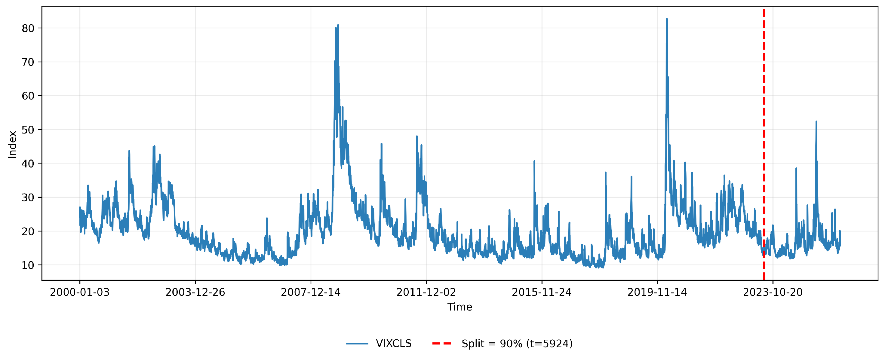
Figure 1 shows in-sample (training set) and out-of-sample (test set) division to train and test our model in the VIXCLS dataset. We split the full dataset in a training set of 90% (5923 observations) and a test set of 10% (650 observations), as shown in Figure 1.

Realized variance measures constructed from high-frequency data have become a standard observable proxy for latent volatility and are known to display several stylized empirical features, including strong persistence, heavy right tails, and nonlinear dynamics with volatility clustering and asymmetric adjustments following large shocks (Andersen et al., 2003; Barndorff-Nielsen & Shephard, 2002). These properties often challenge linear autoregressive specifications and motivate forecasting approaches capable of accommodating flexible marginal distributions and nonlinear temporal dependence.

The empirical autoregressive copula proposed in this paper is designed to address these features directly. By transforming the observed series through its empirical distribution function, the model separates marginal behavior from temporal dependence and estimates the lag–lead dependence structure nonparametrically on the copula scale. This approach allows the transition density of the process to adapt flexibly to asymmetric and state-dependent dynamics commonly observed in realized volatility data, without imposing restrictive parametric assumptions on the dependence structure.

To assess the empirical relevance of this flexibility, we compare the proposed empirical autoregressive copula against a range of benchmark models commonly used in volatility forecasting, including parametric copula specifications, linear autoregressive models, and state-space or conditional-heteroskedasticity models.

Emp–MAP is the empirical copula model with a one-step mode forecast on the copula scale: given $u_{t-1}$, we select ${\widehat{u}}_t^{\mathrm{MAP}}\left(u_{t-1}\right)=arg{max}_{v\in (0,1)}{\widehat{f}}_{U_{t-1},U_t}(u_{t-1},v)$ on a uniform grid and map it back to the data scale by ${\widehat{x}}_t={\widehat{F}}^{-1}\left({\widehat{u}}_t^{\mathrm{MAP}}\right)$. Emp–MEAN is the empirical copula model with a conditional-mean forecast on the original scale, computed via LOTUS as ${\widehat{x}}_t^{\mathrm{mean}}\left(u_{t-1}\right)=\mathbb{E}[X_t\mid U_{t-1}=u_{t-1}]\approx {\int }_0^1{\widehat{F}}^{-1}\left(v\right)\widehat{f}(v\mid u_{t-1})dv$, implemented numerically on the same grid used for the KDE-based conditional density.

As parametric dependence benchmarks on the uniform scale, Gaus–cop and t–cop denote autoregressive copula models in which the lag–lead dependence of $(U_{t-1},U_t)$ is modeled with a Gaussian copula and a Student’s-t copula, respectively, with parameters estimated from the training sample and used to generate multi-step forecasts via the implied conditional distribution.

AR(1) and ARMA(1, 1) are linear models fitted to the original series, while ARMA-BIC is selected by minimizing the Bayesian information criterion over a grid of ARMA$(p,q)$ specifications with $p,q\in \{0,\dots ,6\}$ on the training sample.

We additionally include three state-space/conditional-heteroskedasticity benchmarks that are commonly used to capture time variation in persistence and uncertainty. First, TVP–AR(1) denotes a time-varying-parameter autoregression,

$$X_t={\alpha }_t+{\varphi }_t{X}_{t-1}+{\epsilon }_t,\left(\begin{array}{c}{\alpha }_t\\ {\varphi }_t\end{array}\right)=\left(\begin{array}{c}{\alpha }_{t-1}\\ {\varphi }_{t-1}\end{array}\right)+{\eta }_t,$$

estimated on the training sample in a linear Gaussian state-space form and filtered via the Kalman filter; multi-step forecasts are obtained recursively using the filtered state at each forecast origin. Second, Local level is the standard random-walk level model,

$$X_t={\mu }_t+{\epsilon }_t,{\mu }_t={\mu }_{t-1}+{\xi }_t,$$

which serves as a parsimonious baseline for slow-moving dynamics and is likewise estimated and forecast using Kalman filtering. Finally, ARMA–GARCH refers to an ARMA$(1,1)$ model for the conditional mean coupled with a GARCH$(1,1)$ conditional variance specification, estimated by quasi-maximum likelihood on the training sample and used to generate rolling multi-step forecasts under the fitted conditional mean dynamics.

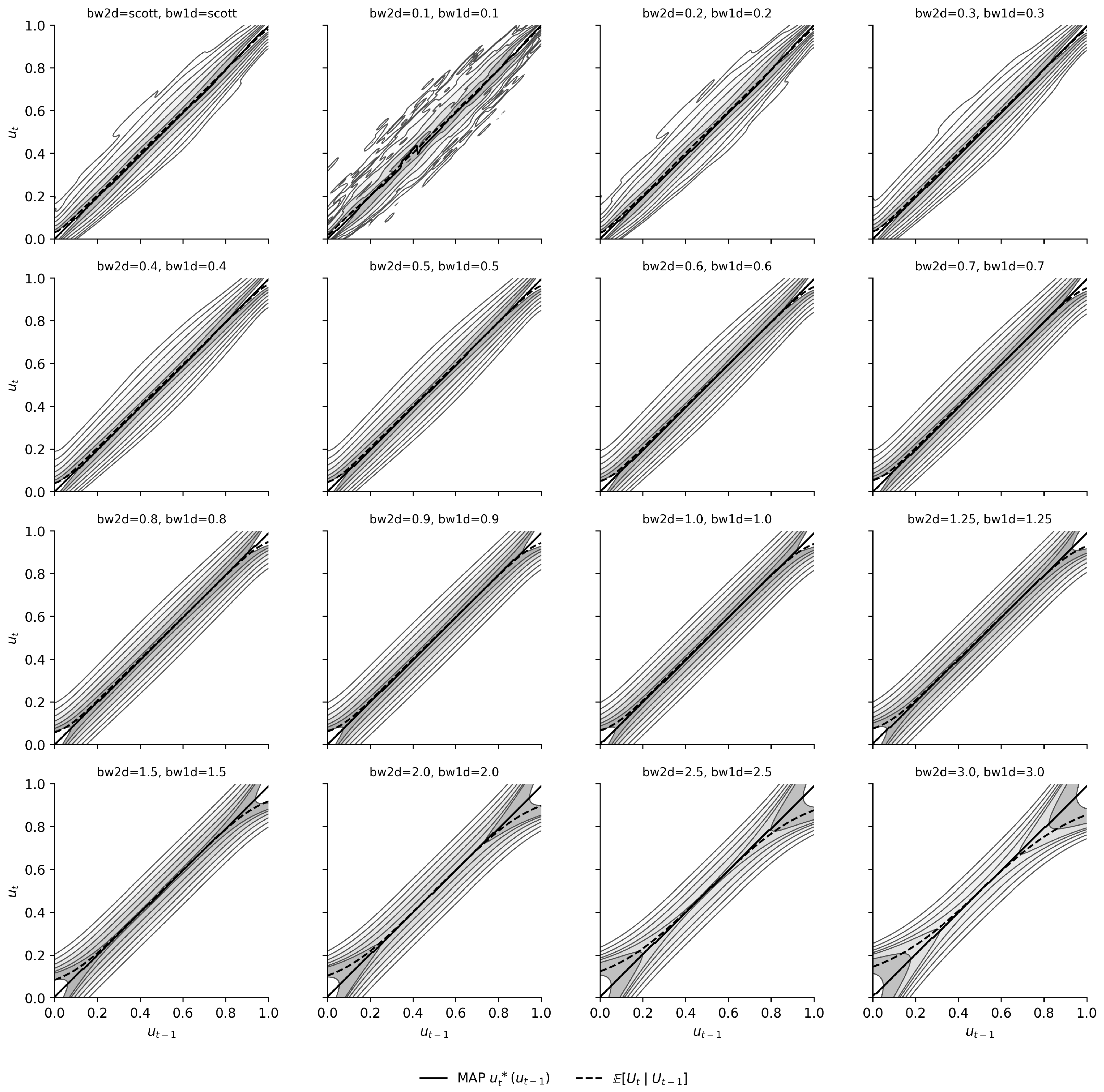
Figure 2 shows the estimated conditional copula density $c(u_t\mid u_{t-1})$ fitted to the VIX and evaluated on a uniform grid for different bandwidth choices, together with the one-step MAP curve ${\widehat{u}}_t^{\mathrm{MAP}}\left(u_{t-1}\right)=arg{max}_{v\in (0,1)}c(v\mid u_{t-1})$ and the conditional-mean curve $\mathbb{E}[U_t\mid U_{t-1}=u_{t-1}]$. The MAP curve maps each $u_{t-1}$ to the most likely $u_t$ under the estimated conditional density, and it forms the basis for our one-step forecasts on the copula scale (subsequently mapped back to the data scale via ${\widehat{F}}^{-1}$).

It is apparent that the choice of bandwidth materially affects the smoothness and shape of the estimated nonparametric copula surface, and consequently the implied conditional dependence captured by $c(u_t\mid u_{t-1})$.

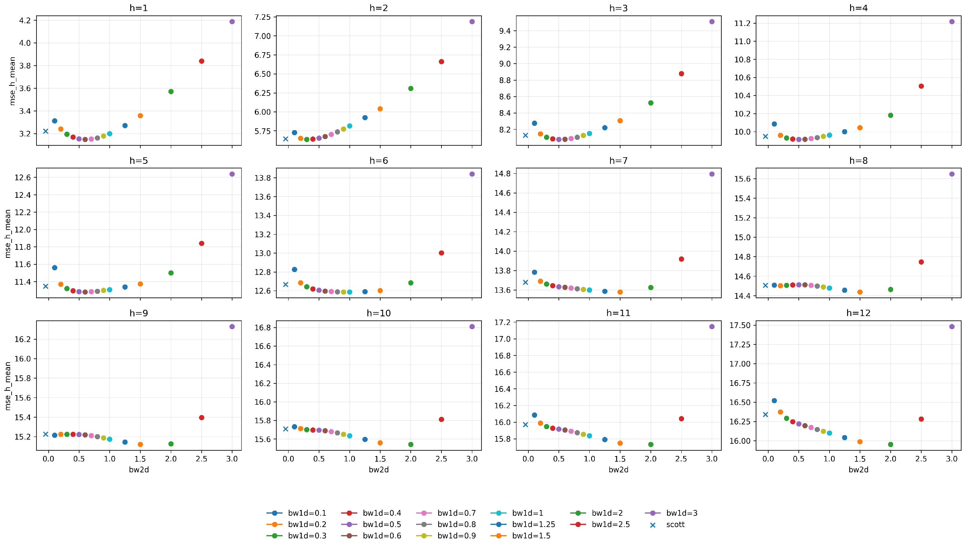
For this reason, it becomes necessary to assess, through a sensitivity analysis, how the empirical copula’s predictive performance varies across different bandwidth specifications. To this end, we compare candidate bandwidth pairs using the copula model’s mean squared forecast error (MSE) as the performance metric. The results reveal differences across bandwidth choices, indicating that a careful calibration of the smoothing parameters is warranted. This sensitivity is summarized in

Table 1. Bandwidth grid: aggregated in-sample error (mean MSE across horizons). We impose $b{w}_{2d}=b{w}_{1d}=bw$. Best result in bold.

$\mathbf{bw}$	MSE (MEAN)	MSE (MAP)
scott	11.865593	14.998321
0.10	11.969321	14.523762
0.20	11.878931	15.504579
0.30	11.847038	13.999539
0.40	11.831408	13.398811
0.50	11.824366	13.334170
0.60	11.820722	13.190815
0.70	11.818706	13.090890
0.80	11.818024	12.928483
0.90	11.818712	12.727256
1.00	11.820703	12.550114
1.25	11.830329	12.225057
1.50	11.846739	12.078321
2.00	11.934583	11.926187
2.50	12.243648	11.854875
3.00	13.066220	11.829976

.

For the VIXCLS series, we find that a bandwidth of $0.8$ provides the best overall performance, while for RVXCLS and VXDCLS the preferred values are $2.5$ and $1.0$, respectively. This provides further evidence that the bandwidth parameter should be calibrated in a series-specific manner, reflecting differences in the underlying dependence structure across markets.

It is also noteworthy that the optimal bandwidth may vary across forecast horizons, as shown in Figure 3, suggesting that a horizon-specific calibration could, in principle, yield additional gains. Nevertheless, to keep the benchmarking exercise parsimonious and comparable across models, we restrict attention to the bandwidth choice that minimizes the average training MSE across the 12 forecast horizons.

Table 2. MSE out-of-sample (horizons 1–12). The best (lowest) MSE in each horizon is in bold, second best marked with an asterisk.

Series	Model h	AR(1)	ARIMA–BIC	ARMA(1, 1)	ARMA–GARCH	Emp–MAP	Emp–MEAN	Gaus–Cop	Local Level	TVP–AR(1)	t–Cop
RVXCLS	1	2.346	2.352	2.353	2.312 *	2.249	2.760	2.323	2.382	2.407	2.331
	2	4.268	4.295	4.301	4.183	4.094	4.470	4.115 *	4.401	5.103	4.149
	3	6.153	6.194	6.194	5.969	5.867	6.031	5.795	6.410	8.329	5.857 *
	4	7.823	7.874	7.876	7.518	7.394	7.230 *	7.214	8.243	11.184	7.315
	5	9.185	9.294	9.298	8.791	8.590	8.177	8.326 *	9.843	13.561	8.457
	6	10.557	10.706	10.707	10.034	9.835	9.117	9.460 *	11.461	16.128	9.615
	7	11.752	11.914	11.917	11.107	10.870	9.847	10.395 *	12.897	18.664	10.580
	8	12.553	12.774	12.782	11.886	11.649	10.450	11.042 *	13.986	20.366	11.233
	9	13.334	13.610	13.621	12.629	12.404	10.976	11.634 *	15.067	22.167	11.837
	10	14.044	14.365	14.378	13.322	13.124	11.460	12.170 *	16.076	23.586	12.384
	11	14.594	14.951	14.968	13.905	13.655	11.825	12.577 *	16.913	24.646	12.796
	12	14.956	15.366	15.388	14.354	14.071	12.075	12.857 *	17.569	25.542	13.077
VIXCLS	1	3.358	3.338	3.350	3.249	3.103	3.149 *	3.279	3.393	3.613	3.301
	2	5.908	5.893	5.976	5.634	5.749	5.676 *	5.711	6.135	9.691	5.776
	3	8.724	8.595	8.748	8.122 *	8.403	8.080	8.227	9.086	22.307	8.380
	4	10.820	10.643	10.860	9.931 *	10.428	9.917	9.998	11.423	38.036	10.216
	5	12.543	12.358	12.622	11.392 *	12.110	11.281	11.403	13.436	63.053	11.697
	6	14.014	13.830	14.134	12.635	13.749	12.597	12.613 *	15.225	106.128	12.950
	7	15.264	15.078	15.402	13.695	15.105	13.627 *	13.552	16.785	176.570	13.915
	8	16.079	15.986	16.295	14.473 *	16.264	14.512	14.251	17.959	293.262	14.585
	9	16.989	16.919	17.231	15.258	17.327	15.219 *	14.916	19.200	494.118	15.263
	10	17.606	17.600	17.889	15.839	18.119	15.690 *	15.344	20.141	833.364	15.691
	11	18.096	18.152	18.435	16.323	18.664	15.906 *	15.639	20.966	1410.976	16.003
	12	18.632	18.714	19.002	16.837	19.269	16.196 *	15.983	21.825	2397.511	16.360
VXDCLS	1	4.721	4.365 *	4.359	4.563	4.611	4.535	4.748	4.391	7.971	4.757
	2	6.155	5.763	5.846	5.854	5.932	5.782 *	6.029	5.947	7.446	6.109
	3	7.606	7.105 *	7.247	7.107	7.247	7.044	7.293	7.442	12.060	7.442
	4	8.390	7.857	8.111	7.761 *	7.943	7.713	7.952	8.404	13.077	8.134
	5	9.539	8.945	9.246	8.708 *	8.951	8.598	8.909	9.667	15.959	9.160
	6	10.251	9.733	10.059	9.301 *	9.607	9.250	9.439	10.608	18.109	9.713
	7	11.505	10.855	11.243	10.293	10.871	10.379 *	10.473	11.964	20.712	10.786
	8	12.006	11.364	11.741	10.709	11.405	10.898	10.884 *	12.582	21.299	11.167
	9	12.352	11.748	12.099	10.978	11.663	11.152	11.125 *	13.047	22.569	11.392
	10	12.635	12.111	12.448	11.220	11.920	11.353	11.318 *	13.508	22.865	11.556
	11	13.358	12.756	13.132	11.764	12.497	11.804 *	11.907	14.356	24.542	12.163
	12	13.664	13.068	13.445	11.996 *	12.697	11.938	12.115	14.777	25.421	12.341

reports the out-of-sample mean squared error (MSE) for the proposed empirical autoregressive copula and a set of competing benchmarks across forecast horizons $h=1,\dots ,12$ for three volatility-index series (RVXCLS, VIXCLS, and VXDCLS). For each horizon and dataset, the smallest MSE is highlighted in bold, while the second-best result is marked with an asterisk, facilitating a direct comparison of forecasting accuracy across models and lead times.

Overall, the results indicate that the proposed nonparametric copula approach is either the best performer or very close to the best across most horizons and datasets, which highlights its ability to recover nonlinear lag–lead dependence structures in volatility dynamics. In particular, Emp–MEAN frequently attains the lowest MSE (notably for RVXCLS and many horizons of VIXCLS), while Emp–MAP often remains among the top performers at short horizons, suggesting that both the conditional-mean and mode-based copula forecasts provide competitive accuracy depending on the lead time and the series. Parametric copula competitors (Gaus–Cop and t–Cop) and classical linear benchmarks (AR/ARMA/ARMA–GARCH) can be competitive in specific cases, but they typically do not dominate systematically across horizons. By contrast, TVP–AR(1) tends to yield the largest errors, especially at longer horizons. A plausible explanation is that volatility indices exhibit pronounced spikes and regime-like behavior; in such episodes, Kalman updates can drive the filtered autoregressive coefficient ${\varphi }_t$ close to a unit root, or even temporarily above one, which effectively induces locally nonstationary forecast dynamics. This can amplify multi-step forecast errors even when the underlying series is globally stationary, helping to explain the comparatively weak performance of the TVP benchmark in this setting.

Importantly, the performance gap between copula-based and linear models tends to widen with h, suggesting that modeling dependence on the uniform scale captures nonlinear serial features that are not well represented by standard linear dynamics.

Table 3. MAE out-of-sample (horizons 1–12). The best (lowest) MSE in each horizon is in bold, second best marked with an asterisk.

Series	Model h	AR(1)	ARIMA–BIC	ARMA(1, 1)	ARMA–GARCH	Emp–MAP	Emp–MEAN	Gaus–Cop	Local Level	TVP–AR(1)	t–Cop
RVXCLS	1	0.944	0.944	0.944	0.933 *	0.932	1.156	0.950	0.949	1.022	0.948
	2	1.312	1.319	1.321	1.289	1.282	1.386	1.293 *	1.333	1.337	1.296
	3	1.599	1.610	1.610	1.560	1.545	1.613	1.540	1.641	1.697	1.547 *
	4	1.815	1.826	1.828	1.777	1.762 *	1.772	1.735	1.873	1.943	1.745
	5	1.995	2.015	2.017	1.948	1.931	1.895 *	1.893	2.078	2.159	1.908
	6	2.173	2.188	2.189	2.095	2.059	2.021 *	2.011	2.267	2.358	2.035
	7	2.304	2.318	2.318	2.221	2.181	2.104	2.124 *	2.413	2.523	2.150
	8	2.371	2.392	2.393	2.284	2.261	2.153	2.182 *	2.501	2.610	2.205
	9	2.449	2.478	2.480	2.362	2.346	2.210	2.250 *	2.605	2.710	2.275
	10	2.538	2.569	2.571	2.450	2.430	2.269	2.320 *	2.713	2.833	2.350
	11	2.627	2.664	2.667	2.527	2.492	2.321	2.380 *	2.822	2.931	2.413
	12	2.690	2.730	2.733	2.586	2.530	2.348	2.404 *	2.915	3.041	2.441
VIXCLS	1	0.987	0.988	0.988	0.957	0.963 *	0.994	0.989	0.987	1.116	0.987
	2	1.372	1.374	1.378	1.316	1.342	1.340 *	1.359	1.382	1.461	1.359
	3	1.677	1.677	1.685	1.574	1.616	1.607 *	1.628	1.706	1.903	1.637
	4	1.898	1.900	1.898	1.787	1.850	1.812 *	1.832	1.927	2.226	1.840
	5	2.098	2.087	2.095	1.955	2.033	1.980 *	2.004	2.139	2.545	2.016
	6	2.276	2.254	2.272	2.081	2.214	2.128 *	2.149	2.330	2.841	2.167
	7	2.426	2.384	2.409	2.189	2.361	2.249 *	2.278	2.467	3.148	2.296
	8	2.509	2.472	2.495	2.257	2.453	2.319 *	2.334	2.570	3.424	2.352
	9	2.605	2.561	2.586	2.336	2.556	2.388 *	2.405	2.658	3.729	2.423
	10	2.672	2.624	2.650	2.395	2.616	2.433 *	2.462	2.719	4.085	2.475
	11	2.754	2.695	2.726	2.454	2.674	2.472 *	2.522	2.788	4.511	2.539
	12	2.839	2.772	2.807	2.504	2.721	2.517 *	2.582	2.863	5.068	2.596
VXDCLS	1	1.125	1.104	1.102	1.099 *	1.109	1.130	1.134	1.097	1.564	1.129
	2	1.395	1.362	1.374	1.342	1.359 *	1.378	1.395	1.372	1.370	1.392
	3	1.624	1.577	1.596	1.522	1.549 *	1.587	1.606	1.597	1.803	1.606
	4	1.734	1.690	1.706	1.630	1.660 *	1.694	1.715	1.711	1.827	1.711
	5	1.874	1.828	1.844	1.762	1.794 *	1.817	1.844	1.870	2.041	1.837
	6	1.983	1.926	1.956	1.815	1.863 *	1.908	1.928	1.975	2.116	1.926
	7	2.137	2.057	2.093	1.938	2.007 *	2.045	2.078	2.120	2.313	2.072
	8	2.221	2.136	2.176	1.987	2.077 *	2.124	2.147	2.210	2.366	2.143
	9	2.260	2.171	2.209	2.019	2.105 *	2.157	2.185	2.240	2.409	2.169
	10	2.317	2.229	2.267	2.055	2.140 *	2.200	2.239	2.299	2.470	2.219
	11	2.423	2.315	2.361	2.117	2.224 *	2.275	2.343	2.397	2.569	2.320
	12	2.498	2.377	2.427	2.139	2.243 *	2.320	2.409	2.438	2.606	2.380

reports the out-of-sample mean absolute error (MAE) for the proposed empirical autoregressive copula and the full set of competing benchmarks across horizons $h=1,\dots ,12$ for RVXCLS, VIXCLS, and VXDCLS. As in the MSE table, the best (lowest) MAE in each horizon is highlighted in bold, while the second-best result is indicated with an asterisk, enabling a horizon-by-horizon assessment of forecasting accuracy under an absolute-loss criterion.

The MAE results broadly corroborate the conclusions obtained under squared loss. The empirical copula forecasts remain dominant or very close to the best performer in the majority of horizons and datasets, reinforcing that the proposed nonparametric dependence model learns forecasting-relevant patterns that are often only partially captured by standard time-series specifications. At the same time, the ARMA–GARCH benchmark becomes more competitive under MAE and attains the best performance in several horizons (particularly for VIXCLS and VXDCLS). Nevertheless, even in horizons where ARMA–GARCH is best, the empirical copula variants typically remain second-best or very close to the minimum MAE, highlighting the robustness of the copula-based approach relative to more parametric and structurally heavier alternatives.

To assess whether differences in forecast accuracy are statistically meaningful, we apply the Diebold–Mariano (DM) test to compare each competing model against the Emp–MEAN baseline at each horizon h. We compute the DM statistic using the Harvey–Leybourne–Newbold small-sample correction (Harvey et al., 1997), we estimate the long-run variance of the loss differential with a Bartlett HAC estimator. Reported p-values correspond to a one-sided alternative and should be interpreted descriptively given the multiple horizons and model comparisons.

Let $e_{t,h}^{\mathrm{base}}$ and $e_{t,h}^{\mathrm{model}}$ denote the h-step-ahead forecast errors of the baseline and a competing model, respectively, and let $L\left(·\right)$ be the loss function (squared-error loss in our implementation). We define the loss differential as

$$d_{t,h}=L\left(e_{t,h}^{\mathrm{base}}\right)-L\left(e_{t,h}^{\mathrm{model}}\right),$$

so that $d_{t,h}<0$ indicates that the baseline (Emp–MEAN) attains lower loss than the competing model at time t. The DM test evaluates the null hypothesis $\mathbb{E}\left[d_{t,h}\right]=0$ using a HAC variance estimator. Under this convention, a negative DM statistic favors the baseline (Emp–MEAN), whereas a positive statistic favors the competing model. Under the one-sided alternative used here, small p-values provide evidence that Emp–MEAN significantly outperforms the competitor (i.e., $\mathbb{E}\left[d_{t,h}\right]<0$).

Table A1. Diebold–Mariano (one-sided) for VIXCLS. Baseline: Emp–MEAN. Loss: squared error. Cells show DM statistic with p-value in parentheses.

h	AR(1)	ARIMA–BIC	ARMA(1, 1)	ARMA–GARCH	Emp–MAP	Gaus–Cop	Local Level	TVP–AR(1)	t–Cop
1	−0.505 (0.307)	−0.546 (0.293)	−0.520 (0.302)	−3.914 (0.000)	0.349 (0.636)	−0.360 (0.359)	−4.234 (0.000)	−4.112 (0.000)	−0.399 (0.345)
2	−0.636 (0.263)	−0.902 (0.184)	−1.029 (0.152)	−2.975 (0.002)	−0.468 (0.320)	−0.138 (0.445)	−3.469 (0.000)	−2.763 (0.003)	−0.335 (0.369)
3	−1.737 (0.041)	−1.801 (0.036)	−1.902 (0.029)	−3.234 (0.001)	−2.306 (0.011)	−0.962 (0.168)	−3.589 (0.000)	−2.021 (0.022)	−1.372 (0.085)
4	−1.443 (0.075)	−1.557 (0.060)	−1.499 (0.067)	−2.754 (0.003)	−2.479 (0.007)	−0.377 (0.353)	−3.274 (0.001)	−1.633 (0.051)	−0.918 (0.180)
5	−1.497 (0.067)	−1.675 (0.047)	−1.578 (0.058)	−2.247 (0.012)	−3.348 (0.000)	−0.470 (0.319)	−2.958 (0.002)	−1.423 (0.078)	−0.968 (0.167)
6	−1.662 (0.048)	−1.824 (0.034)	−1.751 (0.040)	−1.908 (0.028)	−3.575 (0.000)	−0.070 (0.472)	−2.942 (0.002)	−1.268 (0.103)	−0.894 (0.186)
7	−1.707 (0.044)	−1.799 (0.036)	−1.817 (0.035)	−1.677 (0.047)	−3.658 (0.000)	0.362 (0.641)	−2.795 (0.003)	−1.180 (0.119)	−0.771 (0.220)
8	−1.801 (0.036)	−1.729 (0.042)	−1.882 (0.030)	−1.329 (0.092)	−3.544 (0.000)	1.610 (0.946)	−2.466 (0.007)	−1.113 (0.133)	−0.288 (0.387)
9	−1.761 (0.039)	−1.600 (0.055)	−1.789 (0.037)	−1.069 (0.143)	−3.545 (0.000)	1.573 (0.942)	−2.126 (0.017)	−1.073 (0.142)	−0.154 (0.439)
10	−1.702 (0.045)	−1.506 (0.066)	−1.687 (0.046)	−1.028 (0.152)	−3.509 (0.000)	1.564 (0.941)	−1.945 (0.026)	−1.045 (0.148)	−0.004 (0.498)
11	−1.644 (0.050)	−1.467 (0.071)	−1.619 (0.053)	−1.159 (0.123)	−3.453 (0.000)	0.995 (0.840)	−1.916 (0.028)	−1.026 (0.153)	−0.255 (0.400)
12	−1.605 (0.055)	−1.435 (0.076)	−1.576 (0.058)	−1.316 (0.094)	−3.371 (0.000)	0.674 (0.750)	−1.887 (0.030)	−1.013 (0.156)	−0.370 (0.356)

in the Appendix A provides one-sided Diebold–Mariano tests comparing each competitor to the Emp–MEAN baseline under squared-error loss for the VIXCLS serie. Across essentially all horizons, the estimated DM statistics are negative for the competing models, and the p-values are frequently below conventional significance levels, especially from intermediate to long horizons. In particular, the linear benchmarks—AR(1), ARMA(1, 1), and ARIMA–BIC—exhibit negative DM statistics with borderline-to-small p-values from roughly $h=3$ onward (e.g., $h=3$ to $h=12$), indicating that their forecast accuracy is statistically inferior to Emp–MEAN at these horizons.

The evidence is even stronger against the state-space and conditional-heteroskedasticity benchmarks: both the Local level and TVP–AR(1) models display large negative DM statistics with very small p-values throughout all horizons, implying clear rejection of the hypothesis that they are at least as accurate as Emp–MEAN. Likewise, ARMA–GARCH shows strongly negative DM statistics with p-values essentially zero at short horizons and remaining small for several horizons, supporting the conclusion that the empirical copula mean forecast delivers superior predictive accuracy for VIXCLS under squared loss. Finally, the parametric copula alternatives (Gaus–Cop and t–Cop) also yield negative statistics across horizons, with limited or no evidence that they outperform the baseline; overall, the DM tests support Emp–MEAN as the dominant specification for VIXCLS in this benchmark set.

For RVXCLS (

Table A2. Diebold–Mariano (one-sided) for RVXCLS. Baseline: Emp–MEAN. Loss: squared error. Cells show DM statistic with p-value in parentheses.

h	AR(1)	ARIMA–BIC	ARMA(1, 1)	ARMA–GARCH	Emp–MAP	Gaus–Cop	Local Level	TVP–AR(1)	t–Cop
1	1.651 (0.950)	1.673 (0.953)	1.694 (0.955)	−2.997 (0.001)	2.848 (0.998)	1.820 (0.965)	−3.327 (0.000)	−3.463 (0.000)	1.745 (0.959)
2	0.655 (0.744)	0.614 (0.730)	0.603 (0.727)	−2.756 (0.003)	1.445 (0.925)	1.232 (0.891)	−3.460 (0.000)	−2.653 (0.004)	1.099 (0.864)
3	−0.281 (0.390)	−0.391 (0.348)	−0.394 (0.347)	−2.781 (0.003)	0.437 (0.669)	0.576 (0.718)	−3.593 (0.000)	−2.051 (0.020)	0.417 (0.661)
4	−1.066 (0.143)	−1.209 (0.114)	−1.226 (0.110)	−3.251 (0.001)	−0.364 (0.358)	0.032 (0.513)	−3.878 (0.000)	−1.931 (0.027)	−0.175 (0.431)
5	−1.811 (0.035)	−2.050 (0.020)	−2.076 (0.019)	−3.207 (0.001)	−0.919 (0.179)	−0.350 (0.363)	−3.860 (0.000)	−1.873 (0.031)	−0.640 (0.261)
6	−2.305 (0.011)	−2.476 (0.007)	−2.489 (0.007)	−3.272 (0.001)	−1.523 (0.064)	−0.785 (0.216)	−3.465 (0.000)	−1.745 (0.041)	−1.104 (0.135)
7	−2.399 (0.008)	−2.520 (0.006)	−2.532 (0.006)	−3.048 (0.001)	−2.020 (0.022)	−1.172 (0.121)	−3.368 (0.000)	−1.671 (0.048)	−1.473 (0.071)
8	−2.332 (0.010)	−2.478 (0.007)	−2.493 (0.006)	−3.146 (0.001)	−2.172 (0.015)	−1.180 (0.119)	−3.349 (0.000)	−1.655 (0.049)	−1.449 (0.074)
9	−2.380 (0.009)	−2.540 (0.006)	−2.554 (0.005)	−3.286 (0.001)	−2.466 (0.007)	−1.351 (0.089)	−3.335 (0.000)	−1.673 (0.047)	−1.622 (0.053)
10	−2.506 (0.006)	−2.646 (0.004)	−2.653 (0.004)	−3.224 (0.001)	−2.819 (0.002)	−1.625 (0.052)	−3.162 (0.001)	−1.719 (0.043)	−1.937 (0.027)
11	−2.575 (0.005)	−2.659 (0.004)	−2.660 (0.004)	−2.977 (0.002)	−3.056 (0.001)	−2.055 (0.020)	−2.940 (0.002)	−1.738 (0.041)	−2.452 (0.007)
12	−2.498 (0.006)	−2.567 (0.005)	−2.562 (0.005)	−2.864 (0.002)	−3.221 (0.001)	−2.387 (0.009)	−2.802 (0.003)	−1.761 (0.039)	−2.821 (0.002)

in the Appendix A), the one-sided DM results similarly favor the Emp–MEAN baseline. From mid to long horizons, most competitors exhibit negative DM statistics accompanied by small p-values, implying that their performance is significantly worse than the baseline. This pattern is particularly pronounced for the linear ARMA-family benchmarks (AR(1), ARMA(1, 1), and ARIMA–BIC), where the p-values fall below $10\%$ from approximately $h=5$ onward, consistently rejecting the null hypothesis that these models are at least as accurate as Emp–MEAN.

The strongest rejections occur for Local level and TVP–AR(1), which present large negative DM statistics with p-values effectively zero across the entire horizon range, indicating that these state-space benchmarks underperform the empirical copula baseline decisively for RVXCLS. The ARMA–GARCH benchmark also shows negative DM statistics with very small p-values at all horizons, reinforcing that incorporating conditional heteroskedasticity in this parametric way does not close the gap to the nonparametric copula baseline in this dataset. Regarding the alternative copula competitors, Gaus–Cop and t–Cop become significantly worse than Emp–MEAN at longer horizons (with p-values below $10\%$ for higher h), whereas Emp–MAP does not show evidence of improving upon Emp–MEAN (negative DM statistics with small p-values in the long horizon range). Taken together, the DM tests confirm that Emp–MEAN is statistically superior to most competitors for RVXCLS, especially for medium and long prediction horizons.

Table A3. Diebold–Mariano (one-sided) for VXDCLS. Baseline: Emp–MEAN. Loss: squared error. Cells show DM statistic with p-value in parentheses.

h	AR(1)	ARIMA–BIC	ARMA(1, 1)	ARMA–GARCH	Emp–MAP	Gaus–Cop	Local Level	TVP–AR(1)	t–Cop
1	−0.854 (0.197)	0.750 (0.773)	0.690 (0.755)	−1.717 (0.043)	−0.601 (0.274)	−0.889 (0.187)	−1.696 (0.045)	−3.767 (0.000)	−0.924 (0.178)
2	−1.218 (0.112)	0.061 (0.524)	−0.323 (0.374)	−1.945 (0.026)	−0.899 (0.184)	−1.104 (0.135)	−2.139 (0.016)	−2.053 (0.020)	−1.216 (0.112)
3	−1.616 (0.053)	−0.263 (0.396)	−0.762 (0.223)	−1.460 (0.072)	−1.014 (0.155)	−1.137 (0.128)	−2.012 (0.022)	−2.172 (0.015)	−1.428 (0.077)
4	−1.553 (0.060)	−0.431 (0.333)	−1.006 (0.157)	−1.948 (0.026)	−0.907 (0.182)	−0.968 (0.167)	−2.397 (0.008)	−1.928 (0.027)	−1.270 (0.102)
5	−1.652 (0.049)	−0.823 (0.205)	−1.217 (0.112)	−1.092 (0.138)	−1.298 (0.097)	−1.122 (0.131)	−2.065 (0.020)	−1.809 (0.035)	−1.368 (0.086)
6	−1.695 (0.045)	−1.093 (0.137)	−1.458 (0.073)	−1.720 (0.043)	−0.937 (0.174)	−0.755 (0.225)	−2.743 (0.003)	−1.855 (0.032)	−1.202 (0.115)
7	−1.758 (0.040)	−0.909 (0.182)	−1.420 (0.078)	−0.686 (0.247)	−1.100 (0.136)	−0.372 (0.355)	−2.330 (0.010)	−1.789 (0.037)	−1.068 (0.143)
8	−1.860 (0.032)	−0.819 (0.207)	−1.397 (0.081)	−0.201 (0.420)	−0.830 (0.203)	0.172 (0.568)	−1.901 (0.029)	−1.658 (0.049)	−0.879 (0.190)
9	−1.753 (0.040)	−0.845 (0.199)	−1.305 (0.096)	−0.125 (0.450)	−0.687 (0.246)	0.248 (0.598)	−1.765 (0.039)	−1.683 (0.046)	−0.715 (0.237)
10	−1.710 (0.044)	−0.927 (0.177)	−1.319 (0.094)	−0.567 (0.285)	−0.588 (0.278)	0.294 (0.616)	−1.893 (0.029)	−1.626 (0.052)	−0.558 (0.289)
11	−1.749 (0.040)	−0.968 (0.167)	−1.322 (0.093)	−0.249 (0.402)	−0.634 (0.263)	−0.326 (0.372)	−1.595 (0.056)	−1.553 (0.060)	−0.892 (0.186)
12	−1.712 (0.044)	−1.012 (0.156)	−1.323 (0.093)	−0.434 (0.332)	−0.644 (0.260)	−0.578 (0.282)	−1.684 (0.046)	−1.517 (0.065)	−0.925 (0.178)

in Appendix A reports one-sided DM tests for VXDCLS series. The results again mostly support Emp–MEAN as the preferred benchmark: the majority of competitors produce negative DM statistics, and several horizons exhibit p-values below $10\%$, implying statistically significant underperformance relative to the empirical copula mean forecast. In particular, the AR(1) benchmark shows negative DM statistics with p-values below $10\%$ for a broad set of horizons (e.g., $h=3$–$h=12$), while the state-space models (Local level and TVP–AR(1)) present consistently negative statistics with small p-values throughout, indicating clear inferiority of these alternatives under squared-error loss.

For the remaining competitors, the evidence is more mixed in the sense that some p-values are not small at certain horizons; however, the sign of the DM statistic is generally negative, so the lack of significance should be interpreted as “insufficient evidence to conclude a difference” rather than evidence in favor of the competitor. Notably, neither ARIMA–BIC nor the parametric copula alternatives (Gaus–Cop and t–Cop) display systematic positive DM statistics with small p-values; hence, there is no horizon range in which they can be said to outperform Emp–MEAN in a statistically supported way. Overall, the one-sided DM tests for VXDCLS corroborate the forecast-error tables: the empirical nonparametric copula baseline is typically either strictly better (often significantly so) or statistically indistinguishable from the best competitor, with the clearest advantages emerging at intermediate and longer horizons.

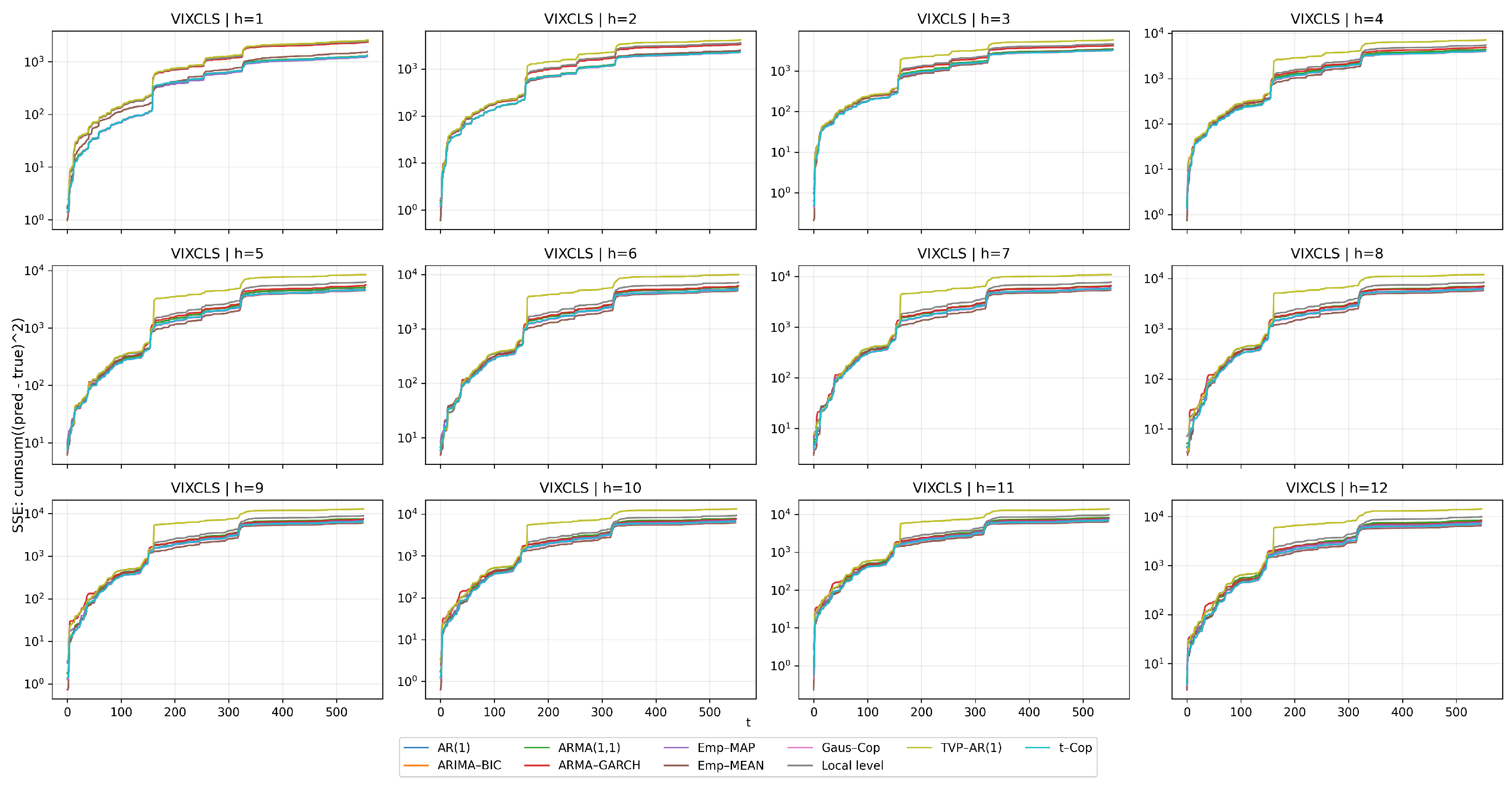
The cumulative squared error curves (Figure 4) indicate that the separation across competing models becomes markedly more pronounced during episodes associated with large volatility shocks. In these periods, the accumulated loss rises sharply and the gaps between methods widen, suggesting that misspecification is amplified when the data exhibit abrupt, nonlinear dynamics. Notably, the nonlinear specifications track these large volatility shocks more effectively, yielding systematically lower cumulative errors around the largest jumps. This pattern is clearly visible in Figure 4, where nonlinear models maintain a tighter trajectory through high-volatility intervals relative to their linear counterparts.

4. Conclusions

We proposed a fully nonparametric empirical autoregressive copula framework for univariate time series. The approach combines a shape-preserving empirical marginal distribution (implemented via monotone interpolation) with a boundary-reflected kernel density estimator for the lag–lead dependence on the uniform scale. This construction yields forecasts that respect the empirical support and preserve the marginal shape through back-transformation, while allowing for flexible nonlinear serial dependence without imposing parametric copula restrictions.

Conceptually, the framework reframes autoregressive modeling as the estimation of a conditional transport mechanism induced by the empirical copula. Forecasts arise as functionals of the estimated conditional density—in particular, conditional modes (Emp–MAP) and conditional means (Emp–MEAN)—rather than from explicit parametric recursion equations. This perspective emphasizes the geometry of transitions over parameter dynamics and provides a probabilistically coherent way to capture nonlinear persistence and asymmetric adjustments that are typical in volatility-like series.

Empirically, we evaluated the method on three daily CBOE volatility indices (VIXCLS, VXDCLS, and RVXCLS) and compared it against nonlinear copula competitors (Gaussian and Student’s-t autoregressive copulas) as well as standard linear benchmarks (AR(1), ARMA(1, 1), and ARMA–BIC). In addition, we incorporated three widely used state-space/conditional-heteroskedasticity models (Local level, TVP–AR(1), and ARMA(1, 1)–GARCH(1, 1)) to benchmark against time-varying persistence and conditional variance specifications. Across datasets and horizons, the empirical copula forecasts are consistently among the best performers under both MSE and MAE criteria, often achieving the lowest error and, when not first, remaining close to the best competitor. This pattern highlights that modeling the full transition density on the copula scale can recover dependence structures that are otherwise only partially captured by more rigid parametric dynamics.

A key practical implication is that bandwidth selection materially affects the estimated copula surface and therefore forecast performance. Our sensitivity analysis over a grid of bandwidth values shows nontrivial dispersion in in-sample error, and the bandwidth that minimizes average training MSE differs across series, reinforcing the need for series-specific calibration. While horizon-specific bandwidth choices could in principle deliver additional gains, we adopt a parsimonious strategy and select the bandwidth that minimizes the average training MSE across the 12 forecast horizons to ensure comparability across models.

Finally, one-sided Diebold–Mariano tests provide formal evidence supporting the empirical copula baseline. Under squared-error loss and using Emp–MEAN as the reference, the tests frequently reject the hypothesis that competing models are at least as accurate as the baseline, particularly for the state-space benchmarks (Local level and TVP–AR(1)) and for linear ARMA-family models at medium and longer horizons. These results are aligned with the out-of-sample error tables: although some competitors may appear competitive at isolated horizons, the empirical copula forecast is difficult to match systematically across horizons and across volatility indices. In particular, the weaker performance of TVP–AR(1) is consistent with the sensitivity of Kalman updates to volatility spikes, which can push the filtered persistence parameter close to (or above) the unit-root boundary and generate large multi-step forecast errors.

While the proposed framework provides a flexible approach for modeling nonlinear autoregressive dependence, several limitations should be noted. First, the empirical specification adopts a first-order Markov structure, which may not fully capture the longer memory dynamics often observed in financial volatility processes. Second, although the nonparametric copula approach allows for considerable flexibility in modeling dependence, its extension to higher-order autoregressive structures may be affected by the curse of dimensionality. Third, as with most kernel-based methods, the performance of the estimator depends on the selection of bandwidth parameters, which may influence finite-sample results. Finally, the present study focuses primarily on the empirical performance of the proposed methodology, and a complete asymptotic theory for the estimator is left for future research. Investigating these theoretical properties and exploring extensions to more complex dynamic structures represent promising directions for further methodological development.

An important extension of the proposed framework would consist in moving from the univariate setting considered in this paper to a multivariate dynamic specification. In particular, the model could be extended to jointly describe the dynamics of volatility indices and asset returns within a multivariate copula-based autoregressive structure. Such an extension would allow the analysis of nonlinear dependence and tail co-movements between financial markets and volatility measures such as the VIX. In this context, the transition dynamics of the multivariate process could be represented through copula functions linking current observations to their lagged values, thereby enabling the estimation of state-dependent dependence structures and tail dependence patterns. This framework would provide a natural setting for studying contagion effects and volatility spillovers across markets. From a methodological perspective, scalable multivariate constructions such as vine copulas (Aas, 2016; Brechmann & Czado, 2015; Czado et al., 2019) or factor copula models (Krupskii & Joe, 2013) could be combined with the autoregressive copula structure developed in this paper in order to maintain flexibility while controlling dimensionality.

Overall, the proposed framework provides a transparent and probabilistically interpretable nonparametric baseline for forecasting observed volatility proxies in settings where nonlinear dependence and boundary effects are central. By combining nonparametric marginal estimation with a copula-based representation of the transition density, the methodology offers a flexible approach for modeling dynamic dependence structures while remaining robust to marginal misspecification. Future research may explore principled bandwidth selection methods, higher-order autoregressive extensions on the copula scale, and multivariate generalizations capable of capturing cross-market dependence and tail co-movements. More broadly, the proposed approach opens the door to nonparametric conditional density modeling in time-series environments where probabilistic coherence, interpretability, and flexibility are key modeling objectives.