Citywide Air Quality Forecasting over Sparse Sensor Networks: Cross-Location Generalization and Deep Learning Reliability Under Missing Data

Abstract

Smart city environmental monitoring depends on sparse air quality sensor networks and analytics services that remain reliable under node additions, outages, and missing streams. We propose an operational deep learning framework for citywide cross-location forecasting from a limited set of sensors, delivering low-latency, real-time concentration heatmaps at unsensed locations by combining temporal prediction with spatial regression. We formulate single-stage spatiotemporal forecasting and benchmark nine recurrent, convolutional, and multilayer architectures against classical baselines. The framework forecasts ${\mathrm{O}}_3$, ${\mathrm{NO}}_2$, ${\mathrm{PM}}_{2.5}$, and ${\mathrm{PM}}_{10}$ over horizons from 1 h to 10 days. Using open monitoring data from Madrid (Spain) and Cali (Colombia), we evaluate generalization by holding out stations, reflecting deployment to new sensor nodes and sparse coverage regimes. We further compare missing data handling strategies and show that common imputation can substantially degrade accuracy, increasing RMSE by up to 74% in some settings. Beyond prediction, the framework provides a basis for guiding sensor network densification; confidence estimates can highlight locations where additional sensors may be most beneficial. These results provide actionable guidance for deploying AI-enabled sensing services with robust performance under realistic sensor reliability constraints while supporting real-time citywide mapping.

1. Introduction

The growing trend of urbanization is evident, with approximately 58% of the global population residing in cities as of 2024, according to the United Nations Population Division [1]. Urbanization and industrialization pose challenges such as traffic congestion, healthcare demands, and air quality issues. To tackle these problems and enhance urban living standards, continuous environmental monitoring—from traffic flow to air quality—is essential. Smart cities increasingly leverage the Internet of Things (IoT) to deploy sensor networks comprising monitoring stations that gather data for analysis and support informed decision-making. Many cities have installed air quality sensors that measure various pollutants, and these data are often made publicly accessible, enabling officials, automated platforms, and individuals to take action. This is especially important for vulnerable populations, such as the elderly, children, and those with respiratory conditions, who may experience adverse health effects even at pollution levels considered safe for the general population. In this context, modeling frameworks capable of processing sensor data and delivering timely, actionable insights play a crucial role in urban environmental management.

Forecasting pollutant levels not only provides governments and citizens with more time to take reactive measures, but it also enables proactive strategies to mitigate adverse outcomes. Many major cities have been forced to implement emergency interventions due to pollution episodes, such as traffic restrictions in New Delhi in November 2024 [2,3]. Consequently, research has increasingly focused on urban air quality prediction, particularly in densely populated regions such as India [4], China [5,6], and Tehran [7,8]. Deep learning (DL), a subset of machine learning (ML) based on complex neural networks (NNs), has proven especially effective for modeling frameworks that must manage high-volume, multivariate environmental data, due to its ability to extract high-level patterns from extensive datasets [9,10].

It should be noted that predicting air quality is subject to several limitations. Air pollution is inherently complex, influenced by multiple factors, including natural and anthropogenic sources. Most predictive models rely on extensive historical datasets, as shown in Table 1, where many referenced studies require several years of data. The use of large datasets also increases computational complexity. Additionally, air quality datasets, which span long periods and depend on distributed sensor networks, often contain many missing values. There are additional pain points specific to sparse sensor air quality monitoring. First, the limited number of stations produces incomplete spatial coverage, making it difficult to estimate pollutant levels at unmonitored locations. Second, monitoring streams often contain outages and missing values, which can severely reduce the amount of usable training data or distort the temporal structure when naïve imputation is applied. Third, pollutant dynamics are governed by nonlinear interactions between local emissions, meteorology, and spatial transport, which are difficult to capture with simple interpolation or shallow predictive models. Finally, from a deployment perspective, a useful smart-city system must generalize to locations not seen during training while still supporting low-latency prediction over the whole city but leveraging the shared characteristics of nearby sensors remains challenging due to potential nonlinear spatial correlations among air quality monitoring sites [10].

1.1. Related Work

Numerous papers have addressed air pollutant forecasting, many using deep learning or Bayesian spatiotemporal models. Table 1 contains a summary of the referenced air quality publications. Drewil and Al-Bahadili [4] used genetic algorithms to select the best parameters for an long short-term memory (LSTM) model and predicted four pollutants one day in advance using data between 2017 and 2020. They only tested an LSTM architecture, and found that their proposed NN gave better prediction results than when the parameters were manually fine-tuned. Similarly, the study by Tao et al. [11] predicted ${\mathrm{PM}}_{2.5}$ levels using a convolutional-based bidirectional gated recurrent unit (GRU) and Bhatta et al. [12] evaluated different machine learning approaches. However, these works only consider the time dimension.

Table 1. Related works on air quality prediction. For each study, we analyze whether fine-grained cross-location spatial prediction is used to estimate the level of pollutants in places where there are no sensors, or at least whether spatial prediction is used to estimate the pollution at one or multiple locations with a sensor. When air quality forecasting is used, the time lag is expressed in hours, days, or months. We compare which studies require only fixed stations, the pollutants predicted, whether they use deep learning (DL) models, and the length of the dataset used.

Authors	Cross-Location Spatial Prediction	Forecasting	Only Uses Fixed Stations	Predicted Pollutants	DL Models	Data Length
Bougoudis et al. [13]	Multiple stations	1 h	Yes	CO, NO, ${\mathrm{O}}_3$, ${\mathrm{NO}}_2$, ${\mathrm{SO}}_2$	No	∼11 years
Apte et al. [14]	Fine-grained	No	No	BC, NO, ${\mathrm{NO}}_2$	No	1 year
Hu et al. [15]	Fine-grained	1 d	No	${\mathrm{PM}}_{2.5}$	No	1 year
Nicolis et al. [16]	Fine-grained	1 d	Yes	${\mathrm{PM}}_{2.5}$	No	2.5 months
Tao et al. [11]	No	2 h	Yes	${\mathrm{PM}}_{2.5}$	Yes	5 years
Kalajdjieski et al. [17]	No	No	Yes	${\mathrm{PM}}_{2.5}$	Yes	2 years
Bekkar et al. [5]	One station	1 d, 7 d	Yes	${\mathrm{PM}}_{2.5}$	Yes	4 years
Fioravanti et al. [18]	Fine-grained	No	Yes	${\mathrm{PM}}_{10}$	No	1 year
Shahriar et al. [19]	Multiple stations	1 d	Yes	${\mathrm{PM}}_{2.5}$	Yes	6.5 years
Wan et al. [6]	Multiple stations	1 h, 2 h, 3 h	Yes	${\mathrm{PM}}_{2.5}$	No	2 years
Drewil and Al-Bahadili [4]	No	1 d	Yes	${\mathrm{PM}}_{2.5}$, ${\mathrm{PM}}_{10}$, CO, NOX	Yes	∼3 years
Kristiani et al. [20]	No	8 h	Yes	${\mathrm{PM}}_{2.5}$	Yes	∼2 years
Saez and Barceló [21]	Fine-grained	No	Yes	${\mathrm{O}}_3$, ${\mathrm{NO}}_2$, ${\mathrm{PM}}_{2.5}$, ${\mathrm{PM}}_{10}$	No	∼10 years
Baniasadi et al. [7]	Fine-grained	1 d	Yes	${\mathrm{PM}}_{2.5}$	Yes	10 years
Kumar and Pande [22]	No	No	Yes	AQI	No	6 years
Samad et al. [23]	Multiple stations	No	Yes	${\mathrm{NO}}_2$, ${\mathrm{PM}}_{2.5}$, ${\mathrm{PM}}_{10}$	No	4.25 years
Rabie et al. [8]	No	1 y	Yes	AQI	Yes	5 years
Rahman et al. [24]	No	No	Yes	AQI, AQC	No	23,463 instances
Wu et al. [25]	Fine-grained	4 d, 7 d, 10 d, 14 d	No	${\mathrm{PM}}_{2.5}$	Yes	∼6 years
Yang et al. [26]	Fine-grained	1 h	No	${\mathrm{PM}}_{2.5}$	No	Up to 9 months
Zareba et al. [27]	Multiple stations	1 d	Yes	${\mathrm{PM}}_{2.5}$	Yes	10 years
Illescas-Martinez et al. [28]	Fine-grained	No	Yes	${\mathrm{O}}_3$, ${\mathrm{NO}}_2$, ${\mathrm{PM}}_{2.5}$, ${\mathrm{PM}}_{10}$	Yes	9 years
Xia et al. [29]	No	1 h–2 d	Yes	${\mathrm{NO}}_2$, ${\mathrm{PM}}_{2.5}$, ${\mathrm{PM}}_{10}$	Yes	Up to 3 years
Zhang et al. [30]	Fine-grained	4 h–1 d	No	${\mathrm{NO}}_2$	Yes	1 year
Bhatta et al. [12]	No	1 d	Yes	${\mathrm{PM}}_{2.5}$	No	5 years
Panja et al. [31]	Multiple stations	30–90 d	Yes	${\mathrm{NO}}_2$, ${\mathrm{PM}}_{2.5}$, ${\mathrm{PM}}_{10}$	Yes	4 years
This work	Fine-grained	1 h, 2 h, 1 d, 4 d, 7 d, 10 d	Yes	${\mathrm{O}}_3$, ${\mathrm{NO}}_2$, ${\mathrm{PM}}_{2.5}$, ${\mathrm{PM}}_{10}$	Yes	Up to 6 months

Table 1. Related works on air quality prediction. For each study, we analyze whether fine-grained cross-location spatial prediction is used to estimate the level of pollutants in places where there are no sensors, or at least whether spatial prediction is used to estimate the pollution at one or multiple locations with a sensor. When air quality forecasting is used, the time lag is expressed in hours, days, or months. We compare which studies require only fixed stations, the pollutants predicted, whether they use deep learning (DL) models, and the length of the dataset used.

Authors	Cross-Location Spatial Prediction	Forecasting	Only Uses Fixed Stations	Predicted Pollutants	DL Models	Data Length
Bougoudis et al. [13]	Multiple stations	1 h	Yes	CO, NO, ${\mathrm{O}}_3$, ${\mathrm{NO}}_2$, ${\mathrm{SO}}_2$	No	∼11 years
Apte et al. [14]	Fine-grained	No	No	BC, NO, ${\mathrm{NO}}_2$	No	1 year
Hu et al. [15]	Fine-grained	1 d	No	${\mathrm{PM}}_{2.5}$	No	1 year
Nicolis et al. [16]	Fine-grained	1 d	Yes	${\mathrm{PM}}_{2.5}$	No	2.5 months
Tao et al. [11]	No	2 h	Yes	${\mathrm{PM}}_{2.5}$	Yes	5 years
Kalajdjieski et al. [17]	No	No	Yes	${\mathrm{PM}}_{2.5}$	Yes	2 years
Bekkar et al. [5]	One station	1 d, 7 d	Yes	${\mathrm{PM}}_{2.5}$	Yes	4 years
Fioravanti et al. [18]	Fine-grained	No	Yes	${\mathrm{PM}}_{10}$	No	1 year
Shahriar et al. [19]	Multiple stations	1 d	Yes	${\mathrm{PM}}_{2.5}$	Yes	6.5 years
Wan et al. [6]	Multiple stations	1 h, 2 h, 3 h	Yes	${\mathrm{PM}}_{2.5}$	No	2 years
Drewil and Al-Bahadili [4]	No	1 d	Yes	${\mathrm{PM}}_{2.5}$, ${\mathrm{PM}}_{10}$, CO, NOX	Yes	∼3 years
Kristiani et al. [20]	No	8 h	Yes	${\mathrm{PM}}_{2.5}$	Yes	∼2 years
Saez and Barceló [21]	Fine-grained	No	Yes	${\mathrm{O}}_3$, ${\mathrm{NO}}_2$, ${\mathrm{PM}}_{2.5}$, ${\mathrm{PM}}_{10}$	No	∼10 years
Baniasadi et al. [7]	Fine-grained	1 d	Yes	${\mathrm{PM}}_{2.5}$	Yes	10 years
Kumar and Pande [22]	No	No	Yes	AQI	No	6 years
Samad et al. [23]	Multiple stations	No	Yes	${\mathrm{NO}}_2$, ${\mathrm{PM}}_{2.5}$, ${\mathrm{PM}}_{10}$	No	4.25 years
Rabie et al. [8]	No	1 y	Yes	AQI	Yes	5 years
Rahman et al. [24]	No	No	Yes	AQI, AQC	No	23,463 instances
Wu et al. [25]	Fine-grained	4 d, 7 d, 10 d, 14 d	No	${\mathrm{PM}}_{2.5}$	Yes	∼6 years
Yang et al. [26]	Fine-grained	1 h	No	${\mathrm{PM}}_{2.5}$	No	Up to 9 months
Zareba et al. [27]	Multiple stations	1 d	Yes	${\mathrm{PM}}_{2.5}$	Yes	10 years
Illescas-Martinez et al. [28]	Fine-grained	No	Yes	${\mathrm{O}}_3$, ${\mathrm{NO}}_2$, ${\mathrm{PM}}_{2.5}$, ${\mathrm{PM}}_{10}$	Yes	9 years
Xia et al. [29]	No	1 h–2 d	Yes	${\mathrm{NO}}_2$, ${\mathrm{PM}}_{2.5}$, ${\mathrm{PM}}_{10}$	Yes	Up to 3 years
Zhang et al. [30]	Fine-grained	4 h–1 d	No	${\mathrm{NO}}_2$	Yes	1 year
Bhatta et al. [12]	No	1 d	Yes	${\mathrm{PM}}_{2.5}$	No	5 years
Panja et al. [31]	Multiple stations	30–90 d	Yes	${\mathrm{NO}}_2$, ${\mathrm{PM}}_{2.5}$, ${\mathrm{PM}}_{10}$	Yes	4 years
This work	Fine-grained	1 h, 2 h, 1 d, 4 d, 7 d, 10 d	Yes	${\mathrm{O}}_3$, ${\mathrm{NO}}_2$, ${\mathrm{PM}}_{2.5}$, ${\mathrm{PM}}_{10}$	Yes	Up to 6 months

However, urban air pollution exhibits significant spatial variability, often within distances of less than 1 km. This strong spatial variability leads to difficulties complain with the European Air Quality Directive, that requires that “a sampling point must be sited in such a way that the air sampled is representative of air quality for a street segment no less than 100 m in length at traffic-oriented sites” [32]. This is due to the uneven distribution of emission sources, dilution, and environmental factors. Conventional fixed-site monitoring lacks the resolution to detect such localized pollution variations [14]; however, covering entire urban areas with high-density sensing networks would be economically and logistically prohibitive. Studies have explored alternative methods for detailed air quality assessment, such as equipping Google Street View mapping vehicles with air quality measurement tools [14]. To add a spatial dimension to NNs, Baniasadi et al. [7] fine-tuned an LSTM architecture and optimized its parameters using a binary chimp optimization algorithm. However, they interpolated pollution levels throughout Tehran using the Kriging method, a geostatistical linear interpolation method for estimating values at unmeasured locations based on known data points.

Bekkar et al. [5] were able to predict ${\mathrm{PM}}_{2.5}$ using different deep learning algorithms; they added an additional spatial dimension to the study by incorporating data from different stations to predict ${\mathrm{PM}}_{2.5}$ in a single station. This offered great results in forecasting particulate matter up to a week in advance, but it was employed to predict air quality at a single point rather than throughout the city. Wan et al. [6] developed a spatio-temporal model to predict ${\mathrm{PM}}_{2.5}$ concentrations in Beijing, taking into account air pollutants, meteorological variables, and geographical conditions. The model used data from the previous hour from multiple sensors to estimate current ${\mathrm{PM}}_{2.5}$ levels. Rabie et al. [8] divided the Tehran megacity in three regions, and they used different DL models to predict the Air Quality Index (AQI) up to one year in advance.

In the work by Zareba et al. [27], global forecasting models (GFMs) were used to predict ${\mathrm{PM}}_{2.5}$ levels in the city of Krakow. A GFM is a model that facilitates the concurrent construction of a unified predictive model for multiple, geographically dispersed time series. This means it forecasts all the time series simultaneously. Its objective is to capture the fundamental patterns governing the series, thereby minimizing the potential noise from each series. This methodological framework enabled the authors to effectively forecast air quality in regions with monitoring stations. The work by Shahriar et al. [19] explored the potential of ARIMA-ANN, ARIMA-SVM, Principal Component Regression, Decision Trees, and CatBoost for forecasting ${\mathrm{PM}}_{2.5}$ concentrations in Bangladesh. Similarly, Kristiani et al. [20] DL methods for ${\mathrm{PM}}_{2.5}$ forecasting in Taiwan. Panja et al. [31] trained spatio-temporal graph convolutional networks to predict long-term air pollution data in 37 monitoring stations across Delhi with a focus on extreme pollutant levels. However, these models can only make predictions in locations where a sensor is placed, they cannot be used to make spatially continuous predictions.

Other works focused on offering more spatially detailed levels of air quality but disregarded the temporal dimension. This allowed pollution levels in regions without stations to be spatially predicted, with the spatial domain ranging from cities to countries. Saez and Barceló [21] used a hierarchical Bayesian spatiotemporal model to predict short- and long-term exposure through different Basic Health Areas in Catalonia, Spain.

Alternatively, the study by Fioravanti et al. [18] employed a Bayesian hierarchical spatio-temporal model to predict daily air pollution concentrations. Namely, they proposed 12 statistical models (one per month) to predict ${\mathrm{PM}}_{10}$ across a $1 \mathrm{k}\mathrm{m} \times 1 \mathrm{k}\mathrm{m}$ grid over Italy. A similar analysis had previously been applied to Santiago de Chile (Nicolis et al. [16]) for ${\mathrm{PM}}_{2.5}$ concentrations, where the authors predicted hourly concentrations one day in advance.

Each of these studies took a distinct approach to air quality prediction. The work by Samad et al. [23] sought to foresee different pollutants using several monitoring stations throughout the city to predict pollution in a few locations where other stations were present. They concluded that the pollutants from other monitoring stations as an input feature played a significant role in the estimation and, more interestingly, they observed that the same ML models were able to estimate pollutant concentrations at other locations as well. Hence, the technique could be transferred to other locations where pollutant prediction is required. However, it must be mentioned that each place has its own particularities, whether geographic, urban, or demographic. For example, in the work by Wan et al. [6], the altitude of each point was used as a factor in predicting ${\mathrm{PM}}_{2.5}$ in the mountainous city of Beijing, but this information is likely to be of no interest in a city located on a plateau, such as Madrid. Furthermore, the number of monitoring stations varies depending on the size of the city and the resources invested. Therefore, in this study, we have analyzed different cities with different sizes and number of stations and compared the results.

A limited number of studies have combined forecasting and spatial predictions to determine the level of pollution that will cover an entire area using a limited number of fixed monitoring stations. These include the previously mentioned study by Baniasadi et al. [7], which used an LSTM model for forecasting and interpolation for the spatial dimension, and the one by Nicolis et al. [16], which used a Bayesian hierarchical spatio-temporal model to predict daily concentrations of air pollution one day in advance. Other approaches include the spatio-temporal air pollution DL model proposed by Zhang et al. [30] for easter China, which uses spaceborne remote sensing data combined with supplementary weather datasets, and the random forest (RF) model by Hu et al. [15], which combines data from monitoring stations that have been randomly divided into training and validation sets, as well as satellite-derived aerosol optical depth. Xia et al. [29] developed a synchronous graph transformer network to forecast air pollution in a multistep approach, and their results assumed constant pollution across a region.

Recent research by Yang et al. [26] used a Nested Air Quality Prediction Modeling System (a multi-scale air quality modeling system for reproducing atmospheric pollutant transport and evolution) to conduct several sensitivity experiments. This allowed the analysis and comparison of different measures to prevent and reduce air pollution. However, this required meticulous modeling of the area and pollution transfer. A data-driven approach can be implemented more quickly, and DL can learn to model complex transport and evolution dynamics. Finally, the study by Wu et al. [25] aimed to forecast ${\mathrm{PM}}_{2.5}$ levels in the forested Heilongjiang Province. The authors focused on forest fires, using these fires as auxiliary inputs for their LSTM model. They favorably tested their model against other architectures and empirically chose the time lag. The analysis revealed that the lowest root mean squared error (RMSE) was achieved with a seven-day forecast rather than a four-day forecast, as might have been expected.

In contrast, the present work formulates spatiotemporal prediction as a single supervised learning problem in which temporal histories from multiple stations and the spatial relation to the target location are processed jointly by one model. This distinction is important because it avoids decoupling temporal forecasting errors from a second interpolation stage and allows the model to learn temporal and cross-location dependencies simultaneously. This makes the approach easily implementable and transferable to other cities, as it relies on routinely available measurements without requiring additional infrastructure. While each model is tailored to a specific city with a fixed number of monitoring stations arranged in a canonical order, the trained weights from one city can also be used to initialize models for other cities, facilitating transfer learning and reducing training effort.

1.2. Contributions

In this work, we propose a DL modeling framework for fine-grained cross-location air quality forecasting that predicts future concentrations of ${\mathrm{O}}_3$, ${\mathrm{NO}}_2$, ${\mathrm{PM}}_{2.5}$, and ${\mathrm{PM}}_{10}$ at arbitrary target locations, including locations without sensors, by learning spatial–temporal dependencies from sparse fixed-station networks. By “cross-location”, we refer to the model’s ability to exploit measurements from multiple monitoring sites to forecast pollutant levels at other (possibly unmonitored) locations. By “fine-grained”, we mean that predictions can be generated on a dense spatial grid, enabling continuous citywide coverage and forecasted air quality heatmaps.

Therefore, this work addresses a practical gap in city-scale air quality prediction under sparse sensing conditions: how to forecast pollutant concentrations at future times and at locations without sensors using only the historical measurements from a limited set of fixed stations. The methodological novelty of this paper is not the introduction of a new neural architecture; instead, it lies in a unified problem formulation and deployment-oriented pipeline that integrates temporal forecasting and cross-location spatial regression in a single model. This approach enables the neural network to concurrently model the temporal evolution and cross-location spatial transfer, facilitating the learning of complex dynamics that could be compromised by the division of the pipeline into temporal and spatial steps. We train and validate on a subset of stations and evaluate on entirely unseen stations, so the test set reflects genuinely unmonitored locations.

Existing studies on air quality prediction span a broad spectrum of methods for temporal forecasting and spatial estimation. While combining spatial and temporal dimensions provides a more complete understanding, the complex, nonlinear dynamics of air pollution often limit the effectiveness of linear models. Our approach addresses this by leveraging deep learning models capable of capturing complex spatial-temporal relationships using only data from fixed sensors. Building on the spatial regression setup of Illescas-Martinez et al. [28], our system extends it to temporal forecasting, enabling future predictions at unobserved locations using only fixed-station data. Additionally, we obtained our results using shorter datasets than those used in many of the works analyzed in Table 1, which lowers the data-collection burden and facilitates deployment.

We evaluate the approach in two cities—Madrid, Spain and Cali, Colombia—which differ in sensor density, geography, and sample size. To support reproducibility, the dataset is publicly released in Zenodo [33]. We further benchmark recurrent and convolutional architectures (convolutional neural network (CNN), GRU, LSTM, Multipath-CNN-LSTM (MCNNLSTM), GRU×2, LSTM×2, LSTMGRU, bidirectional long short-term memory (BiLSTM)) against classical baselines (naïve forecast, RF, linear regression (LR)) to identify robust configurations across pollutants and forecast horizons (1 h, 2 h, 1 day, 4 days, 7 days, and 10 days).

In this context, the main contributions of this paper are summarized below:

• We formulate and implement a single-stage DL regression model that jointly learns temporal dependencies from multi-station histories and spatial transfer to a target location via distance-conditioned inputs, enabling forecasting at unmonitored locations without requiring mobile sensing or dense deployments.
• We provide an end-to-end pipeline (from sparse fixed-station data preprocessing and sample construction to citywide forecasted heatmap generation) and evaluate generalization under a strict hold-out-location setting, where test sensors are never seen during training/validation, reflecting realistic deployment to unmonitored areas.
• We demonstrate the practical potential of the proposed system to support real-world monitoring by enabling the generation of fine-grained citywide pollution heatmaps and by reporting low inference times that make near real-time heatmap updates feasible.
• We perform a comprehensive comparison of deep NN architectures and classical baselines across cities, pollutants, and horizons, and we quantify the impact of missing-data strategies, showing that common imputation can substantially degrade forecasting accuracy and that data quality may outweigh data quantity.
• We complement performance results with model interpretability analyses using permutation importance and shapley additive explanations (SHAP), clarifying which input variables and past timesteps most influence predictions across pollutants and cities.

The rest of the paper is organized as follows. Section 2 discusses the different deep learning models analyzed in this work, and Section 3 describes the detailed methodology for the proposed approach. Results are provided in Section 4, and Section 5 concludes the paper.

2. Deep Learning Models

In this section, we briefly discuss the different DL models that have been examined in this study. We adopted the model architectures and hyperparameters reported by Illescas-Martinez et al. [28], where the hyperparameters had been tuned using a Random Search strategy. That work investigated cross-location air pollutant prediction, facilitating the inference of city-wide air quality heatmaps. The present study builds upon that foundation by integrating temporal forecasting with spatial prediction, and focuses on comparing architectures, cities, and missing-data strategies under a consistent configuration.

DL becomes saturated when inappropriate activation functions are selected [9,34]. To avoid this problem, the activation layer has been set as ReLU when applicable, except for the output layer, where it has been set as sigmoid, thereby restricting the output to the known range of values. Weights were initialized using the Glorot Uniform initializer, which has been shown to improve convergence in deep networks (Glorot and Bengio [34]). Mean squared error (MSE) was selected as the loss metric, as it is standard for regression tasks, and RMSprop was used as the optimizer due to its proven performance in air quality forecasting scenarios [11]. The output layer is a dense layer with a single unit, appropriate for predicting a single continuous value. A summary of the deep learning architectures is provided in

Table 2. Summary of deep learning architectures.

Model	Architecture Description
CNN	1D Conv (64 filters, kernel size 3) → MaxPool (size 2)
	→ Dense (32) → Dense (16) → Output
GRU	GRU (64 units) → Dense (32) → Output
LSTM	LSTM (64 units) → Dense (32) → Output
MCNNLSTM	CNN path: 1D Conv (64, 3) → MaxPool (2) → Dense (32)
	+ LSTM path: LSTM (64) → Dropout (drop rate 0.2) → GAP1D
	→ Concatenate → Output
MCNNLSTMv2	CNN path: 1D Conv (64, 3) → 1D Conv (32, 3) → Dense (16)
	+ LSTM path: LSTM (64) → Dropout (0.1) → Dense (32) → Dense (16)
	→ Concatenate → Dense (8) → Output
GRU×2	GRU (64) → GRU (32) → Dropout (0.2) → Output
LSTM×2	LSTM (64) → LSTM (32) → Dropout (0.2) → Output
LSTMGRU	LSTM (64) → GRU (32) → Dense (32) → Dropout (0.2) → Output
BiLSTM	Bidirectional LSTM (64) → Dropout (0.2) → Output

at the end of this section.

All DL experiments used the same training configuration: RMSprop optimizer, batch size 64, early stopping patience 100, and TensorFlow default optimizer parameters (learning rate 0.001, rho 0.9, momentum 0.0, epsilon $1\times {10}^{-7}$), so that the comparison across architectures, pollutants, and time horizons isolates the effect of model design rather than changes in architecture or optimization settings. The maximum number of epochs was set high enough that early stopping always acted as the termination criterion. Loss-versus-epoch plots for the trained models are provided in [35] to illustrate training performance.

2.1. CNN

A convolutional layer is a layer within an artificial neural network that applies convolutions to the input. Convolution involves sliding a filter or kernel across the input, which is typically a two-dimensional or three-dimensional matrix, and performing a scalar product between the filter and the region of the input it covers. In the model in this paper, the convolutional layers have been constructed using one-dimensional kernels that move through the sequence (unlike images where 2D convolutions are used). These kernels act as filters that learn during training.

The CNN model in this paper uses a 1D convolutional layer with 64 filters with a kernel size of 3, followed by a Max Pool of size 2, a dense layer with 32 nodes, a dense layer with 16 nodes, and the output layer.

2.2. GRU

While the convolutional layer focuses on extracting local features and spatial patterns, GRU is a recurrent layer used in recurrent neural networks (RNNs) that adds a temporal dimension to the analysis. A GRU layer is a gating mechanism consisting of two gates: an update gate (z) and a reset gate (r). The update gate decides which information gets transferred to the next hidden state, while the reset gate determines the information to be discarded from the previous hidden state. The GRU layer also has a candidate unit ($\stackrel{\sim }{\mathrm{h}}$), which computes the candidate hidden state based on the current input and the previous hidden state. The final hidden state (h) is achieved by combining the previous hidden state and the candidate hidden state according to the update gate.

The GRU model in this paper uses a GRU layer with 64 units, followed by a dense layer with 32 nodes, and the output layer.

2.3. LSTM

An LSTM layer is a recurrent neural network capable of learning and retaining long-term dependencies within sequential data, such as text, audio, or time series. In addition to the hidden state in traditional RNNs, an LSTM has three gates: an input gate that determines whether to let the new input in, a forget gate that deletes unimportant information, and an output gate that decides what information to output. These three gates are analogical gates based on the sigmoid function, which works in the range between 0 and 1. These gates are structures composed of linear layers and activation functions that regulate the flow of information between the cells of the LSTM layer.

The LSTM model in this paper uses an LSTM layer with 64 units, followed by a dense layer with 32 nodes, and the output layer.

2.4. MCNNLSTM

Classical CNN architecture is usually considered the best choice when the input networks are 2D or 3D tensors like images or videos. Since LSTM architectures are better adapted for 1D data, there are multiple approaches to combining CNN and LSTM that attempt to incorporate the positive aspects of both NNs. In this work, we opt for processing the input of both layers simultaneously and then concatenating the results, which are finally processed by a dense layer.

The Multipath-CNN-LSTM model in this paper uses a 1D convolutional layer with 64 filters with a kernel size of 3, followed by a Max Pool of size 2, and a dense layer with 32 nodes (similar to the proposed CNN). In parallel, we use an LSTM layer with 64 units, followed by a dropout layer with a drop rate of 0.2 and a global average pooling 1D layer. Both outputs are concatenated and connected to the output layer. This model is referred to as MCNNLSTM.

Alternatively, the MCNNLSTMv2 model in this paper uses a 1D convolutional layer with 64 filters with a kernel size of 3, followed by a 1D convolutional layer with 32 filters with a kernel size of 3 and a dense layer with 16 nodes. In parallel, we use an LSTM layer with 64 units, followed by a dropout layer with a drop rate of 0.1, a dense layer with 32 nodes, and a dense layer with 16 nodes. Both outputs are concatenated and connected to a dense layer with 8 nodes, followed by the output layer.

2.5. GRU×2

Using two consecutive GRU layers enhances the model’s ability to capture complex temporal dependencies in sequential data. The first GRU layer processes the input sequence and extracts temporal patterns, while the second layer refines these patterns by modeling higher-level representations. This hierarchical structure allows the model to learn short-term and long-term dependencies more effectively, allowing for improved predictive accuracy.

The GRU×2 model in this paper uses a GRU layer with 64 units, followed by a GRU layer with 32 units, a dropout layer with a drop rate of 0.2, and the output layer.

2.6. LSTM×2

Similar to the GRU×2 model, the LSTM×2 model in this paper uses an LSTM layer with 64 units, followed by an LSTM layer with 32 units, a dropout layer with a drop rate of 0.2, and the output layer.

2.7. LSTMGRU

Like the previous models, combining two consecutive recurrent layers may improve predictive accuracy. The LSTMGRU model in this paper uses an LSTM layer with 64 units, followed by a GRU layer with 32 units, a dense layer with 32 units, a dropout layer with a drop rate of 0.2, and the output layer.

2.8. BiLSTM

Standard RNNs and LSTMs often ignore future information during temporal processing; however, BiLSTMs are capable of leveraging future information. In essence, a BiLSTM is a sequence processing model consisting of two LSTMs, one taking the input in a forward direction and the other in a backward direction. BiLSTMs effectively increase the amount of information available to the network, improving the context available to the algorithm. Moreover, both LSTMs are connected to an input and output layer, enabling the output layer to obtain past information from each point of the input sequence and obtain future information from each point through this structure.

The BiLSTM model in this paper uses a bidirectional LSTM layer with 64 units, followed by a dropout layer with a drop rate of 0.2, and the output layer.

3. Materials and Methods

Our dataset consists of 213,297 records from two cities—Madrid, Spain and Cali, Colombia—collected via the AQI India API [36], which provides transparent access to air quality measurements independently of the original data source. As a result, the retrieved records may originate from heterogeneous sources, including official air quality monitoring stations and other sensing devices such as user-deployed or IoT sensors. Since the API does not systematically provide metadata describing the sensing technology or analyzer used at each station, the present work does not distinguish between data sources and treats all measurements uniformly within the proposed framework. Nevertheless, most of the data used in this study come from the official monitoring stations deployed by the town halls of Madrid and Cali for their respective cities.

Table 3. Data origin for the different cities.

City	Input Sensors	Label Sensors	Test Sensors	Start Date	End Date
Cali	7	2	9	13/06/2024	17/12/2024
Madrid	10	3	2	25/11/2024	17/12/2024

indicates the number of sensors per city and the time interval when the values were recorded. The data from most stations are used to create a training dataset, employed for training and validation. A summary of the data statistics is presented in

Table 4. Summary statistics of air pollutants and meteorological data in air pollution monitoring sites after outlier removal. The data are stored with a precision of one unit.

Variable	Units	Cali		Madrid
		Mean ± SD	Range	Mean ± SD	Range
${\mathrm{O}}_3$	ppb	9.48 ± 2.68	[2, 20]	15.32 ± 5.65	[2, 35]
${\mathrm{NO}}_2$	ppb	11.81 ± 2.15	[6, 22]	14.81 ± 8.34	[2, 56]
${\mathrm{PM}}_{2.5}$	$\mathrm{\mu }\mathrm{g}/{\mathrm{m}}^3$	13.22 ± 3.28	[3, 27]	8.78 ± 5.18	[1, 33]
${\mathrm{PM}}_{10}$	$\mathrm{\mu }\mathrm{g}/{\mathrm{m}}^3$	30.74 ± 5.53	[6, 55]	17.07 ± 8.05	[1, 48]
CO	ppb	666.82 ± 124.69	[340, 2410]	69.77 ± 56.14	[1, 2432]
${\mathrm{SO}}_2$	ppb	3.30 ± 1.10	[1, 51]	1.08 ± 0.62	[1, 49]
Temp	$°\mathrm{C}$	19.49 ± 2.50	[13, 27]	7.38 ± 3.22	[1, 16]
Humidity	%	56.99 ± 25.44	[1, 106]	74.74 ± 14.52	[30, 101]
Dew point	$°\mathrm{C}$	9.35 ± 5.26	[1, 26]	3.95 ± 1.36	[1, 12]

after outlier removal.

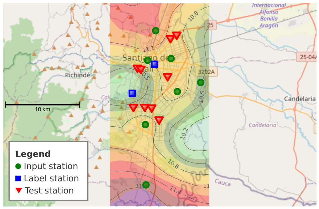
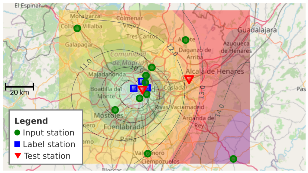
These data must be divided into the stations used as inputs and stations used as labels, and then they are randomly divided so that 80% of the samples are used for training and 20% for validation. Finally, the remaining sensors are used to test the trained nets, which are never exposed to these stations during training or validation and therefore represent virtually unmonitored locations from the model’s perspective. Madrid has 15 sensors that have been randomly divided into 10 input sensors, 3 label sensors, and 2 test sensors. For Cali, there are 9 sensors that provide reliable measurements, 7 of which have been randomly selected as inputs and the other 2 as labels. The remaining 9 sensors, which provided data with less frequency, were used for testing. The random partitioning of stations follows standard machine learning evaluation practices for estimating model performance [15,37] while avoiding manual selection bias. However, alternative validation schemes also exist for spatially structured data. For example, Alazmi and Rakha [38] compared random, spatial, and spatiotemporal cross-validation strategies and showed that random partitioning can lead to better apparent performance, whereas spatial partitioning avoids placing geographically close locations in both training and test sets. As a result, spatially blocked validation may provide a more stringent assessment when the goal is geographical extrapolation to unseen regions, while the random partition adopted here is intended to evaluate cross-location interpolation within the same urban domain. These stations are geographically represented in Figure 1 and Figure 2. To facilitate the academic community’s evaluation of the models against the results of this work, the dataset used has been published in Zenodo [33].

Madrid sits on Spain’s high central plateau with relatively open terrain. Urban traffic is the primary local source of air pollutants, while episodic Saharan dust intrusions can raise particulate levels (Dirección General de Sostenibilidad y Control Ambiental [39]). Cali lies on the Cauca River valley floor between Andean ranges. Local emissions are dominated by mobile sources, with seasonal regional biomass burning contributing to elevated particulate matter (Mateus-Fontecha et al. [40]). These geographic and source patterns frame the baseline concentrations and variability that are relevant to forecasting. Both cities are densely populated, with 3.5 and 2.3 million inhabitants, respectively. This work focuses on these cities because pollution poses a greater risk in densely populated areas where people and industry, making air quality monitoring more important. However, changes in model behavior may be expected in entirely different areas.

Figure 1. Cali monitoring stations and ${\mathrm{PM}}_{2.5}$ prediction for Cali. The heatmap delineates the study area and does not necessarily reflect officially recognized administrative boundaries. Map data from OpenStreetMap contributors [41]. Study area: $13.2\times 27.2$ km (359 ${\mathrm{km}}^2$).

Figure 1. Cali monitoring stations and ${\mathrm{PM}}_{2.5}$ prediction for Cali. The heatmap delineates the study area and does not necessarily reflect officially recognized administrative boundaries. Map data from OpenStreetMap contributors [41]. Study area: $13.2\times 27.2$ km (359 ${\mathrm{km}}^2$).

Figure 2. Madrid monitoring stations and ${\mathrm{PM}}_{10}$ prediction for Madrid. The heatmap delineates the study area and does not necessarily reflect officially recognized administrative boundaries. Map data from OpenStreetMap contributors [41]. Study area: $76.2\times 61.2$ km (4659 $\mathrm{km}$).

Figure 2. Madrid monitoring stations and ${\mathrm{PM}}_{10}$ prediction for Madrid. The heatmap delineates the study area and does not necessarily reflect officially recognized administrative boundaries. Map data from OpenStreetMap contributors [41]. Study area: $76.2\times 61.2$ km (4659 $\mathrm{km}$).

3.1. Data Preprocessing

Air quality monitoring systems are prone to data loss and corruption due to issues such as equipment failure, server connectivity problems, power outages, and other uncontrollable factors. Missing or erroneous values can adversely affect data mining and model performance. To mitigate these issues and optimize model training, we applied a series of preprocessing steps, as outlined below.

3.1.1. Data Collection

Initially, the data from each city was organized into separate files, with each record containing the following relevant features: timestamp, station identifier, latitude, longitude, temperature, humidity, dew point, and pollutant concentrations (${\mathrm{O}}_3$, ${\mathrm{NO}}_2$, ${\mathrm{PM}}_{2.5}$, ${\mathrm{PM}}_{10}$, CO, and ${\mathrm{SO}}_2$).

3.1.2. Outlier Removal

Invalid and extreme outlier values were identified and removed to ensure data quality. Records with pollutant values exceeding ${10}^{15}$ (likely artifacts caused by system errors) and negative values (physically implausible for pollutant concentrations) were excluded, accounting for approximately 0.1% of the total dataset. Subsequently, statistical outliers were removed using the interquartile range (IQR) method, where values falling outside three times the IQR for a given pollutant were considered outliers. A very small number of relative-humidity values slightly above 100% remained after preprocessing; these were retained because they were rare, close to the physical limit, and could not be confidently classified as erroneous without introducing an ad hoc filtering rule.

3.1.3. Data Aggregation

A manual inspection revealed that, while sensors typically reported data simultaneously, the sampling intervals varied, ranging from 15 min to over an hour. To standardize the data, timestamps were rounded to the nearest hour. Measurements were then aggregated by timestamp and station, computing the mean when multiple observations existed for the same hour and station. This step produced an evenly spaced temporal dataset and ensured the alignment of simultaneous measurements from different sensors.

Table 5. Records from Cali at 12:00 on 13 June 2024 after data aggregation. Each topic corresponds to a different station.

Timestamp	Topic	${\mathrm{O}}_3$	${\mathrm{NO}}_2$	${\mathrm{PM}}_{2.5}$	${\mathrm{PM}}_{10}$	CO	${\mathrm{SO}}_2$	Temp	Latitude	Longitude
13-06-2024 12:00:00	3318	19	7	14	32	540	1	17	3.457128	−76.502303
13-06-2024 12:00:00	3319	17	8	15	30	577	1	17	3.305339	−76.532581
13-06-2024 12:00:00	3320	19	7	14	32	540	1	17	3.450419	−76.522267
13-06-2024 12:00:00	3321	19	7	14	32	540	1	17	3.455469	−76.530992
13-06-2024 12:00:00	3322	17	7	16	31	577	1	17	3.490514	−76.521225
13-06-2024 12:00:00	3323	19	7	14	32	540	1	17	3.377911	−76.533811
13-06-2024 12:00:00	3324	18	6	11	28	563	1	17	3.417203	−76.494736
13-06-2024 12:00:00	3325	19	7	14	32	540	1	17	3.415389	−76.549347
13-06-2024 12:00:00	3326	18	6	11	28	563	1	17	3.428389	−76.466700

contains a data sample for a specific hour in Cali.

3.1.4. Handling Missing Values

Various strategies were considered to address missing values, including filling with the last observed value (Kalajdjieski et al. [17]), substituting zeros (Drewil and Al-Bahadili [4]), using the mean or median for each feature (Kumar and Pande [22]), and using splines (Bekkar et al. [5], Baniasadi et al. [7]). The advantages of these methods were discussed by Bougoudis et al. [13]. This paper evaluates and compares different approaches to determine the most suitable method for the given dataset. By default, missing values are discarded. These methods are detailed and analyzed in Section 3.4, and the most suitable method is selected. In any case, only the records used as inputs for the predictions were filled, never the labels.

3.1.5. Data Normalization

To facilitate model training and ensure consistent scaling across features, pollutant concentrations, meteorological variables, and distance were normalized to the $[0,1]$ range for each city, with normalization parameters computed on the training and validation data.

3.1.6. Time Window

As will be shown in Section 3.4, we chose not to impute all the missing values. As a result, the dataset does not contain continuous records for all the stations at all times. An analysis of the data revealed continuous periods of time when malfunction was common—likely due to hardware or software errors that were later corrected. To construct the samples, we used a rolling window approach, which requires a continuous sequence of records spanning the input window plus the target record. For every sample, we tested whether we had enough continuous data to fill the time window used for prediction and the predicted values. Only when no missing data was present in this time frame was the set of records added to the final dataset. The selected time window size is 24 h, meaning that if we want to make predictions for 1 h into the future, each sample requires 25 continuous hours of records.

3.1.7. Formatting

Each input sample contains the selected values from each station used as input plus the distance between said station and the point where we want to predict the pollutant calculated with the haversine formula. Although distance is time-invariant, it is included at each timestep of the input window together with the temporal features. This allows the model to process spatial and temporal information jointly in a unified input representation. For example, for Cali, where 7 stations are used as inputs, if we select 4 different features as inputs, the input size will be $7\times (4+1)=35$ for each timestamp, vectorized so that the order of the stations is always constant. Sorting the sensors in canonical order enables the model to recognize that each input originates from a particular station, learning the particular spatial characteristics that define each sensing location. The records from Table 5 have been formatted in

Table 6. Data from Cali at 12:00 on June 13th, 2024, after formatting relative to the label station with topic 3320 to predict the ${\mathrm{NO}}_2$. The topics are included as reference but they are not part of the input data. To create a valid sample, the data should be flattened, and 24 continuous records for all the input stations would be required.

(a) First hour of the input data
topic	${\mathbf{NO}}_2$	${\mathbf{PM}}_{2.5}$	${\mathbf{PM}}_{10}$	CO	distance
3318	0.2609	0.4194	0.4915	0.1824	0.0809
3319	0.3043	0.4516	0.4576	0.1970	1.0000
3321	0.2609	0.4194	0.4915	0.1824	0.0000
3322	0.2609	0.4839	0.4746	0.1970	0.2219
3323	0.2609	0.4194	0.4915	0.1824	0.4680
3324	0.2174	0.3226	0.4237	0.1915	0.2525
3326	0.2174	0.3226	0.4237	0.1915	0.3665
(b) Target data (12:00 on 14 June 2024 )
topic			${\mathbf{NO}}_2$
3320			0.3043

as part of a valid sample, where the selected features are ${\mathrm{NO}}_2$, ${\mathrm{PM}}_{2.5}$, ${\mathrm{PM}}_{10}$, and CO.

Importantly, this setting differs from conventional air quality time series forecasting: the objective is not to predict the next value of any monitored station’s time series, but to forecast the pollutant at a different target location. Thus, the predicted value does not belong to a time series directly observed by the model, which makes classical single-series approaches such as ARIMA/SARIMA (defined for a fixed, observed sequence) not directly applicable to this pipeline.

3.2. Feature Selection

A correlation-based feature selection technique was employed in this study to identify the optimal set of input variables to develop a predictive model. This method calculates the statistical correlation between each input variable and the target variable. Specifically, the Pearson correlation coefficient (which quantifies the linear relationship between two datasets) was used, similarly to the approach by Kristiani et al. [20]. Variables with the highest correlation to the target variable were selected for further analysis. To mitigate the effects of outliers and differences in scale, the correlation coefficients were computed after normalizing the data. Features with a Pearson correlation coefficient of at least 0.4 in a city were selected as inputs for the predictive model.

${\mathrm{O}}_3$ was predicted using ${\mathrm{O}}_3$, temperature, and dew point values. ${\mathrm{NO}}_2$ predictions relied on ${\mathrm{NO}}_2$, ${\mathrm{PM}}_{2.5}$, ${\mathrm{PM}}_{10}$, and CO. ${\mathrm{PM}}_{2.5}$ was predicted using ${\mathrm{NO}}_2$, ${\mathrm{PM}}_{2.5}$, and ${\mathrm{PM}}_{10}$. Finally, ${\mathrm{PM}}_{10}$ predictions used ${\mathrm{NO}}_2$, ${\mathrm{PM}}_{2.5}$, ${\mathrm{PM}}_{10}$, and CO as input variables.

3.3. Model Selection

The most suitable model for each prediction was identified among all the models described in Section 2. It had been hypothesized that not every pollutant or every time interval would achieve the best performance with the same model. To test this, a model was trained for each pollutant and time interval, and the RMSE in the validation set was compared. Each NN was trained with three different seeds, and we report the average performance across seeds.

Table A1. RMSE for the different models and pollutants for 1 h predictions. The minimum RMSE for each model, pollutant, and city is highlighted in bold.

	Cali				Madrid
Model	${\mathbf{O}}_{\mathbf{3}}$	${\mathbf{NO}}_{\mathbf{2}}$	${\mathbf{PM}}_{\mathbf{2.5}}$	${\mathbf{PM}}_{\mathbf{10}}$	${\mathbf{O}}_{\mathbf{3}}$	${\mathbf{NO}}_{\mathbf{2}}$	${\mathbf{PM}}_{\mathbf{2.5}}$	${\mathbf{PM}}_{\mathbf{10}}$
CNN	1.2039	0.8925	1.3999	1.96	1.087	2.5022	1.8221	3.391
GRU	1.3141	0.8921	1.3837	2.1615	1.2901	2.8796	1.99	3.4095
LSTM	1.2447	0.8567	1.4004	1.9401	1.01	2.7682	1.8479	2.9131
CNNLSTM	1.2871	0.8711	1.4518	2.1667	1.3295	2.5494	1.9086	3.355
CNNLSTMv2	1.2719	0.866	1.4384	2.2102	1.1813	2.5852	1.8657	3.2707
GRU×2	1.2905	0.8936	1.1419	1.9408	1.4894	2.7317	1.875	3.4037
LSTM×2	1.1465	0.8174	1.2152	1.7924	1.1198	2.3177	1.6235	2.8801
LSTMGRU	1.2293	0.8714	1.1946	1.7894	1.2133	2.6172	1.7618	3.1543
BiLSTM	1.3329	0.8622	1.3027	2.0922	1.3539	2.2598	1.8429	2.9069
RF	1.178	0.8445	1.3124	2.1286	1.867	3.7533	2.5496	4.1108
LR	1.4925	1.2579	1.5208	3.4354	4.0198	7.2151	5.1456	9.4336

,

Table A2. RMSE for the different models and pollutants for 2 h predictions. The minimum RMSE for each model, pollutant, and city is highlighted in bold.

	Cali				Madrid
Model	${\mathbf{O}}_{\mathbf{3}}$	${\mathbf{NO}}_{\mathbf{2}}$	${\mathbf{PM}}_{\mathbf{2.5}}$	${\mathbf{PM}}_{\mathbf{10}}$	${\mathbf{O}}_{\mathbf{3}}$	${\mathbf{NO}}_{\mathbf{2}}$	${\mathbf{PM}}_{\mathbf{2.5}}$	${\mathbf{PM}}_{\mathbf{10}}$
CNN	1.3109	0.9342	1.6075	2.2314	1.2026	2.7826	2.149	3.7321
GRU	1.4161	0.8713	1.5794	2.187	1.2593	3.1663	2.4183	3.4222
LSTM	1.2154	0.7806	1.3934	2.1267	0.9583	2.5025	2.084	3.3678
CNNLSTM	1.4978	1.0207	1.7834	2.3959	1.4756	2.915	2.177	3.9846
CNNLSTMv2	1.3893	0.9522	1.5963	2.5433	1.2425	2.7306	2.2377	3.8849
GRU×2	1.2782	0.7756	1.3901	1.8335	0.9712	2.7138	2.0523	3.4751
LSTM×2	1.054	0.7498	1.3088	1.8523	1.0034	2.4677	1.9225	3.3865
LSTMGRU	1.0521	0.7712	1.3705	1.8812	0.9558	2.7004	1.9778	3.2769
BiLSTM	1.5535	0.9898	1.3434	2.1394	1.0898	2.2952	2.0024	3.5099
RF	1.3038	0.9993	1.8988	2.2093	2.2627	4.3458	2.8024	4.7425
LR	1.9317	1.4412	2.0412	3.5733	4.3459	8.6068	5.9067	10.2099

,

Table A3. RMSE for the different models and pollutants for 1 d predictions. The minimum RMSE for each model, pollutant, and city is highlighted in bold.

	Cali				Madrid
Model	${\mathbf{O}}_{\mathbf{3}}$	${\mathbf{NO}}_{\mathbf{2}}$	${\mathbf{PM}}_{\mathbf{2.5}}$	${\mathbf{PM}}_{\mathbf{10}}$	${\mathbf{O}}_{\mathbf{3}}$	${\mathbf{NO}}_{\mathbf{2}}$	${\mathbf{PM}}_{\mathbf{2.5}}$	${\mathbf{PM}}_{\mathbf{10}}$
CNN	1.2175	0.9356	1.4553	2.1234	1.3571	3.4852	2.1707	4.1654
GRU	1.0934	0.8154	1.3282	1.9969	1.0525	2.7242	1.8595	3.6473
LSTM	1.0185	0.7906	1.2687	1.9765	1.0559	2.6357	2.0164	3.3138
CNNLSTM	1.1916	0.9889	1.5902	2.2644	1.7105	3.1138	2.4095	4.6035
CNNLSTMv2	1.1102	0.871	1.423	2.232	1.2622	3.1239	2.2386	4.2491
GRU×2	0.9879	0.786	1.0942	1.9243	1.1099	2.8283	1.6846	3.2495
LSTM×2	0.9741	0.8125	1.142	1.9435	1.1264	2.3738	1.693	3.1266
LSTMGRU	0.9661	0.7801	1.1728	1.9489	1.0289	2.5848	1.775	3.2459
BiLSTM	1.0262	0.8368	1.207	2.0096	1.2956	2.7192	1.8669	3.4451
RF	1.6229	1.0562	1.9765	2.7913	3.1193	5.4361	4.0779	7.1108
LR	3.0511	2.2773	2.8992	5.643	5.2102	10.4549	9.4148	11.8843

,

Table A4. RMSE for the different models and pollutants for 4 d predictions. The minimum RMSE for each model, pollutant, and city is highlighted in bold.

	Cali				Madrid
Model	${\mathbf{O}}_{\mathbf{3}}$	${\mathbf{NO}}_{\mathbf{2}}$	${\mathbf{PM}}_{\mathbf{2.5}}$	${\mathbf{PM}}_{\mathbf{10}}$	${\mathbf{O}}_{\mathbf{3}}$	${\mathbf{NO}}_{\mathbf{2}}$	${\mathbf{PM}}_{\mathbf{2.5}}$	${\mathbf{PM}}_{\mathbf{10}}$
CNN	1.4067	0.8932	1.641	2.9884	2.5931	2.6143	1.6056	2.9405
GRU	1.2901	0.7994	1.3989	2.2654	2.1539	2.2355	1.4883	2.9765
LSTM	1.1958	0.7463	1.3858	2.2262	2.2531	2.9547	1.499	3.0553
CNNLSTM	1.9609	0.9562	1.7787	2.9198	2.1227	2.6608	1.851	3.2276
CNNLSTMv2	1.449	0.8728	1.5471	2.4217	2.3781	2.6221	1.4765	3.0223
GRU×2	1.2191	0.7382	1.2061	2.2737	1.5717	2.16	1.4289	3.0113
LSTM×2	1.155	0.7365	1.3129	2.2151	2.6031	2.2951	1.3925	2.8596
LSTMGRU	1.1922	0.7119	1.228	2.1587	1.9391	2.2764	1.4727	2.8436
BiLSTM	1.5679	0.8026	1.3454	2.392	2.5088	2.3214	1.4131	3.0261
RF	1.5738	1.1043	1.7435	2.9649	3.315	4.8808	4.159	5.7669
LR	3.0989	2.5403	3.0175	6.0211	5.7519	6.0826	4.7668	7.6473

,

Table A5. RMSE for the different models and pollutants for 7 d predictions. The minimum RMSE for each model, pollutant, and city is highlighted in bold.

	Cali				Madrid
Model	${\mathbf{O}}_{\mathbf{3}}$	${\mathbf{NO}}_{\mathbf{2}}$	${\mathbf{PM}}_{\mathbf{2.5}}$	${\mathbf{PM}}_{\mathbf{10}}$	${\mathbf{O}}_{\mathbf{3}}$	${\mathbf{NO}}_{\mathbf{2}}$	${\mathbf{PM}}_{\mathbf{2.5}}$	${\mathbf{PM}}_{\mathbf{10}}$
CNN	1.2713	0.8414	1.5152	2.1769	1.7253	2.8943	1.998	3.8344
GRU	1.0779	0.7628	1.2256	1.976	1.4386	2.6969	1.7406	3.4644
LSTM	0.9995	0.7586	1.2388	1.8854	1.3188	2.4453	1.7092	3.3163
CNNLSTM	1.744	0.9592	1.5268	2.5446	2.3521	2.7419	1.8371	3.6323
CNNLSTMv2	1.3136	0.8299	1.3551	2.0823	1.9047	2.7334	1.8444	3.6965
GRU×2	1.0647	0.6957	1.0884	1.7376	1.3641	2.6461	1.6052	3.1971
LSTM×2	0.9776	0.767	1.0712	1.8767	1.2424	2.3805	1.724	3.3236
LSTMGRU	0.9728	0.7179	1.1513	1.6641	1.3618	2.7968	1.7096	3.3772
BiLSTM	1.2819	0.7779	1.2184	2.0468	1.6015	2.5838	1.834	3.6497
RF	1.3302	1.0126	1.5767	2.272	3.9174	4.7175	3.5332	5.2129
LR	2.646	2.8134	2.9109	5.4209	3.4958	6.6931	6.544	10.3443

, and

Table A6. RMSE for the different models and pollutants for 10 d predictions. The minimum RMSE for each model, pollutant, and city is highlighted in bold.

	Cali				Madrid
Model	${\mathbf{O}}_{\mathbf{3}}$	${\mathbf{NO}}_{\mathbf{2}}$	${\mathbf{PM}}_{\mathbf{2.5}}$	${\mathbf{PM}}_{\mathbf{10}}$	${\mathbf{O}}_{\mathbf{3}}$	${\mathbf{NO}}_{\mathbf{2}}$	${\mathbf{PM}}_{\mathbf{2.5}}$	${\mathbf{PM}}_{\mathbf{10}}$
CNN	1.306	0.8122	1.4415	3.6407	1.2092	2.7345	2.0246	3.5158
GRU	1.169	0.6916	1.3018	3.1732	1.1045	2.2539	1.6438	2.9325
LSTM	1.1612	0.6999	1.2695	3.0594	1.1928	2.2065	1.6853	2.7058
CNNLSTM	1.7012	0.9429	1.789	3.4569	1.4461	2.9656	1.8623	3.421
CNNLSTMv2	1.3979	0.8153	1.5966	3.3839	1.3618	2.768	1.8114	3.4916
GRU×2	1.1699	0.653	1.1288	3.1214	1.225	2.3017	1.5738	3.0261
LSTM×2	1.1803	0.6787	1.2201	3.0115	1.0709	2.2416	1.5576	2.9261
LSTMGRU	1.1292	0.673	1.2074	3.1382	1.1165	2.3939	1.7115	2.9512
BiLSTM	1.2968	0.7113	1.2182	3.0347	1.2936	2.2491	1.7714	2.9301
RF	1.5748	0.9447	1.7455	3.6263	2.169	4.6285	3.1397	4.6607
LR	2.944	3.2729	3.5946	6.9411	2.8422	6.9599	4.258	5.5772

, respectively, corresponding to the analyzed time intervals (1 h, 2 h, 1 d, 4 d, 7 d, and 10 d), contain the mean RMSE obtained in the validation set when no imputation technique was used for every target pollutant, model, and city. The methods that minimized the mean RMSE in the validation set were selected for each pollutant, time horizon, and city. The models that have been selected are indicated in bold in Table A1, Table A2, Table A3, Table A4, Table A5 and Table A6. The tables also contain RMSE values for a LR model and a RF regressor with 100 trees. This allows for the contextualization of the improvement achieved by deep learning.

3.4. Imputation Technique Selection

As discussed earlier, this study explores different strategies for handling missing data, each of which impacts the final dataset size. The first strategy involves excluding all records with missing values. The second strategy fills gaps of up to one hour using the last available value from the same sensor; however, gaps exceeding one hour remain unfilled. The third strategy builds on the second by imputing any remaining missing values with the mean or median pollutant concentration, but only for timestamps where at least half of the sensors provided valid data. If not enough valid records were available for a particular timestamp, this imputation strategy was not performed for that timestamp. Finally, the last strategy, which is the most aggressive, uses the traditional approach of imputing all missing values with the mean. The application of these imputation techniques was exclusive to records from input stations and not to target labels.

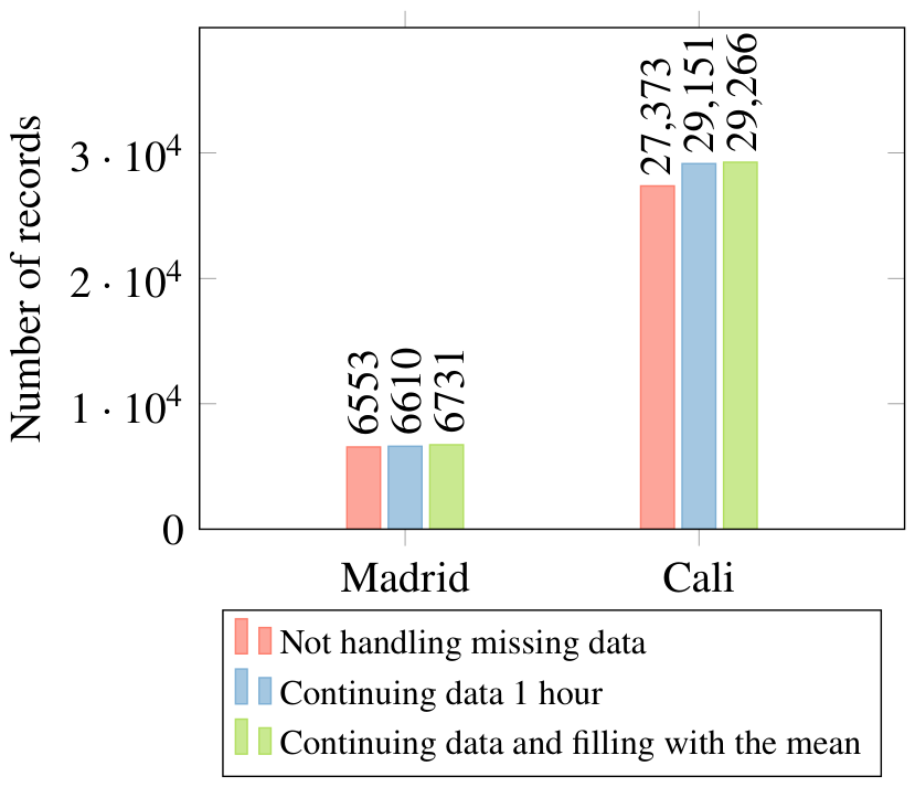
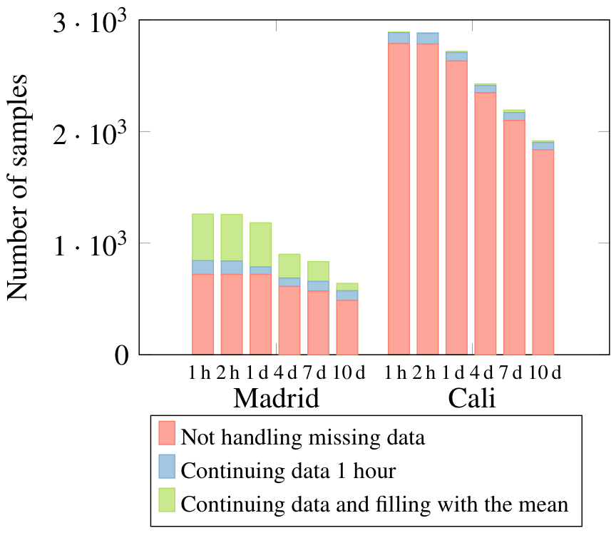
Figure 3 provides an overview of the number of valid records retained per city after applying each missing value handling technique, not counting any record with missing values. To account for time window constraints, Figure 4 illustrates the number of samples available for each dataset after the preprocessing steps described in Section 3.1.6. For each city, datasets are presented for six prediction horizons: one hour, two hours, one day, four days, seven days, and ten days into the future.

For the selected features and models, three distinct neural networks were trained for each of the approaches described for handling missing values. The method that minimized the mean RMSE in the validation set was chosen for each city. The selected imputation techniques have been marked in bold in

Table A7. RMSE for the different imputation techniques and pollutants for all the time lag predictions. The minimum RMSE for each imputation technique, pollutant, and city is highlighted in bold.

Time	Imputation	Cali				Madrid
Lag	Technique	${\mathbf{O}}_{\mathbf{3}}$	${\mathbf{NO}}_{\mathbf{2}}$	${\mathbf{PM}}_{\mathbf{2.5}}$	${\mathbf{PM}}_{\mathbf{10}}$	${\mathbf{O}}_{\mathbf{3}}$	${\mathbf{NO}}_{\mathbf{2}}$	${\mathbf{PM}}_{\mathbf{2.5}}$	${\mathbf{PM}}_{\mathbf{10}}$
1 h	None	1.1465	0.8174	1.1419	1.7894	1.0100	2.2598	1.6235	2.8801
	Continuity	1.1242	0.8839	1.4799	2.4818	1.2020	2.5830	1.6763	2.7969
	Mean	1.2888	0.9035	1.2770	2.3411	1.2913	2.5314	1.8047	3.5056
	Median	1.3005	0.9328	1.4672	1.9912	1.3778	2.4685	1.5649	2.8882
	Traditional	1.2671	0.8804	1.3031	2.4707	1.3893	2.5314	1.8015	3.5213
2 h	None	1.0521	0.7498	1.3088	1.8335	0.9558	2.2952	1.9225	3.2769
	Continuity	1.2556	0.7770	1.3379	2.2766	1.3211	2.1756	1.4803	3.2297
	Mean	1.1717	0.7793	1.3090	2.4934	1.2033	2.4351	1.5846	2.8608
	Median	1.1128	0.7703	1.2001	1.8018	1.0956	2.4628	1.6197	3.1134
	Traditional	1.2062	0.8333	1.2283	2.1201	1.1771	2.4351	1.5613	2.9488
1 d	None	0.9741	0.7801	1.0942	1.9243	1.0289	2.3738	1.6846	3.1266
	Continuity	1.0534	0.9430	1.2747	2.2844	2.0490	2.5120	1.8295	2.9310
	Mean	1.0522	0.7711	1.3387	2.1877	1.0392	2.3857	1.6387	2.8488
	Median	1.0147	0.7211	1.2820	1.7101	1.1036	2.4836	1.6538	2.6917
	Traditional	1.0203	0.7465	1.3395	2.9801	1.1440	2.3857	1.6539	2.9936
4 d	None	1.1550	0.7119	1.2061	2.1587	1.5717	2.1600	1.3925	2.8436
	Continuity	1.1064	0.7240	1.0634	2.1289	1.3873	2.5623	1.8294	3.7501
	Mean	1.1116	0.7742	1.3709	2.3013	1.2476	2.3646	1.9425	2.9230
	Median	1.1205	0.7778	1.3669	2.4201	1.2490	2.3646	1.9425	2.9230
	Traditional	1.0988	0.7681	1.3813	2.3821	1.2393	2.3646	1.9425	2.9230
7 d	None	0.9728	0.6957	1.0712	1.6641	1.2424	2.3805	1.6052	3.1971
	Continuity	1.5562	0.7868	1.2907	2.5670	1.3632	2.6311	2.2223	3.6341
	Mean	1.4458	0.7438	1.4008	2.8037	1.0924	2.5194	1.7606	3.0882
	Median	1.4543	0.7331	1.4425	2.9065	1.0958	2.5194	1.7606	3.0882
	Traditional	1.4541	0.7677	1.4056	2.8614	1.1524	2.5194	1.7606	3.0882
10 d	None	1.1292	0.6530	1.1288	3.0115	1.0709	2.2065	1.5576	2.7058
	Continuity	1.0967	0.7786	1.2308	2.4400	1.8810	2.2596	1.4999	2.4970
	Mean	1.1619	0.8427	1.2866	2.3458	1.5717	2.0215	1.3598	2.5251
	Median	1.1304	0.8225	1.2870	2.3540	1.5354	2.0215	1.3598	2.5251
	Traditional	1.1923	0.8464	1.2845	2.3887	1.5463	2.0215	1.3598	2.5251

.

In an operational deployment, the framework can be configured to prioritize either forecast continuity or forecast reliability. In the present study, we adopt a reliability-oriented setting in which the model is updated only when the inference input satisfies the same completeness requirements used during training. This choice is motivated by the fact that, as will be shown in the Results section, once a valid input window can be constructed, the proposed framework is highly resilient to random missing values: even when a substantial fraction of the input variables is replaced by feature-wise mean values, the increase in prediction error remains moderate. However, real-world outages rarely occur as isolated missing values. In practice, sensor failures or communication problems usually produce structured gaps over extended periods, which may remove the data of multiple stations for longer than the 24-h sliding window and therefore reduce the available spatial information. Under these conditions, a more aggressive imputation strategy could still be applied to force prediction generation, but our results show that such approaches may substantially degrade predictive accuracy. For this reason, when the available data are insufficient to support a reliable update, the framework can instead rely on previously generated longer-horizon forecasts, whose expected error is already characterized. This design reflects a deliberate operational trade-off between heatmap continuity and forecast trustworthiness in sparse and imperfect sensing environments.

4. Results

This section presents the results of our proposed deep learning modeling framework for air quality forecasting, focusing on model selection and imputation strategies. We report performance across different pollutants, cities, and prediction horizons, evaluating the models using different metrics. RMSE is reported in this section, while the rest of the metrics (${\mathrm{R}}^2$, mean absolute error (MAE), symmetric mean absolute percentage error (SMAPE), and mean bias error (MBE)) are provided in Appendix B. The outcomes are analyzed to highlight the improvements achieved through optimal model configuration and data preprocessing.

To contextualize the results presented in this section, we first report the RMSE obtained using a simple non-learning baseline in

Table 7. Root mean squared error (RMSE) obtained using the non-learning baseline (naïve temporal forecast combined with nearest-neighbor spatial assignment) for each pollutant, city, and forecast horizon.

Time	Cali				Madrid
Lag	${\mathbf{O}}_{\mathbf{3}}$	${\mathbf{NO}}_{\mathbf{2}}$	${\mathbf{PM}}_{\mathbf{2.5}}$	${\mathbf{PM}}_{\mathbf{10}}$	${\mathbf{O}}_{\mathbf{3}}$	${\mathbf{NO}}_{\mathbf{2}}$	${\mathbf{PM}}_{\mathbf{2.5}}$	${\mathbf{PM}}_{\mathbf{10}}$
1 h	1.7704	1.1223	2.4704	5.0467	5.7780	5.0080	4.6582	9.1177
2 h	2.3398	1.4913	2.9197	5.6293	6.0605	6.2456	4.9524	9.6034
1 d	3.6900	2.5715	4.1155	7.7785	6.7663	8.5737	8.0374	13.1741
4 d	5.2120	3.1284	4.6061	9.4008	8.1148	9.7656	10.5644	18.7440
7 d	6.3635	3.5200	4.5318	9.1421	9.4023	10.6264	11.6571	20.8573
10 d	7.5202	4.1624	5.3897	10.8948	10.3191	11.7324	13.5531	24.2929

. This baseline combines a naïve temporal forecast (assuming that the value at the target time is equal to the most recent observed value) and a nearest-neighbor spatial approximation (assigning to each location the value measured at the closest monitoring station). This baseline provides a practical reference point for evaluating the error reduction achieved by the proposed models relative to a simple continuity-based assumption. Compared with global statistical descriptors such as the standard deviation, this approach offers a more realistic benchmark because it explicitly accounts for both temporal persistence and spatial proximity. From these results, it can be observed that pollutant concentrations in Madrid exhibit higher variability than in Cali, which implies that all models, including the proposed deep learning approaches, are expected to face a more challenging prediction task in Madrid.

4.1. Model and Imputation Technique Selection

Table 8. RMSE for the selected models in the validation set.

Time	Cali				Madrid
Lag	${\mathbf{O}}_{\mathbf{3}}$	${\mathbf{NO}}_{\mathbf{2}}$	${\mathbf{PM}}_{\mathbf{2.5}}$	${\mathbf{PM}}_{\mathbf{10}}$	${\mathbf{O}}_{\mathbf{3}}$	${\mathbf{NO}}_{\mathbf{2}}$	${\mathbf{PM}}_{\mathbf{2.5}}$	${\mathbf{PM}}_{\mathbf{10}}$
1 h	1.1242	0.8174	1.1419	1.7894	1.0100	2.2598	1.5649	2.7969
2 h	1.0521	0.7498	1.2001	1.8018	0.9558	2.1756	1.4803	2.8608
1 d	0.9741	0.7211	1.0942	1.7101	1.0289	2.3738	1.6387	2.6917
4 d	1.0988	0.7119	1.0634	2.1289	1.2393	2.1600	1.3925	2.8436
7 d	0.9728	0.6957	1.0712	1.6641	1.0924	2.3805	1.6052	3.0882
10 d	1.0967	0.6530	1.1288	2.3458	1.0709	2.0215	1.3598	2.4970

contains the RMSE for the selected models, and

Table A8. ${\mathrm{R}}^2$ for the selected models in the validation set.

Time	Cali				Madrid
Lag	${\mathbf{O}}_{\mathbf{3}}$	${\mathbf{NO}}_{\mathbf{2}}$	${\mathbf{PM}}_{\mathbf{2.5}}$	${\mathbf{PM}}_{\mathbf{10}}$	${\mathbf{O}}_{\mathbf{3}}$	${\mathbf{NO}}_{\mathbf{2}}$	${\mathbf{PM}}_{\mathbf{2.5}}$	${\mathbf{PM}}_{\mathbf{10}}$
1 h	0.9265	0.9191	0.8337	0.8829	0.9594	0.9434	0.9526	0.9498
2 h	0.9293	0.9292	0.8416	0.8957	0.9633	0.9389	0.9463	0.9527
1 d	0.9449	0.9464	0.8682	0.9176	0.9484	0.9409	0.9461	0.9594
4 d	0.9174	0.9403	0.8410	0.7894	0.9473	0.9474	0.9642	0.9554
7 d	0.9236	0.9319	0.8152	0.8551	0.9566	0.8984	0.9502	0.9167
10 d	0.9108	0.9354	0.8411	0.8351	0.9528	0.9271	0.9679	0.9441

,

Table A9. Mean absolute error (MAE) for the selected models in the validation set.

Time	Cali				Madrid
Lag	${\mathbf{O}}_{\mathbf{3}}$	${\mathbf{NO}}_{\mathbf{2}}$	${\mathbf{PM}}_{\mathbf{2.5}}$	${\mathbf{PM}}_{\mathbf{10}}$	${\mathbf{O}}_{\mathbf{3}}$	${\mathbf{NO}}_{\mathbf{2}}$	${\mathbf{PM}}_{\mathbf{2.5}}$	${\mathbf{PM}}_{\mathbf{10}}$
1 h	0.8200	0.5431	0.8216	1.2744	0.7917	1.7702	1.1375	2.0367
2 h	0.7876	0.5155	0.8250	1.2642	0.7212	1.6840	1.1197	2.1317
1 d	0.7316	0.5014	0.7588	1.1894	0.7592	1.8626	1.1847	1.9419
4 d	0.8028	0.4886	0.7560	1.4263	0.9184	1.5927	1.0804	2.0428
7 d	0.7334	0.4768	0.7638	1.1064	0.8157	1.7575	1.1764	2.2831
10 d	0.7920	0.4730	0.7729	1.5794	0.8060	1.4455	0.9342	1.8480

,

Table A10. Symmetric mean absolute percentage error (SMAPE) for the selected models in the validation set.

Time	Cali				Madrid
Lag	${\mathbf{O}}_{\mathbf{3}}$	${\mathbf{NO}}_{\mathbf{2}}$	${\mathbf{PM}}_{\mathbf{2.5}}$	${\mathbf{PM}}_{\mathbf{10}}$	${\mathbf{O}}_{\mathbf{3}}$	${\mathbf{NO}}_{\mathbf{2}}$	${\mathbf{PM}}_{\mathbf{2.5}}$	${\mathbf{PM}}_{\mathbf{10}}$
1 h	6.503	3.994	3.999	3.664	8.712	10.204	12.469	9.441
2 h	6.584	4.047	6.253	4.622	7.645	10.270	12.519	11.011
1 d	6.099	5.753	4.984	4.382	8.177	10.721	12.802	10.713
4 d	6.099	4.912	5.538	4.940	8.421	12.008	13.827	11.742
7 d	5.540	4.779	5.423	3.685	7.182	14.066	18.019	13.923
10 d	6.242	4.686	5.308	5.285	6.673	10.911	13.964	12.463

and

Table A11. Mean bias error (MBE) for the selected models in the validation set.

Time	Cali				Madrid
Lag	${\mathbf{O}}_{\mathbf{3}}$	${\mathbf{NO}}_{\mathbf{2}}$	${\mathbf{PM}}_{\mathbf{2.5}}$	${\mathbf{PM}}_{\mathbf{10}}$	${\mathbf{O}}_{\mathbf{3}}$	${\mathbf{NO}}_{\mathbf{2}}$	${\mathbf{PM}}_{\mathbf{2.5}}$	${\mathbf{PM}}_{\mathbf{10}}$
1 h	−0.0216	−0.0008	−0.0470	0.0640	−0.0361	−0.0096	0.0296	−0.0098
2 h	−0.0322	0.0969	−0.0727	0.0847	−0.0482	−0.0716	0.0244	0.1088
1 d	0.0241	−0.0703	−0.0157	−0.1419	−0.0701	−0.0990	0.0497	0.1317
4 d	−0.0017	0.0152	−0.0042	0.0556	0.0186	−0.1402	0.1548	0.2494
7 d	0.0094	−0.0401	−0.0680	0.0264	−0.0587	0.2217	−0.2138	−0.1615
10 d	−0.0501	0.0258	−0.0381	0.1673	−0.0874	0.2023	0.1784	0.1414

contain additional metrics for said models. In terms of ${\mathrm{R}}^2$, ${\mathrm{PM}}_{2.5}$ shows the worst performance (on average, 0.8973) whereas ${\mathrm{PM}}_{10}$ shows the worst RMSE (on average, $2.3515$ $\mathrm{\mu }\mathrm{g} {\mathrm{m}}^{-3}$) due to the greater variability of this pollutant. Note that since the precision of all the input parameters is one unit, arguably, an error of less than one should not be relevant. A real inference scenario is illustrated in Figure 1 and Figure 2, which also show the location of the monitoring stations and the area of study.

We have observed that selecting the optimal model and imputation technique is a choice that depends on the time lag, the pollutant being predicted, and the city where it is being applied. Out of all the models considered in the 48 cases shown in Table A1, Table A2, Table A3, Table A4, Table A5 and Table A6, LSTM was selected 3 times, GRU×2 13 times, LSTM×2 18 times, LSTMGRU 12 times, and BiLSTM twice. Despite CNN’s great ability to recognize patterns, its performance is not as good as models specifically designed for time series. Likewise, neither version of MCNNLSTM was the best option for any of the analyzed cases, and GRU, RF, and LR were possibly too simple for the problem at hand, as we can see a clear dominance of models with two recursive layers. Interestingly, the dominance of LSTM×2 for 1-hour forecasting is notable, whereas for longer time lags, GRU×2 and LSTMGRU offer comparable results. For Cali predictions, there is no significant difference between these three models with two recursive layers, whereas in Madrid, we see a dominance of the LSTM×2 model. Baseline models (RF and LR) fail to offer meaningful predictions, especially for Madrid, which has a smaller dataset. They lead to a 72.5% and 203.1% increase in RMSE compared to the optimal choice, respectively. For Cali, they perform better, but still undoubtedly worse that the DL architectures proposed.

The comparison of model architectures can be interpreted as an ablation study on temporal depth and architectural composition. Single-layer recurrent models (GRU, LSTM) capture short-term dependencies, whereas two-layer recurrent architectures (GRU×2, LSTM×2, LSTMGRU) provide a hierarchical temporal representation that consistently yields better performance across pollutants and forecasting horizons, indicating the presence of multi-scale temporal dynamics in air quality time series. In contrast, although the multipath models combine CNN and LSTM branches and can be viewed as an ablation of complementary feature extractors (capturing local temporal patterns and sequential dependencies) their joint representation does not translate into superior performance, as they are never selected as the best-performing models. This result is consistent with the observed behavior of the standalone CNN models, which also fail to outperform recurrent architectures in this framework. This suggests that the extraction of temporal dependencies is more effectively handled by recurrent structures than by convolutional layers in this setting. Overall, these findings indicate that increasing temporal depth within recurrent networks is more beneficial than combining heterogeneous branches, highlighting the dominant role of hierarchical temporal modeling over architectural diversity for this task.

Regarding the imputation technique, our results show that in most cases the optimal strategy is to discard missing values rather than indiscriminately replacing them with the mean or median. This finding indicates that data quality is more critical than data quantity: a smaller but more reliable dataset can yield better predictive performance than a larger dataset contaminated by poorly imputed values. Consequently, traditional imputation strategies that do not account for data availability or reliability may degrade model performance. As shown in Table A7, the most severe degradation due to traditional imputation occurred for Cali ${\mathrm{PM}}_{10}$ forecasting with a 1-day time lag, where the RMSE increased by 74.3% relative to the optimal configuration.

For Madrid (where, as discussed in Section 3.4, the dataset was smaller but highly reliable, with 82.7% of valid records), we found that for more than half of the scenarios, the best approach was to discard the missing values or apply continuity for one hour. For Cali, with merely 30.5% of valid records, no imputation was usually the best approach, with the traditional approach performing better only once. In general, the enhancement achieved by joint model optimization and imputation technique selection is substantial: deviations from the best configuration resulted in RMSE increases ranging from 14.1% to 115.3%. On average, our optimized approach outperformed the worst DL model by 37.9% (by 203.8% if considering RF and LR) and the worst imputation strategy by 26.6% across all cities, pollutants, and time intervals, amounting to an average improvement of 48.9%.

By analyzing autocorrelation at a 24-h lag, we assess the strength of the daily periodicity for each pollutant across different topics. The different imputation strategies have little impact on variables that already exhibit a strong 24-h cycle, such as temperature and ozone, indicating that their intrinsic daily structure is robust to missing-data handling. In contrast, pollutants with weaker inherent periodicity are more sensitive to the imputation method, with CO being the most affected, showing a noticeable reduction in its 24-h autocorrelation. These results are consistent with the previously observed behavior: ${\mathrm{PM}}_{10}$ exhibits the most significant degradation when using the most aggressive imputation, and it is also the only pollutant that uses CO as an input feature. This suggests that the loss of temporal structure in CO propagates through the modeling pipeline and contributes to the reduced performance of ${\mathrm{PM}}_{10}$ forecasting.

4.2. Evaluation on Unobserved Monitoring Sites

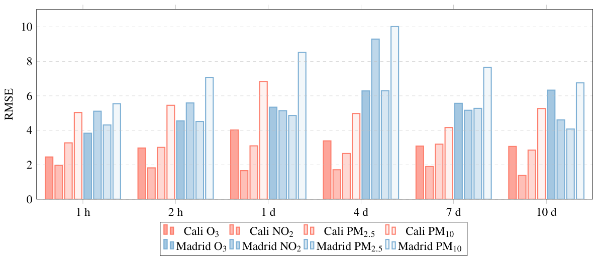
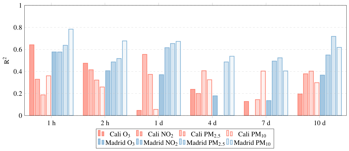
To assess the accuracy of our model in predicting pollution levels across the city, we have evaluated the performance of our trained model compared to locations that were not used during the training process. Specifically, the levels of the four pollutants (${\mathrm{O}}_3$, ${\mathrm{NO}}_2$, ${\mathrm{PM}}_{2.5}$, and ${\mathrm{PM}}_{10}$) were inferred by the test sensors. The results are presented in

Table 9. RMSE obtained on sensors not used during training or validation, reported for each city, pollutant, and forecast horizon.

Time	Cali				Madrid
Lag	${\mathbf{O}}_{\mathbf{3}}$	${\mathbf{NO}}_{\mathbf{2}}$	${\mathbf{PM}}_{\mathbf{2.5}}$	${\mathbf{PM}}_{\mathbf{10}}$	${\mathbf{O}}_{\mathbf{3}}$	${\mathbf{NO}}_{\mathbf{2}}$	${\mathbf{PM}}_{\mathbf{2.5}}$	${\mathbf{PM}}_{\mathbf{10}}$
1 h	3.0298	1.9648	3.2708	5.0318	3.6402	5.1061	4.3098	5.5432
2 h	3.5730	1.8176	3.0075	5.4495	3.9959	5.5853	4.5108	7.0737
1 d	2.7969	1.6541	3.0965	6.8332	3.6611	5.1383	4.8580	8.5248
4 d	3.2995	1.7079	2.6518	4.9726	5.8129	9.2936	6.2921	10.0208
7 d	3.2743	1.8956	3.1945	4.1578	4.8944	5.1605	5.2703	7.6586
10 d	2.9887	1.3795	2.8521	5.2637	5.5041	4.6047	4.0748	6.7517

, which shows the RMSE, and in

Table A12. ${\mathrm{R}}^2$ obtained on sensors not used during training or validation, reported for each city, pollutant, and forecast horizon.

Time	Cali				Madrid
Lag	${\mathbf{O}}_{\mathbf{3}}$	${\mathbf{NO}}_{\mathbf{2}}$	${\mathbf{PM}}_{\mathbf{2.5}}$	${\mathbf{PM}}_{\mathbf{10}}$	${\mathbf{O}}_{\mathbf{3}}$	${\mathbf{NO}}_{\mathbf{2}}$	${\mathbf{PM}}_{\mathbf{2.5}}$	${\mathbf{PM}}_{\mathbf{10}}$
1 h	0.4404	0.3293	0.1875	0.3604	0.4754	0.5765	0.6376	0.7839
2 h	0.2391	0.4151	0.3218	0.2588	0.3690	0.4862	0.5173	0.6771
1 d	0.5353	0.5547	0.3734	0.0554	0.3630	0.6157	0.6533	0.6729
4 d	0.2815	0.2001	0.4065	0.3247	0.3357	−0.4128	0.4862	0.5380
7 d	0.0145	-0.0179	0.1443	0.4035	0.2908	0.4941	0.5237	0.4046
10 d	0.2276	0.3785	0.4029	0.2980	0.3813	0.5493	0.7182	0.6183

,

Table A13. MAE obtained on sensors not used during training or validation, reported for each city, pollutant, and forecast horizon.

Time	Cali				Madrid
Lag	${\mathbf{O}}_{\mathbf{3}}$	${\mathbf{NO}}_{\mathbf{2}}$	${\mathbf{PM}}_{\mathbf{2.5}}$	${\mathbf{PM}}_{\mathbf{10}}$	${\mathbf{O}}_{\mathbf{3}}$	${\mathbf{NO}}_{\mathbf{2}}$	${\mathbf{PM}}_{\mathbf{2.5}}$	${\mathbf{PM}}_{\mathbf{10}}$
1 h	2.0901	1.4390	2.3726	3.6859	2.9536	4.0873	2.9916	4.0185
2 h	2.5289	1.3028	2.2080	3.9111	3.0224	4.3905	3.2168	5.2167
1 d	1.8821	1.1905	2.2133	4.5267	2.7648	3.8664	3.1720	5.9992
4 d	2.3218	1.2079	1.9337	3.5868	4.3507	6.5325	3.9852	6.6443
7 d	2.3858	1.3394	2.3642	2.9345	3.8896	4.0409	3.6068	5.5443
10 d	2.1064	1.0172	2.0348	3.7471	4.6871	3.6059	2.7128	4.8748

,

Table A14. SMAPE obtained on sensors not used during training or validation, reported for each city, pollutant, and forecast horizon.

Time	Cali				Madrid
Lag	${\mathbf{O}}_{\mathbf{3}}$	${\mathbf{NO}}_{\mathbf{2}}$	${\mathbf{PM}}_{\mathbf{2.5}}$	${\mathbf{PM}}_{\mathbf{10}}$	${\mathbf{O}}_{\mathbf{3}}$	${\mathbf{NO}}_{\mathbf{2}}$	${\mathbf{PM}}_{\mathbf{2.5}}$	${\mathbf{PM}}_{\mathbf{10}}$
1 h	20.698	13.154	17.076	12.216	30.805	26.937	26.849	17.151
2 h	23.661	12.014	15.169	13.283	30.269	27.991	26.979	23.544
1 d	17.661	10.874	16.023	16.417	29.674	25.677	27.809	26.753
4 d	18.900	10.351	12.517	10.858	36.464	41.236	34.061	29.941
7 d	20.217	11.800	15.122	8.973	35.169	27.565	33.248	26.752
10 d	17.722	8.833	12.846	10.873	41.587	28.000	28.558	26.689

and

Table A15. MBE obtained on sensors not used during training or validation, reported for each city, pollutant, and forecast horizon.

Time	Cali				Madrid
Lag	${\mathbf{O}}_{\mathbf{3}}$	${\mathbf{NO}}_{\mathbf{2}}$	${\mathbf{PM}}_{\mathbf{2.5}}$	${\mathbf{PM}}_{\mathbf{10}}$	${\mathbf{O}}_{\mathbf{3}}$	${\mathbf{NO}}_{\mathbf{2}}$	${\mathbf{PM}}_{\mathbf{2.5}}$	${\mathbf{PM}}_{\mathbf{10}}$
1 h	−0.2479	0.2492	1.0397	2.1091	−1.1692	−3.6888	−0.0859	0.0865
2 h	−0.4733	0.2996	0.8459	2.1141	−1.0748	−3.6533	−0.0798	−0.6240
1 d	0.1329	0.0866	0.9692	2.8085	−1.2121	−2.5023	1.5142	2.1311
4 d	−0.8281	0.1062	0.8312	1.9758	−0.2806	−6.0440	2.4777	4.6540
7 d	−0.8650	0.2901	0.7572	1.6696	−2.4089	−2.1115	−0.5603	0.6276
10 d	−0.7602	0.2218	0.9962	1.8758	−2.3824	−1.3352	1.0333	0.8731

, which show the rest of the metrics. RMSE and ${\mathrm{R}}^2$ are graphically represented in Figure 5 and Figure 6. As expected, performance was worse when tested against new locations than when tested against the validation set. Nevertheless, the results are still promising, with an average RMSE of $3.87$ ppb for ${\mathrm{O}}_3$, $3.78$ ppb for ${\mathrm{NO}}_2$, $3.95$ $\mathrm{\mu }\mathrm{g} {\mathrm{m}}^{-3}$ for ${\mathrm{PM}}_{2.5}$, and $6.44$ $\mathrm{\mu }\mathrm{g} {\mathrm{m}}^{-3}$ for ${\mathrm{PM}}_{10}$. The models, which were initially developed for short-term forecasting (up to one day), exhibit anomalous behavior in a few extended-period scenarios, as evidenced by negative ${\mathrm{R}}^2$ values in two scenarios.Negative ${\mathrm{R}}^2$ values indicate that, in those scenarios, the model performed worse than a constant predictor equal to the mean of the target variable. This is likely attributable to an inability to adequately capture long-term anthropogenic pollution sources, a deficiency that could be addressed by expanding the time frame under consideration and incorporating additional inputs, such as the day of the week.

This finding aligns with the conclusions drawn from prior studies, which indicate that a longer time lag does not necessarily equate with a decline in prediction accuracy. For ${\mathrm{NO}}_2$, the optimal results are attained for the extended 1-day time lag, whereas ${\mathrm{O}}_3$ keeps a stable performance across time lags for Cali but degrades beyond 1-day for Madrid. The behavior of ${\mathrm{PM}}_{10}$ and ${\mathrm{PM}}_{2.5}$ differs between the two cities, with greater ${\mathrm{PM}}_{2.5}$ precision observed for a 4-day time lag in Cali and a 10-day time lag in Madrid, and better ${\mathrm{PM}}_{10}$ results for 7 days and 1 hour in Madrid, respectively.

4.3. Model Analysis

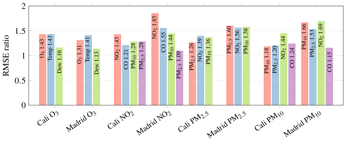
To add some insight on interpretability, a feature importance analysis is included. For each trained model we computed permutation importance by randomly shuffling the values of a single input feature across the test set (without changing the time dimension) and measuring the resulting increase in RMSE. A larger RMSE growth indicates greater feature importance because perturbing that feature degrades predictive performance more strongly. Figure 7 reports the average RMSE increase per feature for each pollutant. Results show the expected pattern for ${\mathrm{NO}}_2$: The pollutant’s own past values are consistently the most important predictor. However, for ${\mathrm{PM}}_{10}$, permuting ${\mathrm{NO}}_2$ produces the largest RMSE increase, indicating a strong predictive link between ${\mathrm{NO}}_2$ and ${\mathrm{PM}}_{10}$ in our datasets. For ${\mathrm{O}}_3$, temperature is the most influential feature, while for ${\mathrm{PM}}_{2.5}$ the importance is more uniformly distributed across the considered inputs. We also observe city-specific differences: for example, CO is a key contributor to ${\mathrm{NO}}_2$ prediction in Madrid but is comparatively less important in Cali.

These feature-importance patterns are consistent with the physical and urban context of the studied areas, although they should be interpreted as learned statistical associations rather than direct causal attribution. For ${\mathrm{O}}_3$, the dominant role of temperature is coherent with the photochemical production of ozone, which is strongly modulated by solar radiation and thermal conditions. For ${\mathrm{NO}}_2$, the strong importance of the pollutant’s own recent history, together with the contribution of CO in Madrid, is compatible with the influence of combustion-related urban traffic emissions, which are a major local source in both cities and particularly relevant in Madrid. In the case of ${\mathrm{PM}}_{10}$, the high relevance of ${\mathrm{NO}}_2$ suggests that the model is exploiting traffic-related co-variation, likely linked to both exhaust emissions and mechanically resuspended road dust. This interpretation is also consistent with the known source context of Madrid, where traffic dominates and episodic Saharan dust intrusions can further increase particulate concentrations, and of Cali, where particulate matter is influenced not only by mobile sources but also by seasonal regional biomass burning. The more uniform importance distribution observed for ${\mathrm{PM}}_{2.5}$ is also reasonable, as fine particulate matter often reflects the combined effect of several correlated variables rather than a single dominant predictor.

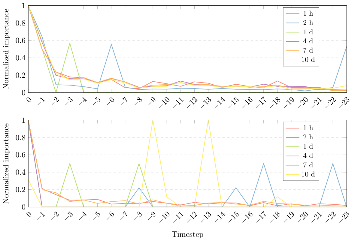
To examine the temporal contribution of past observations, we applied a SHAP analysis (Lundberg and Lee [42]). SHAP is an interpretability method based on cooperative game theory that quantifies the contribution of each input feature to a given prediction. In our case, it was used to estimate the relative importance of past timesteps by measuring how much each temporal input contributes to the model output. We used the ${\mathrm{PM}}_{10}$ model (single seed) as a representative example. The SHAP analysis used a background set of 100 samples and explained predictions for a random subset of 150 test samples; the model was re-evaluated 25 times to stabilize estimates. We averaged the absolute SHAP values per time-lag to obtain a single importance score for each past timestep. Figure 8 presents these timestep-averaged SHAP values across forecast horizons normalized to the range $[0,1]$. In both cities the most recent timestep is generally the most important predictor, but temporal importance is more evenly distributed in Cali. In Madrid (which has a shorter dataset), some long-horizon models (1-, 4-, and 7-day forecasts) rely on a narrower set of recent timesteps, suggesting a reduced capacity to capture long-term temporal structure. These temporal relevance patterns suggest that the models rely on different balances of short-term persistence and distributed temporal context depending on the city and forecast horizon, which is plausible given the differences in data availability, source mixture, and atmospheric variability between Madrid and Cali. Alternatively, averaging the SHAP values across features reveals that PM10 is the most influential predictor in Cali, whereas PM2.5 and distance contribute the least. In Madrid, PM10 and CO emerge as the most important predictors, while distance remains the least relevant feature. This indicates that temporal dynamics play a more significant role in PM10 forecasting than spatial relationships. However, distance is the dominant feature for the 1-day forecasting horizon, likely because temporal variability is partially constrained by periodic behavior at short lead times, but its importance progressively declines for longer forecasting horizons.

Regarding the training speed, the average training time for each of the selected models is included in

Table 10. Training time for the selected models in minutes.

Time	Cali				Madrid
Lag	${\mathbf{O}}_{\mathbf{3}}$	${\mathbf{NO}}_{\mathbf{2}}$	${\mathbf{PM}}_{\mathbf{2.5}}$	${\mathbf{PM}}_{\mathbf{10}}$	${\mathbf{O}}_{\mathbf{3}}$	${\mathbf{NO}}_{\mathbf{2}}$	${\mathbf{PM}}_{\mathbf{2.5}}$	${\mathbf{PM}}_{\mathbf{10}}$
1 h	47.6	40.2	35.7	18.0	5.6	4.9	11.5	7.4
2 h	16.8	40.2	32.3	42.3	2.9	7.6	7.0	8.4
1 d	46.1	36.8	27.1	41.5	2.5	7.1	12.0	9.9
4 d	34.4	32.9	75.3	39.0	3.4	13.4	8.6	9.9
7 d	9.9	38.0	37.9	40.2	6.5	10.8	11.2	15.0
10 d	9.1	30.5	44.6	21.9	4.0	5.2	10.9	3.2

. The number of samples used for Cali is, approximately, three times higher. However, the training takes 5.4 times longer, on average. All the experiments were conducted on a system equipped with 144 Intel^® Xeon^® Gold 5220 CPUs except for the ozone models, which additionally used a NVIDIA^® Tesla^® M10.

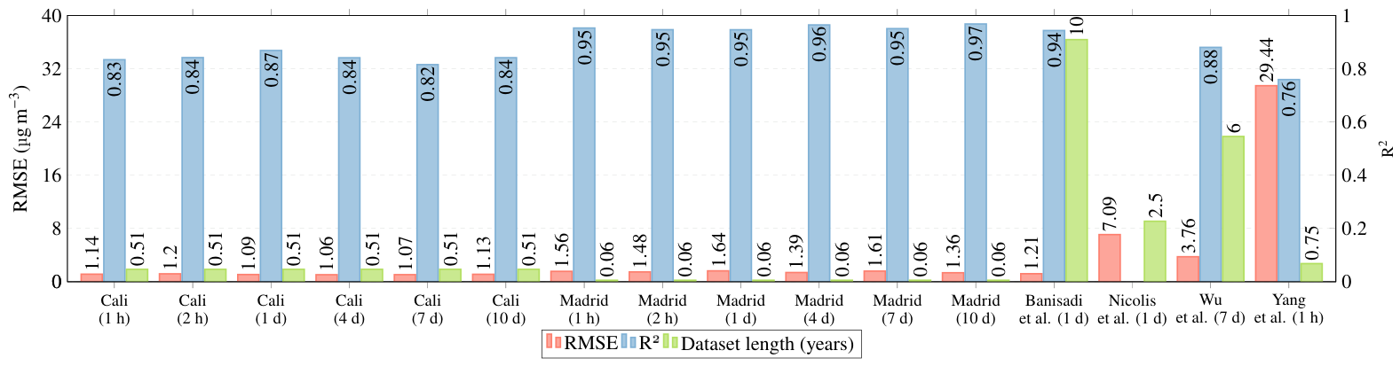
To offer a meaningful comparison between our model and the work of other authors, we have selected ${\mathrm{PM}}_{2.5}$, the most widely studied pollutant in the literature. Coincidentally, it was the pollutant that gave the worst performance in the validation set in terms of ${\mathrm{R}}^2$, as evidenced by Table A8. Figure 9 presents a comparative overview of our results against those reported in other studies from Section 1.1, which also address simultaneous spatial prediction and temporal forecasting for ${\mathrm{PM}}_{2.5}$. The comparison includes published results from Baniasadi et al. [7], Yang et al. [26] (averaging all the stations listed in Table 2 of their study), Nicolis et al. [16] (who did not report ${\mathrm{R}}^2$ for temporal forecasting), and Wu et al. [25] (for whom we selected the best-performing time lag, 7 days, among their four proposed horizons). It is important to note that these results were obtained under different conditions—each study used its own dataset, city, model, and forecasting horizon—which should be considered when interpreting the comparison. Furthermore, since most studies assess model performance at sensor locations seen during training, we used our validation set results to ensure a more equitable comparison framework.

Among the reviewed studies, Baniasadi et al. [7] demonstrated comparable performance by employing an LSTM model that was optimized with a binary chimp optimization algorithm. However, it should be noted that the model was trained using a dataset that spanned a decade, a significantly more extensive dataset than the one used in this study. The required effort and computation cost of training a model with such a large dataset may not justify the marginal gains, especially when our models achieved similar results with far fewer data. Additionally, urban environments evolve continuously, and data from a decade ago may no longer reflect current conditions. Thus, excessively long datasets may even hinder model performance by introducing outdated patterns that are no longer representative of the present-day cityscape.

For most pollutants and time lags, the best-performing model for Madrid tended to achieve higher ${\mathrm{R}}^2$ scores than the best-performing model for Cali. However, it should be noted that pollutants may have a seasonal variance, and some studies (Fioravanti et al. [18]) have even developed separate models for each month. To analyze these results, we tested the same models against the data from the last two weeks of December. Results are shown in

Table 11. RMSE for the selected models in the last two weeks of December 2024. No valid sample could be created for ${\mathrm{O}}_3$ in Madrid.

Time	Cali				Madrid
Lag	${\mathbf{O}}_{\mathbf{3}}$	${\mathbf{NO}}_{\mathbf{2}}$	${\mathbf{PM}}_{\mathbf{2.5}}$	${\mathbf{PM}}_{\mathbf{10}}$	${\mathbf{O}}_{\mathbf{3}}$	${\mathbf{NO}}_{\mathbf{2}}$	${\mathbf{PM}}_{\mathbf{2.5}}$	${\mathbf{PM}}_{\mathbf{10}}$
1 h	2.7803	2.2424	3.3025	5.1006	NaN	8.8976	4.9439	6.5915
2 h	4.2251	2.3084	3.2287	6.2525	NaN	8.9604	5.3485	8.9340
1 d	2.8997	2.4375	4.1200	7.4796	NaN	8.9016	6.1436	10.7410
4 d	4.5900	2.2095	3.8569	7.1081	NaN	18.3493	8.4711	13.3789
7 d	6.1595	2.4680	3.7579	5.4434	NaN	8.3916	6.4402	11.8535
10 d	6.0881	2.2847	3.9578	5.6520	NaN	8.9464	11.0111	9.1025

, and additional metrics are provided in

Table A16. MAE for the selected models in the last two weeks of December 2024.

Time	Cali				Madrid
Lag	${\mathbf{O}}_{\mathbf{3}}$	${\mathbf{NO}}_{\mathbf{2}}$	${\mathbf{PM}}_{\mathbf{2.5}}$	${\mathbf{PM}}_{\mathbf{10}}$	${\mathbf{NO}}_{\mathbf{2}}$	${\mathbf{PM}}_{\mathbf{2.5}}$	${\mathbf{PM}}_{\mathbf{10}}$
1 h	2.1939	1.7343	2.6213	3.9246	7.9818	3.6954	5.1971
2 h	3.3934	1.7707	2.5823	4.6682	7.7828	4.0227	6.7785
1 d	2.3754	1.8823	3.3690	5.6831	7.3737	4.8715	8.6431
4 d	3.8323	1.6815	3.1039	5.2425	16.5653	6.9792	10.5154
7 d	5.5442	1.9202	3.1061	4.3022	6.2674	4.6197	9.6491
10 d	5.3381	1.7602	3.1721	4.5663	7.6084	9.4953	7.3503

,

Table A17. SMAPE for the selected models in the last two weeks of December 2024.

Time	Cali				Madrid
Lag	${\mathbf{O}}_{\mathbf{3}}$	${\mathbf{NO}}_{\mathbf{2}}$	${\mathbf{PM}}_{\mathbf{2.5}}$	${\mathbf{PM}}_{\mathbf{10}}$	${\mathbf{NO}}_{\mathbf{2}}$	${\mathbf{PM}}_{\mathbf{2.5}}$	${\mathbf{PM}}_{\mathbf{10}}$
1 h	25.093	15.024	20.818	13.649	52.802	40.464	29.331
2 h	31.813	15.282	19.319	16.439	51.079	43.772	35.454
1 d	24.091	16.005	24.510	20.235	46.807	49.981	40.993
4 d	33.965	14.551	22.573	16.838	83.236	74.289	64.776
7 d	45.531	16.407	22.682	14.604	39.621	55.584	49.253
10 d	43.061	15.434	23.843	16.454	48.310	70.267	28.397

and

Table A18. MBE for the selected models in the last two weeks of December 2024.

Time	Cali				Madrid
Lag	${\mathbf{O}}_{\mathbf{3}}$	${\mathbf{NO}}_{\mathbf{2}}$	${\mathbf{PM}}_{\mathbf{2.5}}$	${\mathbf{PM}}_{\mathbf{10}}$	${\mathbf{NO}}_{\mathbf{2}}$	${\mathbf{PM}}_{\mathbf{2.5}}$	${\mathbf{PM}}_{\mathbf{10}}$
1 h	−0.8154	0.4698	0.4038	1.7471	−7.5200	−1.8265	−0.0736
2 h	−2.6360	0.5482	−0.2723	2.0634	−7.1491	−2.0166	−2.2089
1 d	−1.4205	0.7338	−0.9037	2.4232	−5.7650	−1.5790	−1.3816
4 d	−3.6370	0.5386	−1.6881	−0.9108	−16.3452	−2.4987	4.9172
7 d	−5.3504	0.3000	−2.4844	−1.1287	−1.6669	4.0318	5.6632
10 d	−5.0535	1.0038	−2.8426	−2.0087	−5.2263	−6.5994	−4.4635

. Specifically, the RMSE increased an average of 25.8% for the Cali predictions and 52.4% for the Madrid predictions. This loss of precision is especially significant for ${\mathrm{NO}}_2$ and for longer-term forecasting. Given the limited number of results, we have opted not to include the ${\mathrm{R}}^2$ metric, as it tends to be misleading for a small number of samples.

While these results may initially appear to support the approach of model separation by time intervals, performance significantly degrades when we are out of the training time range by up to two weeks. Although the levels of pollutants exhibit seasonal patterns, they are not periodic and vary from year to year. By separating the model by months, we not only reduce the size of the training dataset by twelve, but we also intentionally introduce overfitting into our model, which degrades its ability to generalize. Therefore, the model’s ability to make predictions for unseen pollution levels is diminished.

To analyze the temporal stability of the proposed deep learning framework, we retrained the selected models using an extended dataset, which is also publicly available in Alvarado-Alcon et al. [33]. This dataset spans from the initial dates reported in Table 3 up to 25 April 2026, thus covering more than one full year for both cities. We preserved the same preprocessing pipeline and station partitioning used in the previous experiments, ensuring that evaluation remains based on held-out monitoring stations. For this extended setting, samples up to 10 September 2026 were used for training and validation, while the final 7.5 months were reserved for testing, thereby enabling evaluation on both unseen locations and unseen future time periods. The results, summarized in

Table 12. RMSE obtained with the selected models trained on the extended dataset and evaluated on held-out monitoring stations using a later time period.

Time	Cali				Madrid
Lag	${\mathbf{O}}_{\mathbf{3}}$	${\mathbf{NO}}_{\mathbf{2}}$	${\mathbf{PM}}_{\mathbf{2.5}}$	${\mathbf{PM}}_{\mathbf{10}}$	${\mathbf{O}}_{\mathbf{3}}$	${\mathbf{NO}}_{\mathbf{2}}$	${\mathbf{PM}}_{\mathbf{2.5}}$	${\mathbf{PM}}_{\mathbf{10}}$
1 h	1.9912	2.9925	3.0479	6.8903	3.6432	8.5439	2.1452	6.9880
2 h	3.4720	1.2644	3.3038	8.1849	4.1519	7.4627	2.5579	8.2239
1 d	6.1346	5.3338	4.7682	13.3902	4.7176	6.0144	3.7396	7.9866
4 d	7.7901	5.2310	6.1140	5.5809	8.1360	4.9722	5.1688	14.0851
7 d	13.6714	5.7653	7.0925	5.9343	4.0410	7.3846	4.2379	13.9576
10 d	15.5405	5.0809	6.4908	7.5667	10.9007	15.9850	5.5934	10.7095

, show that the proposed framework remains effective when trained on longer and more diverse datasets. In many cases, particularly for shorter forecasting horizons, the models achieve lower RMSE values than in the original experiments, indicating improved stability and learning from the increased data volume. However, a degradation in performance can still be observed for longer forecasting horizons (7 and 10 days), which remain inherently more challenging due to the increased uncertainty and weaker temporal correlations at extended lead times.

To assess operational robustness under missing data, we performed an additional experiment on the extended test subset in which non-distance input values from already constructed sliding windows were randomly replaced by the mean value of the corresponding feature and timestep (or by 0.5 when all values for a given feature and timestep were removed). The results show that the framework is highly resilient to randomly distributed missingness once a valid input window can be constructed. In Madrid, averaging across pollutants and forecast horizons, the RMSE increased by only about 0.6% for each additional 10% of substituted values between 0% and 70% missingness. In Cali, the same analysis showed no meaningful average change in RMSE over that range. Even in the most affected individual case, ${\mathrm{PM}}_{2.5}$ forecasting at a 7-day horizon in Madrid, the RMSE increase remained below 30% when 60% of the non-distance inputs were replaced. These results indicate that the trained framework is robust to substantial levels of random input corruption at inference time. Nevertheless, this experiment reflects an optimistic missing-data pattern, since real sensor outages are typically structured and continuous rather than randomly distributed. In operational deployments, missingness often arises from prolonged hardware or communication failures, which may remove the observations of multiple sensors for periods longer than the 24-h sliding window. Under these conditions, spatial information is effectively lost, and forcing predictions through aggressive imputation becomes considerably less reliable. This is consistent with the imputation technique analysis, in which more aggressive strategies led to RMSE increases of up to 74.3%, far exceeding the degradation observed under randomly distributed missingness at inference time. Therefore, while the present robustness analysis supports the operational resilience of the framework to random missing values, evaluating structured and prolonged outage scenarios remains an important limitation of air quality forecasting and a relevant direction for future work.

Finally, we note that the proposed approach is amenable to real-world, online deployment because inference is computationally lightweight. In our experiments the average inference time for the complete validation set was 2.5 s for the Cali models and 1.9 s for the Madrid models. The heatmaps shown in Figure 1 and Figure 2 were generated at moderate spatial resolutions (Cali: 40 × 80 grid points; Madrid: 50 × 50 grid points) and each was produced in under one minute using a single seed. These timings imply that citywide heatmaps can be recomputed on an hourly cadence without prohibitive compute cost, making the system suitable for near-real-time dashboards, public alerts, or integration with traffic and urban management tools.

5. Discussion

In this study, we developed and evaluated a deep learning methodology that integrates temporal forecasting and spatial predictions to estimate cross-location citywide air pollution levels up to 10 days in advance. Specifically, our model enables fine-grained city-scale pollutant forecasting by inferring concentrations even in areas without sensors, leveraging spatial correlations learned from monitored locations. In addition, a comprehensive and comparative analysis of the model and imputation technique selection for different cities, pollutants, and time horizons is provided.

Our results indicate that, in general, LSTM×2 performed best for 1-hour time lag, while GRU×2 and LSTMGRU were as effective for longer time lags. However, the optimal model varied depending on the pollutant, city, and prediction horizon. For example, there is no overall difference between these three models for Cali, whereas in Madrid, we see a dominance of the LSTM×2 model. Models with two recurrent layers consistently outperformed those with a single recurrent layer or CNN, highlighting the benefits of increased model complexity. Notably, even the most complex architectures, with up to 61,953 trainable parameters, achieved satisfactory performance using less than a month of training data and approximately a thousand samples, far surpassing traditional methods such as RF.

Our findings also reveal several key insights. First, data imputation generally degraded model performance, with simple traditional approaches like mean imputation proving unreliable. Instead, discarding missing values or employing more refined imputation techniques that alter fewer records yielded much better results. A proper selection of the model and imputation technique may reduce the RMSE by up to 115%. While larger datasets spanning several years can enhance model performance, we demonstrated that comparable results can be achieved with significantly smaller datasets. This reduces both computational cost and training effort. For applications where minor accuracy differences are acceptable, smaller datasets offer a practical and efficient alternative, simplifying model maintenance and updates.

A limitation of the present framework is that spatial transfer is conditioned primarily through inter-sensor distance and the selected historical variables, without explicitly encoding anisotropic transport processes such as wind direction, wind speed, terrain elevation, or urban-topology effects. Urban pollutant dispersion is often strongly directional and source-dependent, especially for particulate matter and traffic-related gases, and these phenomena cannot be fully captured by distance alone. Although meteorological variables such as temperature, humidity, and dew point are included when supported by feature selection, future extensions could benefit from incorporating additional meteorological and geographic descriptors to better represent directional transport and urban morphology.

As future work, we plan to improve the spatial and temporal modeling capabilities of the framework by exploring more expressive architectures, such as Graph Neural Networks and advanced recurrent models, as well as by incorporating additional contextual inputs including day-of-week, holiday indicators, and weather forecasts. We also aim to remove the dependence on a canonical station order by investigating richer representations of sensing locations, such as altitude, terrain type, and urban morphology, which could also support sensor-importance analyses to identify critical or redundant monitoring sites. From an evaluation and deployment perspective, future work should examine the framework under alternative validation strategies, such as spatially blocked validation, to better assess its suitability for geographical extrapolation beyond the monitored urban domain. In addition, although the present results demonstrate robustness to random missing values, further research is needed on more challenging operational scenarios involving structured or prolonged sensor outages, as well as on transfer learning techniques to facilitate the adaptation of trained models to new cities.

References

1. The United Nations Population Division. Urban Population (% of Total Population). 2018. Available online: https://data.worldbank.org/indicator/SP.URB.TOTL.IN.ZS (accessed on 3 September 2025).
2. The Economic Times. Delhi pollution: More areas in ‘severe’ category, fines of Rs 5.85 cr imposed as restrictions tightened. The Economic Times, 16 November 2024. Available online: https://economictimes.indiatimes.com/news/india/traffic-police-in-delhi-slaps-fines-totalling-rs-1-crore-for-violations-after-grap-3-invoked/articleshow/115363438.cms (accessed on 21 January 2025).
3. The Sun. India court tells smog-hit capital to step up vehicle restrictions. The Sun, 22 November 2024. Available online: https://thesun.my/world-news/india-court-tells-smog-hit-capital-to-step-up-vehicle-restrictions-GD13328680 (accessed on 21 January 2025).
4. Drewil, G.I.; Al-Bahadili, R.J. Air pollution prediction using LSTM deep learning and metaheuristics algorithms. Meas. Sens. 2022, 24, 100546. [Google Scholar] [CrossRef] [Scilit]
5. Bekkar, A.; Hssina, B.; Douzi, S.; Douzi, K. Air-pollution prediction in smart city, deep learning approach. J. Big Data 2021, 8, 161. [Google Scholar] [CrossRef] [Scilit] [PubMed]
6. Wan, Y.; Xu, M.; Huang, H.; Xi Chen, S. A spatio-temporal model for the analysis and prediction of fine particulate matter concentration in Beijing. Environmetrics 2021, 32, e2648. [Google Scholar] [CrossRef] [Scilit]
7. Baniasadi, S.; Salehi, R.; Soltani, S.; Martín, D.; Pourmand, P.; Ghafourian, E. Optimizing Long Short-Term Memory Network for Air Pollution Prediction Using a Novel Binary Chimp Optimization Algorithm. Electronics 2023, 12, 3985. [Google Scholar] [CrossRef] [Scilit]
8. Rabie, R.; Asghari, M.; Nosrati, H.; Emami Niri, M.; Karimi, S. Spatially resolved air quality index prediction in megacities with a CNN-Bi-LSTM hybrid framework. Sustain. Cities Soc. 2024, 109, 105537. [Google Scholar] [CrossRef] [Scilit]
9. Shiri, F.M.; Perumal, T.; Mustapha, N.; Mohamed, R. A comprehensive overview and comparative analysis on deep learning models: CNN, RNN, LSTM, GRU. arXiv 2023, arXiv:2305.17473. [Google Scholar] [CrossRef] [Scilit]
10. Zhang, Z.; Zhang, S.; Chen, C.; Yuan, J. A systematic survey of air quality prediction based on deep learning. Alex. Eng. J. 2024, 93, 128–141. [Google Scholar] [CrossRef] [Scilit]
11. Tao, Q.; Liu, F.; Li, Y.; Sidorov, D. Air Pollution Forecasting Using a Deep Learning Model Based on 1D Convnets and Bidirectional GRU. IEEE Access 2019, 7, 76690–76698. [Google Scholar] [CrossRef] [Scilit]
12. Bhatta, J.; Acharya, S.R.; Yang, K.M. Machine learning-enhanced air quality forecasting and trend analysis: A five-year comprehensive assessment of PM2.5 concentrations in Bangkok, Thailand. Environ. Chall. 2026, 22, 101442. [Google Scholar] [CrossRef] [Scilit]
13. Bougoudis, I.; Demertzis, K.; Iliadis, L. HISYCOL a hybrid computational intelligence system for combined machine learning: The case of air pollution modeling in Athens. Neural Comput. Appl. 2016, 27, 1191–1206. [Google Scholar] [CrossRef] [Scilit]
14. Apte, J.S.; Messier, K.P.; Gani, S.; Brauer, M.; Kirchstetter, T.W.; Lunden, M.M.; Marshall, J.D.; Portier, C.J.; Vermeulen, R.C.; Hamburg, S.P. High-Resolution Air Pollution Mapping with Google Street View Cars: Exploiting Big Data. Environ. Sci. Technol. 2017, 51, 6999–7008. [Google Scholar] [CrossRef] [Scilit] [PubMed]
15. Hu, X.; Belle, J.H.; Meng, X.; Wildani, A.; Waller, L.A.; Strickland, M.J.; Liu, Y. Estimating PM2.5 Concentrations in the Conterminous United States Using the Random Forest Approach. Environ. Sci. Technol. 2017, 51, 6936–6944. [Google Scholar] [CrossRef] [Scilit] [PubMed]
16. Nicolis, O.; Díaz, M.; Sahu, S.K.; Marín, J.C. Bayesian spatiotemporal modeling for estimating short-term exposure to air pollution in Santiago de Chile. Environmetrics 2019, 30, e2574. [Google Scholar] [CrossRef] [Scilit]
17. Kalajdjieski, J.; Zdravevski, E.; Corizzo, R.; Lameski, P.; Kalajdziski, S.; Pires, I.M.; Garcia, N.M.; Trajkovik, V. Air Pollution Prediction with Multi-Modal Data and Deep Neural Networks. Remote. Sens. 2020, 12, 4142. [Google Scholar] [CrossRef] [Scilit]
18. Fioravanti, G.; Martino, S.; Cameletti, M.; Cattani, G. Spatio-temporal modelling of PM10 daily concentrations in Italy using the SPDE approach. Atmos. Environ. 2021, 248, 118192. [Google Scholar] [CrossRef] [Scilit]
19. Shahriar, S.A.; Kayes, I.; Hasan, K.; Hasan, M.; Islam, R.; Awang, N.R.; Hamzah, Z.; Rak, A.E.; Salam, M.A. Potential of ARIMA-ANN, ARIMA-SVM, DT and CatBoost for Atmospheric PM2.5 Forecasting in Bangladesh. Atmosphere 2021, 12, 100. [Google Scholar] [CrossRef] [Scilit]
20. Kristiani, E.; Lin, H.; Lin, J.R.; Chuang, Y.H.; Huang, C.Y.; Yang, C.T. Short-Term Prediction of PM2.5 Using LSTM Deep Learning Methods. Sustainability 2022, 14, 2068. [Google Scholar] [CrossRef] [Scilit]
21. Saez, M.; Barceló, M.A. Spatial prediction of air pollution levels using a hierarchical Bayesian spatiotemporal model in Catalonia, Spain. Environ. Model. Softw. 2022, 151, 105369. [Google Scholar] [CrossRef] [Scilit]
22. Kumar, K.; Pande, B.P. Air pollution prediction with machine learning: A case study of Indian cities. Int. J. Environ. Sci. Technol. 2023, 20, 5333–5348. [Google Scholar] [CrossRef] [Scilit] [PubMed]
23. Samad, A.; Garuda, S.; Vogt, U.; Yang, B. Air pollution prediction using machine learning techniques – An approach to replace existing monitoring stations with virtual monitoring stations. Atmos. Environ. 2023, 310, 119987. [Google Scholar] [CrossRef] [Scilit]
24. Rahman, M.M.; Nayeem, M.E.H.; Ahmed, M.S.; Tanha, K.A.; Sakib, M.S.A.; Uddin, K.M.M.; Babu, H.M.H. AirNet: Predictive machine learning model for air quality forecasting using web interface. Environ. Syst. Res. 2024, 13, 44. [Google Scholar] [CrossRef] [Scilit]
25. Wu, Z.; Tian, Y.; Li, M.; Wang, B.; Quan, Y.; Liu, J. Prediction of air pollutant concentrations based on the long short-term memory neural network. J. Hazard. Mater. 2024, 465, 133099. [Google Scholar] [CrossRef] [Scilit] [PubMed]
26. Yang, W.; Wu, Q.; Li, J.; Chen, X.; Du, H.; Wang, Z.; Li, D.; Tang, X.; Sun, Y.; Ye, Z.; et al. Predictions of air quality and challenges for eliminating air pollution during the 2022 Olympic Winter Games. Atmos. Res. 2024, 300, 107225. [Google Scholar] [CrossRef] [Scilit]
27. Zareba, M.; Cogiel, S.; Danek, T.; Weglinska, E. Machine Learning Techniques for Spatio-Temporal Air Pollution Prediction to Drive Sustainable Urban Development in the Era of Energy and Data Transformation. Energies 2024, 17, 2738. [Google Scholar] [CrossRef] [Scilit]
28. Illescas-Martinez, F.; Garcia, L.; Garcia-Sanchez, A.J.; Asorey-Cacheda, R.; Garcia-Haro, J. Air quality forecasting in non-monitored urban areas through machine and deep-learning model. Expert Syst. Appl. 2025, 284, 127749. [Google Scholar] [CrossRef] [Scilit]
29. Xia, H.; Chen, X.; Chen, B.; Hu, Y. Dynamic synchronous graph transformer network for region-level air-quality forecasting. Neurocomputing 2025, 616, 128924. [Google Scholar] [CrossRef] [Scilit]
30. Zhang, C.; Niu, X.; Wu, H.; Ding, Z.; Chan, K.L.; Kim, J.; Wagner, T.; Liu, C. Unleashing the potential of geostationary satellite observations in air quality forecasting through artificial intelligence techniques. Atmos. Chem. Phys. 2025, 25, 759–770. [Google Scholar] [CrossRef] [Scilit]
31. Panja, M.; Chakraborty, T.; Biswas, A.; Deb, S. E-STGCN: Extreme spatio-temporal graph convolutional networks for air quality forecasting. J. R. Stat. Soc. Ser. A Stat. Soc. 2026, qnag010. [Google Scholar] [CrossRef] [Scilit]
32. Santiago, J.L.; Martín, F.; Martilli, A. A computational fluid dynamic modelling approach to assess the representativeness of urban monitoring stations. Sci. Total. Environ. 2013, 454–455, 61–72. [Google Scholar] [CrossRef] [Scilit] [PubMed]
33. Alvarado-Alcon, F.J.; Asorey-Cacheda, R.; Garcia-Haro, J.; García, L.; Garcia-Sanchez, A.J. Replication Data for “Citywide Air Quality Forecasting over Sparse Sensor Networks: Cross-Location Generalization and Deep Learning Reliability under Missing Data”; Zenodo: Geneva, Switzerland, 2026. [Google Scholar] [CrossRef]
34. Glorot, X.; Bengio, Y. Understanding the difficulty of training deep feedforward neural networks. In Proceedings of the Thirteenth International Conference on Artificial Intelligence and Statistics Proceedings of Machine Learning Research, Sardinia, Italy, 13–15 May 2010; Proceedings of Machine Learning Research; Teh, Y.W., Titterington, M., Eds.; Journal of Machine Learning Research: Brookline, MA, USA, 2010; Volume 9, pp. 249–256. [Google Scholar]
35. Alvarado-Alcon, F.J.; Asorey-Cacheda, R.; Garcia-Sanchez, A.J.; Garcia-Haro, J.; García, L. Loss-Versus-Epoch Graphs for “Deep Learning for Citywide Air Quality Inference: Cross-location Forecasting from Sparse Stations”; Zenodo: Geneva, Switzerland, 2025. [Google Scholar] [CrossRef]
36. AQI India API. AQI India API. 2010. Available online: https://www.kaggle.com/datasets/omsandeeppatil/indian-aqi-stations (accessed on 31 December 2024).
37. Hastie, T.; Tibshirani, R.; Friedman, J. The Elements of Statistical Learning: Data Mining, Inference, and Prediction, 2nd ed.; Springer: Berlin/Heidelberg, Germany, 2009; Chapter 7. [Google Scholar]
38. Alazmi, A.; Rakha, H. Assessing and validating the ability of machine learning to handle unrefined particle air pollution mobile monitoring data randomly, spatially, and spatiotemporally. Int. J. Environ. Res. Public Health 2022, 19, 10098. [Google Scholar] [CrossRef] [Scilit] [PubMed]
39. Dirección General de Sostenibilidad y Control Ambiental. Calidad del Aire 2023. 2023. Available online: https://airedemadrid.madrid.es/UnidadesDescentralizadas/Sostenibilidad/CalidadAire/Publicaciones/Memorias_anuales/Ficheros/MEMORIA_2023_01.pdf (accessed on 4 September 2025).
40. Mateus-Fontecha, L.; Vargas-Burbano, A.; Jimenez, R.; Rojas, N.Y.; Rueda-Saa, G.; van Pinxteren, D.; van Pinxteren, M.; Fomba, K.W.; Herrmann, H. Understanding aerosol composition in a tropical inter-Andean valley impacted by agro-industrial and urban emissions. Atmos. Chem. Phys. 2022, 22, 8473–8495. [Google Scholar] [CrossRef] [Scilit]
41. OpenStreetMap Contributors. Open Street Map. 2015. Available online: https://www.openstreetmap.org (accessed on 11 February 2026).
42. Lundberg, S.M.; Lee, S.I. A unified approach to interpreting model predictions. In Proceedings of the 31st International Conference on Neural Information Processing Systems, Red Hook, NY, USA, 4–9 December 2017; pp. 4768–4777. [Google Scholar]
Figure 3. Number of valid records per city after applying different missing data handling approaches. The expected number of records under ideal conditions, without missing data, is 7920 for Madrid and 89,760 for Cali.
Jsan 15 00052 g003
Figure 4. Number of samples per city after applying different missing data handling approaches. For each city, six datasets are presented, corresponding to predictions for 1 h, 2 h, 1 d, 4 d, 7 d, and 10 d time horizons. The expected number of samples under ideal conditions for 1-hour forecasting, without missing data, is 1584 for Madrid and 8976 for Cali.
Jsan 15 00052 g004
Figure 5. RMSE obtained on sensors not used during training or validation, reported for each city, pollutant, and forecast horizon.
Jsan 15 00052 g005
Figure 6. R 2 obtained on sensors not used during training or validation, reported for each city, pollutant, and forecast horizon.
Jsan 15 00052 g006
Figure 7. Permutation feature importance as the average increase in RMSE when each input feature is randomly permuted across the test set. The first (red) bar for each pollutant corresponds to the pollutant’s own past values.
Jsan 15 00052 g007
Figure 8. Timestep importance for PM 10 for Cali (top) and Madrid (bottom) as the absolute SHAP values averaged per input timestep, shown for multiple forecast horizons. Larger values indicate greater contribution of that timestep to the model’s prediction.
Jsan 15 00052 g008
Figure 9. RMSE and R 2 for PM 2.5 inference in studies [7,16,25,26] that integrate temporal forecasting with spatial interpolation. The temporal horizon of each study is indicated in parentheses.
Jsan 15 00052 g009