Article

Mental Disorder Assessment in IoT-Enabled WBAN Systems with Dimensionality Reduction and Deep Learning

by
Damilola Olatinwo
1,†,
Adnan Abu-Mahfouz
1,2,*,† and
Hermanus Myburgh
1,†
1
Department of Electrical, Electronic and Computer Engineering, University of Pretoria, Pretoria 0002, South Africa
2
Council for Scientific and Industrial Research (CSIR), Pretoria 0184, South Africa
*
Author to whom correspondence should be addressed.
These authors contributed equally to this work.
J. Sens. Actuator Netw. 2025, 14(3), 49; https://doi.org/10.3390/jsan14030049
Submission received: 11 March 2025 / Revised: 29 April 2025 / Accepted: 30 April 2025 / Published: 7 May 2025

Abstract

:
Mental health is an important aspect of an individual’s overall well-being. Positive mental health is correlated with enhanced cognitive function, emotional regulation, and motivation, which, in turn, foster increased productivity and personal growth. Accurate and interpretable predictions of mental disorders are crucial for effective intervention. This study develops a hybrid deep learning model, integrating CNN and BiLSTM applied to EEG data, to address this need. To conduct a comprehensive analysis of mental disorders, we propose a two-tiered classification strategy. The first tier classifies the main disorder categories, while the second tier classifies the specific disorders within each main disorder category to provide detailed insights into classifying mental disorder. The methodology incorporates techniques to handle missing data (kNN imputation), class imbalance (SMOTE), and high dimensionality (PCA). To enhance clinical trust and understanding, the model’s predictions are explained using local interpretable model-agnostic explanations (LIME). Baseline methods and the proposed CNN–BiLSTM model were implemented and evaluated at both classification tiers using PSD and FC features. On unseen test data, our proposed model demonstrated a 3–9% improvement in prediction accuracy for main disorders and a 4–6% improvement for specific disorders, compared to existing methods. This approach offers the potential for more reliable and explainable diagnostic tools for mental disorder prediction.

1. Introduction

Mental disorders, such as schizophrenia, major depressive disorder, anxiety, and bipolar disorder, pose significant challenges to patients’ quality of life and overall well-being and contribute to high morbidity, mortality, and suicide rates. While presenting with distinct clinical features—for instance, schizophrenia characterized by delusions and hallucinations [1], major depressive disorder by emotional distress and increased suicide risk [2,3,4], anxiety by a combination of emotional, physical, and behavioral symptoms [5,6], and bipolar disorder by alternating episodes of mania and depression [7]—early detection and intervention remain critical for effective treatment and prevention [8]. Traditional diagnostic methods that rely on subjective self-reporting and clinical interviews, exemplified by depression diagnosis using patient interrogation and scales like the Hamilton Depression Rating Scale (HDRS) [9], are susceptible to patient biases and interpretation, thereby impacting diagnostic accuracy. This inherent subjectivity can also influence clinicians’ assessments, potentially leading to inaccuracies, particularly among less experienced practitioners. In response to these limitations, the integration of Internet of Things (IoT)-enabled wireless body area networks (WBANs) with artificial intelligence (AI) techniques (such as machine learning (ML) and deep learning (DL)) has emerged as a promising avenue for objective and continuous mental health monitoring.
IoT-enabled WBANs integrated with AI offer a powerful platform for acquiring the objective and continuous data necessary to fuel these advanced AI models. Typically, these WBANs consist of smart, lightweight wearable sensors (e.g., electroencephalogram (EEG) sensors, accelerometers, heart rate sensors, electrodermal activity sensors, and microphones) [10,11,12,13] that collect real-time physiological signals (e.g., brain activity, movement, heart rate variability, emotional arousal, and speech) to track mental health status and detect subtle changes indicative of underlying issues. Essentially, EEG captures and measures the electrical impulses of the brain, which can be used to study various aspects of brain activity, including different mental states, brain disorders, and neurological conditions [14]. Other sensors that can be used to collect data for the diagnosis and monitoring of mental disorders include accelerometers, which measure movement and physical activity levels, and heart rate sensors, which track heart rate variability, indicating stress and anxiety. Electrodermal activity sensors measure skin conductance, which can reflect emotional arousal and stress, and microphones record speech features that can indicate depressive symptoms. IoT-enabled WBANs with AI offer the potential to continuously track patients’ mental health status by analyzing these physiological signals to identify subtle changes indicative of underlying mental health issues.
Within the realm of AI-driven mental disorder prediction, a diverse range of approaches have been explored  [9,15,16,17,18,19,20,21,22,23,24]. Early efforts focused on traditional machine learning algorithms applied to features extracted from clinical interviews, questionnaires, and increasingly, physiological signals. For example, support vector machines (SVMs) and random forests have been employed to classify individuals with and without specific mental disorders based on features derived from speech patterns [25], textual analysis of patient narratives [26], and even basic physiological measures like heart rate variability [27,28]. More recently, the advent of DL has revolutionized the field, enabling the automatic extraction of complex patterns directly from raw data. Convolutional neural networks (CNNs) have shown promise in analyzing time-series data like electroencephalography (EEG) signals for identifying neural correlates of mental disorders [29,30]. Recurrent neural networks (RNNs), particularly long short-term memory (LSTM) networks and their bidirectional variants (BiLSTMs), have been effectively used to model temporal dependencies in sequential data, such as speech and electronic health records, for predicting the onset or progression of mental illness [31,32]. Furthermore, hybrid approaches that integrate the strengths of different DL architectures, such as CNNs for feature extraction and RNNs for sequence modeling, are increasingly recognized for their ability to harness complex data patterns effectively [33].
Accurate prediction of mental disorders is crucial for early detection and intervention. However, existing AI methods face several limitations that hinder their widespread clinical application. For instance, most classic ML models, particularly those relying on feature engineering from sources like questionnaires or clinical interviews, can suffer from the curse of dimensionality when dealing with a large number of potentially correlated or redundant features. This can lead to poor generalization to new, unseen data. While feature extraction (i.e., dimensionality reduction) techniques can mitigate this issue, their effectiveness depends on the specific dataset and clinical context. On the other hand, ML models, such as deep neural networks used for analyzing electronic health records, typically require very large, diverse, and well-annotated datasets to achieve robust performance and avoid biases. The limited availability of such datasets in mental health research can restrict the applicability and generalizability of these models. Furthermore, the decision-making processes of most developed models are not interpretable, which hinders their clinical adoption and trustworthiness. These limitations highlight the challenges in developing accurate and reliable models for predicting mental disorders.
To address these challenges, this study introduces a novel mental disorder predictor. Specifically, we propose a hybrid DL architecture based on a convolutional neural network (CNN) and bidirectional long short-term memory (BiLSTM) to learn the patterns and relationships within EEG signal data to predict mental health illnesses. The primary objectives of this study are twofold: to evaluate the effectiveness of feature extraction methods in mitigating the curse of dimensionality and improving prediction accuracy for mental disorders, and to introduce an explainability mechanism that enhances the interpretability of the model’s predictions. The findings of this study have significant implications for both mental health research and clinical practice. Demonstrating the efficacy of the proposed hybrid classifier in enhancing mental disorder prediction, we contribute to the advancement of this field. The key contributions of this study are outlined as follows:
  • We introduce a novel hybrid DL architecture based on a convolutional neural network (CNN) and bidirectional long short-term memory (BiLSTM) to learn the patterns and relationships within EEG signal data to predict mental health illnesses.
  • We address missing data using the k-nearest neighbors (kNN) data imputation method and the class imbalance issue using the synthetic minority over-sampling technique (SMOTE).
  • We employ principal component analysis (PCA) as a dimensionality reduction method to mitigate the curse of dimensionality and improve the prediction accuracy of the mental disorder model.
  • We employ the local interpretable model-agnostic explanations (LIME) method to interpret the predictions of the mental disorder model. This addresses the “black-box” problem often associated with the complex existing mental disorder models, making the results more understandable and trustworthy for clinicians and researchers.
The remainder of this paper is structured as follows. Section 2 presents a review of existing studies. Based on the insights from Section 2, Section 3 presents the methodology. Following this, Section 4 presents the results and discussion. Section 5 presents the limitation of the study, while Section 6 concludes the study by summarizing the key findings and highlighting their contributions.

2. Related Works

The diagnosis of mental health conditions typically involves a thorough psychiatric interview, an assessment of reported symptoms, a psychiatric history, and physical examinations [15]. In recent years, advancements in machine learning have garnered significant attention in predicting mental disorders. Researchers have proposed various machine learning (ML)-based mental disorder prediction models to support patients with mental health conditions and healthcare professionals across different settings.
For example, the authors of [16,17] developed mental health disorder prediction models for employees, aiming at early intervention and management to enhance their productivity. Yadav and Bokhari [16] investigated the performance of a hybrid classifier framework by combining decision trees (DT) with k-nearest neighbors (kNN) and random forest (RF) with neural networks (NNs). They used the mental health dataset from Kaggle, consisting of 27 features. The RF + NN model achieved an accuracy of 93.54%. Similarly, Jain et al. [17] proposed a DT-based mental health disorder prediction model for employees. Using the same Kaggle mental health dataset with 27 features, their proposed method outperformed other techniques like logistic regression (LR), RF, and kNN, achieving an accuracy of 82%. However, these studies [16,17] did not address the curse of dimensionality, and their models lacked interpretability in their decision-making processes, which is crucial for clinical acceptability.
The authors of [18,19] proposed mental health prediction models aimed at early psychological intervention for students in colleges and universities, with the goal of improving their academic performance. Shan [18] developed a graph neural network-based mental health disorder prediction model using mental health data with 20 features from Kaggle. They employed the implicit bulk surface filtering (IBSF) method to clean the data, achieving a 26.26% improvement in accuracy over other methods. Similarly, Sahu et al. [19] proposed a logistic regression-based mental health predictor model for university students. The experiment was conducted using data from questionnaires with 10 features. The proposed method was evaluated against other methods and achieved an accuracy of 61.90%. However, these studies did not consider feature extraction methods to address the curse of dimensionality, and the models lacked interpretability in their decision-making processes.
Moreover, some works have proposed predicting mental disorders in patients using questionnaires and physiological data. For instance, refs. [20,21] used clinical interviews and questionnaires. In this context, Niu et al. [20] proposed a hierarchical context-aware graph attention model (HCAG) for depression detection. They employed the Wizard of Oz (DAIC-WOZ) dataset for their experiment. The proposed model leverages hierarchical structures and graph attention mechanisms to capture contextual information from text, audio, and physiological signals, reporting an accuracy of 92%. Srividya1 et al. [21] investigated different machine learning methods such as LR, Naïve Bayes (NB), support vector machine (SVM), DT, kNN, bagging, and RF to predict patients’ mental states. They used questionnaires from two target populations with 20 features. Based on their investigation, the bagging and RF methods outperformed the other methods, with an accuracy of 90%.
The authors of [22,23,24,33] used physiological data to predict mental disorders. For example, Hassantabar et al. [22] proposed a deep neural network (DNN) to predict three mental disorders: schizoaffective, major depressive, and bipolar. They used physiological data from the Hackensack Meridian Health Carrier Clinic for the experiment. The performance of the proposed method was evaluated along with other ML methods, including SVM, DT, RF, kNN, NB, and AdaBoost. The DNN method achieved an accuracy of 90.4%. Wang et al. [23] proposed a bagging ensemble learning approach to predict depression using physiological data from different databases such as DAIC-WOZ, Kaggle, Reddit, and so on. Their proposed method achieved an accuracy of 87.32% when evaluated against other methods, including SVM, LR, kNN, DT, and case-based reasoning (CBR). Yadav et al. [24] proposed a convolutional neural network (CNN) method to predict depression. They used the depression dataset from Kaggle for their experiment. The proposed CNN method was evaluated using different machine learning methods, including logistic regression (LR), k-nearest neighbors (kNN), decision trees (DT), and bagging, achieving an accuracy of 93%.
Ahmed et al. [33] employed machine learning (ML) and deep learning (DL) methods, including k-nearest neighbors (kNN), artificial neural networks (ANNs), convolutional neural network–long short-term memory (CNN–LSTM), and bidirectional long short-term memory (BiLSTM), to predict mental disorders in patients using quantitative electroencephalography (EEG) data from Kaggle. The dataset comprised various main disorder categories, including addictive disorders, anxiety disorders, mood disorders, obsessive–compulsive disorders, schizophrenia, trauma-related disorders, alcohol disorders, and stress-related disorders, along with their specific disorders, including acute stress disorder, depression, behavioral addiction disorder, panic disorder, social anxiety disorder, post-traumatic stress disorder, adjustment disorder, and bipolar disorder. The dataset contained 1140 features. Using the entire dataset, ANN, CNN–LSTM, and BiLSTM achieved accuracies of 96.83% in predicting the main disorder categories, while kNN and LSTM achieved accuracies of 98.94% in predicting specific disorders. However, these existing studies [22,23,24,33] often lack effective feature extraction methods to mitigate the curse of dimensionality, which can lead to poor generalization performance. Furthermore, they lack interpretability mechanisms to explain the decision-making processes of their models, potentially limiting their clinical acceptance.

3. System Model

This section presents the development of a hybrid DL classifier (CNN–BiLSTM) for predicting mental disorders. The aim of this study is to classify patients’ mental disorders into major and specific categories. Our approach involves data collection, data cleaning and preprocessing, model development, model evaluation, results interpretation, model prediction explainability, and model prediction interpretability, as shown in Figure 1.

3.1. Mental Disorder Classification Task

The mental disorder dataset consists of a total number of instances denoted by D = { d 1 , d 2 , , d M } . The instances of the dataset are divided into two groups of attributes (features): main disorders and specific disorders. Each instance’s features of the main disorders and the specific disorders are represented by X = { x 1 , x 2 , x 3 , , x X } and X = { x 1 , x 2 , x 3 , , x X } , respectively. The main disorder-dependent class label is denoted as y n with a label space ( y n { 0 , 1 , 2 , 3 , 4 , 5 } ) that comprises six main classes of mental disorders: addictive disorders, anxiety disorders, mood disorders, obsessive–compulsive disorders, schizophrenia, and trauma- and stress-related disorders. The specific disorder-dependent class label is represented by y n with a label space ( y n { 0 , 1 , 2 , 3 , 4 , 5 , 6 , 7 , 8 } ) that comprises nine main classes of specific mental disorders: acute stress disorder, adjustment disorder, alcohol use disorder, behavioral addiction disorder, bipolar disorder, depressive disorder, panic disorder, post-traumatic stress disorder, and social anxiety disorder.
The objective of this study is to create a multiclass classification model using a hybrid DL method. For the main disorders, the model outputs the probabilities that indicate the likelihood of an instance belonging to each of the main disorder classes. Specifically, for each instance, the model provides a probability distribution over the six main mental disorder classes. The class with the highest probability is selected as the predicted main disorder class for that instance. For the specific disorders within each main class, the model outputs probabilities indicating the likelihood of an instance belonging to each of the nine specific mental disorder classes. Again, the class with the highest probability is selected as the predicted specific disorder class for that instance.
To achieve this, the proposed hybrid model first classifies the main mental disorders to provide a broad-spectrum analysis that identifies the general categories of mental health issues. Next, the model classifies the specific mental disorders within the broader main categories to offer detailed insight into the nuances of each disorder. The purpose of this study is to ensure that prompt interventions are more precisely tailored to individual patients’ needs. Identifying specific disorders at an early stage can help prevent their progression.

3.2. Mental Disorder Data Description

The dataset used in this study was sourced from a public repository [34,35] and consists of the medical records, psychological assessments, and EEG signals collected from patients with mental disorders and healthy controls using a Neuroscan device (EEG biomedical device) during a 5-min resting state. The collection spanned from January 2011 to December 2018 at SMG-SNU Boramae Medical Center, Seoul, South Korea. The dataset comprises patients aged 18–70, categorized into six main mental disorder groups: mood disorders, schizophrenia, addictive disorders, anxiety disorders, obsessive–compulsive disorders, and trauma- and stress-related disorders.
These main disorders were further categorized. For example, addictive disorders included behavioral addiction and alcohol use disorder; mood disorders encompassed bipolar disorder and depression; trauma- and stress-related disorders included post-traumatic stress disorder, acute stress disorder, and adjustment disorder; and anxiety disorders comprised social anxiety disorder and panic disorder. The dataset also included attributes such as age, IQ, sex, education, EEG recording date, and EEG frequencies (0.5–50 Hz) from 19 channels (FP1, FP2, F7, F3, Fz, F4, F8, T7, C3, Cz, C4, T8, P7, P3, Pz, P4, P8, O1, and O2).
The ground channel was placed between the Fz and FPz electrodes. EEG data were downsampled to 128 Hz, maintaining electrode impedances below five kilo-ohms. Using the Neuroguide system, the EEG data were converted to the frequency domain via a Fast Fourier Transform (FFT) with the following parameters: 0.5–40 Hz frequency range, 128 samples/sec, 2 sec epochs, and a 0.5 Hz resolution. The EEG parameters included the power spectral density (PSD) and functional connectivity (FC). These were computed into six frequency bands: delta, theta, alpha, beta, high-beta (25–30 Hz), and gamma. The dataset contained a total of 1140 features calculated as (19 PSD channels + 171 FC channels) × six bands [32].
The data excluded patients with certain medical histories: neurological disorders, brain injuries, neurodevelopmental disorders (IQ < 70 or borderline IQ of 70–80, attention deficit hyperactivity disorder), and neurocognitive disorders to ensure that the observed patterns in the data were more directly related to the mental disorder under investigation, rather than being potentially confounded by the effects of the other neurological or developmental conditions. These conditions can independently influence brain structure, function, and behavior, which could introduce variability and make it difficult to isolate the specific neural correlates or behavioral patterns associated with the mental disorder of interest [35]. EEG signals provide a non-invasive way to measure brain activity, making them valuable for studying mental disorders by capturing real-time electrical changes. For example, abnormal EEG patterns are associated with anxiety, schizophrenia, and mood disorders. Analyzing EEG data offers insights into the neural mechanisms of mental disorders, leading to improved diagnosis and treatment. Table 1 and Table 2 present the demographic descriptive statistics of the main and specific disorders, where n represents the sample size (i.e., the total number of participants in each class).

3.3. Data Cleaning and Preprocessing

The quality and integrity of the data directly impact the performance and reliability of a model. Thus, data cleaning and preprocessing are critical steps in the DL pipeline to develop a robust model for predicting mental illness. This section delves into the systematic methodologies employed to rectify data inconsistencies; including handling missing values, class imbalance, and transforming raw data into a format suitable for model training [36].

3.3.1. Addressing Missing Data Using the kNN Imputation Method

Handling missing data is vital for building robust DL models. The IQ and education attributes in the mental disorder data contain missing values, which can introduce bias and reduce statistical power. Figure 2 illustrates the intensity of the missing data, aiding in identifying patterns and determining the focus for data imputation. It highlights the missing values in the dataset using blue vertical lines, indicating gaps where data are missing. This visualization helps identify problematic areas that require correction before analysis. In this study, we used the kNN imputation method with sklearn.impute.KNNImputer to address the missing data. For each variable, the kNN imputation identified the k-nearest neighbors of an incomplete instance using the Minkowski distance [37] and then filled missing data with a weighted average of the neighbors. For example, suppose that x m represents an incomplete instance (row m) with a missing value, and x j m represents the j-th nearest neighbor of x m . The imputed value for the missing value in x m was computed using Equation (1):
x ^ m = j = 1 k w j x j m j = 1 k w j
where k denotes the number of nearest neighbors used to estimate the missing value x m , w j = 1 d ( x m , x j m ) , and d ( x m , x j m ) is the Minkowski distance computed using Equation (2):
d ( x m , x j m ) = p = 1 n | x p m x j , p m | q 1 q
where n is the number of dimensions, and x p m and x j , p m represent the p-th components of instances x m and x j m , respectively. The Minkowski coefficient q is set to 2, which represents the Euclidean distance. Given the relatively small number of missing values in the education (8 out of n samples) and IQ (11 out of n samples) features, we opted to use a common rule of thumb for selecting the number of neighbors (k) in the kNN imputer. A widely used heuristic suggests setting k to the square root of the number of samples in the dataset [38] or using a small fixed value such as 5 [39]. In our case, considering the modest amount of missing data, we chose a value of k = 5. This small value allows the imputation to be influenced by the most similar data points, potentially capturing local relationships without being overly smoothed by a large number of neighbors. Furthermore, with such a small fraction of missing data, the impact of a slightly suboptimal k on the overall analysis is likely to be minimal. Figure 3 presents a visualization of the mental disorder data after applying the kNN imputation method.
Figure 3 presents the dataset after applying the kNN imputation method, showing a restored and more uniform correlation structure between IQ and education. The color intensity reflects the correlation levels, demonstrating that the missing values have been successfully addressed, ensuring a more stable data representation. Unlike Figure 2, which displays clear discontinuities due to missing values, Figure 3 shows a smooth and continuous dataset, indicating that the kNN imputation method preserved statistical relationships while filling gaps. This comparison validates the effectiveness of kNN imputation by illustrating how the dataset transitioned from fragmented and incomplete (Figure 2) to structured and complete (Figure 3).

3.3.2. Addressing Class Imbalance Using the Synthetic Minority Over-Sampling Technique (SMOTE)

Class imbalance occurs when the number of samples in one or more classes differs significantly, which can result in a biased model favoring the majority class and reduced prediction performance. To address class imbalance in the mental disorder dataset, we used the SMOTE method. SMOTE oversamples the minority class by interpolating between the existing minority class samples [37,40]. The principle of SMOTE is described below.
For each minority sample x i s (where i = 1 , 2 , , n ), the distance between x i s and other minority samples is calculated to find its k-nearest neighbors. Based on the desired oversampling rate, m-nearest neighbors are randomly selected from the k-nearest neighbors for each sample x i s , denoted as x i j s (where j 1 , 2 , , m ). Then, a new synthetic minority sample p i j is constructed using Equation (3):
p i j s = x i s + r a n d ( 0 , 1 ) × ( x i j s x i s )
Here, r a n d ( 0 , 1 ) is a random uniformly distributed number between 0 and 1 [41]. This process continues until the desired number of synthetic samples is created, balancing the class distribution without duplicating the existing samples. SMOTE was chosen for its effectiveness in addressing class imbalance while mitigating the risk of skewed predictions. Figure 4 shows a horizontal bar chart displaying the counts of the main and specific disorders after applying the SMOTE technique.

3.3.3. Data Transformation Using the Robust Scaler Method

The robust scaler method was used in this study to mitigate the impact of outliers on the data. For each feature, it computes the median and the interquartile range (IQR). The median is the middle value of the dataset, while the IQR is the range between the 25th percentile ( Q 1 ) and the 75th percentile ( Q 3 ) . The robust scaler method transforms each data point x in the dataset using Equation (4):
x scaled = x m e d i a n I Q R
where I Q R = Q 3 Q 1 . This transformation centers the data around the median and scales it based on the IQR, effectively reducing the influence of outliers.

3.3.4. Feature Extraction Using the Principal Component Analysis (PCA) Method

Feature extraction reduces data from a high-dimensional space (many variables) to a lower-dimensional space (fewer variables) while retaining key information. This study used PCA to transform the mental disorder dataset with 1140 variables into fewer uncorrelated variables, known as principal components (PCs). By focusing on PCs that capture the most variance, PCA improves computational efficiency and simplifies data without losing valuable information. These uncorrelated variables represent the directions of maximum variance. Consider a data matrix X d = ( [ x 1 d , x 2 d , x 3 d , , x m d ] T ) , where m is the total number of samples and x i d represents the j t h sample. First, we estimated the mean value of each sample, denoted as μ . The mean vector of X d is given by Equation (5):
μ = E [ X d ] = 1 n j = 1 m = [ μ 1 , μ 2 , μ 3 , , μ m ] T
To centralize the matrix X d , we subtracted the mean vector μ from each sample x j . The centralized matrix x t d was then obtained as follows:
x t d = j = 1 m = [ ( x t d μ 1 ) , ( x t d μ 2 ) , ( x t d μ 3 ) , , ( x t d μ m ) ] T
At this stage, standardization is generally used instead of centering. For a set of centered input vectors x t d , where t = 1 , , m and j = 1 m x t d = 0 , each vector x t d has n dimensions, x t d = x t d ( 1 ) , x t d ( 2 ) , x t d ( 3 ) , , x t d ( n ) T , usually n < m . Then, PCA linearly transforms each x t d into a new vector v t , as given by Equation (7):
v t = U T x t d
Here, U is an n × n orthogonal matrix, where the j t h column μ j is the j t h eigenvector of the sample covariance matrix, as given by Equation (8):
C m = 1 m t = 1 m x t d X t T
In essence, PCA solves the eigenvalue problem using Equation (9):
λ j u j = C j m , j = 1 , 2 , 3 , , n
where each λ j is an eigenvalue of C j m and u j is the corresponding eigenvector. The components of v t are computed using Equation (10) as the orthogonal transformation of x t d based on the estimated u j :
v t = U j T x t d , j = 1 , 2 , 3 , , n
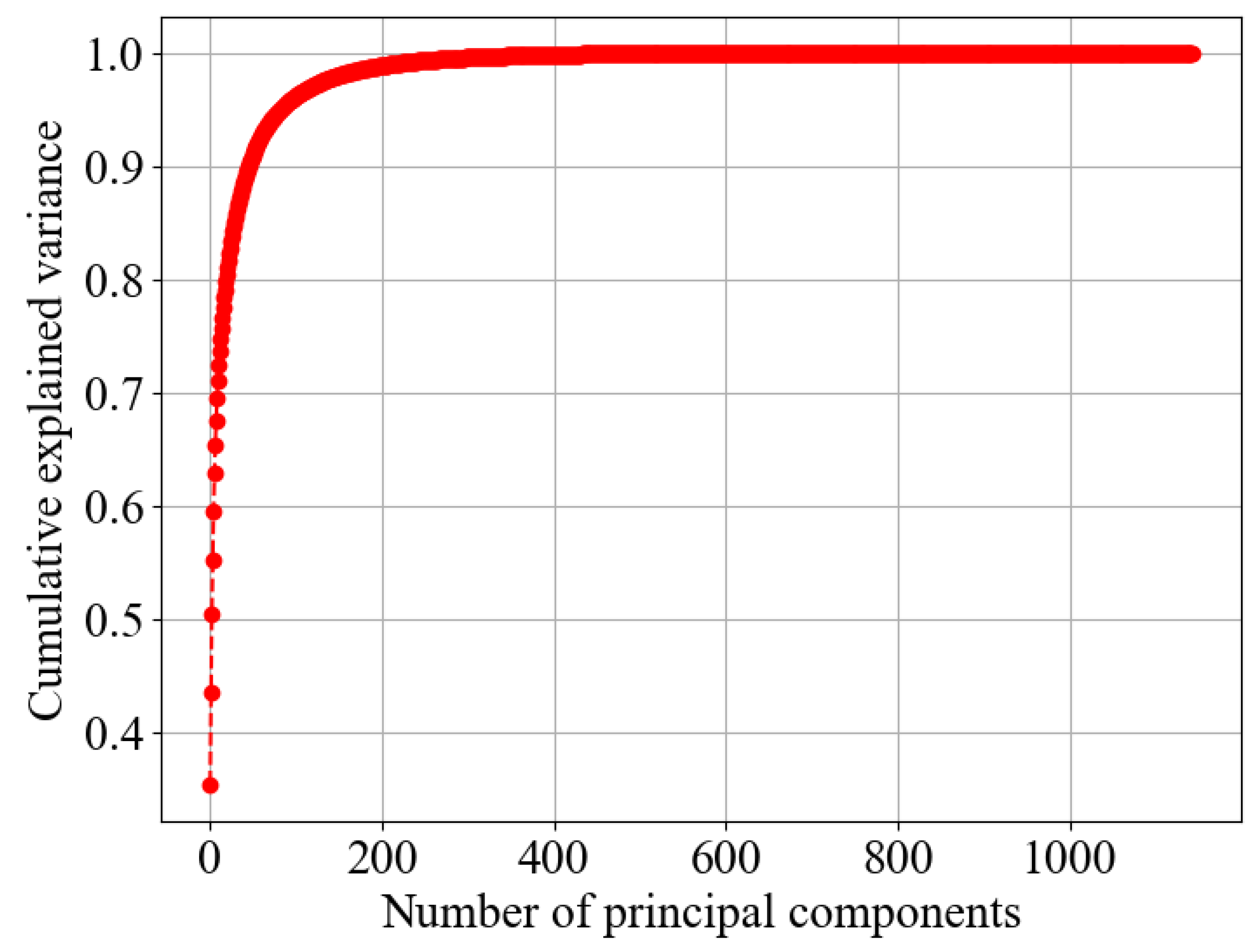
Therefore, the number of PCs was reduced by selecting the first eigenvectors in descending order of the eigenvalues. Additionally, the cumulative variance, as shown in Figure 5, was used to determine the optimal number of PCs needed to capture 99% of the variance in the mental disorder variables, ensuring that the reduced variables remain informative. In Figure 5, it can be observed that the curve starts to level off around 202 principal components (PCs), which explain 99% of the variance. This indicates that adding more PCs beyond this point results in only marginal increase in the cumulative explained variance. As a result, the total number of features was reduced from 1140 to 202, labeled PCA1–PCA202. See Section 4.3 and Section 4.4 for the biological relevance of the PCAs.

3.3.5. Data Splitting

To prepare the mental disorder data for model training and evaluation, a stratified three-way holdout split (80:10:10) was used with train_test_split from scikit-learn. Initially, an 80:20 split divided the dataset into training and test sets. Then, the test set was split again into validation and final test sets, each comprising 10% of the original data. This ensured the 80:10:10 ratio. Separate validation and test sets are crucial for robust model evaluation. The validation set assesses performance during training and hyperparameter tuning, guiding model selection and optimization. The final test set, held separately until the end, provides an unbiased evaluation of the model’s generalization ability on unseen data, simulating real-world applications. The training set was used for model training and hyperparameter tuning. The validation set monitors performance, helping to prevent overfitting and select optimal hyperparameters. The test set provided a final, independent assessment of the model’s ability to generalize to new, unseen mental disorder data.

3.4. Baseline Methods

In this section, we discuss the five baseline models used to compare the performance of the proposed model: kNN, ANN, LSTM, BiLSTM, and CNN-LSTM. Each model was implemented with both the PSD and FC features.

3.4.1. k-Nearest Neighbors (kNN)

The kNN model developed by Ahmed et al. [35], trained and tested on the same dataset as this study for a binary classification task (inherently easier than multiclass classification), was used as a baseline. Their proposed kNN architecture for mental disorder prediction was adapted for our multiclass classification task. The kNN algorithm operates by considering the k-closest data points to an input in the feature space, enabling it to capture decision boundaries and local patterns within the data. Its adaptability to diverse data characteristics and its intuitive mechanism make kNN suitable for mental disorder classification, as demonstrated by the comparative analysis in [35], thus establishing it as a relevant baseline for evaluating our proposed model’s performance.

3.4.2. Artificial Neural Network (ANN)

The ANN constructed by Ahmed et al. [35] for the binary classification task was modified in this study. It comprises interconnected layers that facilitate unidirectional information flow from the input layer to the output layer. The densely connected layers within the network process data via hidden units, enabling the model to learn patterns within the mental disorder data. The ANN architecture by [35] was chosen because of its proven performance. Comparative studies presented in [25] showed that their proposed ANN model outperforms other models in comparable contexts, specifically those involving mental disorder prediction and classification. This superior performance makes it a strong benchmark for evaluating the results of the present study.

3.4.3. Long Short-Term Memory (LSTM)

We modified the LSTM architecture developed by Ahmed et al. [35], originally designed for binary classification, to adapt it to our multiclass classification task. This architecture includes an input layer that accepts the vector representations of the mental disorder data, an LSTM layer that processes the data in one direction, a flatten layer that converts the data into a one-dimensional vector, a batch normalization layer, a dense layer that captures the pattern within the data, a dropout layer and an L2 regularizer that help prevent overfitting, and an output layer for predicting the mental disorder. We chose the LSTM method because of its ability to learn long-term dependencies within data. Comparative studies in [35] demonstrated that their model surpasses traditional mental disorder models in performance, establishing it as an effective benchmark for this study.

3.4.4. Bidirectional Long Short-Term Memory (BiLSTM)

The BiLSTM model developed by Ahmed et al. [35] for binary classification of mental disorders serves as a baseline in this study, which we modified for our multiclass classification task. Essentially, BiLSTM is an extended version of the LSTM architecture. It consists of two LSTM layers: one processes the data in a forward direction, from past to future, and the other processes it in a backward direction, from future to past, each with separate sets of hidden states and weights. BiLSTM was chosen as a baseline method because it incorporates bidirectional processing (forward and backward) at each time step, allowing the network to capture dependencies in both directions. Additionally, the BiLSTM model proposed by Ahmed et al. has demonstrated effectiveness in predicting mental disorders, providing a good benchmark for our study and enabling consistent and effective performance comparisons.

3.4.5. Convolutional Neural Network–Long Short-Term Memory (LSTM)

Building upon the established success of recurrent neural networks like BiLSTM in mental disorder classification, the CNN–LSTM architecture, exemplified by the model developed by Ahmed et al. [35] for binary classification, presents a compelling and robust baseline methodology. This architecture integrates the strengths of convolutional neural networks for feature extraction with the sequential modeling capabilities of LSTMs. By first employing convolutional layers, the model automatically learns local patterns and features from the input data, which are then fed into the LSTM layers to capture crucial long-range dependencies and temporal dynamics. This approach allows CNN–LSTM to move beyond simply processing sequential information, enabling it to identify and leverage intricate local features. Consequently, adapting and evaluating CNN–LSTM baseline for our multiclass classification task offers a powerful benchmark, potentially surpassing the capabilities of purely recurrent models by providing a richer, more context-aware representation of the complex patterns inherent in mental disorder data, thus facilitating a more rigorous evaluation of the proposed architecture.

3.5. Proposed CNN–BiLSTM Method

We developed a hybrid CNN–BiLSTM method to leverage the strengths of both architectures. The CNN acted as a local feature extractor, providing a more informative representation of the input data to the BiLSTM. This is particularly beneficial because of the high dimensionality of the mental disorder data. The BiLSTM captures long-range dependencies within the extracted features to improve the efficiency of the classifier. The hybrid classifier consists of an input layer, a convolutional layer, a pooling layer, a BiLSTM layer, and a concatenation layer, followed by a flatten layer, a dense layer with L2 regularization, a batch normalization layer, a dropout layer, and a prediction layer, as shown in Figure 6. These layers are further discussed in Section 3.5.1, Section 3.5.2, Section 3.5.3, Section 3.5.4, Section 3.5.5, Section 3.5.6, Section 3.5.7, Section 3.5.8.

3.5.1. Input Layer

The proposed method’s input layer receives the preprocessed sequence of mental disorder data. The resulting output is fed into the convolutional layer.

3.5.2. Convolutional Layer

To enhance accuracy in predicting mental disorders, a 1D convolutional layer is employed to extract local features. This layer employs convolutional filters to capture local patterns and dependencies within the input data. The rectified linear unit (ReLU) activation function is applied to improve the network’s learning dynamics and decrease the number of iterations required for convergence. Strides are then used to move the filter efficiently across the input data. The output of this layer is fed to the pooling layer.

3.5.3. Pooling Layer

Following the convolutional layer, a max pooling layer is applied to extract local features. This is achieved by taking the maximum value from a specified window of values in the input feature map. This value represents the most prominent feature within that region. The output of this layer is then passed to the BiLSTM layer.

3.5.4. BiLSTM Layer

After using the CNN layer to extract spatial features from the input data, the BiLSTM layer is then used to capture the long-range dependencies and relationships within the data. The BiLSTM layer consists of two LSTM cells: one LSTM cell processes the input sequence in a forward direction, and the second LSTM cell processes the input sequence in a backward direction. LSTM uses a gating mechanism, which consists of three gates: an input gate, a forget gate, and an output gate. The input gate controls the amount of the new input to be stored in the cell state. The forget gate controls the amount of the previous cell state that is forgotten. The output gate controls the amount of cell state to be outputted to the next time step. Given an input sequence X , the output of the LSTM unit at each time step (t) is expressed [42] in Equations (11)–(16) as
i t = σ ( W i X t + W h i h t 1 + b i )
f t = σ ( W f X t + W f h h t 1 + b f )
o t = σ ( W o X t + W o h h t 1 + b o )
q t = tanh ( W q X t + W q h h t 1 + b q )
c t = i t q t + f t c t 1
h t = o t tanh c t
In Equations (11)–(16), i , f , o , and c are the input gate, forget gate, output gate, and cell state, enumerated in time as i t , f t , o t , and c t , respectively. W , b , σ , tanh , and ⊗ represent the weight matrices, biases, softmax, hyperbolic target function, and element-wise multiplication, respectively. The outputs of these two LSTM networks are then concatenated to form the final output of the BiLSTM layer, as given by Equations (17)–(19):
h t = LSTM ( h t 1 , X T ) , t [ 1 , , T ]
z = ( h t h t )
where h t and t h n are the hidden layer states of the forward and backward BiLSTM. The output of the BiLSTM layer is then fed to the flatten layer.

3.5.5. Flatten Layer

The flatten layer reshapes the multi-dimensional output from the BiLSTM layer into a one-dimensional vector. This vector is fed as input to the dense layer.

3.5.6. Dense Layer

This layer learns the patterns between the mental disorders and their corresponding targets, creating more insightful representations. To reduce the complexity of the model and prevent overfitting, we applied an L2 regularization technique. This technique constrains the magnitude of the model’s weights, prevents it from memorizing the training data, and improves its ability to generalize to new data. This is achieved by adding a penalty term to the loss function that the model tries to minimize during training. This penalty is proportional to the square of the magnitude of the weights in the model. Given the original loss function ( L s ), the L2 loss function ( L r ) is given by Equation (20):
L r = L s + λ 2 x × w 2
where λ is the regularization strength, x represents the number of features, and w is the weight of the features.

3.5.7. Dropout Layer

To complement the L2 regularization technique in terms of addressing overfitting, we introduced a dropout layer. The dropout approach prevents the model from becoming too reliant on any individual unit by randomly dropping out some neurons based on the specified rate p r during training. This is achieved by setting the activations of the selected BiLSTM units to zero. For example, suppose the input vector from the dense layer is [ 0.7 , 1.2 , 3.0 , 2.1 , 0.2 , 0.6 ] and p r is 0.3. Thirty percent of the units are dropped, and the output vector is modified to [ 0.7 , 0 , 3.0 , 0 , 0.2 , 0.6 ] . This randomness forces the network to learn more robust features and reduce overfitting. The output from this layer is then fed into the prediction layer.

3.5.8. Prediction Layer

This layer effectively translates the learned features into specific, actionable predictions that are evaluated against the actual labels to assess the model’s performance. The output of this layer represents the probability of classifying mental disorders.

3.6. Hyperparameter Optimization

We optimized the proposed model by tuning the hyperparameters using a random search method within the training and validation sets of our three-way holdout split. This method was also applied to the five baseline models. Each iteration generated a model with different hyperparameter settings, fitted on the training data, and evaluated on the validation set. The chosen ranges for the hyperparameters were informed by existing studies and preliminary experiments, and the optimal hyperparameters were selected based on the performance on the validation set (accuracy).
For kNN, the number of neighbors was tuned using a search space (5, 6, 7, 8, or 9), and the optimal number was 9.
For the ANN, the number of neurons in hidden layers (16, 32, 64, or 96), learning rate (0.001, 0.0001, 0.00001, or 0.00002), optimizer (Adam or SGD), L2 regularizer rate (0.1, 0.01, 0.001, or 0.0001), dropout (0.2, 0.3, 0.4, or 0.5), and number of epochs (50, 100, or 150) were tuned. The optimal parameters were 16 neurons, the Adam optimizer, 150 epochs, an L2 regularizer rate of 0.01, a dropout of 0.3, and a learning rate of 0.001.
For LSTM and BiLSTM, the number of units (16, 32, 64, or 96), learning rate (0.001, 0.0001, 0.00001, or 0.00002), optimizer (Adam or SGD), L2 regularizer rate (0.1, 0.01, 0.001, or 0.0001), dropout (0.2, 0.3, 0.4, or 0.5), and epochs (50, 100, or 150) were tuned. The optimal parameters were 16 units, the Adam optimizer, 150 epochs, a learning rate of 0.0001, a dropout of 0.5, and an L2 regularizer rate of 0.001.
For the proposed CNN–LSTM method, the number of filters (16, 32, 64, or 96), kernel size (1, 2, or 3), LSTM units (16, 32, 64, or 96), learning rate (0.001, 0.0001, 0.00001, or 0.00002), optimizer (Adam or SGD), L2 regularizer rate (0.1, 0.01, 0.001, or 0.0001), dropout (0.2, 0.3, 0.4, or 0.5), and number of epochs (50, 100, or 150) were tuned. The optimal parameters were 16 filters, 16 LSTM units, a kernel size of 3, the Adam optimizer, 150 epochs, an L2 regularizer rate of 0.001, a dropout of 0.1, and a learning rate of 0.0001.
For the proposed CNN–BiLSTM method, the number of filters (16, 32, 64, or 96), kernel size (1, 2, or 3), BiLSTM units (16, 32, 64, or 96), learning rate (0.001, 0.0001, 0.00001, or 0.00002), optimizer (Adam or SGD), L2 regularizer rate (0.1, 0.01, 0.001, or 0.0001), dropout (0.2, 0.3, 0.4, or 0.5), and number of epochs (50, 100, or 150) were tuned. The optimal parameters were 16 BiLSTM units, a kernel size of 3, the Adam optimizer, 150 epochs, an L2 regularizer rate of 0.001, a dropout of 0.1, and a learning rate of 0.0001.

3.7. Model Training, Validation, and Testing: Proposed CNN–BiLSTM

The proposed CNN–BiLSTM model was configured with the optimal hyperparameters, and the model was compiled using the Adam optimizer with a specific learning rate, categorical cross-entropy loss, and accuracy metric. The model was trained on the training data, and its performance was evaluated on the validation set after each epoch using the loss rate and accuracy. Additionally, we assessed the model on unseen test set with standard metrics to ensure unbiased evaluation.

3.8. Performance Evaluation

The proposed CNN–BiLSTM and baseline methods were assessed using metrics such as accuracy ( A ), sensitivity (true positive rate ( TPR ) ) , specificity (false positive rate ( FPR ) ) , F1-score ( F ), and false negative rate ( FNR ) , as shown in Table 3.

3.9. Explanation of the Proposed Mental Disorder Model Prediction with LIME

LIME (local interpretable model-agnostic explanations) was employed to provide insights into the decision-making process of our CNN–BiLSTM model for individual predictions. The fundamental idea was to approximate the black-box model locally, in the vicinity of a specific instance, with a more interpretable model [43,44]. This allowed us to understand which features were the most influential for a particular prediction. The process began with perturbation: for a given mental disorder data instance, LIME generated a set of slightly altered neighboring samples. The nature and extent of these perturbations were determined based on the characteristics of the input features, aiming to explore the local decision boundary of the CNN–BiLSTM model.
These newly generated, perturbed data samples, along with the original instance, were then passed through the trained CNN–BiLSTM model to obtain their predictions. This created a local dataset of perturbed inputs and their corresponding model outputs. LIME used this local data to train an inherently interpretable surrogate model that aimed to approximate the CNN–BiLSTM model’s behavior, specifically around the instance being explained. To ensure local fidelity, LIME weighted the perturbed samples based on their proximity to the original instance. Samples closer to the original instance received higher weights, typically determined by a distance metric (e.g., Euclidean) and a kernel function (e.g., exponential) [43,44]. This weighted local dataset allowed the surrogate model to focus on explaining the CNN–BiLSTM model’s decision-making process in the immediate neighborhood of the prediction.
The importance of each input feature for the specific prediction was then derived from the parameters of the trained local surrogate model. For the linear surrogate model, the coefficients associated with each feature directly indicate its local importance. The absolute value of a coefficient reflects the strength of the feature’s influence on the prediction, while its sign indicates the direction of that influence (positive or negative). These feature weights, generated for each individual prediction, offer a localized and interpretable explanation of the CNN–BiLSTM model’s reasoning for that particular instance. The local surrogate model with an interpretability constraint is expressed mathematically as [43,44]:
E x p ( x ) = arg min q Q L ( p , q , π x ) + θ ( q )
where model q is the explanation model, for instance, x, and L denotes the loss minimized by model q. The loss L measures the closeness of the explanation to the original proposed CNN–BiLSTM model, denoted as p, while θ ( q ) represents the model’s complexity. Q represents the set of all possible explanations, and π x is the proximity measure that determines the size of the neighborhood around the instance x that was considered when creating an explanation for the model’s prediction.

3.10. Experimental Setup

The experiments were conducted in a Python 3.11.9 environment on a Windows 11 PC with a 13th-gen Intel Core i7-13650HX processor (2.60 GHz) and 16.0 GB of RAM. This configuration was employed to assess the method’s performance.

4. Results and Discussion

The experiments conducted in this study yielded insightful results that underscore the efficacy of our proposed mental disorder classifier. To provide a broad-spectrum analysis of mental disorders, this study employed a two-tiered classification approach. First, the model identified the main categories of mental disorders. Subsequently, it classified the specific disorders within these categories, offering detailed insights into their nuances. We implemented both the baseline methods and the hybrid CNN–BiLSTM model separately for both disorders using PSD and FC features. In this section, we present and analyze the key findings, illustrating the performance metrics and observed behaviors of the classifiers under various conditions.

4.1. Performance Comparison for the Main Disorders Using Evaluation Metrics: Proposed Method vs. Baseline Methods

We evaluated the proposed method and the baseline methods on the held-out test set using standard metrics, including accuracy, sensitivity, specificity, and F1-score. The results, summarized in Table 4, provide a quantitative assessment of each model’s ability to accurately classify mental disorders. The performance metrics reveal several important insights. kNN demonstrated the lowest performance across all metrics, suggesting its limited capacity to capture the complex patterns inherent in the mental disorder data. This underscores the necessity for more sophisticated DL architectures. ANN, LSTM, BiLSTM, and CNN-LSTM exhibited substantial improvements over kNN, indicating the value of nonlinear transformations and the ability to model temporal dependencies. Notably, LSTM achieved a slightly higher F1-score and accuracy than ANN and BiLSTM. Our proposed hybrid CNN–BiLSTM model exhibited the best performance across all metrics, achieving an accuracy of 76%, a sensitivity of 74%, a specificity of 76%, and an F1-score of 75%. This consistent performance across all metrics indicates the effectiveness of integrating convolutional layers for local feature extraction with the BiLSTM’s capability to model long-range dependencies. The CNN aids in identifying salient patterns within the input sequences, which are then effectively processed by the BiLSTM to capture temporal context, leading to improved classification accuracy and a better balance between precision and recall (as reflected in the F1-score). The modest but consistent improvement of CNN–BiLSTM over the BiLSTM baseline (accuracy increase of 6.5% and an F1-score increase of 9.3%) highlights the contribution of the convolutional component in enhancing the model’s discriminative power. While the BiLSTM alone captures significant sequential information, the CNN’s ability to extract relevant local features appears to provide complementary information that leads to more robust and accurate classification.

4.2. Receiver Operating Characteristic (ROC) Curve Analysis for the Main Disorders: Proposed Method vs. Baseline Methods

This section compares the performance of the baseline methods—kNN, ANN, LSTM, BiLSTM, CNN–LSTM, and the proposed CNN–BiLSTM method—using their receiver operating characteristic (ROC) curves. An ROC curve plots the true positive rate (TPR) against the false positive rate (FPR) at different classification thresholds. It helps assess and compare the diagnostic ability of the models. Each colored line on the graph in Figure 7 represents the ROC curve for a particular model. The black dashed diagonal line represents the performance of a random classifier (area under the curve (AUC) = 0.5). The AUC is a scalar value that summarizes the overall performance of each model. It represents the probability that the model will rank a randomly chosen positive instance higher than a randomly chosen negative instance. An AUC of 1.0 indicates a perfect mental disorder classifier, while an AUC of 0.5 indicates that the performance of the classifier is no better than random chance. The AUC for each model is shown in the legend. As seen in Figure 7, the CNN–BiLSTM model exhibited the best performance with the highest AUC of 0.91. ANN, BiLSTM, and CNN–LSTM also demonstrated good performance with AUCs of 0.89, 0.88, and 0.86, respectively, while kNN displayed a moderate level of discrimination with an AUC of 0.79, being the weakest among the models. Based on these findings, kNN may not be well suited for this classification task due to data complexity and high dimensionality. ANN performed better than kNN but was generally outperformed by LSTM, BiLSTM, and CNN–BiLSTM. This suggests that while ANNs can capture patterns, they may still struggle to handle complex data as effectively as other DL architectures. LSTM and BiLSTM demonstrated potential in processing high-dimensional and complex data. The superior performance of the proposed method can be attributed to the combination of a CNN for feature extraction and BiLSTM for capturing long-range dependencies. Furthermore, the proposed and baseline methods were evaluated using the FNR metric (Table 5). Lower FNR values indicate fewer missed cases. Analyzing the FNR for each model determines which one is more effective at minimizing missed disorder cases. The CNN–BiLSTM model had the lowest FNR for most disorders. For example, CNN–BiLSTM had an FNR of 7% for schizophrenia, suggesting it is more effective in diagnosing this disorder.

4.3. Performance Comparison for Specific Disorders Using Evaluation Metrics: Proposed Method vs. Baseline Methods

The proposed CNN–BiLSTM model demonstrated superior performance in the multiclass classification task for specific mental disorders on the held-out test set compared to the baseline methods, as shown in Table 6. Achieving an accuracy of 80% (2.5% higher than LSTM, the second best), a sensitivity of 77% (7.8% higher than the ANN, the lowest), a specificity of 80% (7.5% higher than CNN–LSTM), and an F1-score of 78% (6.4% higher than BiLSTM), it outperformed kNN (lowest), ANN, LSTM, BiLSTM, and CNN–LSTM. This improvement highlights the effectiveness of combining the CNN’s local feature extraction with BiLSTM’s temporal modeling for capturing complex patterns within the data, leading to more accurate and balanced classification of specific mental disorder categories.

4.4. Performance Comparison of the Proposed and Baseline Methods for Specific Disorders Based on Their ROC Curves

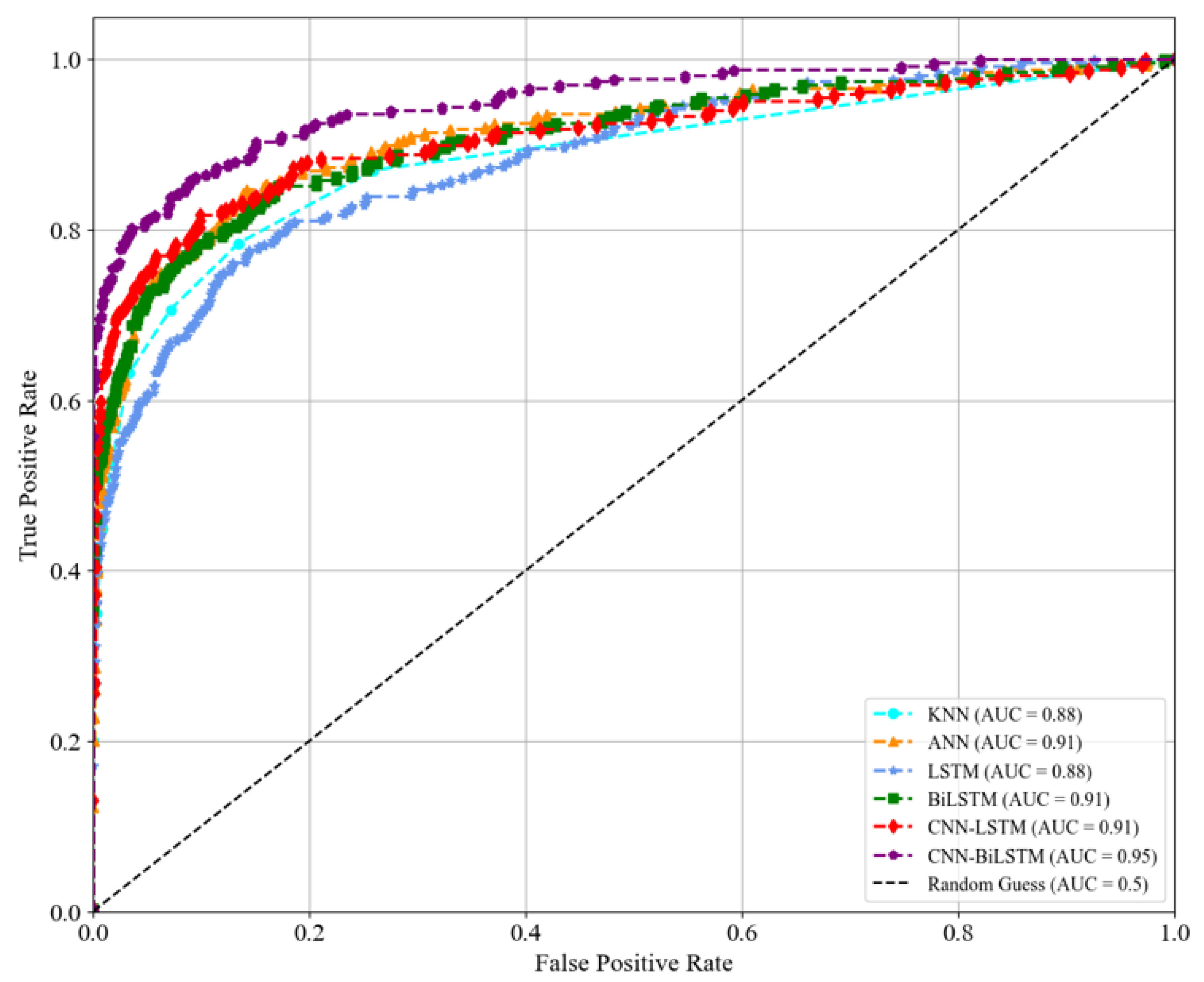
The ROC curves in this section were used to provide a visual assessment of the performance of the proposed and baseline methods for specific disorders using the same PSD and FC features used for the main disorders. This assessment offers a detailed view of the trade-off between sensitivity and specificity for each method. As shown in Figure 8, the proposed CNN–BiLSTM model achieved the highest AUC of 0.95, demonstrating its superior classification performance for specific disorders. ANN, BiLSTM, and CNN–LSTM exhibited strong and comparable performance with AUCs of 0.91. kNN and LSTM had slightly lower yet still substantial discriminatory ability, with AUCs of 0.88. The consistently high AUC values across all models suggest a strong potential for accurate classification within specific disorders. The proposed CNN–BiLSTM model’s marginal but noticeable improvement indicates the effectiveness of the architecture in capturing relevant patterns within the data for this specific task. Moreover, the proposed and baseline methods were assessed using the FNR metric, as illustrated in Table 7. These results demonstrate that the CNN–LSTM and CNN–BiLSTM models exhibited lower FNR values across the specific disorders, suggesting higher efficiency in correctly diagnosing these conditions.

4.5. Impact of kNN Data Imputation on the Performance of CNN-BiLSTM in Classifying Mental Disorders

This study investigates the impact of the kNN imputation method on the CNN–BiLSTM model’s performance in multiclass mental disorder classification. Table 8 and Table 9 present an ablation-style comparison, showing the model’s results with and without kNN imputation for the main disorders and specific disorders, respectively. Performance was evaluated using accuracy, sensitivity, specificity, and F1-score.
For both the main and specific disorders, the results indicate that kNN imputation improved the CNN–BiLSTM model’s performance across all metrics. Specifically, for the main disorders (Table 8), accuracy improved from 70% to 76%, sensitivity from 68% to 74%, specificity from 70% to 76%, and the F1-score from 67% to 75% when kNN imputation was applied. Similarly, for specific disorders (Table 9), accuracy improved from 78% to 80%, specificity from 78% to 80%, and the F1-score from 74% to 78% with kNN imputation. This ablation study provides evidence that kNN imputation is a valuable preprocessing step for the CNN–BiLSTM model in this context. By imputing missing values, the model achieves better overall performance in classifying both main and specific mental disorder categories.

4.6. Impact of PCA on the Performance of CNN–BiLSTM in Classifying Mental Disorders

This section investigates the impact of PCA on the proposed CNN–BiLSTM model’s performance by comparing the results obtained with and without its application to both the main and specific disorders. The results, assessed across specific evaluation metrics—accuracy, sensitivity, specificity, and F1-score—are presented in Table 10 and Table 11.
For the main disorders (Table 10), PCA yielded a clear positive impact on the CNN–BiLSTM model’s performance. Accuracy and specificity both increased by approximately 11% (from 68% to 76%), while the F1-score saw a considerable rise of 17% (from 62% to 75%). Although sensitivity experienced a minor decrease (from 76% to 74%), the substantial gains across other metrics suggest that PCA effectively enhanced the discriminative power for these broader disorder categories by retaining relevant information despite dimensionality reduction.
Regarding specific disorders (Table 11), PCA still demonstrated a positive impact on the performance of the proposed CNN–BiLSTM model. Accuracy and specificity showed improvements of approximately 3% (from 78% to 80%), and the F1-score improved by 1% (from 77% to 78%). Sensitivity decreased by 1% (from 78% to 77%). These results indicate that PCA did not negatively affect the classification of this category but contributed to a slight refinement by potentially mitigating noise. Based on these findings, the application of PCA generally improved the CNN–BiLSTM model’s performance on both the main and specific disorder datasets. The more substantial gains observed for the main disorders suggest that PCA was particularly effective in optimizing the feature space for these broader classifications. The consistent positive trend supports the use of PCA as a beneficial dimensionality reduction technique for this mental disorder multiclass classification task.

4.7. Impact of Different Loss Functions on the FNR ( % ) of the Proposed Model for Specific Disorders

This section presents a comparative analysis of the impact of the cross-entropy, weighted categorical cross-entropy, and focal loss functions on the FNR of our proposed model across various specific disorders, as detailed in Table 12. Our observations revealed distinct performance patterns for each loss function. Specifically, the cross-entropy loss function yielded low FNR values for acute stress disorder (3%), alcohol use disorder (12%), behavioral disorder (16%), and panic disorder (7%). However, it exhibited a considerably higher FNR of 40% for depressive disorder. In contrast, the weighted categorical cross-entropy loss function demonstrated efficacy for adjustment disorder (4%), bipolar disorder (4%), post-traumatic stress disorder (6%), and social anxiety disorder (11%) but resulted in a notably high FNR of 58%. Similarly, the focal loss function achieved low FNR values for adjustment disorder (4%), bipolar disorder (4%), and social anxiety disorder (7%), while also showing a high FNR of 55% for depressive disorder. Notably, among the three loss functions, categorical cross-entropy resulted in the lowest FNR (40%) for depressive disorder. The relatively high FNR values observed for certain disorders, particularly depressive disorder, suggest inherent complexities and feature overlap that pose challenges for classification. Despite these difficulties, our proposed CNN–BiLSTM model consistently achieved lower FNR values than the baseline methods, indicating its improved ability to discern these challenging data characteristics. These findings highlight the sensitivity of model performance to the choice of loss function and underscore the need for careful consideration based on the specific characteristics of the disorders being classified.

4.8. Interpreting the Proposed Model’s Decisions Using LIME for the Main Disorders

To enhance the decision-making process of the CNN–BiLSTM model for addictive disorders, particularly concerning the neurobiological relevance of the contributing features, we employed LIME. LIME approximates the complex, nonlinear model locally around individual predictions with an interpretable linear model, thereby revealing the features that most significantly influence the output for a specific instance. Figure 9 presents the LIME results for a case where the model predicted addictive disorders with a high probability of 0.89. The local linear approximation indicated that positive values of specific principal components (PCs), notably PCA40 and PCA29, exerted a positive influence on this prediction, increasing the likelihood of the “addictive” classification for this instance. Additionally, PCA175 also contributed positively, albeit with a smaller coefficient in the local linear model. Conversely, negative values of PCs such as PCA8 and PCA38 exhibited a negative influence, decreasing the likelihood of the “addictive” prediction for this case.
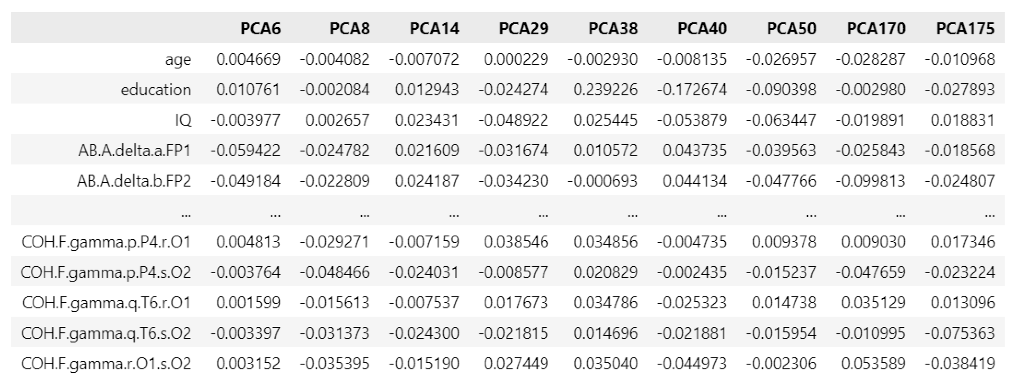
To establish a biological interpretation between the abstract principal components and the underlying neurophysiological data, we refer to the PCA loading matrix presented in Figure 10). The loadings represent the coefficients of the linear combination of the original EEG features (e.g., power in specific frequency bands across different channels, or functional connectivity measures between electrode pairs) and demographic features that constitute each PC, indicating the strength and direction of each original feature’s contribution to the component’s variance. For instance, the PCA loading matrix revealed that PCA40 was positively associated with the delta power at the frontal pole electrodes FP1 (AB.A.delta.a.FP1 = 0.043735) and FP2 (AB.A.delta.b.FP2 = 0.044134). Furthermore, PCA29 exhibited positive loadings for gamma-band coherence between parietal electrode P4 and occipital electrode O1 (COH.F.gamma.p.P4.r.O1 = 0.038546), gamma-band coherence between temporal electrode T6 and occipital electrode O1 (COH.F.gamma.q.T6.r.O1 = 0.017673), and gamma-band coherence between occipital electrodes O1 and O2 (COH.F.gamma.r.O1.s.O2 = 0.027449). According to the LIME results, the presence of increased delta activity in the frontal regions and enhanced gamma-band synchronization within occipital-parietal and occipital-temporal networks in this individual’s EEG data contributed to the model’s prediction of addictive disorder. Conversely, PCA8 showed a weak positive loading for IQ (0.002657), suggesting a minimal direct opposing influence from this demographic variable in this specific instance. PCA38, which negatively influenced the prediction, exhibited positive loadings for education (0.239226), IQ (0.025445), delta power at FP1 (AB.A.delta.a.FP1 = 0.010572), and the gamma coherence measures (COH.F.gamma.p.P4.r.O1 = 0.034856, COH.F.gamma.p.P4.s.O2 = 0.020829, COH.F.gamma.q.T6.r.O1 = 0.034786, COH.F.gamma.q.T6.s.O2 = 0.014696, COH.F.gamma.r.O1.s.O2 = 0.035040). This indicates that lower values in these original features for this specific instance contributed to opposing the addictive disorder prediction. By establishing this mapping between the influential PCs identified by LIME and their constituent original EEG and demographic features via the PCA loading matrix, we provide a more transparent and potentially clinically interpretable understanding of the model’s decision-making process. This approach moves beyond the inherent abstractness of dimensionality reduction techniques and offers a crucial step toward linking the model’s predictions to underlying biological mechanisms relevant to addictive disorders.
The LIME results for anxiety disorders (Figure 11) revealed that the model’s prediction of anxiety disorders with a high probability of 98% was primarily driven by a high positive value in PCA24 (feature value = 2.29) and a negative value in PCA146 (feature value = −0.42). These feature values, relative to the thresholds identified by LIME (PCA24 > 1.63 and PCA146 <= −0.26), positively contributed to the classification of anxiety disorders for this specific instance. Conversely, the prediction was opposed by a negative value in PCA2 (feature value = −7.18, where PCA2 <= −5.38 decreased the probability of anxiety disorders) and a negative value in PCA1 (feature value = −1.17, where −3.87 < PCA1 <= 1.35 decreased the probability).
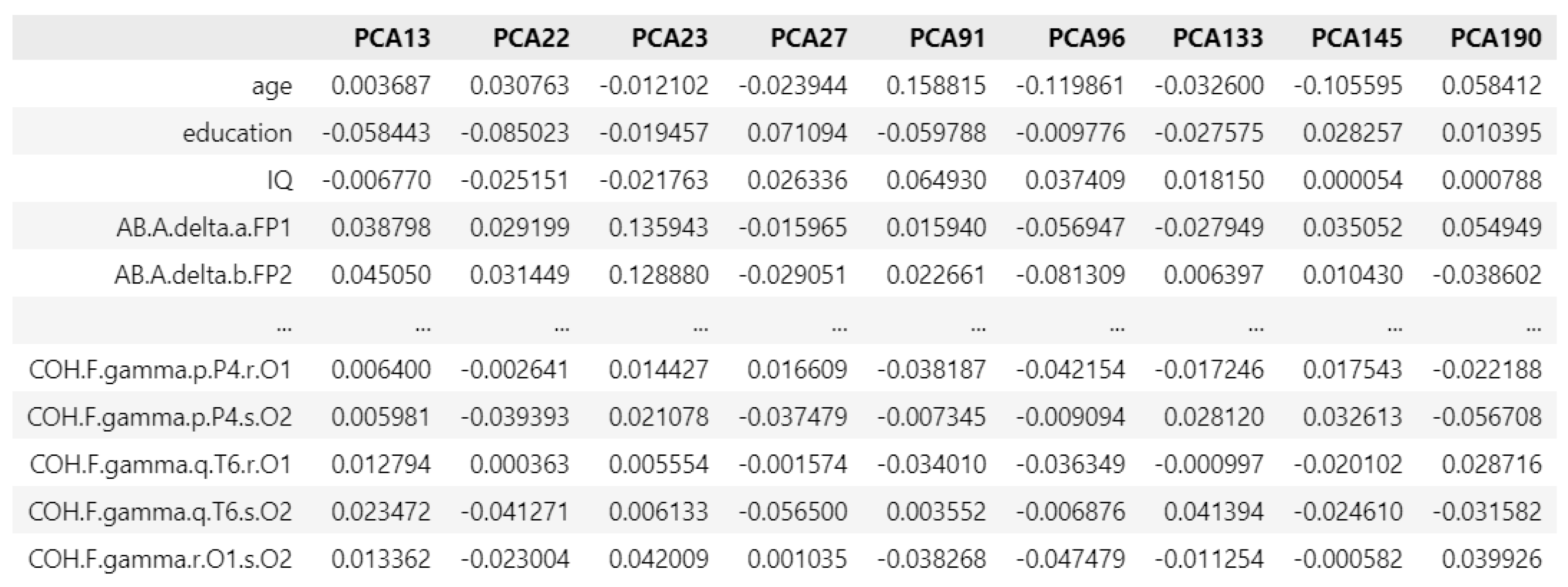
For instance, the PCA loading matrix in Figure 12 reveals that PCA24 exhibited a moderate negative loading for age = −0.042086 and a positive loading for IQ = 0.022447. It also shows small positive loadings for AB.A.delta.a.FP1 = 0.023321, AB.A.delta.b.FP2 = 0.030999, and COH.F.gamma.q.T6.r.O1 = 0.002232. Furthermore, PCA146 shows a small positive loading for age = 0.034930 and for education = 0.043531. It also exhibits a small positive loading for AB.A.delta.a.FP1 = 0.004206. Additionally, it shows a moderate positive loading for gamma-band coherence between parietal electrode P4 and occipital electrode O2 (COH.F.gamma.p.P4.s.O2 = 0.055320). PCA2 exhibits a small positive loading for age = 0.001821 and a moderate positive loading for education = 0.01229. It also shows a small negative loading for AB.A.delta.a.FP1 = −0.000314, a small positive loading for AB.A.delta.b.FP2 = 0.001175, and a small negative loading for gamma-band coherence between parietal electrode P4 and occipital electrode O1 (COH.F.gamma.p.P4.r.O1 = −0.0273). Furthermore, PCA1 shows a very small positive loading for age = 0.000066 and for education = 0.002002. It also exhibits a small positive loading for AB.A.delta.a.FP1 = 0.003863 and a moderate positive loading for COH.F.gamma.p.P4.r.O1 = 0.031681. By examining the loadings of these principal components, we understand how combinations of original demographic and EEG features contribute to the variance captured by each component. LIME identifies these PCs as important for predicting anxiety disorders, so we can then infer that the specific patterns of these underlying features are influential in the model’s decision-making process. For example, a high positive value in PCA24, which has a positive loading for IQ, suggests that individuals with higher IQ scores exhibit a pattern of brain activity and demographics that the model associates with anxiety, although the negative loading for age also plays a role. Similarly, the negative influence of PCA146, which has a negative loading for certain functional connectivity measures, indicates that lower levels of that specific synchronization pattern are associated with the model’s anxiety disorder prediction.
In Figure 13, the LIME results indicate that the model predicted obsessive disorders with a high probability of 98%. This prediction was primarily driven by high positive values in PCA8 (feature value = 3.19, where PCA8 > 1.62 increased the probability) and PCA9 (feature value = 2.20, where PCA9 > 2.17 increased the probability). Positive values in PCA22 (feature value = 2.38, where PCA22 > 1.25 increased the probability) and PCA38 (feature value = 1.12, where PCA38 > 0.97 increased the probability) also contributed to this classification. Conversely, the model’s prediction was opposed by negative values in PCA23 (feature value = −2.94, where PCA23 <= −1.29 decreased the probability), PCA20 (feature value = −1.62, where PCA20 <= −1.43 decreased the probability), and PCA21 (feature value = −4.19, where PCA21 <= −1.23 decreased the probability). A negative value in PCA25 (feature value = −2.08, where PCA25 <= −1.04 decreased the probability) also opposed the “obsessive” classification.
In the PCA loading matrix in Figure 14, PCA8 exhibits a small negative loading for age = −0.004082 and a very small negative loading for education = −0.002084. It shows a very small positive loading for IQ = 0.002657 and a small negative loading for AB.A.delta.a.FP1 = −0.024782. It also displays a moderate negative loading for COH.F.gamma.p.P4.r.O1 = −0.029271. PCA9 shows a very small positive loading for age = 0.002786 and for education = 0.001721. It exhibits a moderate negative loading for IQ = −0.010832 and a moderate positive loading for AB.A.delta.a.FP1 = 0.023589. It also displays a small negative loading for COH.F.gamma.p.P4.r.O1 = −0.010475. PCA38 exhibits a moderate positive loading for education = 0.239226 and a small positive loading for IQ = 0.025445. It shows a small positive loading for AB.A.delta.a.FP1 = 0.010572 and for COH.F.gamma.p.P4.r.O1 = 0.034856. PCA22 shows a small positive loading for age = 0.030763 and a moderate negative loading for education = −0.085023. It exhibits a moderate negative loading for IQ = −0.025151 and a moderate positive loading for AB.A.delta.a.FP1 = 0.029199. It also displays a very small negative loading for COH.F.gamma.p.P4.r.O1 = −0.002641. For the negatively contributing components, PCA23 exhibits a small negative loading for age = −0.012102 and for education = −0.019457. It shows a small negative loading for IQ = −0.021763 and a moderate positive loading for AB.A.delta.a.FP1 = 0.135943. It also displays a small positive loading for COH.F.gamma.p.P4.r.O1 = 0.014427. PCA20 shows a very small positive loading for age = 0.008371 and a small negative loading for education = −0.037366. It exhibits a small negative loading for IQ = −0.010764 and a small positive loading for AB.A.delta.a.FP1 = 0.015537. It also displays a moderate negative loading for COH.F.gamma.p.P4.r.O1 = −0.030891. PCA21 exhibits a small positive loading for age = 0.020084 and a moderate negative loading for education = −0.060763. It shows a small negative loading for IQ = −0.013818 and a very small positive loading for AB.A.delta.a.FP1 = 0.003533. It also displays a small positive loading for COH.F.gamma.p.P4.r.O1 = 0.015709. PCA25 shows a small positive loading for age = 0.020656 and for education = 0.012669. It exhibits a small positive loading for IQ = 0.012639 and for AB.A.delta.a.FP1 = 0.018693. It also displays a very small positive loading for COH.F.gamma.p.P4.r.O1 = 0.003872.

4.9. Interpreting the Proposed Model’s Decisions Using LIME for Specific Disorders

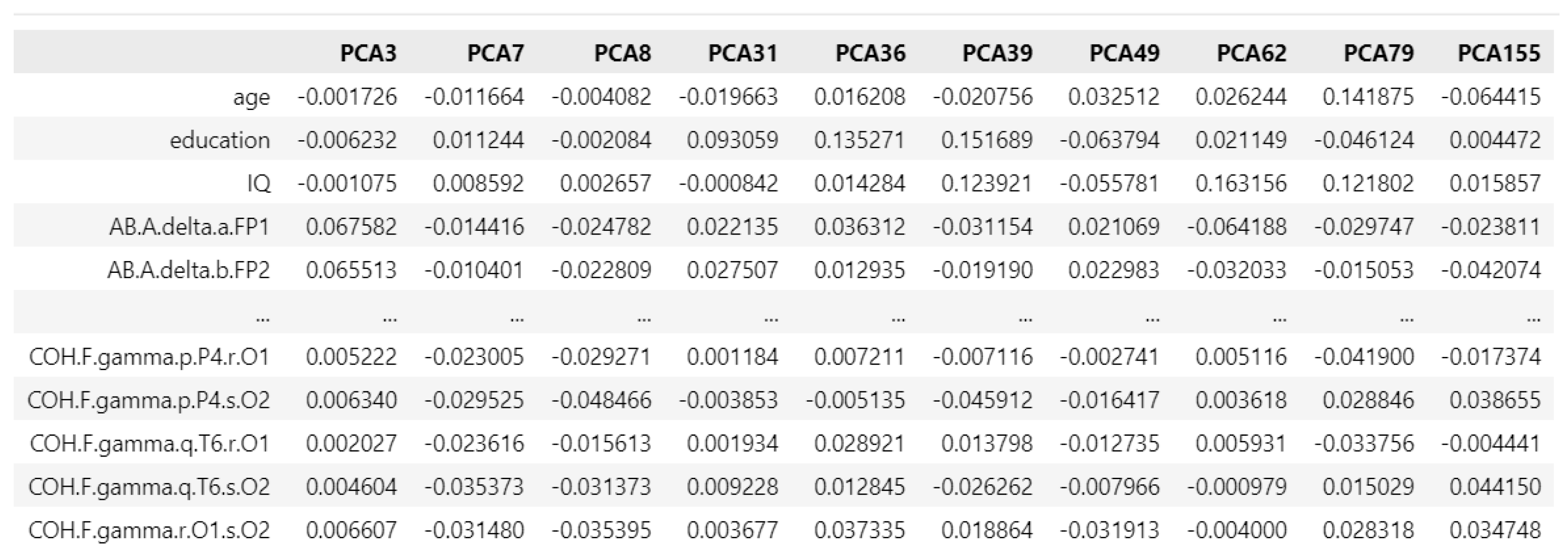
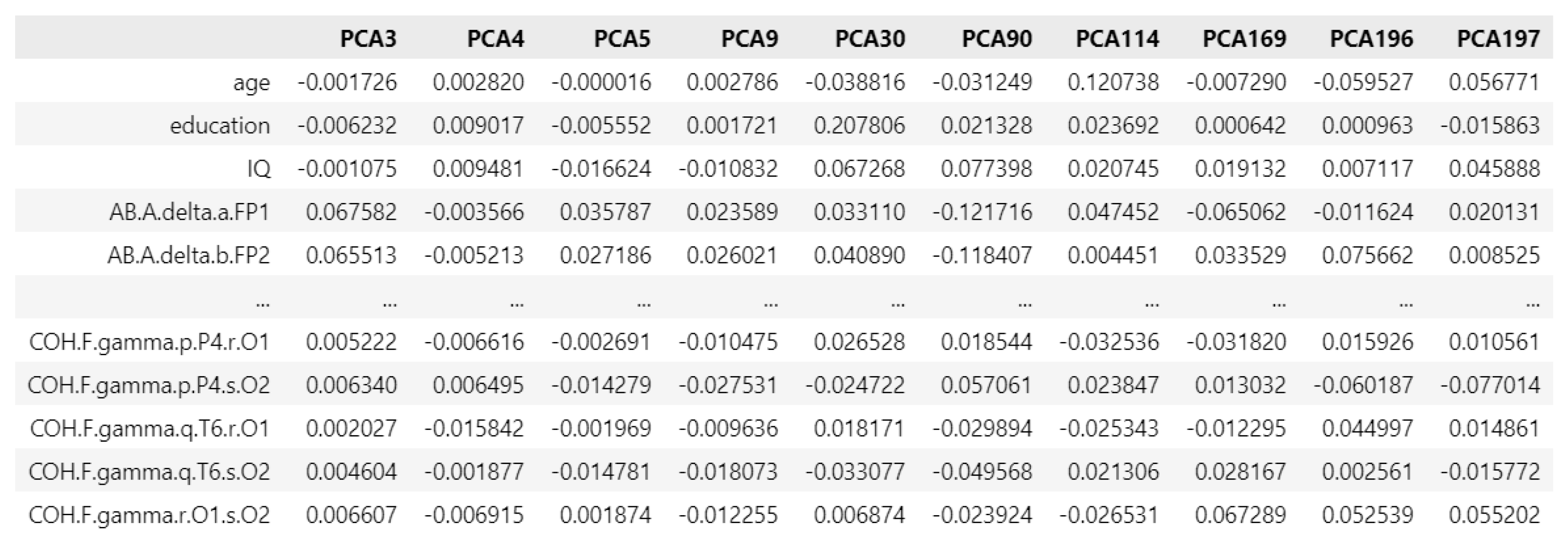
We examined the interpretability of the proposed model’s decisions regarding specific disorders using LIME. As shown in Figure 15, the model predicted acute disorders with a probability of 91%. The local linear approximation revealed that this prediction was primarily driven by a high positive value in PCA3 (feature value = 9.41, where PCA3 > 3.74 increased the probability). Positive values in PCA79 (feature value = 0.97, where PCA79 > 0.62 increased the probability) and PCA36 (feature value = −1.85, where PCA36 <= −0.98 increased the probability) also contributed to this classification. The model’s decision was opposed by negative values, including PCA39 (feature value = −1.14, where PCA39 <= −0.77 decreased the probability), PCA8 (feature value = −6.01, where PCA8 <= −2.77 decreased the probability), and PCA7 (feature value = −2.29, where PCA7 <= −2.25 decreased the probability). Negative feature values in these components decreased the likelihood of the “acute stress” prediction for this specific case. To understand the biological relevance of these PCA components, their loadings on the original EEG and demographic features, as detailed in the PCA loading matrix in Figure 16, were examined.
In the PCA loading matrix in Figure 16, PCA3 shows positive loadings for delta power at FP1 and FP2 (AB.A.delta.a.FP1 = 0.067582 and AB.A.delta.b.FP2 = 0.065513) and weak positive loadings for specific gamma-band coherence (COH.F.gamma.p.P4.r.O1 = 0.005222; COH.F.gamma.p.P4.s.O2 = 0.006340; COH.F.gamma.q.T6.r.O1 = 0.002027; COH.F.gamma.q.T6.s.O2 = 0.004604; and COH.F.gamma.r.O1.s.O2 = 0.006607). PCA7 exhibits positive loadings for education (0.011244) and weak positive loadings for IQ (0.008592). It also shows negative loading for age (−0.001726), delta power at FP1 and FP2 (AB.A.delta.a.FP1 = −0.014416 and AB.A.delta.b.FP2 = −0.010401), and gamma-band coherence (COH.F.gamma.p.P4.r.O1 = −0.023005; COH.F.gamma.p.P4.s.O2 = −0.029525; COH.F.gamma.q.T6.r.O1 = −0.023616; COH.F.gamma.q.T6.s.O2 = −0.035373; and COH.F.gamma.r.O1.s.O2 = −0.031480). PCA8 displays a positive loading only for IQ (0.002657). It displays negative loadings for age (−0.004082), education (−0.002084), delta power FP1 and FP2 (AB.A.delta.a.FP1 = −0.024782 and AB.A.delta.b.FP2 = −0.022809), and gamma-band coherence (COH.F.gamma.p.P4.r.O1 = −0.029271; COH.F.gamma.p.P4.s.O2 = −0.048466; COH.F.gamma.q.T6.r.O1 = −0.015613; COH.F.gamma.q.T6.s.O2 = −0.031373; and COH.F.gamma.r.O1.s.O2 = −0.035395). PCA31 shows positive loadings for education (0.093059) and delta power at FP1 and FP2 (AB.A.delta.a.FP1 = 0.022135 and AB.A.delta.b.FP2 = 0.027507) and weak positive loadings for specific gamma-band coherence (COH.F.gamma.p.P4.r.O1 = 0.001184; COH.F.gamma.q.T6.r.O1 = 0.001934; COH.F.gamma.q.T6.s.O2 = 0.009228; and COH.F.gamma.r.O1.s.O2 = 0.003677). PCA36 exhibits negative loadings only for a specific gamma-band coherence (COH.F.gamma.p.P4.s.O2 = −0.003853), while age, education, IQ, AB.A.delta.a.FP1, AB.A.delta.b.FP2, COH.F.gamma.p.P4.r.O1, COH.F.gamma.q.T6.r.O1, COH.F.gamma.q.T6.s.O2, and COH.F.gamma.r.O1.s.O2 have positive loadings. PCA39 shows positive loadings for education (0.151689), IQ (0.123921), COH.F.gamma.q.T6.r.O1 (0.013798), and COH.F.gamma.r.O1.s.O2 (0.013798), while age, AB.A.delta.a.FP1, AB.A.delta.a.FP2, COH.F.gamma.p.P4.r.O1, COH.F.gamma.p.P4.s.O2, and COH.F.gamma.q.T6.s.O2 have negative loadings. PCA79 shows strong positive loadings for age (0.141875) and IQ (0.121802), while it shows negative loadings for education, AB.A.delta.a.FP1, AB.A.delta.a.FP2, COH.F.gamma.p.P4.r.O1, and COH.F.gamma.q.T6.r.O1.
In Figure 17, the LIME results reveal that the proposed model strongly predicted post-traumatic stress disorder with a high probability of 92%. The local linear approximation revealed that the strong prediction was primarily driven by high positive values in PCA3 (feature value = 6.13, where PCA3 > 3.74 increased the probability) and PCA30 (feature value = 2.68, where PCA30 > 0.91 increased the probability). Moreover, the model’s decision was opposed by negative values like PCA5 (feature value = −6.07, where PCA5 <= −3.04 decreased the probability) and PCA4 (feature value = −9.14, where PCA4 <= −4.38 decreased the probability). The PCA loading matrix that mapped the important PCA features identified by the LIME method for post-traumatic stress disorder in Figure 17 is provided in Figure 18.
In Figure 19, the LIME results indicate that the model strongly predicted alcohol use disorder with a probability of 96%. This high prediction could be attributed to the high positive value in PCA13 (feature value = 2.97, where PCA13 > 2.08 increased the probability). Positive values in PCA91 (feature value = 0.43, where PCA91 > 0.41 increased the probability) and PCA35 (feature value = 1.05, where PCA35 > 1.01 increased the probability) also contributed to this classification. However, the model’s prediction was strongly opposed by a negative value in PCA145 (feature value = −0.83, where PCA145 <= −0.31 decreased the probability). Negative values in PCA22 (feature value = −4.27, where PCA22 <= −1.14 decreased the probability), PCA23 (feature value = −3.88, where PCA23 <= −1.34 decreased the probability), and PCA27 (feature value = −1.88, where PCA27 <= −1.17 decreased the probability) also acted against the prediction of alcohol use disorder. The influence of PCA190 (feature value = 0.20, where PCA190 > −0.19 increased the probability) and PCA96 (feature value = 0.65, where PCA96 > −0.44 increased the probability) was positive but less dominant. PCA133 (feature value = 0.33, where PCA33 > 0.27 increased the probability) also showed a small positive contribution. For enhanced interpretability of the LIME results for post-traumatic stress disorder presented in Figure 19, the PCA loading matrix, mapping the key PCs to the original features, is provided in Figure 20.

5. Limitations

In this study, single-institutional data were used to develop the proposed CNN–BiLSTM model for assessing patients with mental disorders. While the promising results of the proposed model demonstrate its effectiveness for mental disorder diagnosis across different conditions, the model may have limited generalizability to broader populations or other clinical settings. To mitigate this limitation, future work will focus on validating our findings using multi-center datasets to assess the robustness and generalizability of the developed model across diverse populations and settings.

6. Conclusions

In this study, we proposed a hybrid CNN–BiLSTM model to predict mental disorders in patients. To enhance the model’s performance, we addressed issues related to missing data using the kNN imputation method, and class imbalance was mitigated using SMOTE. PCA was utilized to reduce dimensionality and enhance the prediction accuracy of the mental disorder model. Additionally, the LIME method was implemented to interpret model predictions, addressing the black-box problem typically associated with complex mental disorder models. The outcomes of this study enhance the understanding and trustworthiness of DL models for clinicians and researchers, contributing to more reliable and interpretable mental disorder predictions.

Author Contributions

Conceptualization, D.O., A.A.-M. and H.M.; Data curation, D.O.; Formal analysis, D.O., A.A.-M. and H.M.; Funding acquisition, A.A.-M. and H.M.; Investigation, D.O., A.A.-M. and H.M.; Methodology, D.O., A.A.-M. and H.M.; Project administration, A.A.-M. and H.M.; Resources, A.A.-M. and H.M.; Software, D.O.; Validation, D.O., A.A.-M. and H.M.; Visualization, D.O., A.A.-M. and H.M.; Writing—original draft, D.O.; Writing—review and editing, D.O., A.A.-M. and H.M. All authors have read and agreed to the published version of the manuscript.

Funding

This research work was supported by the Council for Scientific and Industrial Research, Pretoria, South Africa, through the Smart Networks collaboration initiative and IoT-Factory Program (funded by the Department of Science and Innovation (DSI), South Africa).

Institutional Review Board Statement

Not applicable.

Informed Consent Statement

Informed consent was obtained from all subjects involved in this study.

Data Availability Statement

The dataset we used is available at https://osf.io/8bsvr/(accessed on 10 November 2024).

Conflicts of Interest

The authors declare that there are no conflicts of interest and that the funders had no role in the design of the study; in the collection, analyses, or interpretation of data; in the writing of the manuscript, or in the decision to publish the results.

References

  1. Jauhar, S.; Johnstone, M.; McKenna, P.J. Schizophrenia. Lancet 2022, 399, 473–486. [Google Scholar] [CrossRef] [PubMed]
  2. Xu, Y.; Zhong, H.; Ying, S.; Liu, W.; Chen, G.; Luo, X. Depressive disorder recognition based on frontal EEG signals and deep learning. Sensors 2023, 23, 8639. [Google Scholar] [CrossRef]
  3. Cai, H.; Qu, Z.; Li, Z.; Zhang, Y.; Hu, X.; Hu, B. Feature-level fusion approaches based on multimodal EEG data for depression recognition. Inf. Fusion 2020, 59, 127–138. [Google Scholar] [CrossRef]
  4. McCarron, R.M.; Shapiro, B.; Rawles, J.; Luo, J. Depression. Ann. Intern. Med. 2021, 174, 65–80. [Google Scholar] [CrossRef] [PubMed]
  5. Olatinwo, D.D.; Abu-Mahfouz, A.; Hancke, G.; Myburgh, H. IoT-enabled WBAN and machine learning for speech emotion recognition in patients. Sensors 2023, 23, 2948. [Google Scholar] [CrossRef]
  6. Szuhany, K.L.; Simon, N.M. Anxiety disorders: A review. JAMA 2022, 24, 2431–2445. [Google Scholar] [CrossRef]
  7. Zhang, C.; Xiao, X.; Li, T.; Li, M. Translational genomics and beyond in bipolar disorder. Mol. Psychiatry 2021, 23, 186–202. [Google Scholar] [CrossRef]
  8. Costello, E.J. Early detection and prevention of mental health problems: Developmental epidemiology and systems of support. J. Clin. Child Adolesc. Psychol. 2016, 45, 710–717. [Google Scholar] [CrossRef]
  9. Obeid, S.; Hallit, C.A.; Haddad, C.; Hany, Z.; Hallit, S. Validation of the Hamilton Depression Rating Scale (HDRS) and sociodemographic factors associated with Lebanese depressed patients. L’encephale 2018, 5, 397–402. [Google Scholar] [CrossRef]
  10. You, C.; Shen, Y.; Sun, S.; Zhou, J.; Li, J.; Su, G.; Michalopoulou, E.; Peng, W.; Gu, Y.; Guo, W.; et al. Artificial intelligence in breast imaging: Current situation and clinical challenges. InExploration 2023, 5, 20230007. [Google Scholar] [CrossRef]
  11. Li, C.; Wang, T.; Zhou, S.; Sun, Y.; Xu, Z.; Xu, S.; Shu, S.; Zhao, Y.; Jiang, B.; Xie, S.; et al. Deep learning model coupling wearable bioelectric and mechanical sensors for refined muscle strength assessment. Research 2024, 23, 0366. [Google Scholar] [CrossRef] [PubMed]
  12. Yi, N.; Zhang, C.; Wang, Z.; Zheng, Z.; Zhou, J.; Shang, R.; Zhou, P.; Zheng, C.; You, M.; Chen, H.; et al. Multi-Functional Ti3C2Tx-Silver@ Silk Nanofiber Composites with Multi-Dimensional Heterogeneous Structure for Versatile Wearable Electronics. Adv. Funct. Mater. 2025, 35, 2412307. [Google Scholar] [CrossRef]
  13. Qi, R.; Zou, Q. Trends and potential of machine learning and deep learning in drug study at single-cell level. IEEE Res. 2023, 9, 0050. [Google Scholar] [CrossRef]
  14. Cruz, J.A.; Marquez, J.C.; Mendoza, A.M.; Reyes, J.I.; Prado, S.V. EEG-based characterization and classification of severity for the diagnosis of post-traumatic stress disorder (PTSD). In Proceedings of the 5th IEEE International Conference on Bio-Engineering for Smart Technologies (BioSMART), Paris, France, 7–9 June 2023. [Google Scholar]
  15. Alkahtani, H.; Aldhyani, T.H.; Alqarni, A.A. Artificial Intelligence Models to Predict Disability for mental disorders. J. Disabil. Res. 2024, 3, e20240022. [Google Scholar] [CrossRef]
  16. Yadav, G.; Bokhari, M.U. Hybrid Classifier for Optimizing Mental Health Prediction: Feature Engineering and Fusion Technique. Int. J. Ment. Health Addict. 2024, 22, 1–12. [Google Scholar] [CrossRef]
  17. Jain, V.; Kumari, R.; Bansal, P.; Dev, A. Mental Health Predictive Analysis Using Machine-Learning Techniques. In Proceedings of the International Conference on Smart Computing and Communication, Singapore, 12 January 2024. [Google Scholar]
  18. Shan, X. College Students’ Mental Health Prediction Model Based on Time Series Analysis. J. Electr. Syst. 2024, 2024, 2952–2963. [Google Scholar]
  19. Sahu, B.; Kedia, J.; Ranjan, V.; Mahaptra, B.P.; Dehuri, S. Health Prediction in Students using Data Mining Techniques. In Proceedings of the International Conference on Acoustics, Speech and Signal Processing (ICASSP), Toronto, ON, Canada, 6–11 June 2021. [Google Scholar]
  20. Niu, D.; Chen, K.; Chen, Q.; Yang, L. HCAG: A hierarchical contextaware graph attention model for depression detection. In Proceedings of the International Conference on Acoustics, Speech and Signal Processing (ICASSP), Toronto, ON, Canada, 6–11 June 2021. [Google Scholar]
  21. Srividya, M.; Mohanavalli, S.; Bhalaji, N. Behavioral modeling for mental health using machine learning algorithms. J. Med. Syst. 2018, 42, 88. [Google Scholar] [CrossRef] [PubMed]
  22. Hassantabar, S.; Zhang, J.; Yin, H.; Jha, N.K. Mhdeep: Mental health disorder detection system based on wearable sensors and artificial neural networks. ACM Trans. Embed. Comput. Syst. 2022, 42, 1–22. [Google Scholar] [CrossRef]
  23. Wang, W.; Chen, J.; Hu, Y.; Liu, H.; Chen, J.; Gadekallu, T.R.; Garg, L.; Guizani, M.; Hu, X. Integration of Artificial Intelligence and Wearable Internet of Things for Mental Health Detection. Int. J. Cogn. Comput. Eng. 2024, 5, 307–315. [Google Scholar] [CrossRef]
  24. Yadav, P.; Shinde, S.; Shedge, R. Mental Health Disorder Detection Using Machine Learning and Deep Learning Techniques. In Proceedings of the 3rd IEEE Asian Conference on Innovation in Technology (ASIANCON), Ravet, India, 25–27 August 2023. [Google Scholar]
  25. Drougkas, G.; Bakker, E.M.; Spruit, M. Multimodal machine learning for language and speech markers identification in mental health. BMC Med. Inform. Decis. Mak. 2024, 1, 354. [Google Scholar] [CrossRef]
  26. Wijaya, V.; Rachmat, N. Comparison of SVM, Random Forest, and Logistic Regression Performance n Student Mental Health Screening. J. Electr. Eng. Comput. Sci. 2024, 2, 173–184. [Google Scholar] [CrossRef]
  27. Yang, M.; Zhang, H.; Yu, M.; Xu, Y.; Xiang, B.; Yao, X. Auxiliary identification of depression patients using interpretable machine learning models based on heart rate variability: A retrospective study. BMC Psychiatry 2024, 1, 914. [Google Scholar] [CrossRef] [PubMed]
  28. Bahameish, M.; Stockman, T.; Requena, J. Strategies for reliable stress recognition: A machine learning approach using heart rate variability features. Sensors 2024, 10, 3210. [Google Scholar] [CrossRef]
  29. Rakhmatulin, I.; Dao, M.S.; Nassibi, A.; Mandic, D. Exploring convolutional neural network architectures for EEG feature extraction. Sensors 2024, 3, 877. [Google Scholar] [CrossRef]
  30. Mohan, R.; Perumal, S. Classification and Detection of Cognitive Disorders like Depression and Anxiety Utilizing Deep Convolutional Neural Network (CNN) Centered on EEG Signal. Trait. Signal 2023, 3, 87. [Google Scholar] [CrossRef]
  31. Gadzama, W.A.; Gabi, D.; Argungu, M.S.; Suru, H.U. Hybrid BERT-GRU Approach for Depression Detection on Social Media Post. BIMA J. Sci. Technol. 2025, 1, 93–109. [Google Scholar]
  32. Peng, J.; Chen, J.; Yin, C.; Zhang, P.; Yang, J. Comparison of Machine Learning Models in Predicting Mental Health Sequelae Following Concussion in Youth. medRxiv 2025, 1, 93–109. [Google Scholar]
  33. Ahmed, Z.; Wali, A.; Shahid, S.; Zikria, S.; Rasheed, J.; Asuroglu, T. Psychiatric disorders from EEG signals through deep learning models. IBRO Neurosci. Rep. 2024, 17, 300–310. [Google Scholar] [PubMed]
  34. Park, S.M. EEG Machine Learning. Available online: https://osf.io/8bsvr/ (accessed on 13 October 2024).
  35. Park, S.M.; Jeong, B.; Oh, D.Y.; Choi, C.H.; Jung, H.Y.; Lee, J.Y.; Lee, D.; Choi, J.S. Identification of major psychiatric disorders from resting-state electroencephalography using a machine learning approach. Front. Psychiatry 2021, 12, 707581. [Google Scholar] [CrossRef]
  36. Olatinwo, D.D.; Abu-Mahfouz, A.M.; Hancke, G.P. Interpretable Heart Disease Detection Model for IoT-Enabled WBAN Systems. IEEE Sens. J. 2024, 25, 5457–5469. [Google Scholar] [CrossRef]
  37. Zhang, S. Nearest neighbor selection for iteratively kNN imputation. J. Syst. Softw. 2012, 85, 2541–2552. [Google Scholar] [CrossRef]
  38. Hastie, T.; Tibshirani, R.; Friedman, J. The Elements of Statistical Learning: Data Mining, Inference, and Prediction, 2nd ed.; Springer: New York, NY, USA, 2009. [Google Scholar]
  39. Little, R.J.A.; Rubin, D.B. Statistical Analysis with Missing Data, 2nd ed.; John Wiley & Sons: Hoboken, NJ, USA, 2002. [Google Scholar]
  40. Ishaq, A.; Sadiq, S.; Umer, S.; Ullah, S.; Mirjalili, S.; Rupapara, V.; Nappi, M. Improving the prediction of heart failure patients’ survival using SMOTE and effective data mining techniques. IEEE Access 2021, 9, 9707–9716. [Google Scholar] [CrossRef]
  41. Wang, S.; Dai, Y.; Shen, J.; Xuan, J. Research on expansion and classification of imbalanced data based on SMOTE algorithm. Sci. Rep. 2021, 11, 24039. [Google Scholar] [CrossRef] [PubMed]
  42. Zhou, J.; Chen, H.; Wu, Z.; Zhou, P.; You, M.; Zheng, C.; Guo, Q.; Li, Z.; Weng, M. 2D Ti3C2Tx MXene-based light-driven actuator with integrated structure for self-powered multi-modal intelligent perception assisted by neural network. Nano Energy 2025, 134, 110552. [Google Scholar] [CrossRef]
  43. Du, M.; Liu, N.; Hu, X. Techniques for interpretable machine learning. Commun. ACM. 2019, 63, 68–77. [Google Scholar] [CrossRef]
  44. Henninger, M.; Strobl, C. Interpreting machine learning predictions with LIME and Shapley values: Theoretical insights, challenges, and meaningful interpretations. Behaviormetrika 2024, 52, 45–75. [Google Scholar] [CrossRef]
Figure 1. System architecture of the proposed mental health disorder model. The processes involved include EEG data collection, data cleaning and preprocessing, data splitting, model building, model evaluation, and model prediction interpretability.
Jsan 14 00049 g001
Figure 2. Heatmap of IQ and education visualization to check for missing values. This visualization shows that there are missing values. The blue vertical lines indicate the presence of missing data. The dark color represents the concentration of the missing data in specific columns.
Jsan 14 00049 g002
Figure 3. Heatmap of IQ and education after applying the kNN imputation method. This visualization demonstrates the effectiveness of the kNN imputation method in handling missing data, as indicated by the consistent and uniform values across the matrix.
Jsan 14 00049 g003
Figure 4. Distribution of (a) main and (b) specific disorder counts after applying the SMOTE technique to address class imbalance. The visualization shows that the SMOTE technique effectively balances the counts across different disorder categories, ensuring a more uniform representation.
Jsan 14 00049 g004
Figure 5. The x-axis represents the number of principal components, while the y-axis represents the cumulative explained variance, which shows the proportion of the dataset’s total variance captured by the principal components. A higher cumulative explained variance means that the principal components effectively summarize the original data.
Jsan 14 00049 g005
Figure 6. Architecture of the proposed CNN–BiLSTM model. The input data have a shape of (None, 202, 1). The model utilizes a 1D convolutional layer with 32 filters and a kernel size of 3, followed by max pooling, which downsamples the output to (None, 66, 32). The BiLSTM layer with 32 units in each direction processes the pooled features, outputting a shape of (None, 66, 64). This is then flattened to (None, 4224) and passed through a dense layer with L2 regularization (rate 0.001), a batch normalization layer, another dense layer, and a dropout layer (rate 0.2). The final prediction layer outputs probabilities for the six main disorder classes (shape: None, 6).
Jsan 14 00049 g006
Figure 7. Evaluating the performance of the baseline methods—kNN, ANN, LSTM, BiLSTM, and CNN–LSTM—against the proposed CNN–BiLSTM method in classifying the main mental disorders. The high ROC curve of the CNN–BiLSTM method indicates its superior performance, making it a more effective approach for classifying disorders than the other methods evaluated.
Jsan 14 00049 g007
Figure 8. Performance evaluation of specific disorder classification using the baseline methods: kNN, ANN, LSTM, BiLSTM, CNN–LSTM, and CNN–BiLSTM. The higher ROC curve of CNN–BiLSTM indicates its superior performance.
Jsan 14 00049 g008
Figure 9. The decision-making process of the proposed model for predicting addictive disorders. The model estimated a probability of 89% for addictive disorders, with lower probabilities for other disorders. For example, trauma- and stress-related disorders, schizophrenia, and mood disorders had probabilities of 0.03%, 0.03%, and 0.02%, respectively.
Jsan 14 00049 g009
Figure 10. PCA loading matrix for addictive disorders.
Jsan 14 00049 g010
Figure 11. The decision-making process of the proposed model, achieving a probability of 98% in predicting anxiety disorders compared to the low probabilities of related disorders, including 0.01% for schizophrenia, 0.01% for addictive disorders, and 0.00% for trauma- and stress-related disorders.
Jsan 14 00049 g011
Figure 12. PCA loading matrix for anxiety disorders.
Jsan 14 00049 g012
Figure 13. The decision-making process of the proposed model in predicting obsessive disorders, with a probability of 98%, alongside lower probabilities of 0.01% for trauma- and stress-related disorders, 0.01% for schizophrenia, and 0.00% for anxiety disorders.
Jsan 14 00049 g013
Figure 14. PCA loading matrix for obsessive disorders.
Jsan 14 00049 g014
Figure 15. The proposed model’s decision-making process in predicting acute stress disorder, with a prediction probability of 91%, compared to lower probabilities of 4% for social anxiety, 2% for bipolar disorder, and 1% for post-traumatic stress disorder.
Jsan 14 00049 g015
Figure 16. PCA loading matrix for obsessive disorders.
Jsan 14 00049 g016
Figure 17. The decision-making process of the proposed model in predicting acute stress disorder, with a probability of 91%, and the probabilities for related disorders, including 3% for depressive disorder, 1% for alcohol use disorder, and 1% for acute stress disorder.
Jsan 14 00049 g017
Figure 18. PCA loading matrix for obsessive disorders.
Jsan 14 00049 g018
Figure 19. The decision-making process of the proposed model in predicting alcohol use disorder, with a probability of 98%, and the probabilities for related disorders, including 2% for panic disorder, 1% for depressive disorder, and 1% for social anxiety disorder.
Jsan 14 00049 g019
Figure 20. PCA loading matrix for obsessive disorders.
Jsan 14 00049 g020
Table 1. Demographic descriptive statistics of the main disorders.
Main DisordersSex (Count)AgeIQEducation
MaleFemaleMeanSDMeanSDMeanSD
Healthy controls (n = 95)603525.724.55116.2410.9414.912.06
Mood disorders (n = 266)15111530.8712.70101.5815.7013.312.48
Schizophrenia (n = 117)655231.7312.1089.6217.5112.842.95
Anxiety disorders (n = 107)792829.0110.5698.3116.3113.142.42
Addictive disorders (n = 186)1642229.6310.89103.8816.1913.232.53
Obsessive–compulsive disorders (n = 46)38828.489.83107.8015.2413.932.33
Trauma and stress-related disorders (n = 128)448436.0913.8298.8915.8613.572.45
Table 2. Demographic descriptive statistics of the specific disorders.
Specific DisordersSex (Count)AgeIQEducation
MaleFemaleMeanSDMeanSDMeanSD
Panic disorder (n = 59)382131.0511.30100.3114.7713.452.91
Bipolar disorder (n = 67)422529.7111.01100.8116.9814.112.21
Adjustment disorder (n = 38)271134.1914.9094.2415.4113.262.41
Depressive disorder (n = 199)1099031.2613.23101.8515.2813.062.51
Alcohol use disorder (n = 93)751834.1611.88103.3813.6113.293.07
Acute stress disorder (n = 38)33528.909.05104.0615.4314.262.27
Social anxiety disorder (n = 48)41726.519.0995.8517.8912.781.60
Behavioral addiction disorder (n = 93)89425.097.48104.3818.4913.161.89
Post-traumatic stress disorder (n = 52)143842.7413.098.9015.6913.372.54
Table 3. Evaluation metrics employed in this study to assess the performance of our proposed CNN–BiLSTM model and the baseline methods on the mental disorder classification task. Each metric is defined along with its corresponding mathematical formulation.
MetricDescriptionEquation
AccuracyAssesses the effectiveness of the models T N + T P T P + F P + T N + F N × 100
SensitivityDetermines the true positive cases T P T P + F N × 100
SpecificityMeasures the proportion of true negatives F P F P + T N × 100
F1-scoreComputes the harmonic mean of sensitivity and specificity 2 × p r e c i s i o n × r e c a l l p r e c i s i o n + r e c a l l × 100
FNR Measures the proportion of actual positive cases F N T P + F N × 100
Table 4. Performance comparison between the proposed method and the baseline methods.
ModelAccuracy (%)Sensitivity (%)Specificity (%)F1-Score (%)
kNN52445246
ANN71717170
LSTM73717371
BiLSTM71717168
CNN–LSTM74727373
CNN–BiLSTM76747675
Table 5. False negative rates ( FNR ( % ) ) of the proposed and baseline methods in classifying the main disorders.
DisorderkNNANNLSTMBiLSTMCNN–LSTMCNN–BiLSTM
Addictive disorders443229272525
Anxiety disorders411322171517
Mood disorders253822232219
Obsessive–compulsive disorders3871371010
Schizophrenia48383537147
Trauma- and stress-related disorders312920202515
Table 6. Performance comparison of the proposed method and baseline methods.
ModelAccuracy (%)Sensitivity (%)Specificity (%)F1-Score (%)
kNN65616561
ANN72717271
LSTM78777877
BiLSTM69686967
CNN–LSTM74737473
CNN–BiLSTM80778078
Table 7. False negative rates ( FNR ( % ) ) of the proposed and baseline methods in classifying specific disorders.
DisorderkNNANNLSTMBiLSTMCNN–LSTMCNN–BiLSTM
Acute stress disorder20612393
Adjustment disorder35211519128
Alcohol use disorder293935292512
Behavioral addiction disorder121719131716
Bipolar disorder272840181710
Depressive disorder595051543040
Panic disorder24292323227
Post-traumatic stress disorder19191712189
Social anxiety disorder232332322625
Table 8. Impact of kNN data imputation on the performance of the proposed model in classifying the main disorders.
ModelAccuracy (%)Sensitivity (%)Specificity (%)F1-Score (%)
CNN–BiLSTM with no kNN imputation70687067
CNN–BiLSTM with kNN imputation76747675
Table 9. Impact of kNN data imputation on the performance of the proposed model in classifying specific disorders.
ModelAccuracy (%)Sensitivity (%)Specificity (%)F1-Score (%)
CNN–BiLSTM with no kNN imputation78777874
CNN–BiLSTM with kNN imputation80778078
Table 10. Impact of PCA on the performance of the proposed model in classifying the main disorders.
ModelAccuracy (%)Sensitivity (%)Specificity (%)F1-Score (%)
CNN–BiLSTM with no PCA68766862
CNN–BiLSTM with PCA76747675
Table 11. Impact of PCA on the performance of the proposed model in classifying specific disorders.
ModelAccuracy (%)Sensitivity (%)Specificity (%)F1-Score (%)
CNN–BiLSTM with no PCA78787877
CNN–BiLSTM with PCA80778078
Table 12. Impact of different loss functions on the FNR (%) of the proposed model for specific disorders.
DisorderCategorical Cross-EntropyWeighted Categorical Cross-EntropyFocal Loss
Acute stress disorder369
Adjustment disorder844
Alcohol use disorder122219
Behavioral addiction disorder162424
Bipolar disorder1044
Depressive disorder405855
Panic disorder71515
Post-traumatic stress disorder969
Social anxiety disorder25117
Disclaimer/Publisher’s Note: The statements, opinions and data contained in all publications are solely those of the individual author(s) and contributor(s) and not of MDPI and/or the editor(s). MDPI and/or the editor(s) disclaim responsibility for any injury to people or property resulting from any ideas, methods, instructions or products referred to in the content.