Dielectric Wireless Passive Temperature Sensor

Abstract

Resonators are passive components that respond to an excitation signal by oscillating at their natural frequency with an exponentially decreasing amplitude. When combined with antennas, resonators enable purely passive chipless sensors that can be read wirelessly. In this contribution, we investigate the properties of dielectric resonators, which combine the following functionalities: They store the readout signal for a sufficiently long time and couple to free space electromagnetic waves to act as antennas. Their mode spectrum, along with their resonant frequencies, quality factor, and coupling to electromagnetic waves, is investigated using a commercial finite element program. The fundamental mode exhibits a too-low overall Q factor. However, some higher modes feature overall Q factors of several thousand, which allows them to act as transponders operating without integrated circuits, batteries, or antennas. To experimentally verify the simulations, isolated dielectric resonators exhibiting modes with similarly high radiation-induced and dissipative quality factors were placed on a low-loss, low permittivity ceramic holder, allowing their far-field radiation properties to be measured. The radiation patterns investigated in the laboratory and outdoors agree well with the simulations. The resulting radiation patterns show a directivity of approximately 7.5 dBi at 2.5 GHz. The sensor was then heated in a ceramic furnace with the readout antenna located outside at room temperature. Wireless temperature measurements up to 700 °C with a resolution of 0.5 °C from a distance of 1 m demonstrated the performance of dielectric resonators for practical applications.

1. Introduction

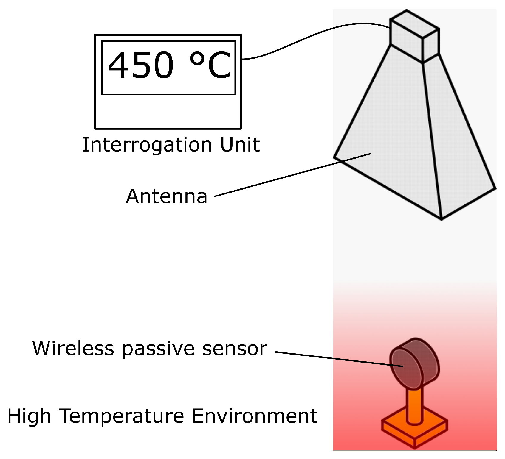
Sensors are essential components of any control system. For many applications, the size of the sensor matters; for ubiquitous sensing, the financial and environmental costs per sensor must be minimized. In aerospace, automotive, or process control industries, sensors often have to be installed in harsh environments. Wireless sensors, called transponders, are used in moving or rotating control points, on or in living beings, in harsh conditions, and where wiring would be expensive. Chipless passive transponders enable measurements without integrated circuits, wiring, or battery installation at the measuring point, thus increasing the robustness, functionality, and lifetime of the system under test. Such a transponder system consists of two parts: (i) a reader; (ii) passive transponders that act as cooperative targets. Both parts are connected via a wireless connection, usually a radio link, as shown in Figure 1.

Three types of chipless passive transponders are presented in the literature: delay lines, resonators, and mixers [1]. This article focuses on transponders made of dielectric resonators with a high overall quality factor Q (see Appendix A), where temperature changes the resonator’s resonance frequency. To excite the passive transponder, the reader sends a read signal to the transponder via a radio channel. This signal is received there and excites an oscillation in the resonator. After the read signal is switched off, the oscillation decays exponentially. Part of the energy stored in the oscillation is sent back to the reader as a backscattered signal, where it is received, sampled, and evaluated. The resonance frequency can be extracted if the oscillation’s decay time is long enough to separate it from the read signal and all larger ambient echoes of the radio channel. To achieve high resolution with a large reading range, the overall quality factor Q must be in the range of several hundred to several thousand [2].

Due to the low complexity of chip-less passive transponders and the operation without any battery or electronic circuity, the instrumentation technique is considered to be maintenance-free, robust, and can be operated in harsh environments. Systems with chipless passive transponders usually outperform radio frequency identification (RF-ID)-based transponder systems in terms of both temperature load and reading distance. Their maximum operating temperature is limited only by the assembly technology and the temperature resistance of the conduction lines. Since they are linear time-invariant systems, their reading distance is only limited by receiver noise, which blocks the detection of a response signal from distances beyond the maximum reading distance.

Contemporary passive wireless temperature sensors are often based on surface acoustic wave (SAW) devices [1,3]. However, their size is not determined by the small SAW chip but by the bulky antenna. They have shown a reliable operating range up to 350 °C and, in exceptional cases, even significantly higher [4]. A dielectric resonator could enable a simpler, smaller, and more heat-resistant chipless passive transponder.

Dielectric resonators have been used in microwave-integrated circuits, antenna systems, and communication applications for many years. They were discovered in 1939 when it was shown that non-metallic dielectric objects are similar to metal cavities in their ability to confine electromagnetic fields [5,6]. However, due to high material dielectric loss and low temperature stability, dielectric resonators were rarely applied for several decades [7]. This changed in the 1980s when new ceramic technology provided low-loss and temperature-stable materials for dielectric resonators [8,9,10]. An example of such a highly stable ceramic, zirconium tin titanate, $(Zr-Sn)Ti{O}_4$, is used in this study.

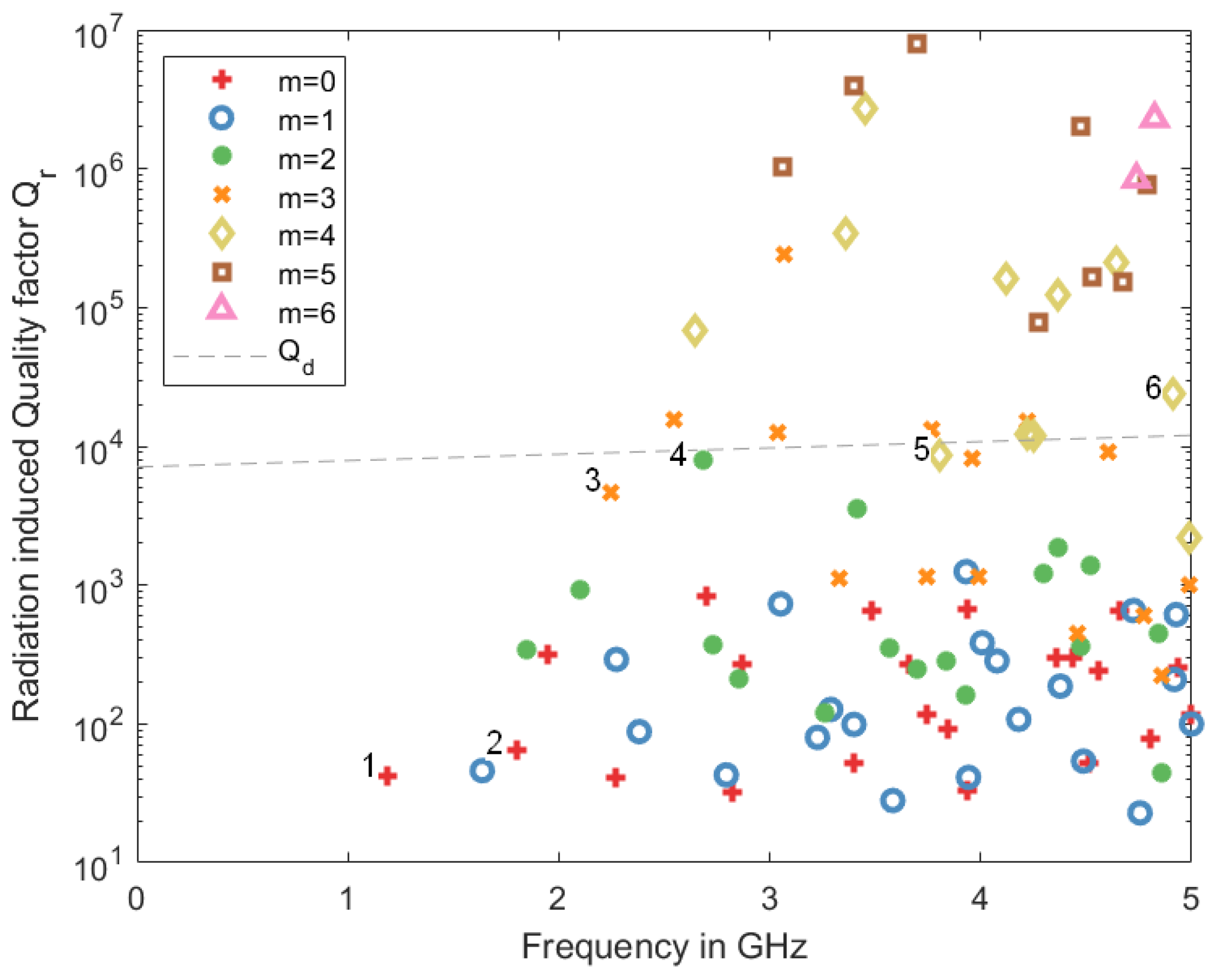
The use of a dielectric resonator as a sensor allows the combination of the functions of a resonator and an antenna in a single element. The dielectric resonator does not completely encapsulate the standing electromagnetic wave but rather exhibits low leakage. The overall quality factor Q is thus determined by two factors (see Appendix A): the dissipative and the radiation-induced Q-factor. To maximize the signal-to-noise ratio, the radiation-induced Q-factor should be similar to the dissipative Q-factor, and both should be high [2].

The transponder then consists of just one single small element that functions as both a resonator and antenna. This not only makes the transponder unbeatably small but also greatly increases its robustness against mechanical and thermal stress. Since the resonator also acts as an antenna, it is sensitive to conductive materials in its environment.

Ceramic dielectric resonators have been presented in the scientific literature for measuring temperature [11,12,13,14,15,16,17]; however, most applications include some metallic housings and additional antennas. The use of a bare-die dielectric resonator as a wireless passive chipless transponder is rare [18,19,20,21,22]. This work continues the work reported in [18] and extends it both simulatively and experimentally.

Due to its availability as unpacked dielectric resonators from the development of base station filters, its relatively high dielectric constant of ${ϵ}_r=37$, and its high temperature resistance, a dielectric resonator made of zirconium tin titanate (ZST) was chosen for this study. 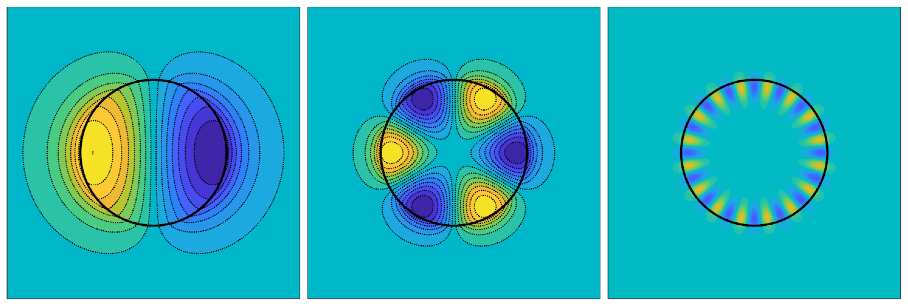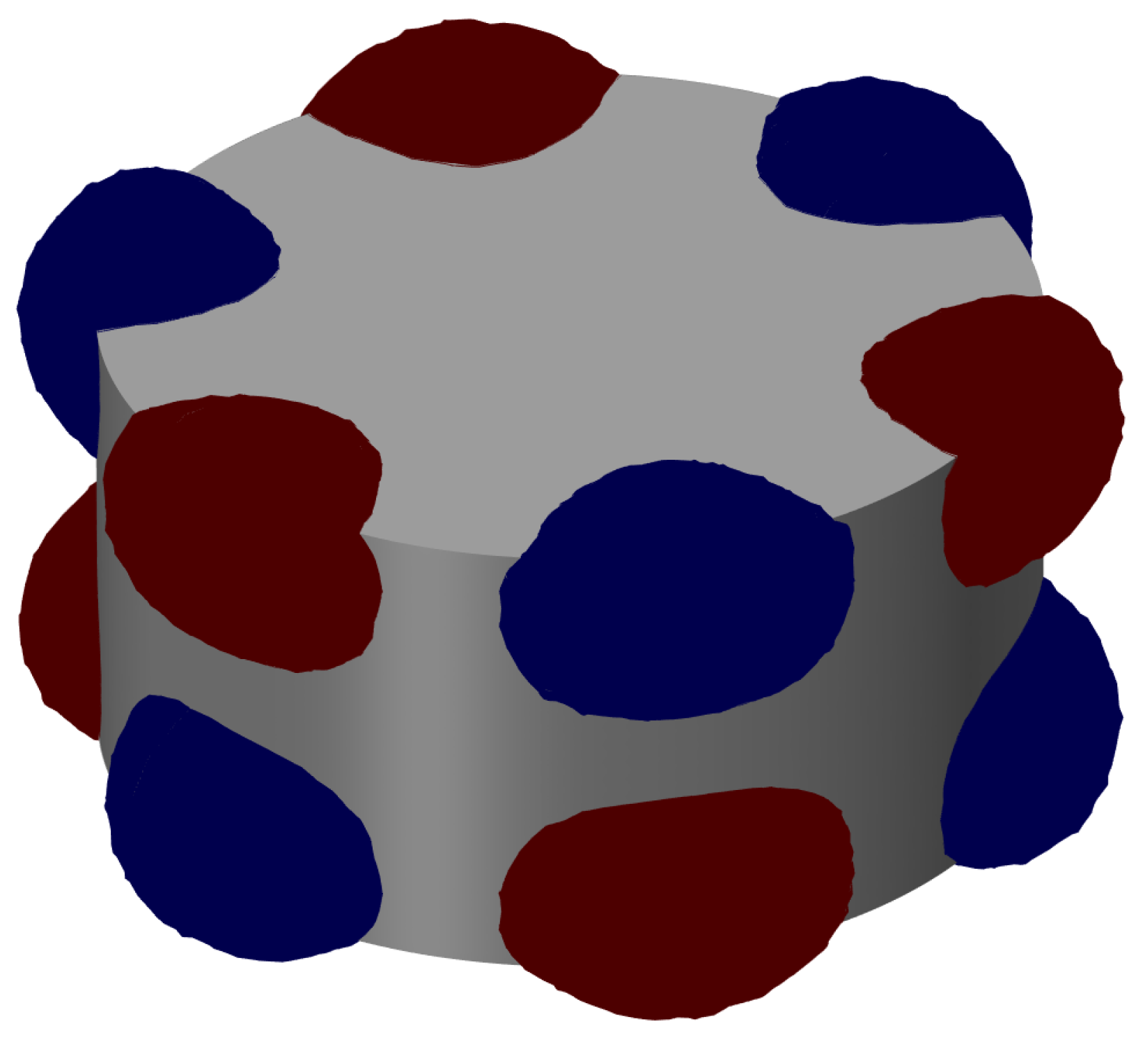The dielectric resonator is modeled using the finite element method (FEM) in the commercial program COMSOL 5.2 Multiphysics^® [23]. The fundamental mode radiates very strongly electromagnetically and, thus, features a low overall Q-factor. However, some higher modes, such as the $HE{M}_{31\delta }$ mode, combine a good balance between radiative coupling and energy storage within the resonator and are, therefore, ideally suited for use as a passive chipless transponder.

For an experimental verification of the simulations, we placed isolated dielectric resonators with high radiation Q-factors on a low-loss, low permittivity ceramic holder and measured their radiation properties in the far field. The radiation patterns investigated in the laboratory and outdoors agree well with the simulations. The resulting radiation patterns show a directivity of approximately 7.5 dBi at 2.5 GHz. The sensor was then heated in a ceramic furnace. The readout antenna was located outside at room temperature. Wireless temperature measurements up to 700 °C, with a resolution of 0.5 °C, experimentally prove the outstanding performance of dielectric resonators for practical applications.

2. Design of Dielectric Passive Transponder

2.1. Isolated Dielectric Resonator

To design and analyze a dielectric passive resonator for a one-piece passive transponder application, we performed an electromagnetic simulation. The geometry of the dielectric resonator is assumed to be a flat cylindrical disk comparable to a puck in ice hockey. This results in the geometric constant radius, height, and dielectric constant of the medium. Characteristic quantities for the resulting modes are resonance frequency, quality factor, and a metric for radiation coupling—the radiation-induced Q-factor.

To calculate the resonance frequencies and quality of the different eigenmodes of a dielectric resonator, either an analytical eigenvalue problem can be solved as outlined in the book by Kajfez and Guillon [24] or a commercial solver for electromagnetic problems can be used. In this manuscript, approximations to Maxwell’s equations are used for a numerical calculation of the resonance frequencies, the dissipative, and the radiation-induced Q-factors.

To simulate the electromagnetic properties, a layout of the geometry is first designed on the computer. In addition, the electrical and magnetic properties of the materials used must be determined. For the electromagnetic code, the desired geometry is then approximated by a mesh model. The mesh density is determined from geometric features and the operating frequency. The initial condition is that the edge lengths of each element at the operating frequency do not exceed one-tenth of a wavelength. As the frequency increases, the number of elements in the mesh therefore increases [25]. After completing a simulation, it is repeated with a slightly different mesh density to test whether the simulation results converge, i.e., are independent of the chosen discretization. If this is not the case, the mesh is refined until convergence is achieved [25].

COMSOL Multiphysics enables a 2D approximation of axisymmetric three-dimensional electromagnetic problems. A cylindrical dielectric resonator floating in free space is thereby investigated in a 2.5D axisymmetric simulation. An example setup of this simulation is shown in Figure 2. A high permittivity cylindrical dielectric resonator is surrounded by a sphere of air encapsulated in a perfectly matched layer (PML) from all sides. An axis of symmetry bounds the two-dimensional space from the left side. We used a triangular mesh for the resonator and the surrounding medium, but a regular rectangular mesh was used for the perfectly matched layer. This is performed to improve the numerical stability of the perfectly matched layer and to suppress spurious reflections coming back from it.

Before starting the calculations, an azimuthal mode number m is specified, a non-negative integer that characterizes the periodicity of the fields around the axis of symmetry. To study the radiation-induced Q-factor of the fundamental $T{E}_{01\delta }$ mode, a resonator at 2.5 GHz is designed for a varying dielectric constant. For this investigation, we varied the relative permittivity in the range of $ϵ$ = 100–300. This roughly corresponds to the range of the dielectric constant of Strontium Titanate [26].

Figure 3 shows that the size (diameter and thickness) of the resonator decreases with the relative permittivity, as expected. It also shows that the radiation-induced Q-factor increases as a larger fraction of the electrical field is enclosed in the dielectric pill, thus the total electromagnetic radiation decreases. However, the increase in the radiation-induced Q-factor as a function of permittivity is not nearly high enough, using realistic materials, for an application of the $T{E}_{01\delta }$ mode in a wireless dielectric transponder. Therefore, we investigated higher modes with higher radiation-induced Q-factors and/or metallic housings that enable effective radiation.

2.2. Higher Order Modes of the Isolated Dielectric Resonator

We performed the same numerical studies with the setup shown in Figure 2, but for higher order modes. The results from these simulations are summarized in Figure 4.

Figure 4 depicts the resonance frequencies and the radiation-induced Q-factors of the first 34 modes. The dielectric material is chosen to be Zirconium Tin Titanate (${ϵ}_r$ = 37). The dielectric resonator has a cylindrical shape with a diameter of 40 mm and a thickness of 20 mm. The modes are labeled according to the convention described in [24], with TM being a transverse magnetic mode and HEM a hybrid electromagnetic mode.

In the simulation, the value for the dielectric dissipation factor ($tan\left(\mathrm{\delta }\right)$) is set to ‘0’, which makes the simulated loaded Q-factor equal to the radiation-induced Q-factor. The dissipative-induced Q-factor with Zirconium Tin Titanate is shown in Figure 4 with a black dashed line.

Many modes exhibit radiation-induced Q factors on the order of a few hundred or less. The resulting total Q factors of these modes appear to be too low for use in a wireless sensor system, as the resonator would decay before the ambient echoes decay. Figure 5 shows on the left the magnetic field component in the z-axis of one of these modes, $HE{M}_{11\delta }$.

On the other hand, we observe resonances with very high radiation Q-factors above ${10}^5$. At these resonances, the attenuation by electromagnetic radiation is significantly lower than the dissipative attenuation in the dielectric, making them very unsuitable for passive wireless chipless transponders. Figure 5 shows on the right the magnetic field component in the z-axis of one of these modes, $HE{M}_{16,1(\delta +1)}$.

Near the line for dissipatively induced Q-factor of zirconium tin titanate, we find hybrid electromagnetic modes with azimuthal mode numbers 3 or 4, for example, $HE{M}_{31(\delta +1)}$, which are damped by electromagnetic radiation to a similar extent as by dissipative material losses. Since the overall decay constant of these modes is sufficiently long compared to typical ambient echoes of the radio channel, they are well suited for wireless readout applications. These modes have the unique property that a single dielectric resonator acts as both a resonator and an antenna. Figure 5 shows in the center the magnetic field component in the z-axis of the mode $HE{M}_{31(\delta +1)}$.

The $HE{M}_{31(\delta +1)}$ mode is further investigated in the experimental setup discussed in Section 4, where also a comparison is performed between the simulated resonant frequency and quality factors for three of the most prominent modes in Zone 2.

The horizontal radiation pattern in Figure 6 on the left side also shows the six-fold symmetry of the electrical fields in the far field that is observed in the center graph of Figure 5. The radiation pattern on the right side of Figure 6 depicts the far-field electric field strength as a function of elevation in polar coordinates. This is a cross-section of the radiating lobe in the vertical plane. The vertical radiation pattern appears identical to a dipole, whereas the horizontal shows a six-fold symmetry. The magnitude of the electric fields as a function of space is also shown in Figure 6 in the rightmost sub-figure. The fields resulting from an eigenmode solution of FEM equations look very identical to the analytically calculated fields shown in Figure 5; this allows us to identify the mode as the $HE{M}_{31(\delta +1)}$ mode of an isolated dielectric resonator.

For an isolated dielectric resonator, operating in the $HE{M}_{31(\delta +1)}$ mode, iso-surfaces for constant values of positive and negative H-field z-component are displayed in Figure 7 as red and blue solids. The dielectric resonator is represented as a gray cylinder. The shape of the field suggests that six dipoles are equidistantly arranged around the circumference with alternating polarities.

Since the resonator has circular symmetry, rotating the resonator does not change the radiation pattern. To measure the horizontal radiation pattern, a bistatic setup would be required in which the receiving antenna is rotated around the axis of symmetry. The vertical polarization of the radiation of the dielectric resonator, however, can be measured quite simply by rotating its vertical axis and recording the amplitude of the decaying eigenmode as a function of the angle of rotation. This measurement will be presented in Section 3.

2.3. Sectioned Cylindrical Dielectric Transponder

An increase in directivity, along with a reduction in the size of the antenna, can be achieved by restricting the radiation pattern to one lobe. This can be realized by using two metal plates, which are inserted at the symmetry planes, and using the mirror charges on the conductor to complement the fields in the main lobe. Figure 8 shows the setup of a 60° section of a dielectric resonator bounded by perfectly conducting finite sheets of metal.

According to the far-field simulation results in Figure 8, the directivity can be increased by a factor of 6; however, the gain is not increased by a factor of 6 due to the conductivity losses in the metal plates. The optimization of this focusing beam resonator retro-reflector is left over for future investigation.

3. Measurement of the Electromagnetic Radiation Pattern of a Dielectric Resonator

To verify the vertical radiation pattern of the dielectric resonator calculated in Section 2.2, the experimental setup shown in Figure 9 was chosen. A dual-polarized, high-gain broadband horn antenna [27] with a frequency range of 0.7–7 GHz and a maximum gain of 15 dBi is installed horizontally on an antenna holder. In the beam of the antenna, an isolated dielectric resonator is placed on the edge of a low-loss, low permittivity ceramic holder, which is mounted on top of an electronically controlled turntable. The axis of rotation of the turntable is parallel to the vertical polarization and perpendicular to the axis of symmetry of the dielectric resonator.

A motion controller with an optical encoder for feedback is implemented and connected via RS-232 to a data acquisition and control computer running a LabView program. An Agilent 5071B network analyzer (NWA) is also connected via the IEEE bus to the computer. The setup is controlled by a finite state machine with two main states: (1) rotate the turntable; (2) trigger the NWA measurement. The transition from state 1 to 2 will start when zero angular velocity is measured by the optical encoder, and the transition from state 2 to 1 is made when the measurement data transfer to the program is complete. We carried out a 1–5 GHz 2 port measurement with a frequency step of 50 kHz and an IF bandwidth of 15 kHz for each angle and both polarizations of the horn antenna. Additional cross-polarization data were also collected in the S21 and S12 columns. In order to suppress reflections from the environment, all the measurements were performed outdoors in a grass field, and the high-gain antenna suppressed possible ground reflections. In the post-processing algorithm, the resonance peaks were isolated and gated in the time domain to remove further environmental effects.

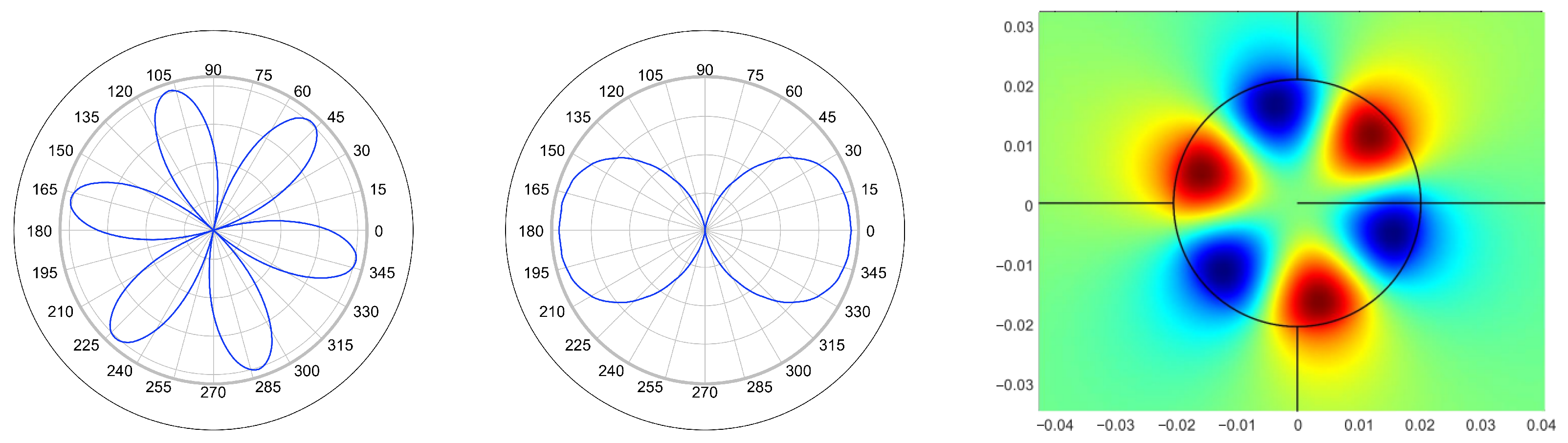
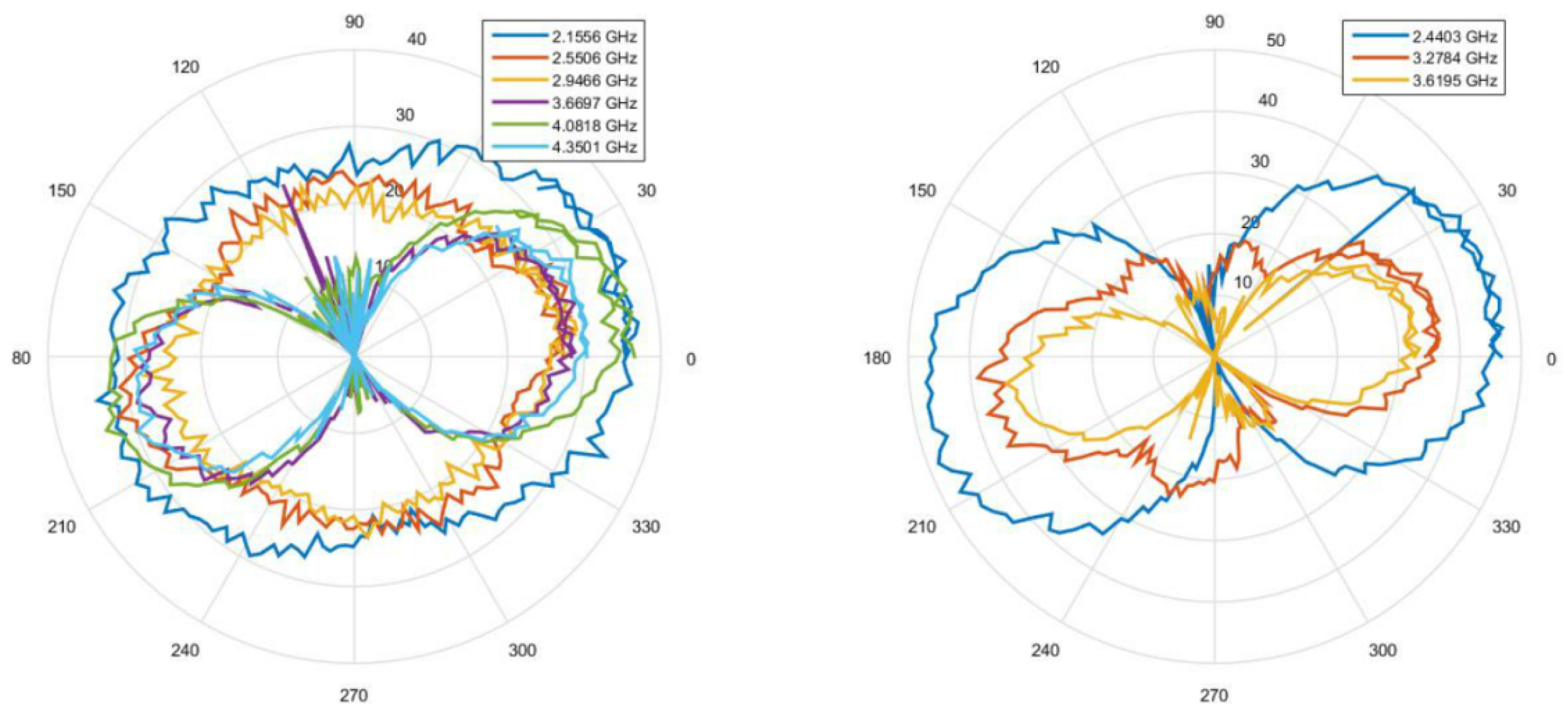
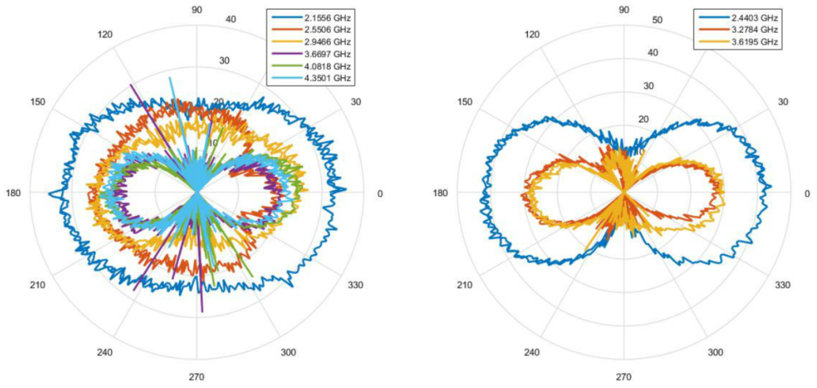
The amplitude of the resonance signal of the $HE{M}_{31(\delta +1)}$ as a function of the turntable angle is shown in Figure 10 and Figure 11. Figure 10 shows the modes of the resonator that were excited and detected by the vertically polarized radiation of the horn antenna, and Figure 11 shows the modes that were excited and detected by the horizontally polarized radiation of the horn antenna.

The center graph of Figure 6 depicts the calculated radiation pattern of the $HE{M}_{31(\delta +1)}$ mode, which rings at 2.4403 GHz for the dimensions of the resonator under test. The corresponding measured radiation pattern is shown in blue color in the right graphs of Figure 10 and Figure 11. Other modes of different orders also have dipole characteristics.

In the measurements, we observed that low-order dipoles exhibit a low radiation Q-factor. This phenomenon is in good agreement with the simulation results in Section 2.2 as, due to field confinement, an increase in the radiation Q-factor for higher order modes is also observed numerically. The far-field radiation pattern will exhibit the same symmetry as the field pattern of the resonance modes.

The resonator operating on the $HE{M}_{31(\delta +1)}$ mode is used as wireless passive transponder for high temperature measurements in the next section.

4. High Temperature Measurements

The resonator operating on the $HE{M}_{31(\delta +1)}$ combines both functionalities; it provides a high Q-factor of oscillation with dielectric losses nearly equal to radiation losses, and it couples well with free space electromagnetic radiation, eliminating the need for any additional antenna. No conductive boundary to encapsulate the electromagnetic fields of the resonator is needed. This allows for an extremely high temperature load on the transponder and keeps the high overall Q-factors even at elevated temperatures of more than 500 °C.

Figure 12 illustrates the schematic setup of a wireless high temperature measurement experiment. A high-gain antenna is installed outside the high temperature area and aligned with a dielectric resonator sensor. Radiation from one or more of the HEM modes shown in the simulation results in Figure 5 couple to the antenna via electromagnetic waves. As described in Figure 1, a reader detects the resonant frequency and compares it with a pre-calibrated lookup table defined by a second-order polynomial to calculate the temperature at the sensor. The experimental setup for such a high temperature wireless measurement is shown in Figure 13. The dielectric resonator is placed on a low permittivity dielectric holder within a high temperature oven. The sides of the oven are metallic and the top and bottom are a low permittivity ceramic material, thus top and bottom of the over are transparent to EM microwaves.

A PID controller with a PT-100 reference element is used to control the temperature in the oven and, thus, the temperature on the dielectric resonator. The PID controller is connected via RS-232 to the data acquisition and control computer running a LabView program. The dual-polarized horn antenna is connected to two ports of the Agilent 5071B NWA, which is also connected to the laptop via the IEEE bus. The PID controller is programmed with a linear temperature ramp from room temperature to 700 °C over a duration of 15 h. The LabView program regularly collects the current temperature from the PT100 element and measurement data from the NWA and stores it with a time stamp.

The multi-mode resonator is irradiated by radio waves generated from an NWA that is used as a stepped frequency continuous wave radar. From the frequency domain sampling, all multiple resonant frequencies can be extracted. A Short Time Fourier Transform is performed on the zero-padded frequency domain data, and a spectrogram is produced as depicted in the left graph of Figure 14. Every resonance produces a long reverberation and, thus, a long tail in the time domain. The higher the overall Q-factor, the longer the reverberation.

To separate the individual resonant frequency bands shown in the right-hand graph, the time domain from 0 to 300 ns is gated out, and the remaining signal components are transformed into the frequency domain. Three dominant modes with different overall Q-factors and different radiation couplings between the dielectric resonator and the antenna emerge. The noise floor of the measurement is −105 dB, and the strongest peak features a signal-to-noise ratio of 40 dB at a distance of over 50 cm between the antenna and the resonator and with the radio waves attenuated twice by the ceramic cover.

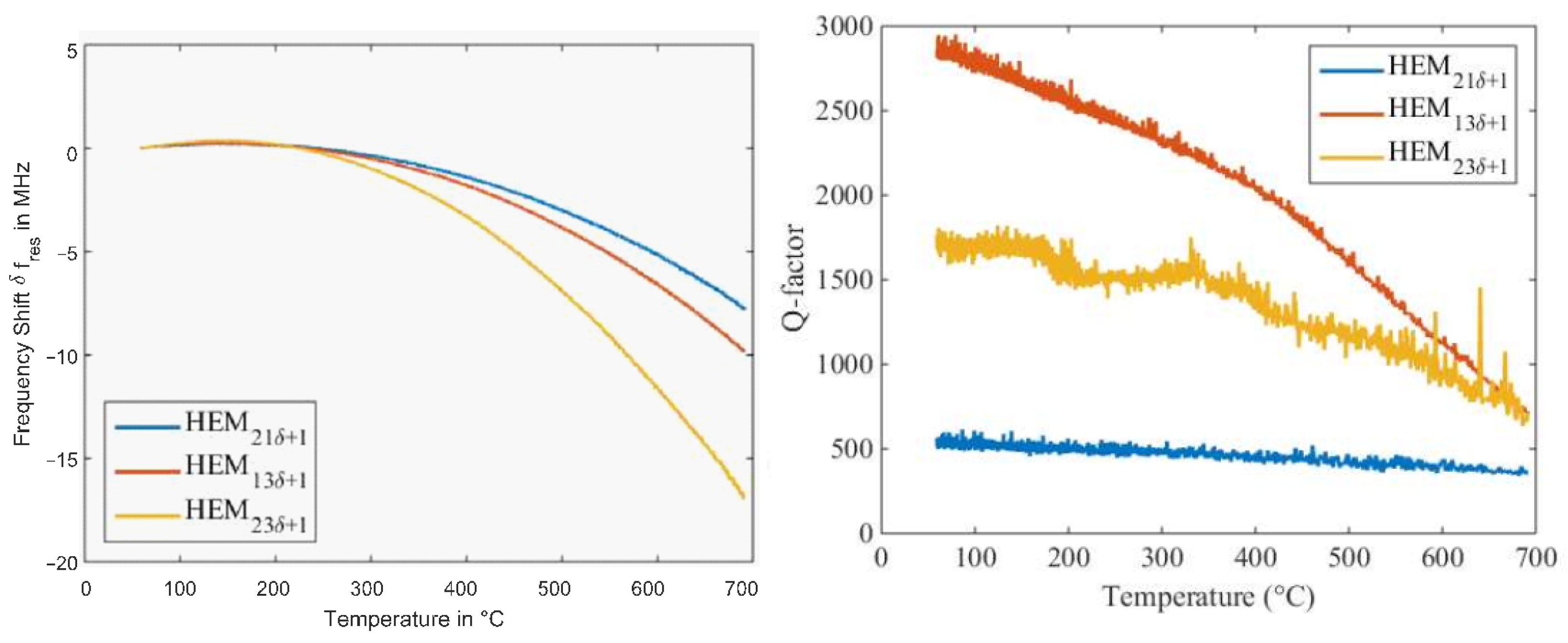
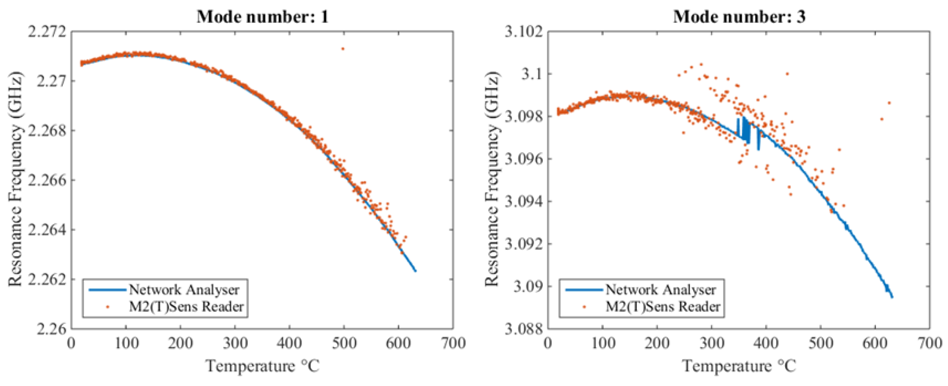
The frequencies of the three resonances shown in Figure 14 were then monitored as a function of temperature. Figure 15 shows their frequency shift and Q-factor variation as a function of temperature. The inflection points of the temperature sensitivity for the material used here lie between room temperature and 200 °C. The three modes exhibit three different negative square temperature coefficients of the resonance frequency, which can be used for more precise temperature determination.

The overall Q factor shows a monotonically decreasing function of temperature due to increasing dielectric losses in the materials. Increasing losses at high temperatures in the radio channel of the experimental setup might also contribute to the lowered Q factor: The radio waves pass through the fire clay of the oven, which has a small but non-negligible electrical conductivity at high temperatures, resulting in an increase in absorption of the radio waves two times for a single measurement. In addition, the ceramic holder on which the resonator is located can also exhibit increased conductivity and, thus, increased damping at higher temperatures.

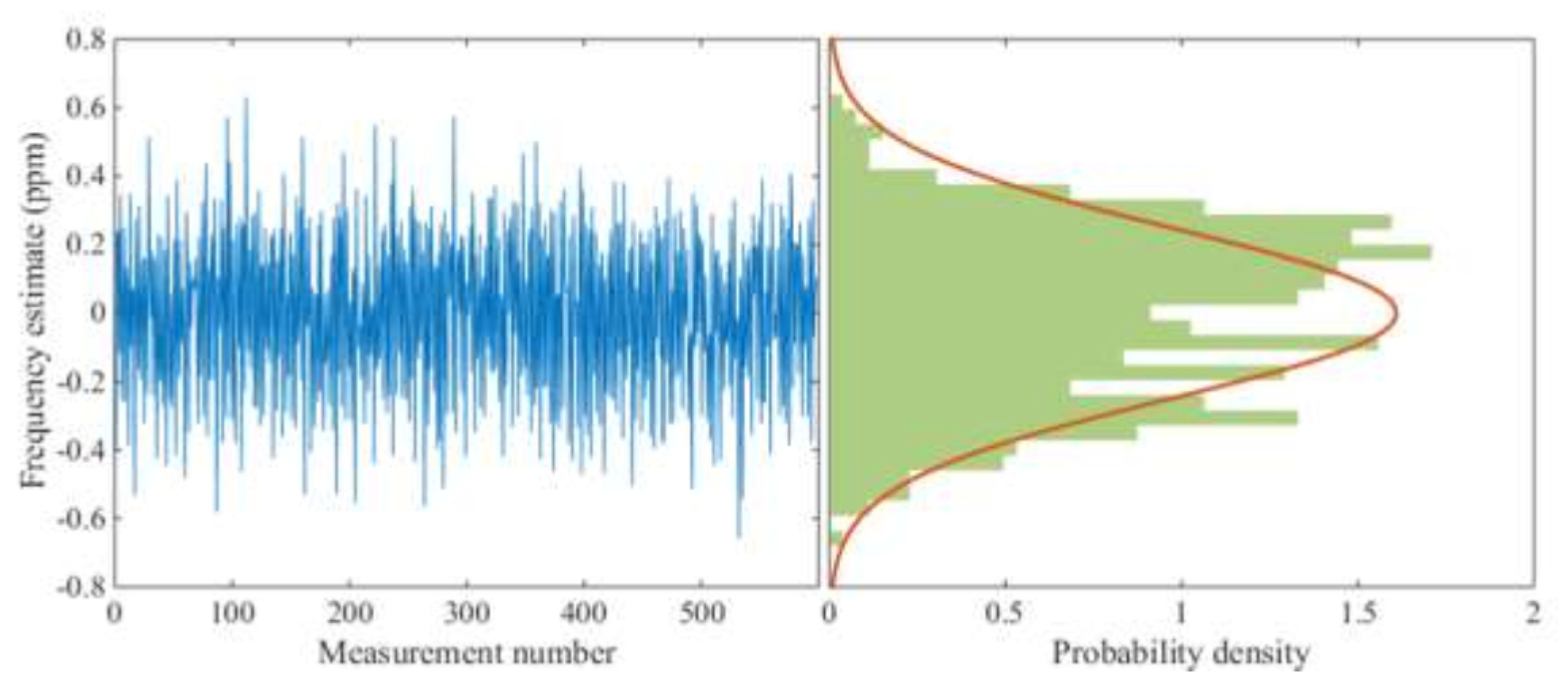
Figure 16 shows the variance of the resonance frequency of a mode for 600 consecutive measurements. The sensor is placed in the high temperature furnace, and the temperature is fixed at 500 °C. Slight fluctuations in the center frequency due to the furnace temperature control are visible in the time series. To compensate for these tiny deviations, a non-contact measurement of the actual temperature of the resonator with an accuracy of better than 0.1 °C at 500 °C would have been necessary, but this was beyond the capabilities of the laboratory.

On the right-hand side of Figure 16, a histogram and an approximated Gaussian distribution are created from these data, resulting in a 1 $\sigma$ standard deviation, which corresponds to a temperature uncertainty of 0.5 °C. This uncertainty can be reduced by filtering or averaging the raw signal. The actual uncertainty of temperature measurement with a dielectric resonator could be below 0.5 °C since the uncertainty shown in Figure 16 is caused by the joint contributions of the furnace temperature control and the measurement accuracy. Furthermore, a sub-optimal parabolic fit was used to evaluate the resonance frequency [2]. The authors assume that due to the influence of the furnace control loop, the distribution of the frequency deviations does not exactly follow a Gaussian distribution and, moreover, shows an asymmetric distribution of the frequency deviations.

A simple tracking algorithm might run into problems if two modes are very close in the frequency domain or if two crossing modes are tracked. Such a possible tracking failure is shown in Figure 17. The simple tracking algorithm jumps between both modes depending on signal strength. This problem might be overcome by more advanced algorithms in the future.

5. Summary and Conclusions

This manuscript presents a theoretical and experimental study on the use of bare-die dielectric resonators as wireless, passive temperature sensors, which do not require integrated circuits, batteries, or antennas because the electromagnetic fields in the dielectric resonators are coupled to free-space electromagnetic waves. A resonator itself acts as an analog storage for the read signals, as a sensor, and as an antenna. For the fundamental mode and several higher modes of an isolated dielectric resonator based on Zirconium Tin Titanate (ZST, ${ϵ}_r$ = 37), the resonance frequencies, quality factors, and couplings to electromagnetic waves were calculated using a finite element method in COMSOL Multiphysics. For the fundamental mode, the coupling to the far-field electromagnetic wave is so strong that the overall Q factor remains below 100, which is too low for a wireless passive sensor. Some higher modes, such as the $HE{M}_{31\delta }$ mode, have a radiation Q factor, about half of the overall Q factor, which makes them ideal as wireless passive sensors.

To characterize the dielectric resonators, several experiments were conducted in which they were placed on a dielectric holder. The vertical radiation patterns of some higher modes agreed well with the simulation results, showing total Q factors of up to 3000 and a directivity of approximately 7.6 dBi at 2.44 GHz. For temperature measurements, the sensor was placed in a ceramic furnace, and the reading antenna was placed outdoors at room temperature. Wireless temperature measurements up to 700 °C were demonstrated with a resolution of 0.5 °C from a distance of 1 m.

Future research could investigate other well-suited or even better-suited materials, such as strontium titanate, for their suitability for high temperature measurement technology based on dielectric resonators. Material optimizations with regard to higher temperature tolerance, higher dielectric constant for size reduction, and higher quality factors in combination with reduced conductivity losses at high temperatures could also significantly advance the technology.

Radiating dielectric resonators act as small antennas. Conductive or magnetizable materials in the range of approximately two wavelengths change their radiation properties and also pull the resonant frequency. In a static setup with conductive or magnetizable materials, wireless measurement of the resonator temperature or temperature change is still feasible. In a dynamic setup, however, some components of the evanescent field must be shielded. This leads to additional conduction losses, especially at high temperatures.

References

1. Reindl, L.; Scholl, G.; Ostertag, T.; Scherr, H.; Wolff, U.; Schmidt, F. Theory and application of passive saw radio transponders as sensors. IEEE Trans. Ultrason. Ferroelectr. Freq. Control 1998, 45, 1281–1292. [Google Scholar] [CrossRef] [PubMed]
2. Reindl, L.M.; Aftab, T.; Schaechtle, T.; Ostertag, T.; Luo, W.; Rupitsch, S.J. Estimation of the Measurement Accuracy of Wireless Passive Resonance Sensors. Sensors 2025, 25, 747. [Google Scholar] [CrossRef] [PubMed]
3. Bao, X.Q.; Burfhand, W.; Varadan, V.V.; Varadan, V.K. SAW temperature sensor and remote reading system. In Proceedings of the IEEE Ultrasonics Symposium, Denver, CO, USA, 14–16 October 1987; pp. 583–585. [Google Scholar]
4. Davulis, P.M.; Da Cunha, M.P. High-temperature langatate elastic constants and experimental validation up to 900 °C. IEEE Trans. Ultrason. Ferroelectr. Freq. Control 2010, 57, 59–65. [Google Scholar] [CrossRef] [PubMed]
5. Richtmyer, R.D. Dielectric resonators. J. Appl. Phys. 1939, 10, 391–398. [Google Scholar] [CrossRef]
6. Okaya, A.; Barash, L.F. The Dielectric Microwave Resonator. Proc. IRE 1962, 50, 2081–2092. [Google Scholar] [CrossRef]
7. Wang, C.; Zaki, K.A. Dielectric resonators and filters. IEEE Microw. Mag. 2007, 8, 115–127. [Google Scholar] [CrossRef]
8. Fiedziuszko, S.J.; Holmes, S. Dielectric resonators raise your high-Q. IEEE Microw. Mag. 2001, 2, 50–60. [Google Scholar] [CrossRef]
9. Fiedziuszko, S.J.; Hunter, I.C.; Itoh, T.; Kobayashi, Y.; Nishikawa, T.; Stitzer, S.N.; Wakino, K. Dielectric materials, devices, and circuits. IEEE Trans. MTT 2002, 50, 706–720. [Google Scholar] [CrossRef]
10. Ren, X.; Jiang, T.; Wang, Y.; An, L.; Gong, X. Characterization of high-temperature ceramic materials at microwave frequencies for MEMS applications. In Proceedings of the 2009 IEEE 10th Annual Wireless and Microwave Technology Conference, Clearwater, FL, USA, 20–21 April 2009; pp. 1–4. [Google Scholar] [CrossRef]
11. Kenji, I. Remote Measuring Thermometer. Patent JP000S60203828A, 15 October 1985. Available online: https://depatisnet.dpma.de/DepatisNet/depatisnet?action=pdf&docid=JP000S60203828A&xxxfull=1 (accessed on 14 February 2024).
12. Takeshi, O. Non-Contact Temperature//Pressure Detection Method by Ultrasonic Wave. Patent JP000H01119729A, 11 May 1989. Available online: https://depatisnet.dpma.de/DepatisNet/depatisnet?action=pdf&docid=JP000H01119729A&xxxfull=1 (accessed on 14 February 2024).
13. Ostertag, T.; Reindl, L.; Ruile, W.; Scholl, G. Sensor System. Patent EP 677752, 27 June 2001. Available online: https://depatisnet.dpma.de/DepatisNet/depatisnet?action=pdf&docid=EP000000677752B1&xxxfull=1 (accessed on 14 February 2024).
14. Ren, X.; Gong, X. A wireless sensing technique using passive microwave resonators. In Proceedings of the 2008 IEEE Antennas and Propagation Society International Symposium, San Diego, CA, USA, 5–11 July 2008; pp. 1–4. [Google Scholar] [CrossRef]
15. Cheng, H.; Ren, X.; Ebadi, S.; Chen, Y.; An, L.; Gong, X. Wireless Passive Temperature Sensors Using Integrated Cylindrical Resonator/Antenna for Harsh-Environment Applications. IEEE Sens. J. 2015, 15, 1453–1462. [Google Scholar] [CrossRef]
16. Schueler, M.; Mandel, C.; Puentes, M.; Jakoby, R. Metamaterial inspired microwave sensors. IEEE Microw. Mag. 2012, 13, 57–68. [Google Scholar] [CrossRef]
17. Gu, T.; Wang, B. Design of a Metamaterial Chipless RFID Sensor Tag for High Temperature. In Proceedings of the 2022 International Conference on Frontiers of Communications, Information System and Data Science (CISDS), Guangzhou, China, 25–27 November 2022; pp. 160–164. [Google Scholar] [CrossRef]
18. Boccard, J.-M.; Aftab, T.; Hoppe, J.; Yousaf, A.; Hütter, R.; Reindl, L.M. High-Resolution, far-field, and passive temperature sensing up to 700 °C using an isolated ZST microwave dielectric resonator. IEEE Sens. J. 2016, 16, 715–722. [Google Scholar] [CrossRef]
19. Corbellini, S.; Ramella, C.; Yu, L.; Pirola, M.; Fernicola, V. Whispering Gallery Mode Thermometry. Sensors 2016, 16, 1814. [Google Scholar] [CrossRef] [PubMed]
20. Jiménez-Sáez, A.; Schumacher, P.; Häuser, K.; Schüßler, M.; Binder, J.R.; Jakoby, R. Chipless Wireless High Temperature Sensing Based on a Multilayer Dielectric Resonator. In Proceedings of the 2019 IEEE SENSORS, Montreal, QC, Canada, 27–30 October 2019; pp. 1–4. [Google Scholar]
21. Wang, Q.; Liu, Y.; Zhang, M.; Bai, X.; Gao, Z. A simple dielectric resonator-based sensor for temperature measurement. Results Phys. 2021, 27, 104481. [Google Scholar] [CrossRef]
22. Xiong, J.; Wu, G.; Tan, Q.; Wei, T.; Wu, D.; Shen, S.; Dong, H.; Zhang, W. Dielectrically-Loaded Cylindrical Resonator-Based Wireless Passive High-Temperature Sensor. Sensors 2016, 16, 2037. [Google Scholar] [CrossRef] [PubMed]
23. COMSOL 5.2 Multiphysics®; COMSOL AB: Stockholm, Sweden, 2014; Available online: www.comsol.com (accessed on 20 May 2025).
24. Kajfez, D.; Guillon, P. Dielectric Resonators, 2nd ed.; SciTech Publishing: Atlanta, GA, USA, 1998. [Google Scholar]
25. Niziolek, M. Review of methods used for computational electromagnetics. In Proceedings of the 2nd International Students Conference on Electrodynamic and Mechatronics, SCE 11 ’09, Opole, Poland, 19–21 May 2009; pp. 15–16. [Google Scholar]
26. Neville, R.C.; Hoeneisen, B.; Mead, C.A. Permittivity of Strontium Titanate. J. Appl. Phys. 1972, 43, 2124–2131. [Google Scholar] [CrossRef]
27. Antenna BBHX 9120 E from SCHWARZBECK MESS—ELEKTRONIK OHG. Available online: https://schwarzbeck.de/en/antennas/broadband-horn-antennas/double-ridged-horn-antenna.html (accessed on 20 May 2025).
28. Kobayashi, Y.; Aoki, T.; Kabe, Y. Influence of conductor shields on the Q-factors of a TE0 dielectric resonator. IEEE Trans. Microw. Theory Tech. 1985, 33, 1361–1366. [Google Scholar] [CrossRef]
Figure 1. Schematic of the operation of a transponder system using passive resonant sensors: A reader sends a read signal to the sensor node over a radio channel. This signal is received there and stored in an oscillation in the resonator. When the read signal is switched off, the resonator will oscillate with an exponentially decreasing amplitude at a frequency modified by the quantity to be measured, in this case, the temperature. A part of the stored energy is sent back to the reader as a backscatter signal. There, it is received, sampled, and evaluated.
Jsan 14 00060 g001
Figure 2. A 2D axis-symmetric and a 3D mesh for a FEM simulation in COMSOL.
Jsan 14 00060 g002
Figure 3. Size and radiation-induced Q-factor for an isolated dielectric transponder resonating at 2.5 GHz on the T E 01 δ mode as a function of the dielectric constant.
Jsan 14 00060 g003
Figure 4. Overview of FEM simulation results where the radiation-induced Q-factor is plotted as a function of resonant frequency for the first 34 modes. The modes are labeled according to [24], where TM describes a transverse magnetic mode and HEM a so-called hybrid electromagnetic mode. The labeled modes are as follows: 1: T E 01 δ ; 2: T M 01 δ ; 3: H E M 31 ( δ + 1 ) ; 4: H E M 22 ( δ + 1 ) ; 5: H E M 42 ( δ + 1 ) ; 6: H E M 42 ( δ + 3 ) .
Jsan 14 00060 g004
Figure 5. Magnetic field components in the z-axis of some radiating HEM modes of the dielectric resonator, left the H E M 11 δ , center the H E M 31 ( δ + 1 ) , and right the H E M 16 , 1 ( δ + 1 ) mode.
Jsan 14 00060 g005
Figure 6. Horizontal (left) and vertical (center) far-field radiation pattern as absorbed by the perfectly matched layer for the H E M 31 ( δ + 1 ) mode. The figure on the right shows the field patterns with circular symmetry, which was generated by the 3D-FEM solver.
Jsan 14 00060 g006
Figure 7. Three dimentional iso-surface plot of the z-component of the H-field. Here, the positive fields are in blue and the negative ones in red. The six dipoles can be seen distributed along the circumference of the dielectric resonator.
Jsan 14 00060 g007
Figure 8. Setup (left), calculated electrical field intensity (center) and far-field electrical field strength (right) for a 60° slice of a cylindrical dielectric resonator operating at the H E M 31 ( δ + 1 ) mode.
Jsan 14 00060 g008
Figure 9. Experimental setup for a far-field measurement of the dielectric resonator on a turntable.
Jsan 14 00060 g009
Figure 10. Measured reflected signal amplitude for vertically polarized modes.
Jsan 14 00060 g010
Figure 11. Measured reflected signal amplitude for horizontally polarized modes.
Jsan 14 00060 g011
Figure 12. Sketch of a wireless temperature measurement using a wireless resonant sensor that can withstand extremely high temperature loads.
Jsan 14 00060 g012
Figure 13. Experimental setup for high temperature wireless sensor.
Jsan 14 00060 g013
Figure 14. Left: Spectrogram of the multiple modes of the radiating resonances of the dielectric resonator as measured by a NWA. The colors from red (highest amplitude) to blue (background) indicate the amplitude. Right: Time frequency analysis of the multiple modes as measured by a NWA using a STFT. The most prominent modes are marked.
Jsan 14 00060 g014
Figure 15. Left: Measured resonant frequency shift of the three dominating modes as a function of temperature. Right: Overall Q factors with respect to temperature for the three modes investigated.
Jsan 14 00060 g015
Figure 16. The left graph shows the dispersion of the estimated temperature over time at a constant temperature of 500 °C; the right graph shows the resulting histogram with a fitted Gaussian curve.
Jsan 14 00060 g016
Figure 17. Left: Measured resonant frequency shift of the first mode as a function of temperature. Right: Example of possible tracking failures.
Jsan 14 00060 g017
Disclaimer/Publisher’s Note: The statements, opinions and data contained in all publications are solely those of the individual author(s) and contributor(s) and not of MDPI and/or the editor(s). MDPI and/or the editor(s) disclaim responsibility for any injury to people or property resulting from any ideas, methods, instructions or products referred to in the content.