Enhanced Traffic Sign Recognition with Ensemble Learning

Abstract

With the growing trend in autonomous vehicles, accurate recognition of traffic signs has become crucial. This research focuses on the use of convolutional neural networks for traffic sign classification, specifically utilizing pre-trained models of ResNet50, DenseNet121, and VGG16. To enhance the accuracy and robustness of the model, the authors implement an ensemble learning technique with majority voting, to combine the predictions of multiple CNNs. The proposed approach was evaluated on three different traffic sign datasets: the German Traffic Sign Recognition Benchmark (GTSRB), the Belgium Traffic Sign Dataset (BTSD), and the Chinese Traffic Sign Database (TSRD). The results demonstrate the efficacy of the ensemble approach, with recognition rates of 98.84% on the GTSRB dataset, 98.33% on the BTSD dataset, and 94.55% on the TSRD dataset.

1. Introduction

The technology market continues to grow, as consumers demand new and innovative products. Leading technology companies, such as Microsoft, Tesla, and Ford, are investing in the development of autonomous vehicles. However, the recent rise in the number of reported car crashes involving autonomous vehicles, highlights the need for advanced and accurate machine learning algorithms.

Traffic sign recognition plays a crucial role in the functioning of autonomous vehicles [1,2,3]. The ability to accurately identify and interpret traffic signs is necessary for autonomous vehicles to navigate roads safely and efficiently. Machine learning techniques are used to train and test models on traffic sign data, including prohibitory, danger, mandatory, and other signs. The goal of these models is to achieve a high level of accuracy in recognizing traffic signs, which will contribute to the development of “smarter autonomous cars” and improve driver safety through advanced driver alert systems.

This paper presents an investigation into using ensemble learning with convolutional neural networks (CNNs) for traffic sign recognition. Ensemble learning combines the predictions of multiple CNN models, to achieve improved accuracy and robustness. The authors perform hyperparameter tuning on the optimizer, batch size, epochs, and learning rate, to determine the best values for practical implementation. The proposed ensemble learning method is compared to existing approaches using three distinct traffic sign datasets: the German Traffic Sign Recognition Benchmark (GTSRB), the Belgium Traffic Sign Dataset (BTSD), and the Chinese Traffic Sign Database (TSRD). The main contributions of this study are:

• An exploration of the use of ensemble learning with pre-trained convolutional neural network (CNN) models for traffic sign recognition.
• Practical hyperparameter tuning of the optimizer, batch size, epochs, and learning rate to find the best values for the models.
• Comparison of the proposed ensemble learning method with existing methods, on three distinct traffic sign datasets: GTSRB, BTSD, and TSRD.

The paper is structured into several sections, to provide a clear description of the research. Section 2 presents a review of the existing literature on traffic sign recognition. Section 3 outlines the methods used in the experiment, including ensemble learning with CNNs. The datasets used for training and testing are described in Section 4. The hyperparameter tuning process, aimed at optimizing the models’ performance, is detailed in Section 5. The experimental results and their comparison with existing methods are presented in Section 6. Finally, the key findings are summarized and the conclusion of the study is provided in Section 7.

2. Related Works

In Siniosoglou et al. (2021) [4], a deep autoencoder algorithm was proposed, to detect and recognize traffic signs. The authors used the Carla Traffic Signs Recognition Dataset (CATERED), with 43 classes, for recognition. The dataset contains 94478 traffic signs images. The testing phase was split into two scenarios, which were a centralized detection system and a decentralized system. In both scenarios, the proposed method achieved over 90.00% accuracy. The highest accuracy obtained from the centralized detection system was 99.19%, while the highest accuracy obtained from the decentralized system was 94.19%.

Kerim and Efe (2021) [5] introduced an artificial neural network (ANN), combining various models. The authors rearranged and combined the GTSRB and TSRD datasets due to imbalance in traffic signs classes. The new dataset contained 10 classes, arbitrarily. Data augmentation such as translation, rotation, noising, blurring, etc., were used in the proposed method. The authors constructed two experiments, one with the HOG feature and the other one with the combination of color, HOG, and LBP features. In the first experiment, the method achieved a lower accuracy, at 80%, while the second experiment achieved 95% accuracy. The proposed method showed that using color, HOG, and LBP features, significantly enhanced the accuracy of classification.

In Li et al. (2019) [6], traffic sign recognition using CNN was proposed. There were two datasets used in this paper, which were GTSRB and BTSD, with more than 50,000 and 7000 images, respectively. The hyperparameter settings used in the experiment were gamma set to 0.1, learning rate of 0.001, with step values of 24,000 and 48,000, for 60,000 iterations. The results obtained from the proposed method were 97.4% accuracy for GTSRB and 98.1% accuracy for BTSD. From the experiment, it showed that the proposed method improved the existing results.

Yazdan and Varshosaz (2021) [7] introduced a different method to recognize traffic signs. The proposed method utilized a minimal amount of common images to recognize signs. The suggested solution created a new orthogonal picture of the traffic sign, eliminated the need for numerous images in the training database, and identified the traffic sign. The created image was put through a template matching procedure and compared to an image database that holds a single photograph, that was shot in front of each sign. The orthoimage was created from stereo pictures for this purpose. Therefore, the orthoimage was employed, rather than comparing the image obtained from the urban roadways to the database. The performance achieved from this method was 93.1% accuracy.

Bangquan et al. (2019) [8] presented a traffic sign recognition method using an efficient convolutional neural network (ENet). The dataset used in the experiment was GTSRB, with 43 classes of traffic sign, and split into 39,209 images for the training set and 12,630 for the test set. The training process of ENet, applied the Adam optimizer with the soft max cross-entropy loss function. Two pre-trained models of CNN, i.e., VGG16 and LeNet, were used in the network. ENet with the LeNet algorithm achieved an accuracy of 98.6%, whereas VGG16 achieved 96.7% accuracy using GTSRB.

Mehta et al. (2019) [9] came up with a deep CNN method for traffic sign classification. Several activation functions, optimizers, and dropout rate were tuned in the experiment. The dataset used was BTSD, which was retrieved from the video clips. Convolutional neural networks with the Adam optimizer, a dropout rate of 0.3, and softmax activation functions, achieved the highest accuracy, of 97.06%.

A lightweight CNN was proposed in Zhang et al. (2020) [10], for traffic sign classification. Two models were tested in this paper, namely teacher network and student network. The datasets used for training and testing were GTSRB and BTSC. The main purpose of the teacher network was to train the network before passing it to the student network, with fewer layers, and to enhance the network’s capacity to identify traffic signs. The result, after pruning, obtained from GTSRB was 99.38% accuracy, while from BTSC was 98.89% accuracy.

In Jonah and Orike (2021) [11], there were several CNNs trained and tested for traffic sign recognition. The models used were VGG16, ResNet50, and the proposed CNN. The dataset used in the paper was GTSRB, with 43 traffic signs classes, of 34,799 training images, 4410 validation images, and 12,630 testing images. The results showed that VGG16 achieved 95.5% accuracy, ResNet50 achieved 95.4% accuracy, and the proposed CNN model achieved 96.0% accuracy, which was the best performance among the others.

Vincent et al. (2020) [12] presented a traffic sign recognition with CNN on the GTSRB dataset. The dataset contained 34,799 training images, 4410 validation images, and 12,630 testing images. The proposed CNN model consisted of four fully connected layers, four convolutional layers, two pooling layers, and one flattening layer. The proposed method achieved 98.44% accuracy for the GTSRB dataset.

In Madan et al. (2019) [13], a method using a hybrid combination of histogram of gradients (HOG) features and speed up robust features (SURF), with a CNN classifier, was proposed to classify traffic signs. The only dataset used in the paper was the GTSRB dataset, which contains 39,029 training images. The HOG features with SURF added, were directly supplied to the CNN classifier. The accuracy of the suggested pipeline, employing the fundamental design, was 98.07%. By employing a branching CNN architecture, the method’s performance was improved, with a higher accuracy, of 98.48%.

Serna and Ruichek (2018) [14] used several CNN models to perform traffic sign recognition. The traffic sign datasets used were the European Traffic Sign Dataset (ETSD), which was self-collected by the authors, and also GTSRB. Traffic data from six European nations, namely Belgium, Croatia, France, Germany, the Netherlands, and Sweden made up the dataset. The models used in this paper were LeNet-5, IDSIA, URV, CNN asymmetricK, and CNN 8-layers. The results demonstrated that the CNN asymmetricK and CNN 8-layers achieved almost the same accuracy for both datasets, but CNN 8-layers achieved a slightly higher accuracy, of 99.37% accuracy for GTSRB and 98.99% accuracy for ETSD.

A combined CNN (CCNN) was used in Chen et al. (2017) [15], to solve traffic sign recognition, where two CNNs with a basic network were used to determine the probability of the superclass and subclass of the traffic signs. Based on the color, form, and function of the sign, the 43 subclasses of traffic signs were classified into five superclasses, namely red circular prohibitory signs, red triangular danger signs, blue circular mandatory signs, black circular derestriction signs, and other signs. The results retrieved from both models were 97.96% accuracy and 98.26% accuracy. The experiments also proved that CCNN with data augmentation performed better.

Zheng and Jiang (2022) [16] proposed traffic sign recognition with several CNN models and vision transformer (ViT) models. Three datasets were used in the paper: GTSRB, Indian Cautionary Traffic Sign, and TSRD (Chinese Traffic Sign Detection Benchmark), which contain 43, 15, and 103 traffic sign classes, respectively. The CNN models used in the experiment were VGG16, ResNet, DenseNet, MobileNet, SqueezeNet, ShuffleNet, and MnasNet. Whereas, the ViT used Real-Former, Sinkhorn Transformer, Nyströmformer, and Transformer in Transformer (TNT). The result obtained by the CNN for GTSRB was 98.82% accuracy with the DenseNet model, 99.11% accuracy with ShuffleNet, for the Indian dataset, and 99.42% accuracy with DenseNet, for the Chinese dataset. On the other hand, ViT achieved 86.03% accuracy for GTSRB with RealFormer, 97.10% accuracy for the Indian dataset without any ViT models, and 95.05% accuracy for the Chinese dataset with TNT. The experimental results suggested that transformers are less competitive than CNNs in the task of classifying traffic signs.

Another CNN model was presented in Usha et al. (2021) [17] for traffic sign recognition. The dataset used was the GTSRB dataset, which consists of 43 classes, with a total of 39,209 images. Convolution, pooling, and drop out layers made up the proposed CNN architecture. The characteristics from the data were retrieved at each layer, to aid in categorizing the image. The training of the model was executed for only 15 epochs and achieved an accuracy of 97.8%.

Fang et al. (2022) [18] introduced a method for traffic sign recognition with MicronNet-BN-Factorization (MicronNet-BF). The dataset used was the GTSRB dataset, with 43 classes, which contains 39,209 training images and 12,630 testing images. Several datasets, such as BTSC, MNIST, SVHN, Cifar10, and Cifar100, were used to compare the results of the proposed methods. A small deep neural network called MicronNet, was suggested for embedded devices to classify traffic signs. The enhanced MicronNet-BF, that fused batch normalization, factorization, and MicronNet, obtained the best result on the GTSRB, which was 99.38% accuracy, using only 1.41 s.

Fu and Wang (2021) [19] introduced a method using prototypes of traffic signs, with the pairing of a multi-scale convolutional network (MSCN) and a multi-column deep neural network (MCDNN). There were two datasets used in the experiment, where TSRD was applied for the prototype and GTSRB was used as the testing dataset. MSCNs were trained using pre-training datasets that had undergone different pre-processing. The proposed method achieved an accuracy of 90.13%.

Aziz and Youssef (2018) [20] proposed traffic sign recognition using feature extraction and an extreme learning machine (ELM), for classification. The two datasets used in the experiment were the GTSRB and BTSC datasets. There were three feature extraction techniques used, which were HOG, compound local binary patterns (CLBP), and Gabor features. The features were subsequently passed into ELM for classification. The accuracies obtained from the proposed methods were 99.10% for GTSRB and 98.30% for BTSC. It was proved that the proposed method performed better than SVM and KNN.

Soni et al. (2019) [21] proposed a method using HOG and LBP features, together with PCA and SVM. TSRD, which consists of 6164 images, with 58 classes, where 4170 are training images and 1994 are testing images, was utilized. There were three main categories of traffic sign identified, which were forbidden sign with red circular shape, mandatory sign with blue circular shape, and warning sign with black triangular shape. For the traffic sign recognition, HOG and LBP were applied to extract the features of each traffic sign. The experiments were conducted with four methods, namely, HOG with SVM, HOG with PCA and SVM, LBP with SVM, and LBP with PCA and SVM. The best performing method was LBP with PCA and SVM classifier, where it achieved 84.44% accuracy. Table 1 provides a summary of the existing works in traffic sign recognition.

Table 1. Summary of the existing literature on traffic sign recognition.

Author	Algorithm	Dataset	Accuracy (%)
Siniosoglou et al. (2021) [4]	Deep autoencoder	CATERED	99.19
Kerim and Efe (2021) [5]	ANN	GTSRB	95
Li et al. (2019) [6]	CNN	GTSRB	97.4
		BTSD	98.1
Yazdan and Varshosaz (2021) [7]	Normalized cross-correlation (NCC)	BTSD	93.10
Bangquan et al. (2019) [8]	LeNet	GTSRB	98.6
	VGG16		96.7
Mehta et al. (2019) [9]	CNN	BTSD	97.06
Zhang et al. (2020) [10]	CNN	GTSRB	99.38
		BTSC	98.89
Jonah and Orike (2021) [11]	VGG16	GTSRB	95.5
	ResNet50		95.4
	CNN		96.0
Vincent et al. (2020) [12]	CNN	GTSRB	98.44
Madan et al. (2019) [13]	Basic CNN	GTSRB	98.07
	Branching CNN		98.48
Serna and Ruichek (2018) [14]	CNN	GTSRB	99.37
		ETSD	98.99
Chen et al. (2017) [15]	MCNN	GTSRB	97.96
	MCNN		98.26
Zheng and Jiang (2022) [16]	DenseNet	GTSRB	98.82
		CCTSDB	99.42
	ShuffleNet	ICTS	99.11
	RealFormer	GTSRB	86.03
	TNT	CCTSDB	95.05
Usha et al. (2021) [17]	CNN	GTSRB	97.80
Fang et al. (2022) [18]	MicronNet-BF	GTSRB	99.38
Fu and Wang (2021) [19]	MSCN + MCDNN	TSRD (train), GTSRB (test)	90.13
Aziz and Youssef (2018) [20]	HOG, CLBP, Gabor, ELM	GTSRB	99.10
		BTSC	98.30
Soni et al. (2019) [21]	LBP, HOG, PCA, SVM	TSRD (Chinese)	84.44

3. Traffic Sign Recognition with Ensemble Learning

The current state-of-the-art in traffic sign recognition relies heavily on the use of a single CNN. While individual CNNs have their own advantages and limitations, this paper proposes a solution that overcomes these limitations, by combining the strengths of multiple CNNs, through the use of an ensemble model. The ensemble model utilized in this study incorporates three different CNNs: ResNet50, DenseNet121, and VGG16.

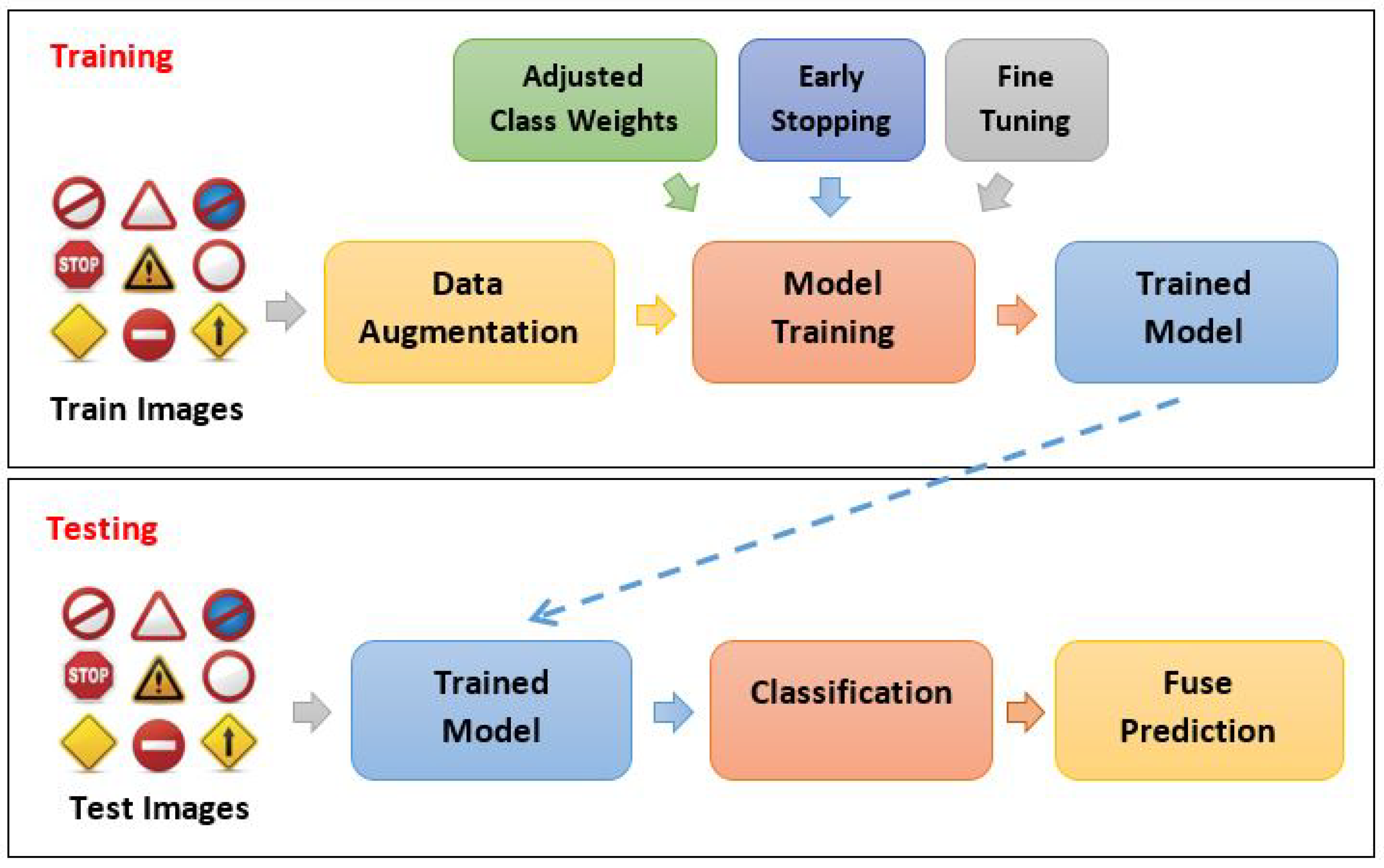
The overall process of the proposed solution is outlined in Figure 1. To begin, data augmentation is applied to increase the size of the training set and address the issue of imbalanced datasets. Next, each of the three CNNs is trained on the augmented training set to learn representations and assess their ability to generalize. The trained models are then used to make predictions on the testing set. Finally, the predictions of all models are fused, using majority voting to determine the final class label.

Figure 1. General pipeline of the proposed traffic sign recognition.

3.1. Data Augmentation

Data augmentation is a widely-used technique in machine learning, that aims to increase the size of the training set by generating new samples based on existing ones. This helps to reduce the risk of overfitting, where the model becomes too specialized to the training data and fails to generalize to new examples. Another important aspect of data augmentation is its ability to balance imbalanced datasets, where one or more classes have a significantly lower number of samples compared to others.

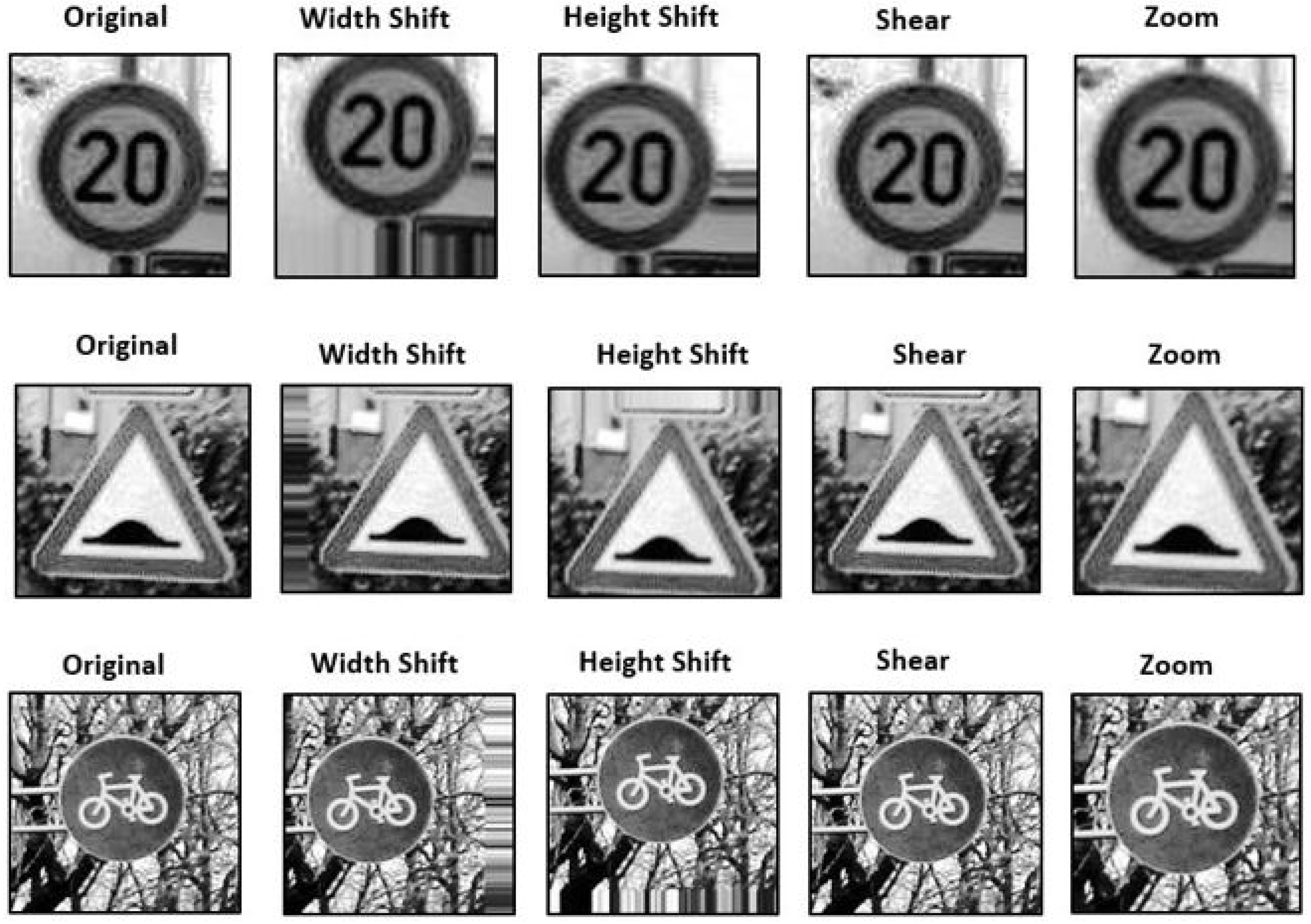
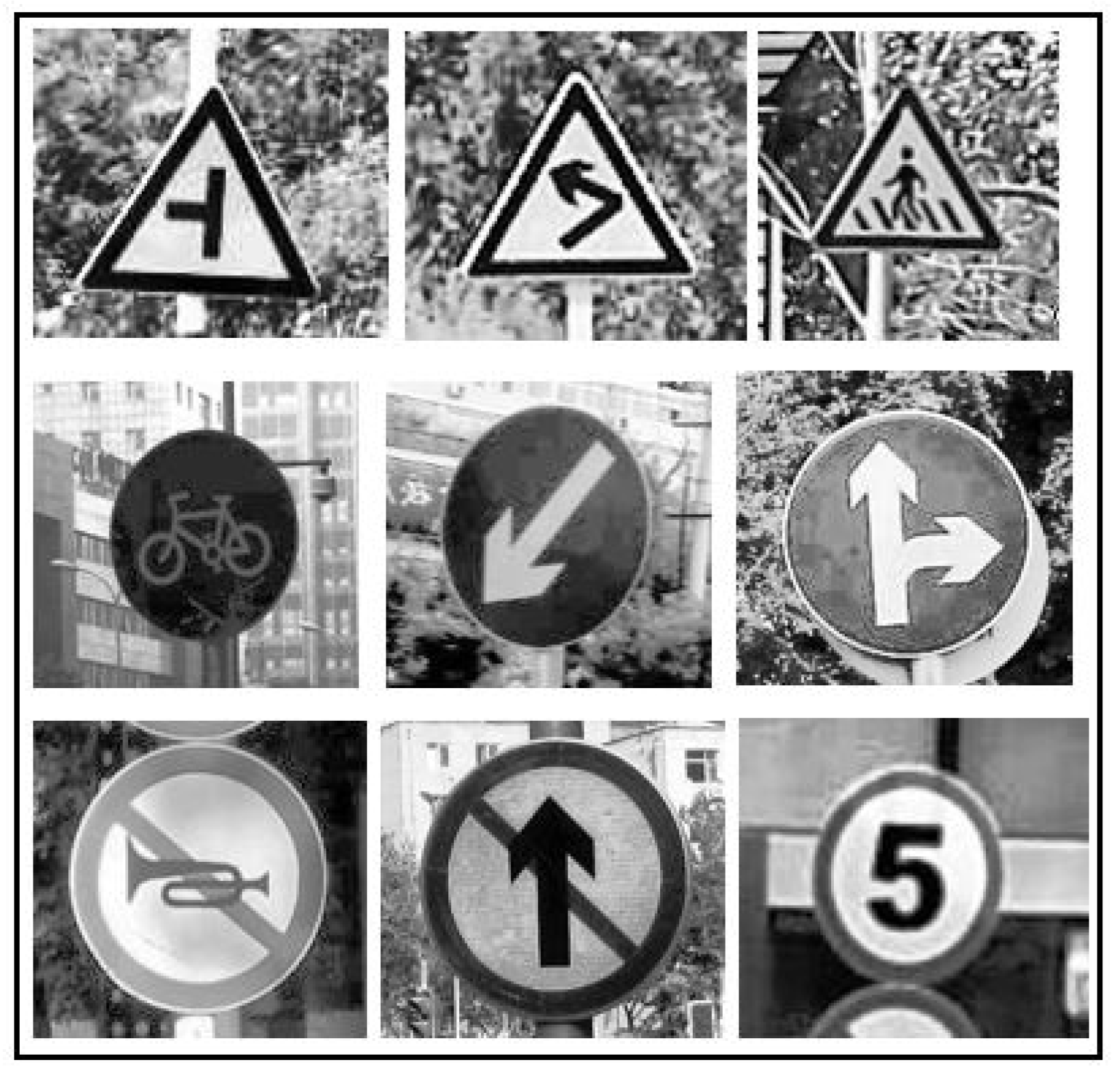
In this work, data augmentation is applied using a set of techniques, including width shift, height shift, brightness adjustment, shear transformation, and zoom. These techniques produce variations of the original samples, thereby increasing the size of the training set and reducing the impact of imbalanced datasets. Figure 2 illustrates some examples of the augmented data.

Figure 2. Sample output images of data augmentation techniques on GTSRB (top row), BTRD (middle row), and TSRD (bottom row).

• Width shift: The image undergoes a horizontal shift, and the range for the width shift is set to 0.2. This means the image will be randomly shifted by a value between +0.2 times the image width and −0.2 times the image width. Positive values will move the image to the right, and negative values will move the image to the left.
• Height shift: The image undergoes a vertical shift, either upwards or downwards. The range of the height shift is set to 0.2, which means the shift will be from −0.2 times the image width to +0.2 times the image width. Positive values selected randomly will result in an upward movement of the image, whereas negative values will result in a downward movement.
• Shear: Shear refers to the process of warping an image along one axis, to change or create perceived angles. The range for shear is set to 0.2, which means the shear angle will be 20 degrees when viewed counterclockwise.
• Zoom: The zoom function allows for zooming in to or out of an image. A value less than 1 will result in enlarging the image, while a value greater than 1 will result in zooming out. The range for zoom is set to 0.2, meaning that the image will be zoomed in.
• Fill mode: This defines the approach to be taken for filling the pixels that were shifted outside the input region. The default fill mode is “nearest”, which fills the empty pixels with values from the nearest non-empty pixel.

3.2. Ensemble Model

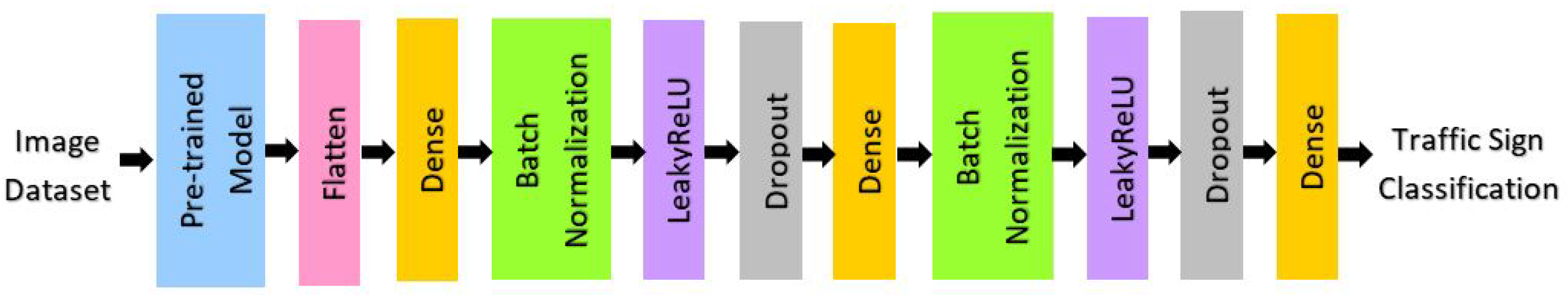
In the proposed method, several pre-trained CNN models, including ResNet50, VGG16, and DenseNet121, are utilized as the backbone. After each pre-trained model, a flatten layer is added, followed by two blocks that consist of a dense layer, a batch normalization layer, a leakyReLU activation layer, and a dropout layer. The model is concluded with a classification layer. Figure 3 displays the architecture of each model.

Figure 3. The architecture of the proposed CNN pre-trained model.

3.3. Pre-Trained Models

ResNet50 is a 50-layer deep CNN that is a variation of the ResNet architecture. It consists of 48 convolution layers, a max pool layer, and an average pool layer. ResNet50 is known for its ability to learn rich image features for a wide range of images. Additionally, the network has a unique characteristic of not requiring all neurons to fire in every epoch, making it computationally efficient.

VGG16 is a 16-layer deep CNN that has a large number of parameters, with a total of over 138 million. Despite its size, VGG-16 has a simple architecture and has proven to perform well on various applications and datasets outside of ImageNet.

DenseNet121 is a part of the DenseNet family and has 8 million parameters. Unlike other networks, it utilizes the concept of residual connections, where the output from preceding layers is concatenated instead of summed. Furthermore, DenseNet121 has a large number of dense connections, enabling the network to effectively utilize all of the preceding layer’s feature maps as input for the subsequent layers.

3.3.1. Flatten Layer

The generated 2-dimensional arrays from pooling feature maps are all flattened into a single, long continuous linear vector.

3.3.2. Dense Layer

A dense layer is one in which each neuron is connected to every other neuron in the preceding layer. In this type of layer, each neuron in the current layer receives input from every neuron in the preceding layer. This input is multiplied with weights, and a bias term is added, before passing through an activation function. In a model, the last dense layer typically has an activation function, such as softmax, which is used for multi-class classification tasks. The number of units in a dense layer can be set to any value, but in the proposed model, it is set to 512.

3.3.3. Batch Normalization

The batch normalization layer normalizes the inputs. The layer uses a transformation to maintain the mean and standard deviation of the output near 0 and 1, respectively. It is important to note that batch normalization exhibits different behavior during inference compared to training.

3.3.4. LeakyReLU

Leaky ReLU is a variant of the popular rectified linear unit (ReLU) activation function. It is used in deep learning models to introduce non-linearity into the activation of neurons. The function is defined as:

$$f\left(x\right)=max(\alpha x,x)$$

(1)

where $\alpha$ is a small positive value, typically 0.01. If the input x is positive, then the output is equal to x, just like in a traditional ReLU. If the input x is negative, then the output is $\alpha x$, which is a small, non-zero value. This allows the network to still propagate some gradient during backpropagation, even when x is negative, which can help to mitigate the issue of “dead neurons” in a model. In this work, the $\alpha$ is set to 0.2.

3.3.5. Dropout Layer

The dropout layer randomly sets input units to 0, with a probability of ‘rate’ during training, to prevent overfitting. Non-zero inputs are scaled up by 1/(1 − rate), to maintain the total sum of inputs. In the proposed model, the dropout rate is set to 0.3.

The CNN architecture is presented in Table 2, including the name of each layer and the corresponding hyperparameter settings. The proposed model has a total of 11 layers.

Table 2. Layer name and hyperparameter settings of CNN.

Layer Name	Hyperparameter Settings
Pre-trained Model	weights = “imagenet”, input_shape = (64,64,3), include_top = false
Flatten	-
Dense	Units = 512
Batch normalization	-
LeakyReLU	Alpha = 0.2
Dropout	Rate = 0.3
Dense	Units = 512
Batch normalization	-
LeakyReLU	Alpha = 0.2
Dropout	Rate = 0.3
Dense	Units = number of classes, activation = softmax

3.4. Optimization for Model Training

In the model training process, class weight balancing is achieved through oversampling, which increases the instances of classes with fewer samples, to match the class with the most samples. To prevent overfitting and reduce training time, early stopping is used. This technique automatically terminates training when a selected performance metric reaches a plateau. Fine tuning is also performed, to optimize model performance.

3.5. Classification and Prediction Fusion

The trained CNN model is evaluated on a test dataset, to determine its accuracy in classifying images. During the classification process, the model learns from the training data for each category (prohibitory, danger, mandatory, etc.) and makes predictions on the test data. To improve prediction accuracy, the outputs of multiple models are combined through majority voting. This technique selects the class with the most votes, where a class must receive over 50% of the votes to be considered the prediction. Empirically, majority voting has been shown to be an effective method for combining classifier predictions.

4. Datasets

This project uses the GTSRB [22], BTSD [23], and TSRD datasets for performance evaluation. These datasets, sourced from online sources, are suitable for traffic sign recognition and contain multiple classes. These three datasets are used to train and test the proposed models. Before use, all datasets were converted to grayscale and histogram equalization was applied.

4.1. German Traffic Sign Recognition Benchmark (GTSRB)

The GTSRB dataset was collected by the Institut für Neuroinformatik and published by Johannes Stallkamp, Marc Schlipsing, Jan Salmen, and Christian Igel. It contains 51,839 images, belonging to 43 different traffic sign classes, including danger, prohibitory, mandatory, and others. The original images are in PPM format and the dataset is imbalanced, so oversampling is performed. After oversampling, the dataset consists of 96,659 images, with 80,108 images used for training, 3921 images used for validation, and 12,630 images used for testing. Figure 4 shows some sample images of the GTSRB dataset.

Figure 4. Sample images of the GTSRB dataset.

4.2. Belgium TS Dataset (BTSD)

The BTSD was publicly hosted and released by VISICS, ESAT, and KU Leuven. It consists of 7095 images, belonging to 62 different classes of traffic signs, which were originally in PPM format and were converted to JPG. Due to some classes having a limited number of images, data cleaning was performed to remove those classes. After cleaning and oversampling, to balance the dataset, the BTSD consists of 20,646 images with 53 classes. Some sample images of the BTSD are presented in Figure 5.

Figure 5. Sample images of the BTSD dataset.

4.3. Chinese Traffic Sign Database (TSRD)

The TSRD was acknowledged by the National Nature Science Foundation of China (NSFC) through a grant. It consists of 6,164 traffic sign images and has 58 classes. The images were collected using Baidu Street View or cameras in natural settings, and captured under a variety of conditions, including different weather, lighting, and partial occlusion. Data cleaning and oversampling were performed to address the imbalance in the dataset. Finally, the TSRD dataset has 24,989 images with 57 classes, with 22,550 images used for training, 439 images used for validation, and 200 images used for testing. Figure 6 provides some sample images of the TSRD dataset.

Figure 6. Sample images of the TSRD dataset.

Table 3 presents the number of samples in the datasets before and after data augmentation. The description of each dataset is summarized in Table 4.

Table 3. Number of samples before and after oversampling.

Dataset	Number of Samples
	Before Oversampling	After Oversampling
GTSRB	51,839	96,659
BTSD	7095	20,646
TSRD	6164	24,989

Table 4. Summary of datasets.

Dataset	Samples	Classes	Training Samples	Validation Samples	Testing Samples
GTSRB	96,659	43	80,108	3921	12,630
BTSD	20,646	53	17,657	469	2520
TSRD	24,989	57	22,550	439	2000

5. Hyperparameter Tuning

Hyperparameter tuning is an essential step in the development of deep learning models, as it involves selecting the most optimal set of hyperparameters to maximize the performance of the model. In this study, three key hyperparameters were chosen for tuning: batch size, learning rate, and optimizer.

The batch size was tested with three different values, namely 16, 32, and 64. The learning rate was tested with three values, 0.001, 0.0001, and 0.00001. Finally, three optimizers were used in the tuning process, namely Adam, stochastic gradient descent (SGD), and adaptive gradient algorithm (AdaGrad). The best hyperparameter values were determined based on the highest test accuracy on the GTSRB dataset.

Table 5 presents the results of the hyperparameter tuning experiment. As shown in the table, a batch size of 64 was found to produce the highest accuracy of 98.84%. The use of the Adam optimizer, and a learning rate of 0.001, also contributed to the optimal results.

Table 5. Summary of hyperparameter tuning.

Hyperparameters	Tested Values	Optimal Value
Batch size	32, 64, 128	64
Learning rate	0.001, 0.0001, 0.00001	0.001
Optimizer	Adam, SGD, Adagrad	Adam

It is noteworthy to mention, that the choice of batch size plays a crucial role in determining the accuracy of deep learning systems. This is due to the fact that batch size affects the estimation of the error gradient, which is a crucial component in the optimization of deep learning models. A larger batch size may speed up processing time, as GPUs can utilize more data, but it also increases the risk of poor generalization, as demonstrated in Table 6. Therefore, it is essential to strike a balance between batch size and accuracy, to ensure the optimal performance of deep learning systems.

Table 6. Traffic sign recognition accuracy (%) at different batch sizes (L = 0.001, O = Adam).

Batch Size (B)	Accuracy (%)
32	98.78
64	98.84
128	98.45

The learning rate is a critical hyperparameter, that plays a pivotal role in determining the performance of a deep learning model. It acts as a multiplier that controls the step size at each iteration of the optimization algorithm, thereby affecting the pace at which the model approaches the optimal weights.

The value of the learning rate has a direct impact on the optimization process and the ultimate performance of the deep learning model. If the learning rate is set too high, the model may overstep the optimal solution and result in unstable convergence. On the other hand, if the learning rate is too low, the optimization process may take an excessively long time to reach the optimal weights.

The results of the hyperparameter tuning experiment showed that the best accuracy was achieved with a learning rate of 0.001. This value strikes a delicate balance between the pace of convergence and stability, ensuring that the optimization process converges to the optimal weights in an efficient manner. The results of the hyperparameter tuning experiment shown in Table 7, suggest that a learning rate of 0.001 is an effective value, that provides a good balance between convergence speed and stability.

Table 7. Traffic sign recognition accuracy (%) at different learning rates (B = 64, O = Adam).

Learning Rate (L)	Accuracy (%)
0.001	98.84
0.0001	98.59
0.00001	97.81

The Adam optimizer is a widely used optimization algorithm in deep learning, based on the stochastic gradient descent method. It is a unique optimization algorithm that updates the learning rate for each network weight individually, taking into account the historical gradient information.

The Adam optimizer combines the benefits of the RMS Prop and Adagrad algorithms, making it a versatile optimization algorithm with several advantages. Firstly, it requires minimal tuning, making it easy to implement and use. Secondly, it is computationally efficient and has a low memory requirement, making it ideal for large-scale deep learning models.

These advantages have contributed to the popularity of the Adam optimizer and its widespread use in deep learning publications. In the case of the proposed ensemble learning model, the use of the Adam optimizer resulted in the highest accuracy of 98.84%, as shown in Table 8.

Table 8. Traffic sign recognition accuracy (%) with different optimizers (B = 64, L = 0.001).

Optimizer (O)	Accuracy (%)
Adam	98.84
SGD	97.22
AdaGrad	97.08

6. Experimental Results and Analysis

This section presents the experimental results of the proposed ensemble learning method, which was applied to the GTSRB, BTSD, and TSRD datasets, and compared with existing traffic sign classification algorithms. The performance of the individual models and the proposed ensemble learning method was evaluated based on various metrics such as accuracy, precision, recall, and F1 score.

The performances of the individual models, as well as the proposed ensemble learning method, in terms of accuracy, precision, recall, and F1 score, are shown in Table 9, Table 10 and Table 11. On the GTSRB dataset, the ensemble learning model achieved a higher F1 score of 98.84%, compared to the F1 score of the individual models, where ResNet50 achieved 97.37%, DenseNet121 achieved 97.38%, and VGG16 achieved 98.02%.

Table 9. Accuracy, precision, recall, and F1 score on GTSRB.

	GTSRB
	Accuracy (%)	Precision (%)	Recall (%)	F1 Score (%)
ResNet50	96.59	97.37	97.37	97.37
DenseNet121	97.54	97.38	97.38	97.38
VGG16	96.59	98.02	98.02	98.02
Ensemble learning	98.84	98.84	98.84	98.84

Table 10. Accuracy, precision, recall, and F1 score on BTSD.

	BTSD
	Accuracy (%)	Precision (%)	Recall (%)	F1 Score (%)
ResNet50	97.37	97.62	97.62	97.62
DenseNet121	97.37	97.34	97.34	97.34
VGG16	99.25	96.98	96.98	96.98
Ensemble learning	98.33	98.33	98.33	98.33

Table 11. Accuracy, precision, recall, and F1 score on TSRD.

	TSRD
	Accuracy (%)	Precision (%)	Recall (%)	F1 Score (%)
ResNet50	88.45	88.45	88.45	91.05
DenseNet121	95.45	95.45	95.45	90.25
VGG16	89.65	89.65	89.65	81.35
Ensemble learning	96.16	96.16	96.16	96.16

On the BTSD dataset, the F1 scores of ResNet50, DenseNet121, and VGG16 were 97.62%, 97.34%, and 96.98%, respectively. The ensemble learning method again outperformed the individual models, with an accuracy of 98.33%. The improvement in performance can be attributed to the fact that the ensemble learning method is more robust and less sensitive to noise in the data, which is an important characteristic of real-world datasets.

On the TSRD dataset, ResNet50, DenseNet121, and VGG16 recorded F1 scores of 91.05%, 90.25%, and 81.35%, respectively. By fusing the predictions of the models, the F1 score increased to 96.16%. The improvement demonstrates that the ensemble learning method is able to mitigate the wrong predictions of individual models and improve the overall performance. The ensemble learning method is also more robust to the high inter-class similarity in the TSRD, which is a major challenge in traffic sign classification.

One of the main reasons why the ensemble learning method outperformed the individual models, is that it combines the predictions of multiple models. The ensemble method is able to mitigate the weaknesses of individual models by taking into account their predictions and fusing them into a single prediction. This reduces the risk of making wrong predictions, that individual models may make due to their own biases or limitations.

6.1. Comparative Results with the Existing Works

The experimental results presented in Table 12 demonstrate that the proposed ensemble learning method outperforms existing deep learning techniques, in terms of accuracy, on the GTSRB dataset. CNN-based models, including CNN [6], ENet [8], CNN [11], CNN [12], MCNN [15], and CNN [17], achieved recognition rates ranging from 96.00% to 98.60%, while ViT [16] achieved an accuracy of 98.82%. The unsupervised LBP model [5] had an accuracy of 95.00%.

Table 12. Comparative results on GTSRB dataset.

Method	Accuracy (%)
LBP [5]	95.00
CNN [6]	97.40
ENet [8]	98.60
CNN [11]	96.00
CNN [12]	98.44
MCNN [15]	98.26
ViT [16]	98.82
CNN [17]	97.80
Ensemble Learning	98.84

The proposed ensemble learning method achieved an accuracy of 98.84%, which is higher than all the other individual models and ViT. This shows that by combining the predictions of multiple pre-trained CNN models, the ensemble learning method is able to achieve improved performance compared to the individual models. The optimized combination of models, batch sizes, learning rates, and other hyperparameters, contributes to the overall success of the ensemble, resulting in a superior accuracy rate.

Table 13 presents the comparison of current approaches with ensemble learning on the BTSD dataset. The accuracy of the deep learning algorithms NCC [7], CNN [9], CNN [6], and ELM [20] on the dataset were 93.10%, 97.06%, 98.10%, 98.30%, and 98.37%, respectively. The proposed ensemble learning method achieved a higher classification rate, of 98.33%, on the BTSD dataset, compared to existing approaches. The proposed method improved accuracy by combining three CNN models in the ensemble layer.

Table 13. Comparative results on BTSD dataset.

Method	Accuracy (%)
CNN [6]	98.10
NCC [7]	93.10
CNN [9]	97.06
ELM [20]	98.30
Ensemble Learning	98.33

On the TSRD dataset, Table 14 compares the experimental results of the current methods and ensemble learning. It can be observed that, in terms of accuracy, the proposed method outperforms the machine learning approaches on the TSRD dataset. One of the main causes is that, TSRD consists of the most classes, as compared to the other datasets, therefore it will be more complicated to classify. The existing methods used are only using one model, thus, ensemble learning with the combination of three models will give a better performance. The proposed method achieved 96.16% accuracy, which is much improved compared to the existing methods.

Table 14. Comparative results on TSRD dataset.

Method	Accuracy (%)
SVM [21]	84.44
CNN [6]	60.30
CNN [12]	70.70
CNN [24]	36.87
Ensemble Learning	96.16

6.2. Confusion Matrices

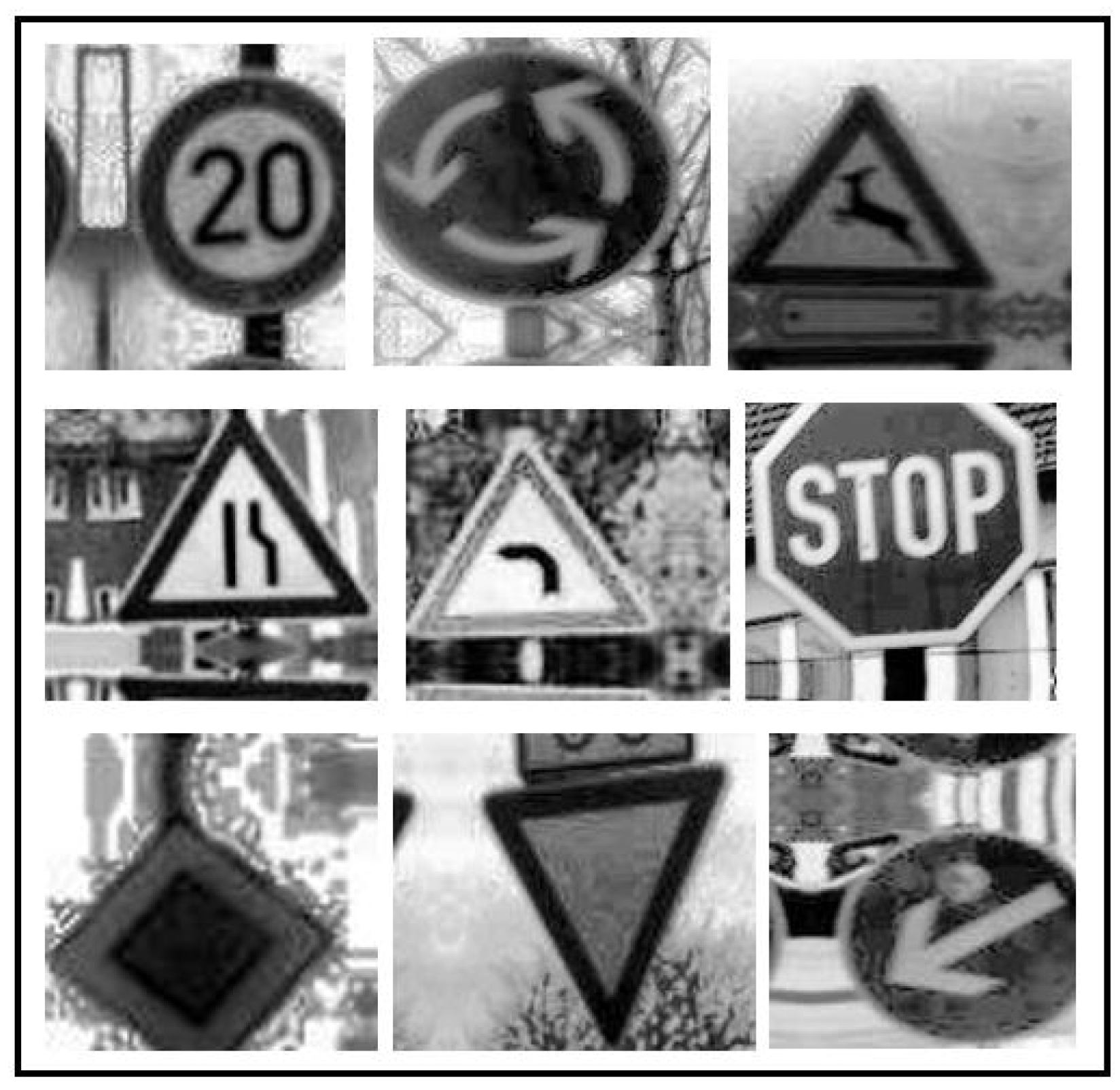
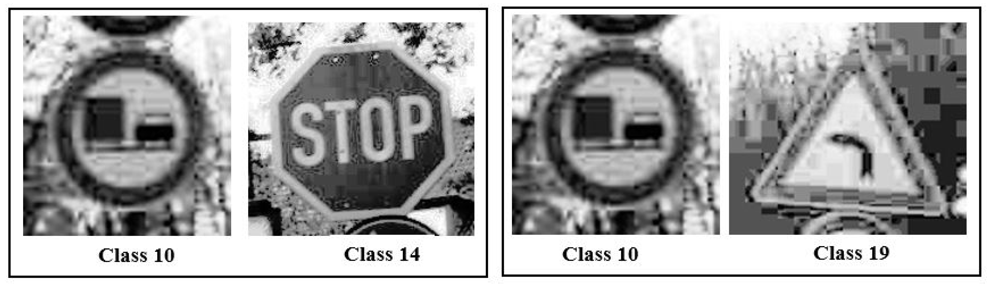
Figure 7 presents the confusion matrix for the proposed ensemble learning model, on the GTSRB dataset.The blue shade in the confusion matrix indicates the true positive values, with deeper shades representing higher values. According to the confusion matrix, classes 10 and 14 have the highest misclassification rates. The second highest misclassification rates are between classes 10 and 19. These high rates are likely due to the presence of background noise in the traffic sign images, which impacts the classification. Examples of misclassified classes can be seen in Figure 8.

Figure 7. Confusion matrix of ensemble learning on the GTSRB dataset.

Figure 8. Misclassified classes of 10 and 14 (left) and 10 and 19 (right).

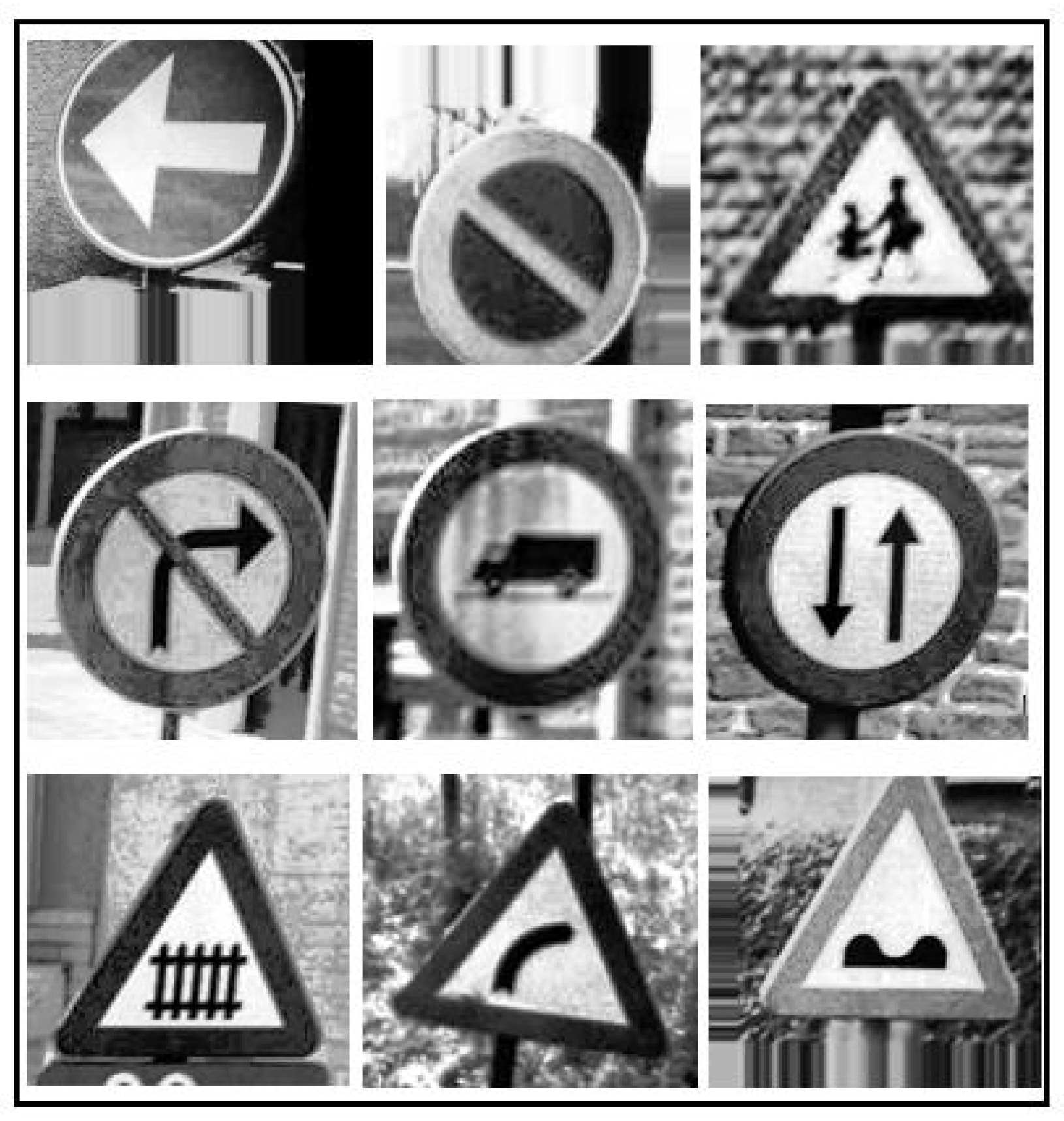
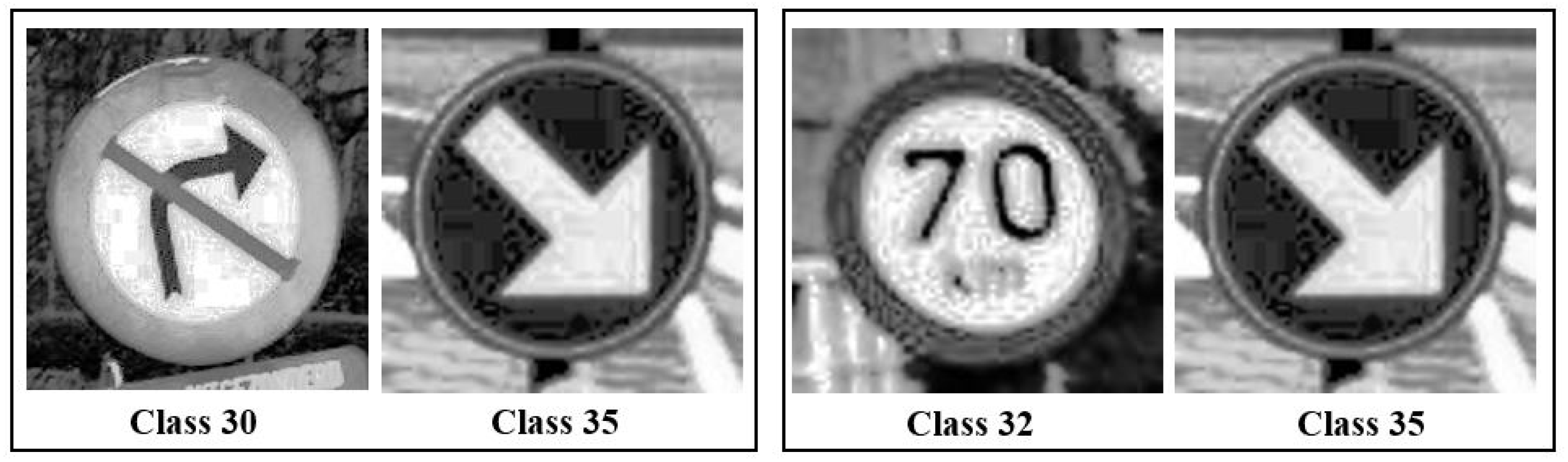
The confusion matrix of the ensemble learning model on the BTSD is depicted in Figure 9. The highest misclassified classes, classes 30 and 35, and the second-highest misclassified classes, between classes 32 and 35, are possibly due to the similarities in the shapes (circles) and symbols of the traffic signs for classes 30 and 35. Samples of the misclassified classes can be viewed in Figure 10.

Figure 9. Confusion matrix of ensemble learning on the BTSD dataset.

Figure 10. Misclassified classes of 30 and 35 (left) and 32 and 35 (right).

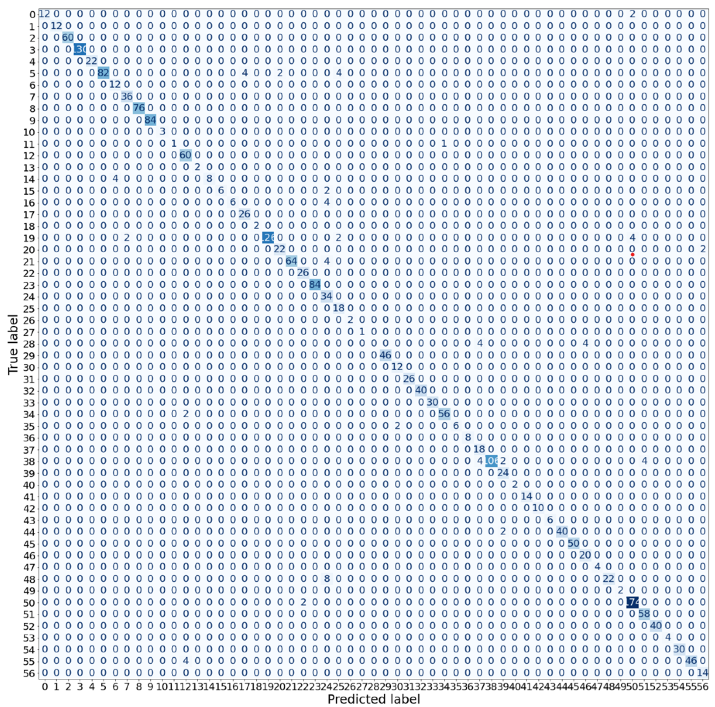
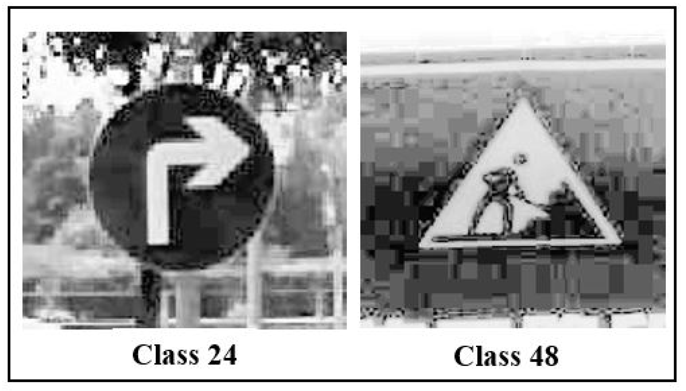
According to the confusion matrix in Figure 11, it is evident that the highest misclassified classes in the TSRD dataset are classes 24 and 48. Similar to the GTSRB dataset, traffic signs that are circular or triangular in shape are frequently misclassified. The samples of these misclassified classes are depicted in Figure 12.

Figure 11. Confusion matrix of ensemble learning on the TSRD dataset.

Figure 12. Misclassified classes of 24 and 48.

7. Conclusions

This paper propose an ensemble learning deep learning model for traffic sign classification. Ensemble learning involves combining several models to produce a more accurate result, compared to relying on a single model. This approach not only improves the accuracy but also enhances the robustness of the model, by reducing its performance variability and prediction dispersion. To implement the ensemble model, the researchers utilized three pre-trained deep learning models: ResNet50, DenseNet121, and VGG16. The proposed ensemble model was evaluated on three different traffic sign datasets: the GTSRB dataset, the BTSR dataset, and the TSRD dataset. The results showed that the proposed ensemble learning model outperforms existing traffic sign classification techniques, with recognition rates of 98.84% on the GTSRB dataset, 98.33% on the BTSR dataset, and 94.55% on the TSRD dataset. Attention-based models, especially the vision transformer, have shown significant advancements in image recognition tasks. Therefore, future research can investigate the effectiveness of attention-based models for traffic sign recognition, by exploring their potential advantages and addressing their challenges. This can contribute to advancing the state-of-the-art in traffic sign recognition and provide new insights into the application of attention-based models in computer vision tasks.