
Cognitive Risk-Assessment and Decision-Making Framework for Increasing in-Vehicle Intelligence


 ,
,
Abstract
1. Introduction
2. Motivation and High-Level Description
2.1. Intelligent Vehicles
2.2. Risk Assessment
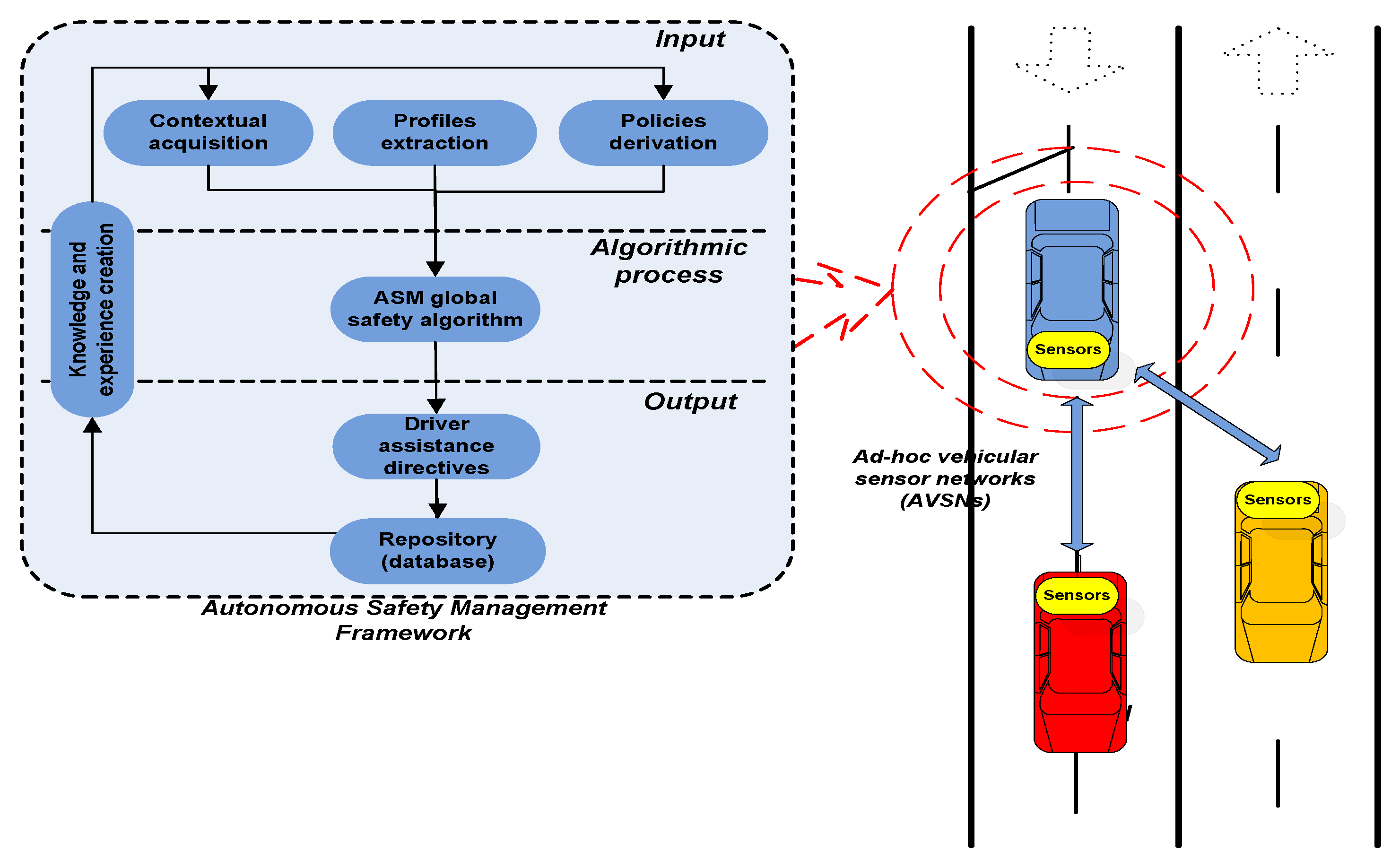
2.3. High-Level Description
- (a)
- assessing traffic information in a real-time manner through aggregating and federating information from sensors embedded in the vehicle,
- (b)
- considering a set of potential decisions applying a novel, cognitive heuristic
- (c)
- associating each of the candidate’s decisions with potential risks and therefore influencing the solutions space,
- (d)
- increasing the embedded intelligence of a vehicle through a holistic safety approach, with the use of in-vehicle sensors
3. Problem Description and Solution
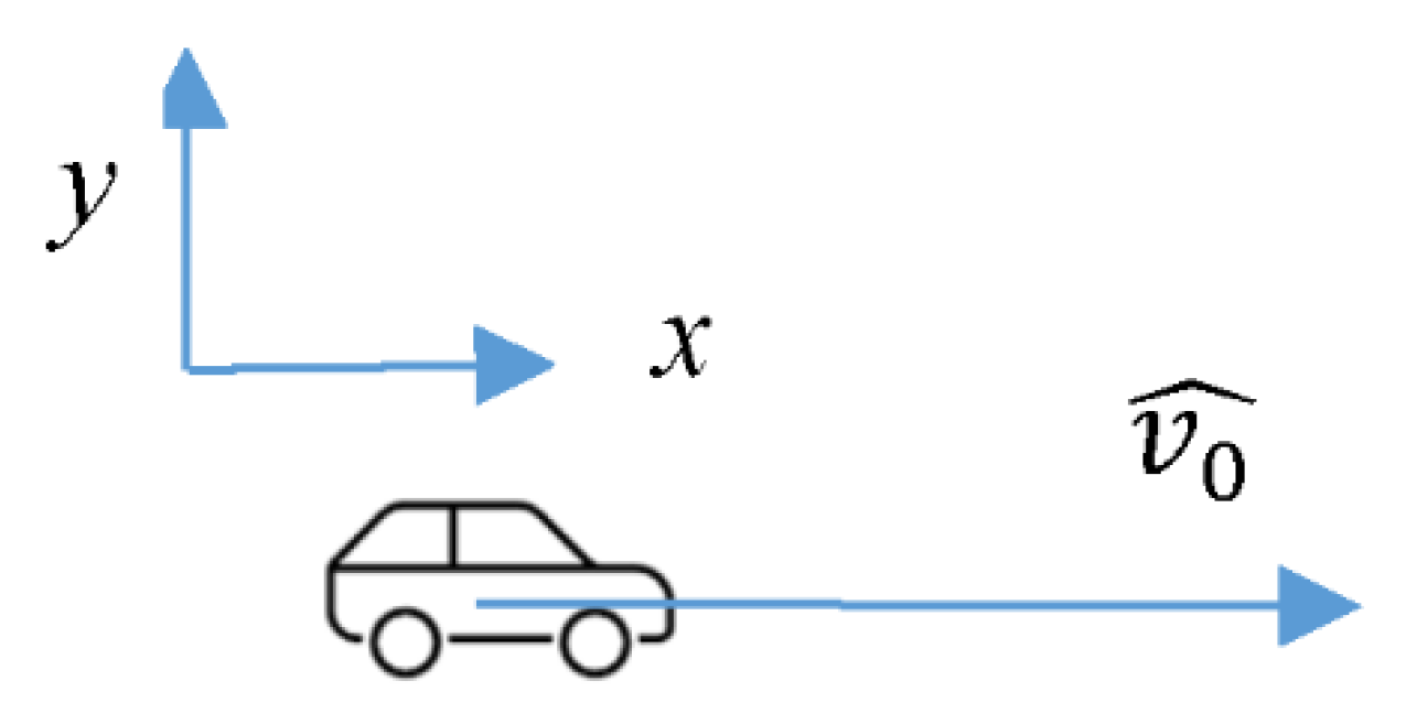
3.1. Context Modeling
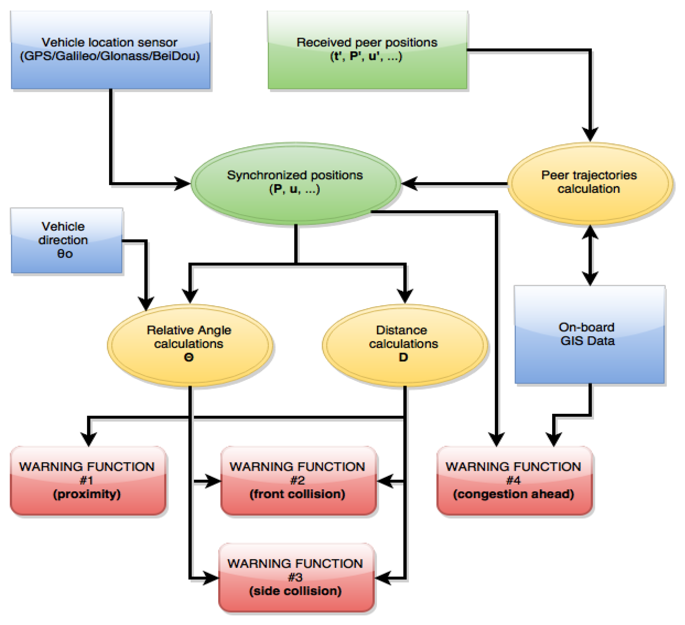
3.2. Solution Approach: Warning Functions
3.2.1. Least Safety Distance Warning
3.2.2. Safe following Distance Warning
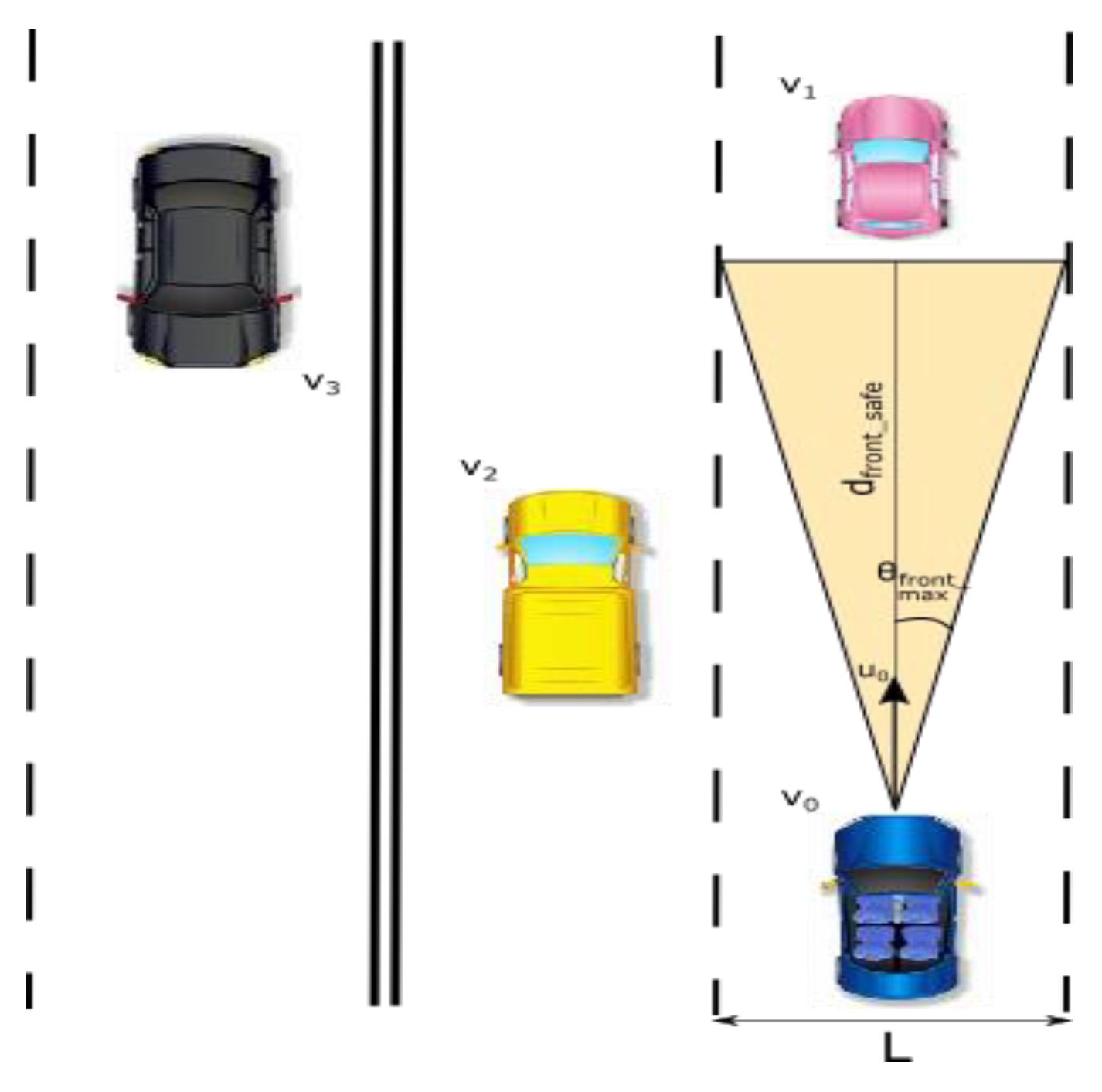
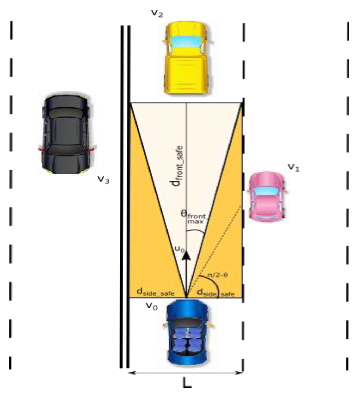
3.2.3. Safe Front-Side Distance Warning

3.2.4. Congestion Ahead Warning
4. Simulation Results
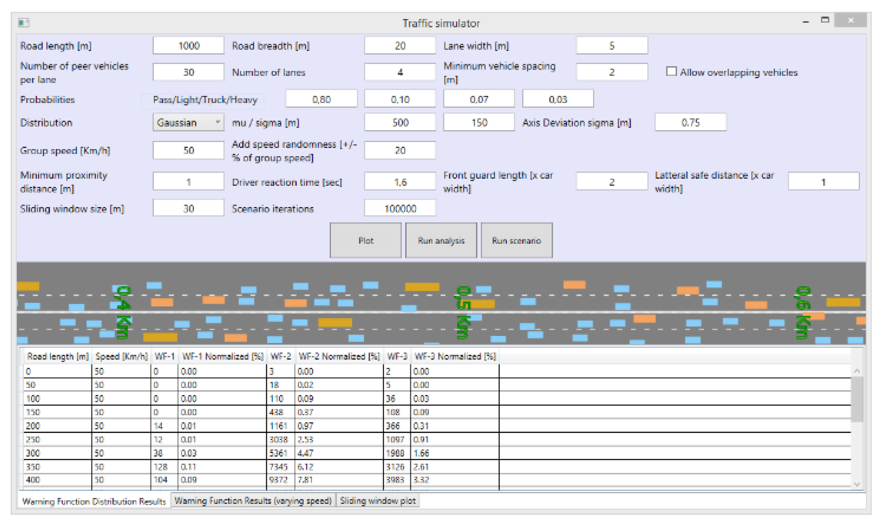
4.1. Simulator Setup
4.2. Results
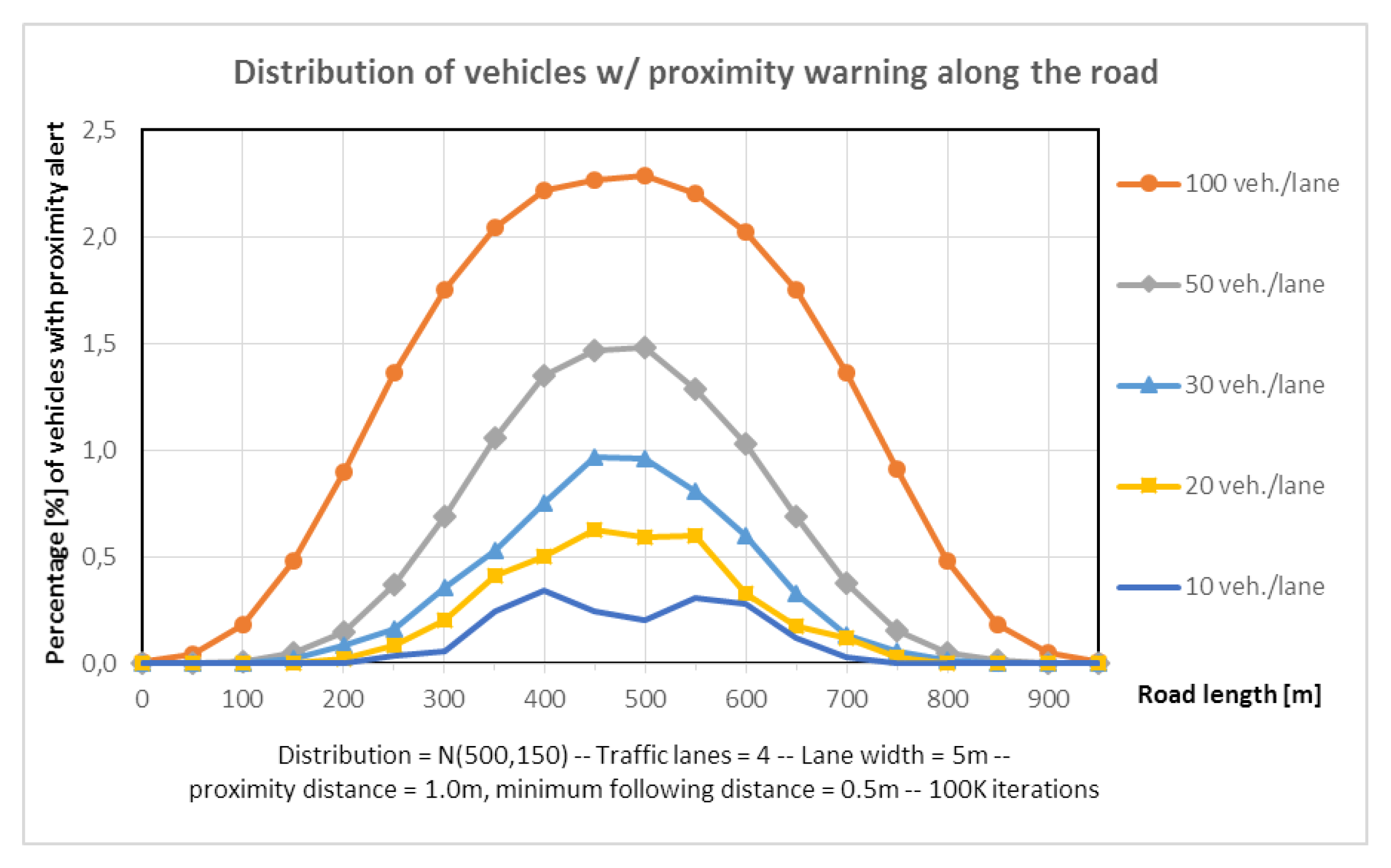
- Warning Function 1—Proximity Warning
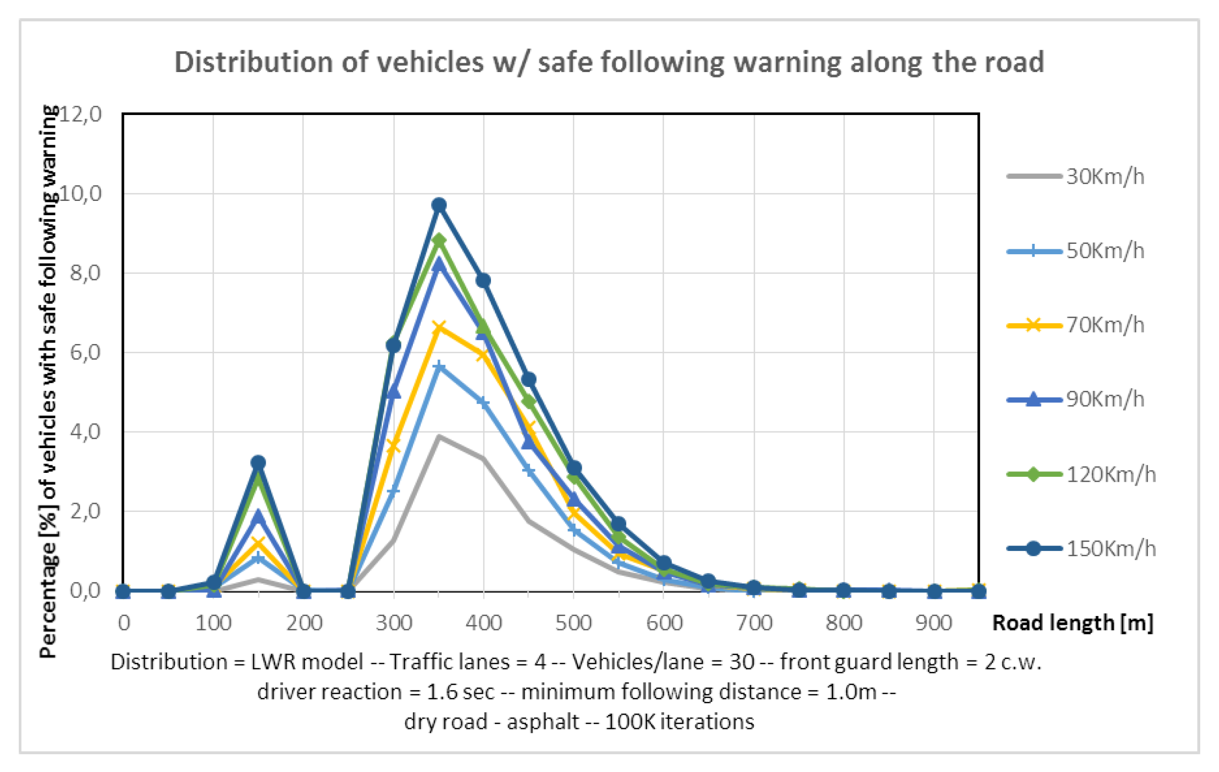
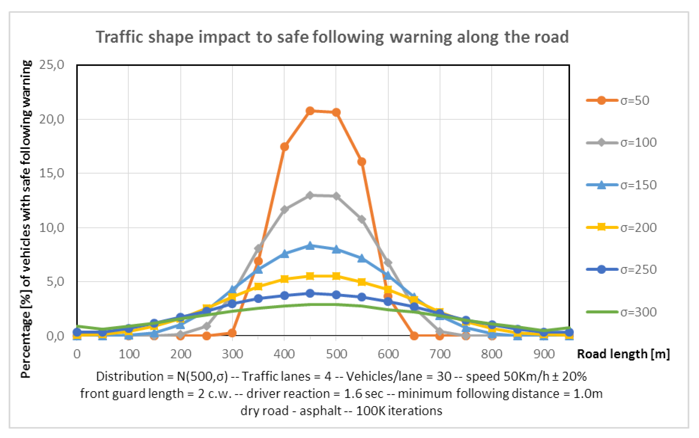
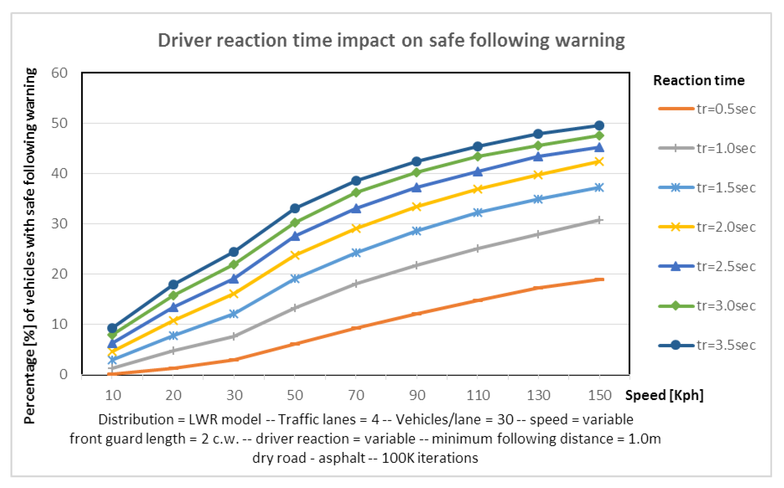
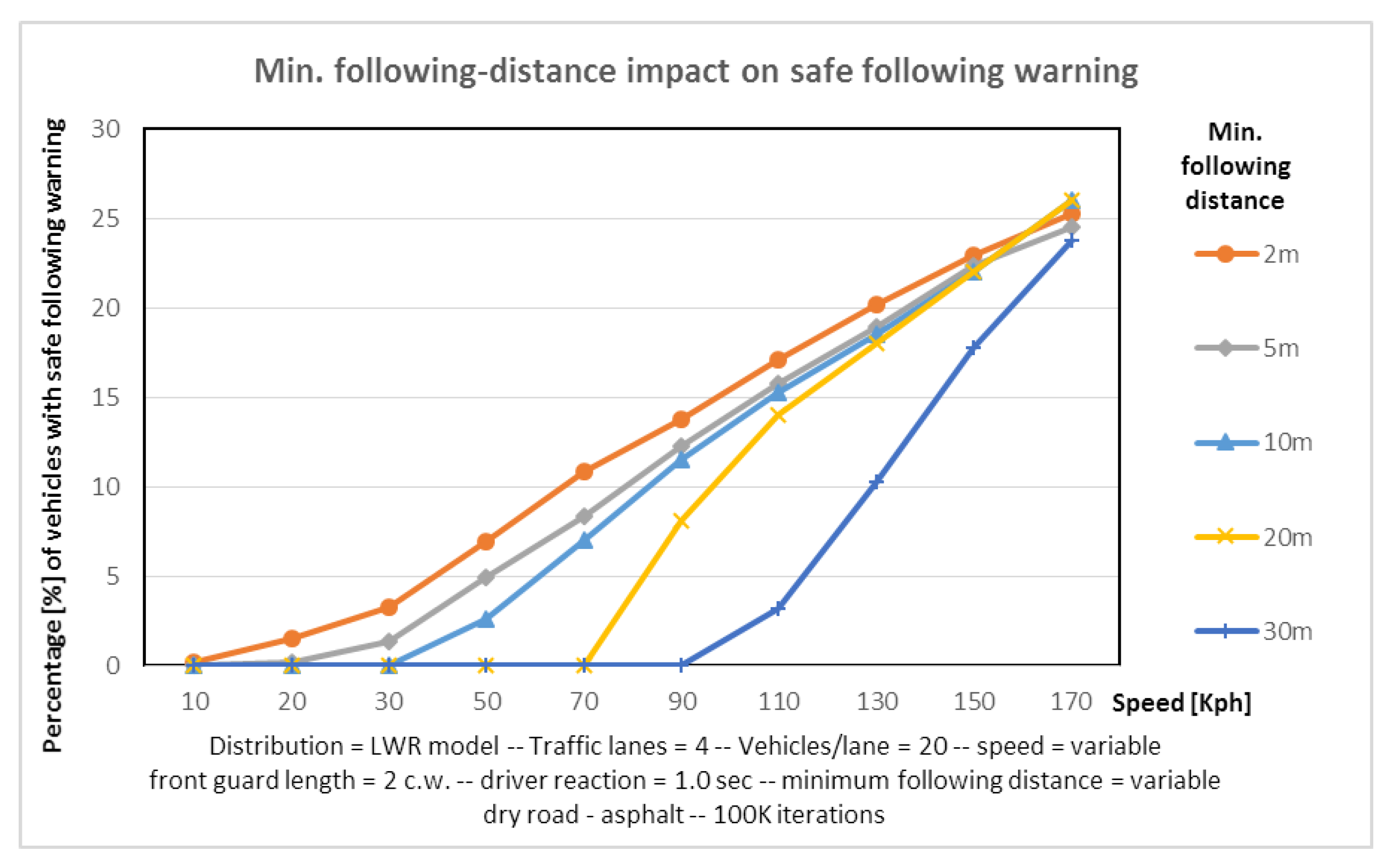
- Warning Function 2—Safe following Distance Warning
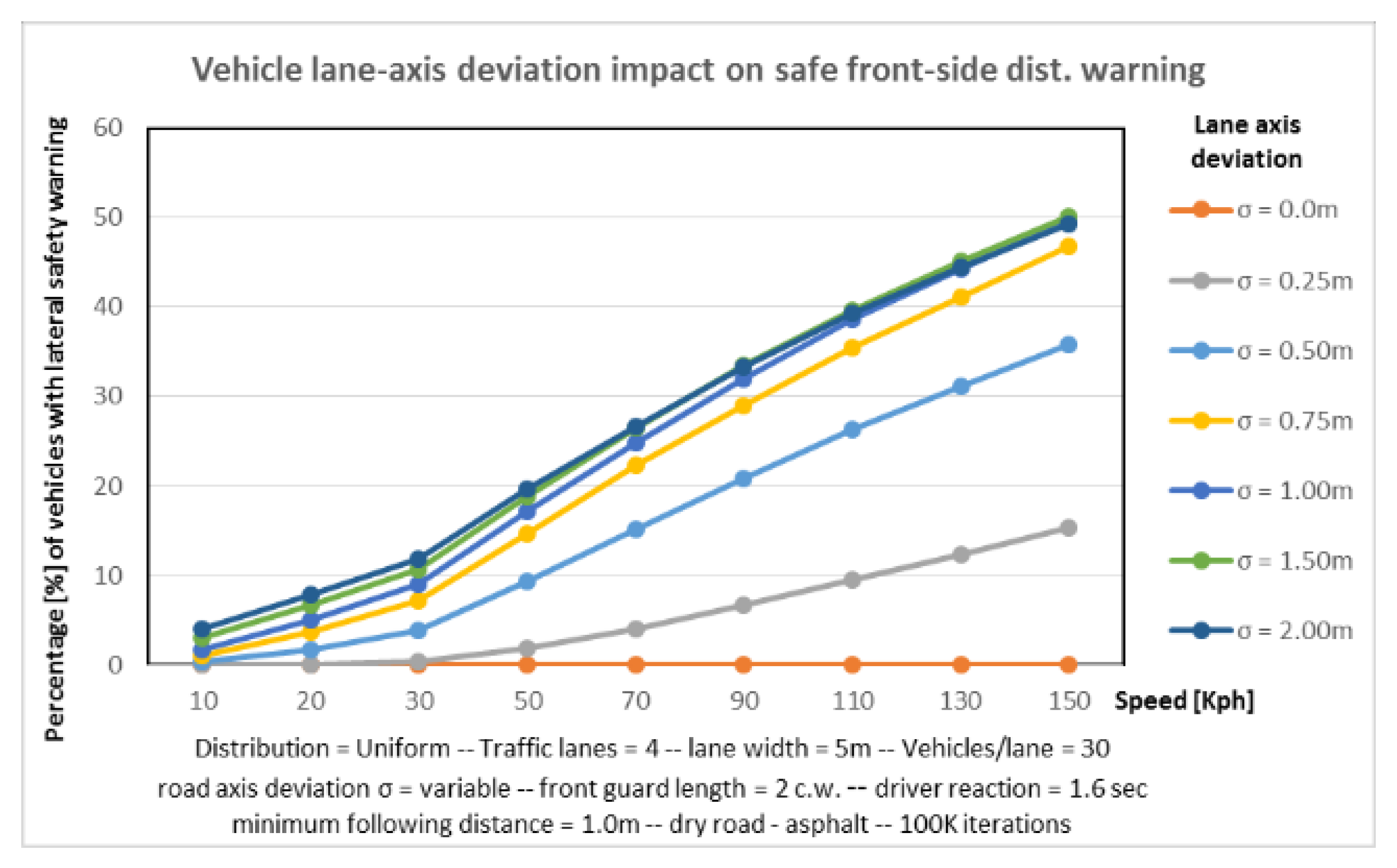
- Warning Function 3—Safe Front-Side Distance Warning
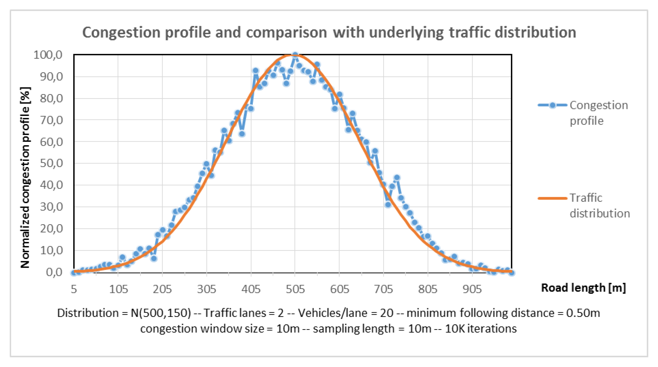
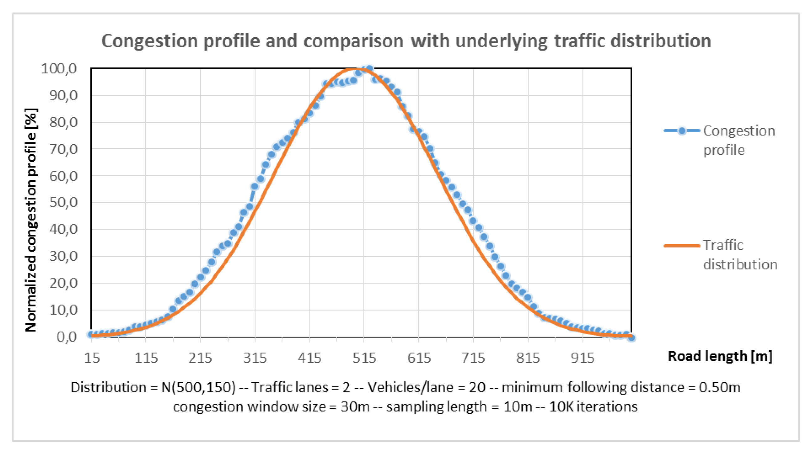
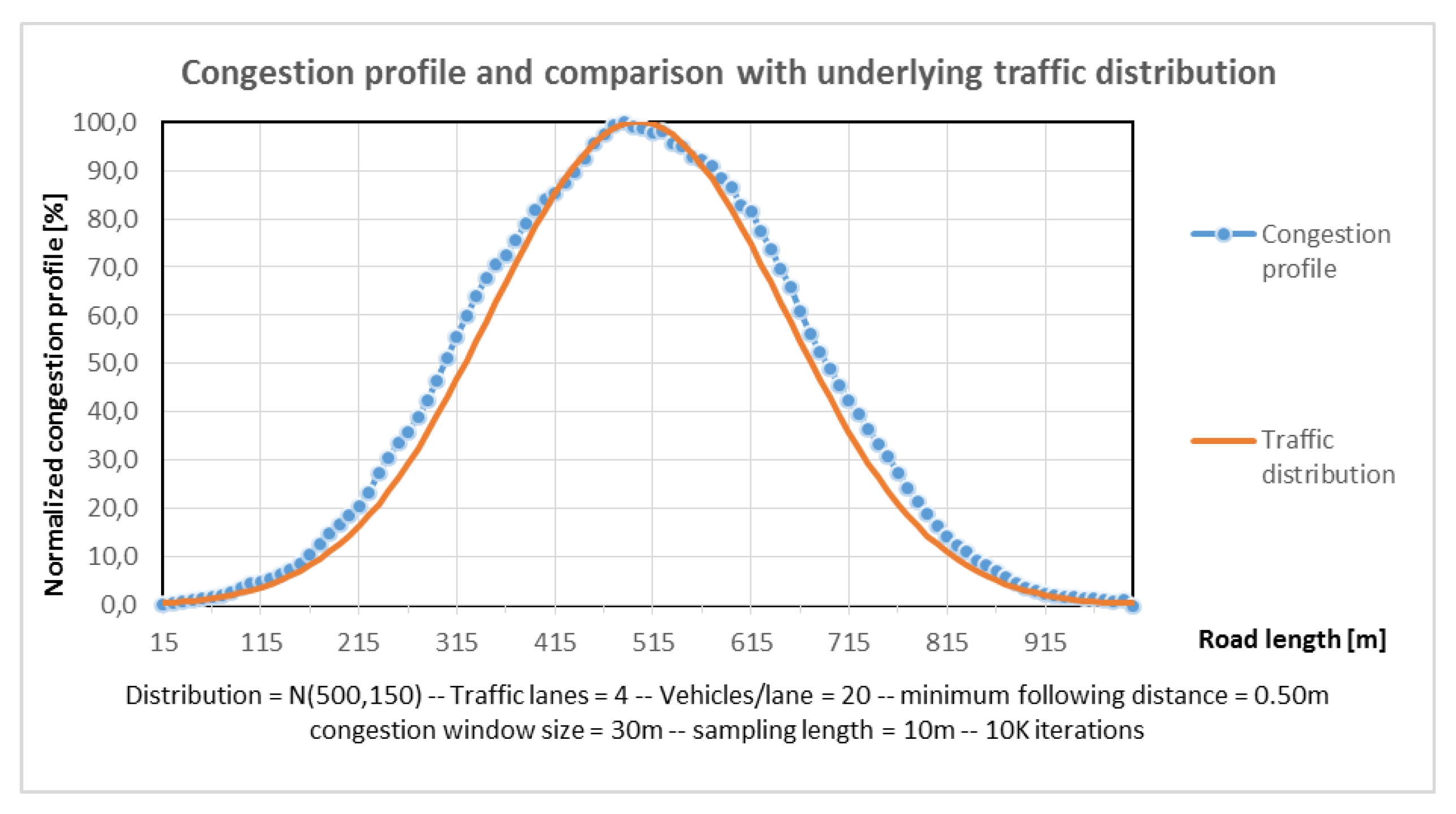
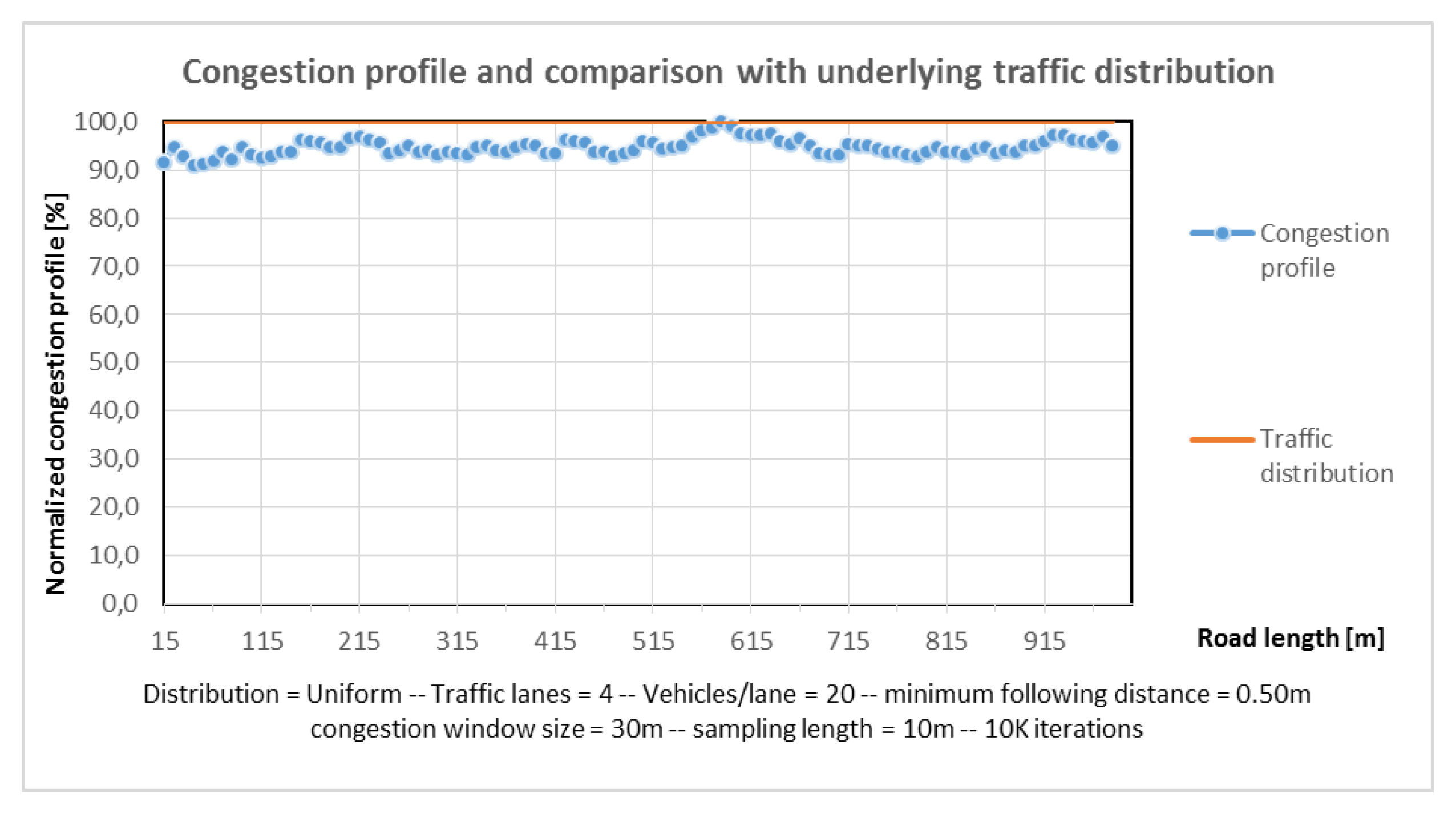
- Warning Function 4—Congestion ahead warning
5. Conclusions and Future Directions
Author Contributions
Funding
Institutional Review Board Statement
Informed Consent Statement
Data Availability Statement
Conflicts of Interest
References
- Rocha Filho, G.P.; Meneguette, R.I.; Neto, J.R.T.; Valejo, A.; Weigang, L.; Ueyama, J.; Pessin, G.; Villas, L.A. Enhancing intelligence in traffic management systems to aid in vehicle traffic congestion problems in smart cities. Ad. Hoc. Netw. 2020, 107, 102265. [Google Scholar] [CrossRef]
- United Nations. Transforming Our World: The 2030 Agenda for Sustainable Development. Available online: https://sustainabledevelopment.un.org/content/documents/21252030%20Agenda%20for%20Sustainable%20Development%20web.pdf (accessed on 10 July 2022).
- United Nations. The 17 Goals. Available online: https://sdgs.un.org/goals (accessed on 15 July 2022).
- European Commission. EU Road Safety Policy Framework 2021–2030-Next Steps towards Vision Zero. Available online: https://ec.europa.eu/transport/sites/transport/files/legislation/swd20190283-roadsafety-vision-zero.pdf (accessed on 15 July 2022).
- Zographos, T.; Dimitrakopoulos, G.; Anagnostopoulos, D. Driver Assistance through an Autonomous Safety Management Framework. In Proceedings of the IEEE Wireless and Mobile Communications (WiMOB) 2016, New York, NY, USA, 17–19 October 2016. [Google Scholar]
- Lu, N.; Cheng, N.; Zhang, N.; Shen, X.; Mark, J.W. Connected Vehicles: Solutions and Challenges. IEEE Internet Things J. 2014, 1, 289–299. [Google Scholar] [CrossRef]
- Sedjelmaci, H.; Senouci, S.M.; Abu-Rgheff, M.A. An Efficient and Lightweight Intrusion Detection Mechanism for Service-Oriented Vehicular Networks. IEEE Internet Things J. 2014, 1, 570–577. [Google Scholar] [CrossRef]
- Zhu, Y.H.; Luan, S.; Leung, V.C.; Chi, K. Enhancing Timer-Based Power Management to Support Delay-Intolerant Uplink Traffic in Infrastructure IEEE 802.11 WLANs. IEEE Trans. Veh. Technol. 2015, 64, 386–399. [Google Scholar] [CrossRef]
- Schakel, W.J.; van Arem, B. Improving Traffic Flow Efficiency by In-Car Advice on Lane, Speed, and Headway. IEEE Trans. ITS 2014, 15, 1597–1606. [Google Scholar] [CrossRef]
- Na, X.; Cole, D.J. Game-Theoretic Modeling of the Steering Interaction Between a Human Driver and a Vehicle Collision Avoidance Controller. IEEE Trans. Hum.-Mach. Syst. 2015, 45, 25–38. [Google Scholar] [CrossRef]
- Lin, J.R.; Talty, T.; Tonguz, O.K. A Blind Zone Alert System Based on Intra-Vehicular Wireless Sensor Networks. IEEE Trans. Ind. Inform. 2015, 11, 476–484. [Google Scholar] [CrossRef]
- Sun, Y.; Chowdhury, K. Enabling emergency communication through a cognitive radio vehicular network. IEEE Commun. Mag. 2014, 52, 68–75. [Google Scholar] [CrossRef]
- Lee, W.H.; Lai, Y.C.; Chen, P.Y. A Study on Energy Saving and CO2 Emission Reduction on Signal Countdown Extension by Vehicular Ad Hoc Networks. IEEE Trans. Veh. Technol. 2015, 64, 890–900. [Google Scholar] [CrossRef]
- Dimitrakopoulos, G.; Bravos, G.; Nikolaidou, M.; Anagnostopoulos, D. A Proactive, Knowledge-Based Intelligent Transportation System based on Vehicular Sensor Networks. IET Intell. Transp. Syst. J. 2013, 7, 454–463. [Google Scholar] [CrossRef]
- Lin, J.R.; Talty, T.; Tonguz, O.K. On the potential of bluetooth low energy technology for vehicular applications. IEEE Com. Mag. 2015, 53, 267–275. [Google Scholar] [CrossRef]
- Dimitrakopoulos, G.; Ghattas, J. Autonomic Decision Making for Vehicles based on Visible Light Communications. In Proceedings of the 14th Wireless Telecommunications Symposium (WTS) 2015, New York, NY, USA, 15–17 April 2015. [Google Scholar]
- Ferreira, M.; d’Orey, P.M. On the Impact of Virtual Traffic Lights on Carbon Emissions Mitigation. IEEE Trans. ITS 2012, 13, 284–295. [Google Scholar] [CrossRef]
- Sinha, R.; Roop, P.; Ranjitkar, P. Virtual Traffic Lights+: A Robust, Practical, and Functionally Safe Intelligent Transportation System. Transp. Res. Rec. 2013, 2381. [Google Scholar] [CrossRef]
- Bellotti, F.; Berta, R.; Kobeissi, A.; Osman, N.; Arnold, E.; Dianati, M.; Nagy, B.; De Gloria, A. Designing an IoT Framework for Automated Driving Impact Analysis. In Proceedings of the 2019 IEEE Intelligent Vehicles Symposium (IV), Paris, France, 9–12 June 2019; pp. 1111–1117. [Google Scholar] [CrossRef]
- An, D.; Liu, J.; Zhang, M.; Chen, X.; Chen, M.; Sun, H. Uncertainty Modeling and Runtime Verification for Autonomous Vehicles Driving Control: A Machine Learning-based Approach. J. Syst. Softw. 2020, 167, 110617. [Google Scholar] [CrossRef]
- Panagiotopoulos, I.; Karathanasopoulou, K.; Dimitrakopoulos, G. Risk Assessment in the Context of Dynamic Reconfiguration of Driving Automation Level in Highly Automated Vehicles. In Proceedings of the 7th IEEE Conference on Computational Science & Computational Intelligence (CSCI), Las Vegas, NV, USA, 15–17 December 2021. [Google Scholar]
- Yan, L.; Wu, C.; Zhu, D.; Ran, B.; He, Y.; Qin, L.; Li, H. Driving Mode Decision Making for Intelligent Vehicles in Stressful Traffic Events. Transp. Res. Rec. J. Transp. Res. Board 2017, 2625, 9–19. [Google Scholar] [CrossRef]
- Panagiotopoulos, K.I.; Karathanasopoulou, G. Dimitrakopoulos, Risk based Decision Making Functionality for Improving the Level of Autonomy Reconfiguration in Automated Vehicles. In Proceedings of the ITS World Congress 2022, Los Angeles, NV, USA, 18–22 September 2022. [Google Scholar]
- Li, X.; Zhang, X.; Ren, X.; Fritsche, M.; Wickert, J.; Schuh, H. Precise positioning with current multi-constellation Global Navigation Satellite Systems: GPS, GLONASS, Galileo and BeiDou. Sci. Rep. 2015, 5, 8238. [Google Scholar] [CrossRef] [PubMed]
- Jenny, B. Adaptive Composite Map Projections. IEEE Trans. Vis. Comp. Graph. 2012, 18, 2575–2582. [Google Scholar] [CrossRef] [PubMed]
- Press, W.H.; Teukolsky, S.A.; Vetterling, W.T.; Flannery, B.P. Numerical Recipes, 3rd ed.; Cambridge Press: Cambridge, UK, 2007; pp. 1122–1124. [Google Scholar]
- Green, M. “How long does it take to stop?” Methodological Analysis of Driver Perception-Brake Times. Transp. Human Factors 2000, 2, 195–216. [Google Scholar] [CrossRef]
- Xing, C.F.; Yang, L.; Zhang, Y.H. Study of driver’s reaction time (DRT) during car following. In Applied Mechanics and Materials; Trans Tech Publications Ltd.: Wollerau, Switzerland, 2015; Volume 713–715. [Google Scholar]
- D’Addario, P.M. Perception-Response Time to Emergency Roadway Hazards and the Effect of Cognitive Distraction; University of Toronto: Toronto, ON, Canada, 2014. [Google Scholar]
- Wong, J.Y. Theory of Ground Vehicles, 4th ed.; Wiley: Hoboken, NJ, USA, 2008. [Google Scholar]
- Robert Bosch GmbH. Automotive Handbook, 9th ed.; Robert Bosch GmbH: Gerlingen, Germany, 2014. [Google Scholar]
- Treiber, M.; Kesting, A. Traffic Flow Dynamics: Data, Models and Simulation; Springer: Berlin/Heidelberg, Germany, 2013. [Google Scholar]
- Edwards, D.J.; Holt, G.D.; Spittle, P.G. Guidance on Brake Testing for Rubber-Tyred Vehicles Operating in Quarries, Open Cast Coal Sites and Mines. 2007. Available online: https://www.osti.gov/etdeweb/biblio/21396714 (accessed on 15 July 2022).


| Detection | Likelihood of Detection | Di Ranking | Status |
|---|---|---|---|
| Absolute uncertainty | Design control cannot detect potential cause/ mechanism | 10 | Red |
| Very remote | Very remote chance the control will detect potential cause/ mechanism | 9 | Red |
| Remote | Remote chance the control will detect potential cause/ mechanism | 8 | Red |
| Very low | Very low chance the control will detect potential cause/ mechanism | 7 | Red |
| Low | Low chance the control will detect potential cause/ mechanism | 6 | Red |
| Moderate | Moderate chance the control will detect potential cause/ mechanism | 5 | Yellow |
| Moderately high | Moderately high chance the control will detect potential cause/ mechanism | 4 | Yellow |
| High | High chance the control will detect potential cause/ mechanism | 3 | Green |
| Very high | Very high chance the control will detect potential cause/ mechanism | 2 | Green |
| Almost certain | Almost certain the control will detect potential cause/ mechanism | 1 | Green |
| Risk Priority Number | Risk Mitigation Possibility |
|---|---|
| 513–1000 | Very High |
| 217–512 | High |
| 65–216 | Medium |
| 9–64 | Low |
| 0–8 | Improbable |
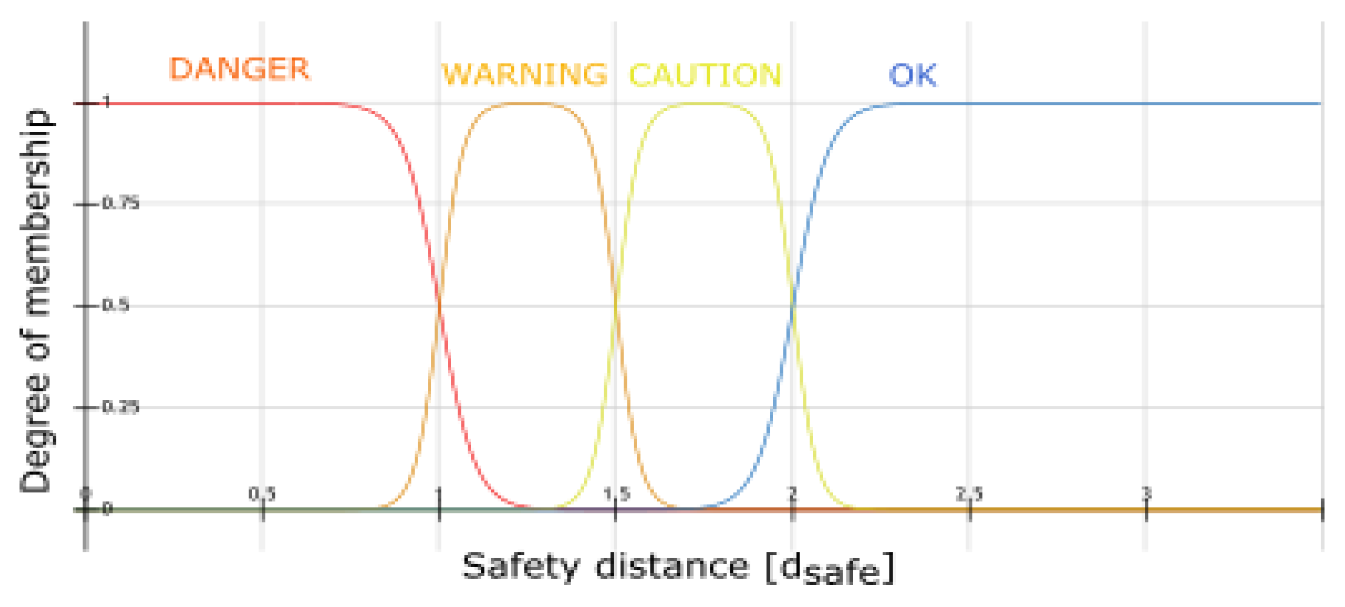
| Safe Distance | |
|---|---|
| “Danger” | |
| “Warning” | |
| “Caution” | |
| “OK” |
| Membership Function | |
|---|---|
| “Danger” | |
| “Warning” | |
| “Caution” | |
| “OK” |
| Road Surface | Peak Value | Sliding Value |
|---|---|---|
| Asphalt and concrete (dry) | 0.80–0.90 | 0.75 |
| Asphalt (wet) | 0.50–0.70 | 0.45–0.60 |
| Concrete (wet) | 0.80 | 0.70 |
| Gravel | 0.60 | 0.55 |
| Earth road (dry) | 0.68 | 0.65 |
| Earth road (wet) | 0.55 | 0.40–0.50 |
| Snow (hard-packed) | 0.20 | 0.15 |
| Ice | 0.10 | 0.07 |
| Tire Friction Coefficient on Asphalt | ||||||
|---|---|---|---|---|---|---|
| Vehicle Speed (km/h) | Tread Depth (mm) | Road Condition | ||||
| Dry | Wet (Water Depth ≈ 0.2 mm) | Heavy Rainfall (Water Depth ≈ 1 mm) | Puddles (Water Depth ≈ 2 mm) | Ice (Black Ice) | ||
| 50 | New | 0.85 | 0.65 | 0.55 | 0.50 | ≤0.10 |
| 50 | 1.6 | 1.00 | 0.50 | 0.40 | 0.25 | ≤0.10 |
| 90 | New | 0.80 | 0.60 | 0.30 | 0.05 | |
| 90 | 1.6 | 0.95 | 0.20 | 0.10 | 0.05 | |
| 130 | New | 0.75 | 0.55 | 0.20 | 0.00 | |
| 130 | 1.6 | 0.90 | 0.20 | 0.10 | 0.00 | |
Publisher’s Note: MDPI stays neutral with regard to jurisdictional claims in published maps and institutional affiliations. |
© 2022 by the authors. Licensee MDPI, Basel, Switzerland. This article is an open access article distributed under the terms and conditions of the Creative Commons Attribution (CC BY) license (https://creativecommons.org/licenses/by/4.0/).
Share and Cite
Dimitrakopoulos, G.; Politi, E.; Karathanasopoulou, K.; Panagiotopoulos, E.; Zographos, T. Cognitive Risk-Assessment and Decision-Making Framework for Increasing in-Vehicle Intelligence. J. Sens. Actuator Netw. 2022, 11, 72. https://doi.org/10.3390/jsan11040072
Dimitrakopoulos G, Politi E, Karathanasopoulou K, Panagiotopoulos E, Zographos T. Cognitive Risk-Assessment and Decision-Making Framework for Increasing in-Vehicle Intelligence. Journal of Sensor and Actuator Networks. 2022; 11(4):72. https://doi.org/10.3390/jsan11040072
Chicago/Turabian StyleDimitrakopoulos, George, Elena Politi, Konstantina Karathanasopoulou, Elias Panagiotopoulos, and Theodore Zographos. 2022. "Cognitive Risk-Assessment and Decision-Making Framework for Increasing in-Vehicle Intelligence" Journal of Sensor and Actuator Networks 11, no. 4: 72. https://doi.org/10.3390/jsan11040072
APA StyleDimitrakopoulos, G., Politi, E., Karathanasopoulou, K., Panagiotopoulos, E., & Zographos, T. (2022). Cognitive Risk-Assessment and Decision-Making Framework for Increasing in-Vehicle Intelligence. Journal of Sensor and Actuator Networks, 11(4), 72. https://doi.org/10.3390/jsan11040072