Abstract
Accurately estimating leaves’ relative chlorophyll contents (widely represented by Soil and Plant Analysis Development (SPAD) values) across growth stages is crucial for assessing crop health, particularly in regions characterized by varying sowing dates. Unlike previous studies focusing on high-resolution UAV imagery or specific growth stages, this research incorporates satellite-derived texture indices (TIs) into a SPAD value estimation model applicable across multiple growth stages (from tillering to grain-filling). Field experiments were conducted in Jiangsu Province, China, where winter wheat sowing dates varied significantly from field to field. Sentinel-2 imagery was employed to extract vegetation indices (VIs) and TIs. Following a two-step variable selection method, Random Forest (RF)-LassoCV, five machine learning algorithms were applied to develop estimation models. The newly developed model (SVR-RBFVIs+TIs) exhibited robust estimation performance (R2 = 0.8131, RMSE = 3.2333, RRMSE = 0.0710, and RPD = 2.3424) when validated against independent SPAD value datasets collected from fields with varying sowing dates. Moreover, this optimal model also exhibited a notable level of transferability at another location with different sowing times, wheat varieties, and soil types from the modeling area. In addition, this research revealed that despite the lower resolution of satellite imagery compared to UAV imagery, the incorporation of TIs significantly improved estimation accuracies compared to the sole use of VIs typical in previous studies.
1. Introduction
Leaves’ relative chlorophyll content (widely represented by Soil and Plant Analysis Development (SPAD) values), as a key physiological parameter reflecting photosynthetic efficiency, growth status, and the nutritional level of crops, has been widely employed in the assessment of crop health [1,2,3]. In recent years, accumulating research has confirmed that remote sensing (RS) technology possesses significant advantages—such as non-invasiveness and high efficiency—in monitoring crops’ SPAD values, making it an ideal tool for this purpose [4,5]. Although unmanned aerial vehicle (UAV)-based RS has advanced rapidly in the context of high-resolution monitoring, satellite-based RS continues to play a dominant role in field-scale or large-area crop monitoring applications [6].
In Jiangsu Province, China, the agricultural production structure is predominantly characterized by small-scale farmers, with relatively few large-scale agricultural operations. At present, small family farms with an average cultivated area of less than one hectare remain the dominant form of agricultural management in the region [7]. As a consequence, the sowing dates of winter wheat exhibit considerable variation across the area [8]. These variations in sowing time significantly influence the growth and development of winter wheat by altering the duration of sunlight and the accumulation of temperature during different phenological stages. This leads to the asynchronous growth stages of winter wheat in different fields at the same point in time [9].
Previous RS-based studies have primarily focused on developing SPAD value estimation models for winter wheat during specific growth stages under uniform sowing dates [10,11]. While these models may exhibit high estimation accuracy under certain conditions, numerous studies have indicated that their applicability is limited during other growth stages, and that their estimations are often unstable, lacking broad generalizability [12,13,14]. Although these models have shown success in controlled environments, their practical application is significantly constrained in real-world agricultural production, particularly in scenarios with diverse sowing dates. This issue is particularly pronounced in Jiangsu Province, China, where most agricultural fields are managed by small-scale farmers, leading to multiple sowing dates for winter wheat.
Furthermore, crop parameter estimation models developed using data from the entire growth cycle demonstrate more stable performance compared to models based solely on data from specific growth stages [15]. This stability stems from the model’s ability to compensate for discrepancies observed at particular growth stages by integrating observations from other stages [13,16]. Dhillon et al. [17] further assert that employing time series RS imagery yields more reliable and accurate estimates of winter wheat growth parameters than relying on a single image from a specific growth stage.
The estimation of SPAD values generally relies on physical modeling approaches (i.e., the PROSAIL model), empirical modeling, or hybrid methods that combine both. However, numerous parameters in physical models are difficult to obtain, which limits their practical application in crop parameter estimation. While hybrid methods can improve estimation accuracy, their instability remains a critical issue due to the challenge of balancing the interface between inversion algorithms and physical models. In contrast, empirical modeling typically combines vegetation indices (VIs) with machine learning techniques to develop regression models. This approach is preferred for SPAD value estimation due to its stability and higher estimation reliability. However, solely relying on VIs significantly limits the development of a comprehensive SPAD value estimation model for winter wheat throughout its entire growth cycle.
The main issue lies in the fact that when VIs are used for modeling SPAD values, saturation problems often occur, especially in environments with high vegetation cover [18]. Additionally, it is noteworthy that during the grain-filling period, despite lower SPAD values due to the transfer and transport of assimilates, the top spike of the winter wheat canopy remains green 14. The presence of both leaves and spikes in the winter wheat canopy makes the reflectance signal more complex, which introduces significant uncertainty when measuring chlorophyll levels in the canopy’s reflectance spectra. Numerous studies have shown that although VIs exhibit a strong correlation with crop parameters at specific growth stages, they are difficult to extrapolate to other growth stages [19,20]. Consequently, these factors present significant challenges in developing a cross-growth-stage SPAD value estimation model that is applicable throughout the entire growth cycle of winter wheat.
Fortunately, by leveraging the spatial variations in pixel intensity, extracting texture indices (TIs) from RS images can effectively reveal crop canopy structure and geometric features, thereby alleviating this challenge to some extent [21]. For instance, Guo et al. [22] significantly improved the estimation accuracy of maize SPAD values by combining VIs and TIs extracted from multispectral UAV images. However, an extensive literature review reveals that most existing studies have focused on extracting TIs from high-resolution UAV-based RS images, with limited attempts to use texture indices derived from satellite RS images to estimate crop parameters. This disparity arises from the significantly lower resolution of satellite RS imagery compared to UAV imagery, leading previous studies to generally perceive accurate crop parameter estimation from satellite RS images as a major challenge [14].
This study aimed to develop a satellite imagery-based model for the accurate estimation of SPAD values that incorporates multiple growth stages of winter wheat. We hypothesized that the capability of satellite-derived TIs enabled this model to be effectively applied in regions with temporal variations in sowing dates. This research represents the first attempt to estimate winter wheat SPAD values using TIs extracted from satellite RS imagery.
2. Materials and Methods
2.1. Study Area
The research was carried out from 2022 to 2023. As depicted in Figure 1, the study area consists of two sub-study areas, namely Huaisi Town (32°31′18″ N, 119°28′6″ E) and Touqiao Town (32°17′31″ N, 119°39′37″ E), both located in Yangzhou City, Jiangsu Province, China.
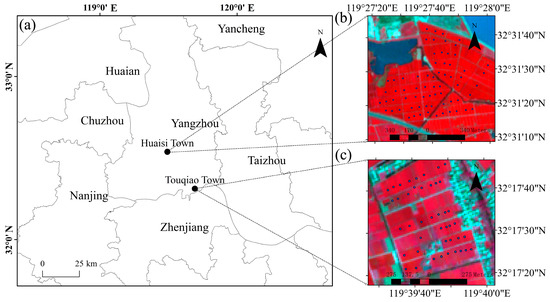
Figure 1.
Geographic location and sampling site distribution of the study area. (a) The geographical locations of the sub-study areas of Huaisi Town and Touqiao Town; (b) the spatial distribution of sampling sites in Huaisi Town, overlaying a false-color composite image (Bands 8, 4, and 3 of Sentinel-2A) acquired on 11 April 2023; and (c) the spatial distribution of sampling sites in Touqiao Town, overlaying a false-color composite image (Bands 8, 4, and 3 of Sentinel-2A) acquired on 8 April 2023.
It is particularly noteworthy that the measured fields in Huaisi Town in this research are cultivated by individual smallholder farmers, with significant variations in fertilization and irrigation practices. The soil type of the fields is sandy loam soil [23]. Conversely, the measured fields in Touqiao Town are cultivated uniformly by much bigger farm owners, with consistent fertilization and irrigation management practices. The soil type of the fields is mucky soil.
These two sub-study areas are located in the mid-lower Yangtze River area and predominantly employ a rice–wheat rotation system. For a long time, the sowing time for winter wheat in the mid-lower Yangtze River area has been affected by tight rice stubble, often resulting in uncertainty [24]. Upon on-site investigation, it was observed that the growth of winter wheat in Huaisi Town (with the variety Yangmai 29) and Touqiao Town (with the variety Zhenmai 18) is not synchronized, particularly evident from significant differences during the vegetative growth stage of winter wheat. For instance, in general, the wheat crops in Huaisi Town and Touqiao Town were observed to be at the heading stage and jointing stage, respectively, on April 10, 2023. Furthermore, the total sowing period in Huaisi Town was stratified into three phenologically distinct phases (normal, intermediate, and late), with inter-phase intervals averaging around 20 days, despite the predominance of winter wheat cultivation occurring during the conventional sowing window.
2.2. Data Collection
2.2.1. Measured SPAD Values for Winter Wheat
In the sub-study area of Huaisi Town, the measured SPAD values of winter wheat were obtained at the growth stages of tillering, green-up, heading, and grain-filling. In the sub-study area of Touqiao Town, the measured SPAD values were obtained at the growth stages of jointing and grain-filling.
Typically, the measurement of SPAD values was conducted on the uppermost fully expanded leaves at different growth stages, as they represented significant variations in SPAD values among individual plants [25,26]. In the vegetative growth stage of winter wheat (tillering, green-up, and jointing), SPAD values offered crucial insights into the crop’s nutritional status, facilitating timely nitrogen fertilizer supplementation. During the reproductive growth stage (heading and grain-filling stages), SPAD values provided highly precise forecasts of yield [27].
At each sampling site, which was 20 m long and 20 m wide, 25 winter wheat plants were randomly chosen for actual SPAD value measurements, employing the non-destructive and portable SPAD-502plus handheld chlorophyll meter (Minolta Camera Co.; Osaka, Japan). In the initial stages of tillering, green-up, and jointing, data were collected from the top, central, and bottom sections of the second-to-last leaf (i.e., the uppermost fully expanded leaf) of the selected plants. During the heading and grain-filling stages, the flag leaf was measured. The mean of these measurements was used as the measured SPAD value for each selected plant. The SPAD value for each specific field was determined by averaging the actual SPAD value measurements from the 25 selected wheat plants.
2.2.2. Acquisition of Sentinel-2 Images
Field-scale crop monitoring often necessitates high-resolution optical imagery to discern and extract complex crop growth characteristics [28]. It is noteworthy that each sampling plot in this study measured 20 m × 20 m, within which 25 winter wheat plants were randomly selected for in situ SPAD value measurements. Sentinel-2 MSI imagery—with native spatial resolutions of 10 m, 20 m, and 60 m across various bands—was resampled to a consistent 10 m-resolution reflectance dataset. This spatial scale is well aligned with the field plot dimensions, ensuring that each 10 m pixel integrates spectral signals from a physiologically meaningful portion of the canopy. Hence, it provides sufficiently detailed spectral and structural information to estimate SPAD values at the field level [29].
Sentinel-2 MSI imagery data of winter wheat during its crucial growth stages was obtained using the Google Earth Engine (GEE) platform. This platform has given us access to a wide range of satellite RS tools, including Level-1C and Level-2A products from Sentinel-2. The Level-2A product is generated by performing atmospheric correction on the Level-1C product and represents the Surface Reflectance [30]. The frequent revisit rate of Sentinel-2 of every five days [31] allows for the acquisition of at least one cloud-free image during each critical growth stage of winter wheat. This frequent revisit rate significantly enhances the practicality of our research methodology. For this research, the Level-2A product was chosen for subsequent analysis. Table 1 comprehensively lists the specific Sentinel-2 optical satellite imagery data utilized in this research. It is worth noting that the field data collection and model development were initially conducted in Huaisi Town. To further assess the robustness and spatial transferability of the developed model, Touqiao Town was subsequently incorporated as an independent validation site. Although only two cloud-free Sentinel-2 images were available for Touqiao Town, these acquisitions coincided with key growth stages of winter wheat, thereby enabling a representative and meaningful evaluation of model performance.

Table 1.
An inventory of Sentinel-2 MSI imagery was utilized in this study.
2.3. Extraction and Construction of RS Variables
Subsequently, all band data of the sampling points were extracted on the Google Earth Engine (GEE) platform (https://earthengine.google.com/ (accessed on 30 June 2024)), including B1, B2, B3, B4, B5, B6, B7, B8, B8A, B9, B11, and B12, and were resampled to 10 m reflectance data. Subsequently, they were used to calculate the VIs used for estimating SPAD values (Table 2).
Table 2.
RS variables employed in the study.
The Gray-Level Co-occurrence Matrix (GLCM) initially proposed by Haralick in 1973 [52] is a prominent technique for texture analysis. Its popularity stems from variables such as rotational invariance, the capability to operate at multiple scales, and computational efficiency [53]. Acknowledging the influence of spatial resolution on TIs, GLCM-TIs were extracted from single-band images (B2, B3, B4, and B8) at a 10 m resolution on the GEE platform. The glcmTexture function was applied with a 3 × 3 moving window, and the results were averaged across four principal directions (0°, 45°, 90°, and 135°). The TIs used for estimating SPAD values in winter wheat are enumerated in Table 2.
To ensure the comprehensiveness of the input variables, a total of 96 RS variables were constructed, comprising both spectral and spatial information. Specifically, 36 VIs were derived from 12 spectral bands of Sentinel-2 MSI (Level-2A) imagery and their pairwise combinations. Additionally, 60 TIs were extracted from four 10 m resolution bands (B2, B3, B4, and B8) using 15 GLCM-based metrics, thereby capturing the spatial heterogeneity and structural characteristics of the crop canopy.
2.4. Variable Selection Method
Owing to the high-dimensional nature of the feature space (96 RS variables in total), rigorous variable selection must be implemented as a critical preliminary step in the modeling pipeline. However, employing a single variable selection method alone, like most previous studies did, may not effectively identify the most critical variables [54]. By addressing the issue of redundant RS image variables, previous studies have shown that a two-step variable selection process can markedly reduce the variable set without compromising the model’s accuracy, and even enhance the model’s performance [55,56]. Therefore, in this research, a two-step variable selection method, RF-LassoCV (initially using Random Forest for preliminary variable selection followed by LassoCV), was used, with the expectation of reducing data redundancy, optimizing the model, and producing reliable results with high computational efficiency. Variable selection was combined with five-fold cross-validation (CV) in this research.
2.5. Machine Learning Regression Models
Our primary objective in this research was to develop a strong model for accurately estimating the SPAD values of winter wheat from the tillering stage to the grain-filling stage. To achieve this, various machine learning regression models were explored, including RF [57], Support Vector Regression (SVR) [58] with different kernels (SVR-RBF, SVR-Poly, SVR-Sigmoid, and SVR-Linear), CatBoost [59], Backpropagation Neural Network (BPNN) [60], Long Short-Term Memory (LSTM) [61], and ElasticNet [62].
The parameters and non-parameters of these machine learning models were optimized using CV and grid search algorithms. By comparing the performance of these models, the most suitable model for winter wheat SPAD value estimation could be selected.
The specific modeling procedure is illustrated in Figure 2. To interpret the optimal model behavior and evaluate the contribution of each variable to the estimation of the target output (response variable), Shapley Additive Explanations (SHAP) analysis, as proposed by Lundberg and Lee [63], was utilized. It is important to emphasize that SHAP values do not infer causality; instead, they provide insights into the optimal model’s behavior in relation to the estimation outcomes.
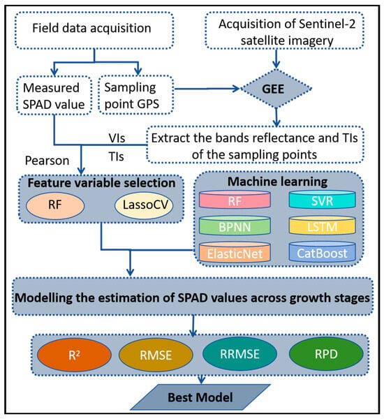
Figure 2.
Schematic diagram of the optimal model’s development.
In this research, the dataset of Huaisi Town was split into a training dataset and a testing dataset, adhering to a ratio of 8:2, through a randomized division process. In order to enhance the model’s performance and prevent overfitting, a K-fold CV approach (K = 5) was utilized during the training phase (with a sample size of 167). The models’ performance was subsequently assessed using the separate testing dataset that was not utilized during the model’s development process.
To rigorously evaluate the spatiotemporal transferability of the optimal model developed from the Huaisi Town training dataset, this research employed the Touqiao Town sub-study area dataset as an independent validation set. Notably, these two sub-study areas exhibited distinct agricultural phenological characteristics, particularly in sowing dates. Furthermore, the Touqiao Town dataset encompassed the critical jointing growth stage, a phenological phase absent in the Huaisi Town dataset. These substantive differences significantly strengthen the robustness of our validation approach for assessing the model’s spatiotemporal transferability within the region.
2.6. Model Performance Evaluation Metrics
For the evaluation of the model’s accuracy, our focus was directed toward four pivotal metrics: the Coefficient of Determination (R2, explicated in Equation (1)), Root Mean Square Error (RMSE, explicated in Equation (2)), Relative RMSE (RRMSE, explicated in Equation (3)), and the Ratio of Percentage Deviation (RPD, explicated in Equation (4)). Ordinarily, a higher R2 value, complemented by lower RMSE and RRMSE values, signifies an enhanced model performance. When interpreting RPD values in the article by Viscarra Rossel et al. [64], a value below 1.4 indicates very poor or poor estimations, 1.4 ≤ RPD < 1.8 suggests fair estimations, 1.8 ≤ RPD < 2.0 signifies good estimations, 2.0 ≤ RPD < 2.5 points to very good estimations, and RPD ≥ 2.5 denotes excellent estimations.
where is the measured SPAD value of sample i; is the estimated SPAD value of sample ; is the mean SPAD value; and is the number of samples. is the standard deviation between the estimated and measured SPAD values.
3. Results
3.1. Statistical Analysis of Measured SPAD Values
Table 3 presents comprehensive observations of winter wheat SPAD values at various growth stages in the two sub-study areas of Huaisi Town and Touqiao Town. Notably, the cumulative SPAD value analysis across all growth stages in Huaisi Town yielded a coefficient of variation (C·V) of 17.41%, emphasizing temporal heterogeneity. According to Kahaer and Tashpolat [65], a C·V < 15% indicates a slight variation, while 15% < C·V < 36% denotes a moderate variation. A higher C·V is beneficial for the following development of models, as it signifies improved applicability and robustness.
Table 3.
Evaluation of the measured SPAD value data division results.
3.2. Variable Selection
A two-step approach was adopted, initially utilizing RF for variable selection followed by LassoCV, to identify the optimal combination of RS variables for subsequent modeling. The RF variable selection process revealed that the RF method appeared to have limitations in effectively discerning the optimal variables for further modeling. The RF variable selection curve (Figure 3) serves to identify the minimum number of variables that provide optimal modeling capability (determined through 5-fold CV). The set of variables corresponding to the minimum RMSE represents the optimal variables. Within the set of VIs, a total of 18 variables were identified as optimal. In the case of the TI variable set, a total of 57 variables were identified as optimal. Furthermore, in the VI+TI variable set, a total of 92 variables were identified as optimal. Relying solely on RF variable selection in this research fails to effectively identify the most critical variables or substantially reduce the variable count.
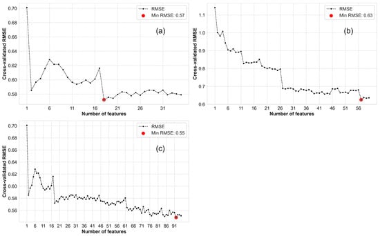
Figure 3.
RF variable selection curve. (a) VIs; (b) TIs; and (c) VIs+TIs.
After performing RF variable selection, LassoCV was further employed for variable selection, aiming to refine the variable set by penalizing the absolute size of the regression coefficients (alpha = 0.01). This approach is anticipated to yield a more streamlined and potentially more effective set of variables for estimation modeling.
Through LassoCV variable selection (Figure 4), it was observed that a more concise and crucial set of optimal variables was identified, building upon the RF variable selection. Within the variable set of VIs, a total of 10 variables were identified as optimal. In the case of the TI variable set, a total of 23 variables were identified as optimal. Furthermore, in the VI+TI variable set, a total of 26 variables were identified as optimal. As anticipated, the two-step variable selection process (RF-LassoCV) can markedly reduce the variable set without compromising the model’s accuracy, and even enhance the model’s performance.
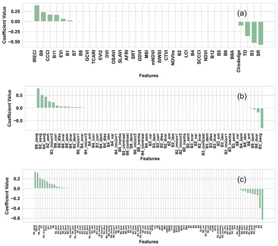
Figure 4.
Variable importance ranking from LassoCV variable selection. (a) VIs; (b) TIs; and (c) VIs+TIs.
Table 4 presents the specific optimal variables in different optimal variable sets (including VIs, TIs, and VIs+TIs) after RF-Lasso variable selection. These optimal variables will be utilized as inputs for subsequent machine learning algorithms to develop a superior estimation model for estimating winter wheat SPAD values. This carefully curated set of variables will contribute to improving the estimation accuracy and interpretability of the model, providing accurate estimates of winter wheat growth status.
Table 4.
Optimal variables used for subsequent modeling.
3.3. Model Development and Evaluation
In this research, nine machine learning algorithms, specifically SVR with various kernels (SVR-RBF, SVR-Poly, SVR-Sigmoid, and SVR-Linear), RF, CatBoost, BPNN, LSTM, and ElasticNet, were utilized to estimate SPAD values throughout the entire growth cycle of winter wheat in the sub-study area of Huaisi Town. These machine learning algorithms were applied using different combinations of variables, including VIs and TIs, and incorporating VIs and TIs, refined through RF and LassoCV variable selection.
To optimize the parameters and hyperparameters of the various machine learning algorithms employed in this study, a 5-fold CV combined with grid search was utilized on the training dataset. Table 5 presents the accuracy of different winter wheat SPAD value estimation models on the training dataset (via CV) using various combinations of variables. Each winter wheat SPAD value estimation model was developed using the optimized parameters and hyperparameters, as detailed in Table A3 in Appendix A. The performance of these models was further validated on the training dataset (non-CV) and testing dataset (Table 6).
Table 5.
Accuracy of SPAD value estimation models (Train (CV)) in Huaisi Town.
Table 6.
Accuracy of SPAD value estimation models in Huaisi Town.
Regarding the VI variable set, the SVR-Linear model (SVR-LinearVIs) demonstrates outstanding estimation performance, with an R2 of 0.7311, RMSE of 3.8778, RRMSE of 0.0852, and RPD of 1.9531 on the test dataset. In terms of the TI variable set, the SVR-RBF model (SVR-RBFTIs) achieves optimal accuracy, with an R2 of 0.7608, RMSE of 3.6578, RRMSE of 0.0804, and RPD of 2.0706 on the test dataset. In comparison to the SVR-LinearVIs model, this model demonstrated a 4.06% improvement in R2 and a 5.67% reduction in RMSE. The model exhibited commendable performance when modeling with the TI variable set, effectively capturing the dynamic information of SPAD values in winter wheat, thereby enhancing the accuracy of SPAD value estimation.
Furthermore, in the case of the VI+TI variable set, SVR-RBF similarly achieves optimal accuracy, with an R2 of 0.8131, RMSE of 3.2333, RRMSE of 0.0710, and RPD of 2.3424 on the test dataset. In comparison to the SVR-LinearVIs model, this model demonstrated an 11.22% improvement in R2 and a 16.627% reduction in RMSE. The VI+TI variable set improved the overall accuracy across all models. This promotion further highlights the capability of utilizing multisource data to improve the model’s estimation performance for SPAD values, more comprehensively and accurately reflecting the SPAD values in winter wheat.
Particularly noteworthy is the SVR-RBFVIs+TIs model, which achieved the highest R2 and RPD, as well as the lowest RMSE and RRMSE on the test set. This performance underscores SVR-RBFVIs+TIs as the optimal cross-growth-stage model capable of estimating SPAD values throughout the entire growth cycle of winter wheat in field environments.
For a more in-depth analysis of modeling accuracy, Figure 5 showcases scatter plots comparing the measured SPAD values with those estimated by the top-performing models across the three variable sets (Table 6). The majority of data points in the figure concentrate around the 1:1 diagonal line, signifying the solid agreement between measured and estimated values. This alignment highlights the models’ capability to span diverse growth stages and provide accurate estimations of SPAD values in wheat with minimal discrepancies.
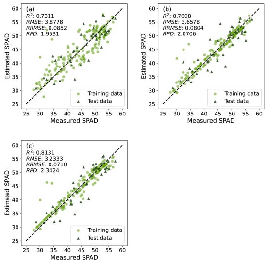
Figure 5.
Scatter plots of the optimal models for different variable sets in Huaisi Town. (a) SVR-LinearVIs; (b) SVR-RBFTIs; and (c) SVR-RBFVIs+TIs. Table A3 details the optimal parameter combinations for all models in the scatter plots and the corresponding training dataset accuracies.
3.4. Reliability Verification of the Optimal Model (SVR-RBFVIs+TIs)
3.4.1. SHAP Analysis of the Optimal Model
In this study, SHAP values were utilized to further analyze the importance and contribution of variables in the optimal estimation model (SVR-RBFVIs+TIs) that was developed based on the Huaisi Town training dataset. Figure 6 integrates variable importance and effect plots, displaying the distribution of SHAP values for the top 20 variables ranked by their influence on the model’s estimation. This visualization aids in understanding the contribution of these variables to the model’s estimation accuracy. Variables at the top of the figure (e.g., TO, B3, CCCI, B11, B9, B3_savg, B4_asm, and B3_imcorr2) exhibit a substantial range of positive (represented by red dots) and negative (represented by blue dots) impacts, indicating significant variability in their effects on model estimations for different SPAD values. Middle-tier variables (e.g., B1, B8_sent, B8_savg, B3_diss, B8_dent, B3_imcorr1, and CIrededge) also show both colors, but with more concentrated distributions, suggesting a relatively smaller impact on model estimations. Variables at the bottom (e.g., EVI, B2_corr, SR, B8_svar, and B4_dent) have the least impact on the model, with most effects close to zero, indicating minimal contribution to model estimations. Overall, both VIs and TIs substantially contribute to the optimal model’s estimation performance. This finding aligns with the observation that incorporating multimodal data consistently enhances the robustness of estimations for winter wheat SPAD values.
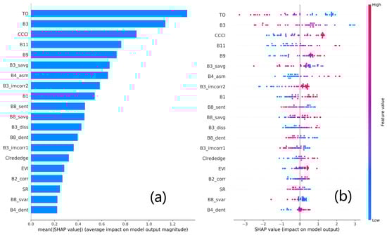
Figure 6.
SHAP summary plot for variable importance and impact on SPAD value estimation. (a) Variables are ranked vertically according to their impact, from top to bottom; (b) Red points indicate that the variable values have a positive impact on the model’s estimation for this observation, while blue points indicate a negative impact. The further a point is from the central line (zero), the greater the variable’s impact on the model’s estimation (positive SHAP values indicate a positive impact, and negative SHAP values indicate a negative impact).
3.4.2. Performance Evaluation of the Optimal Model for Winter Wheat with Different Sowing Times in Huaisi Town
This research employed the optimal model (SVR-RBFVIs+TIs) to validate the SPAD values of field plots at three different sowing times (normal, intermediate, and late) within the testing dataset. These sowing times were determined based on on-site observations. Table 7 shows that the SVR-RBFVIs+TIs model demonstrates favorable performance in estimating SPAD values for different sowing times. The model performs best in the normal sowing time, but also satisfactorily in the intermediate and late sowing time. Additionally, the scatter plot (Figure 7) depicting the measured SPAD values versus estimated SPAD values (test) for winter wheat in different sowing times further illustrates that the optimal model effectively estimates SPAD values across various sowing times.
Table 7.
Performance of the optimal model for winter wheat with different sowing dates in Huaisi Town.
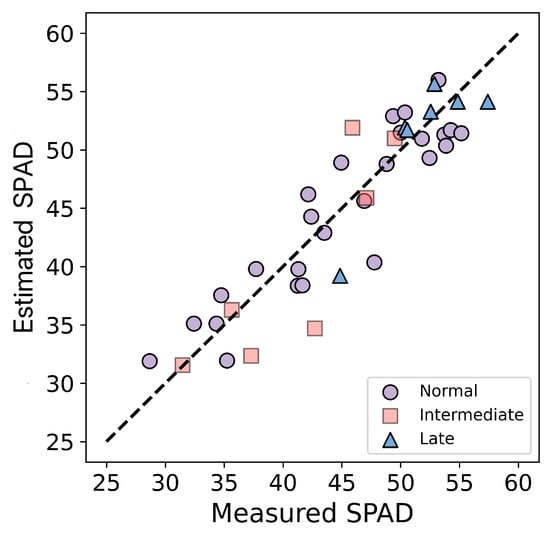
Figure 7.
Scatter plot of the optimal model at different sowing times in Huaisi Town.
3.4.3. The Optimal Model’s Transferability in Touqiao Town
This research evaluated the regional transferability of the optimal cross-growth-stage winter wheat SPAD value estimation model (SVR-RBFVIs+TIs) by applying it, originally developed from the Huaisi Town training dataset, to Touqiao Town, where sowing times differ significantly.
As presented in Figure 8 and Table 8, the results demonstrate that during the jointing stage, the model achieved an R2 of 0.7091, RMSE of 1.8096, and RRMSE of 0.0379. During the grain-filling stage, the model achieved an R2 of 0.6332, RMSE of 4.0287, and RRMSE of 0.0829. Overall, across both growth stages, the model exhibited an R2 of 0.6504, RMSE of 3.1348, and RRMSE of 0.0650. These results indicate that the model possesses favorable transferability in the local region, showcasing its ability to effectively estimate SPAD values in different growth stages and geographical locations.
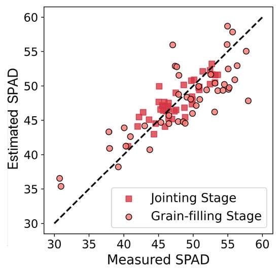
Figure 8.
Verification of scatter plots of the optimal model’s transferability in Touqiao Town.
Table 8.
Validation of the optimal model’s transferability in Touqiao Town.
3.5. Impact of the Training Dataset Size on Accuracy
To assess the sensitivity of various machine learning algorithms to different training dataset sample sizes, the training dataset sample sizes were adjusted to 67, 87, 107, 127, 147, and 167 for modeling purposes (including ModelVIs, ModelTIs, and ModelVIs+TIs). The performance of different machine learning algorithms improves as more data are added to the training dataset (Figure 9). Algorithms that exhibit a solid response to adding data include SVR-RBF, SVR-Poly, SVR-Linear, CatBoost, RF, BPNN, LSTM, and ElasticNet. Only SVR-Sigmoid does not show stable performance improvement, highlighting its limited suitability for estimating winter wheat SPAD values. SVR-RBF maintains a consistently high ranking across different training dataset sizes. Additionally, although most machine learning algorithms appear to approach saturation, they may still benefit from even more significant amounts of data to achieve higher accuracy.
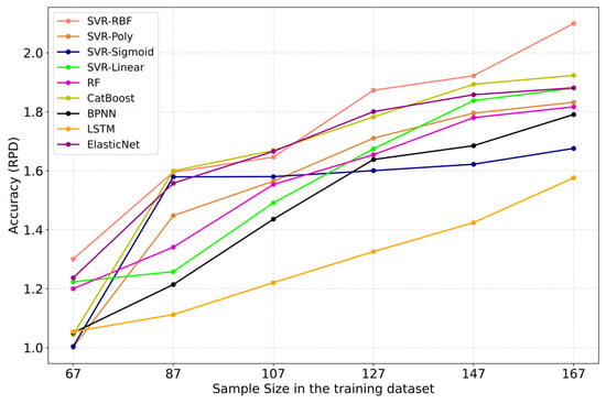
Figure 9.
Impact of training dataset size on machine learning algorithms’ performance. To maintain consistency, 5-fold CV was employed during the training phase, followed by testing using the test dataset to evaluate the performance of each machine learning algorithm under varying training dataset sample sizes based on the obtained RPD values (the mean RPD values obtained for ModelVIs, ModelTIs, and ModelVIs+TIs represent the RPD value for each respective machine learning algorithm). Ranking of different machine learning algorithms based on RPD values.
4. Discussion
4.1. The Optimal Model’s Stability and Transferability in the Region
The newly developed optimal model SVR-RBFVIs+TIs for estimating the SPAD values of winter wheat throughout its growth cycle in the region with multiple sowing dates, incorporating VIs and TIs and refined through RF-LassoCV variable selections, utilizing SVR-RBF, has demonstrated superior performance. This model achieved an RPD value of 2.3424, exceeding the threshold of 2.0. According to Viscarra Rossel et al. [64], this performance indicates exceptionally good estimation capabilities for estimating the SPAD values of winter wheat throughout its growth cycle. Furthermore, with the highest R2 value and the lowest RMSE and RRMSE, this model provides a robust framework for estimating the SPAD values of winter wheat throughout its growth cycle, making it the most outstanding model in the region with multiple sowing dates.
In most research on cereal crops, significant differences in SPAD values at different growth stages have been noted [66]. Additionally, variety and environmental factors (such as soil type, water, and nutrient management, etc.) are significant sources of variation in wheat SPAD values [67,68]. Therefore, the newly developed optimal model’s transferability in the local region was validated in an ‘unknown’ area outside the model’s spatial domain. The area differs in environmental conditions, winter wheat varieties, and sowing times compared to the optimal model’s spatial domain (specific differences are detailed in Section 2.1 (Study Area)). Furthermore, the independent validation dataset includes a growth stage (tillering stage) not covered by the model, which enhances the reliable validation of the optimal model’s transferability in the local region. Therefore, the developed optimal cross-growth-stage model (SVR-RBFVIs+TIs), calibrated based on SPAD values under different genotypes and environmental conditions, holds promise for application in other crops or under various environmental conditions in the future.
4.2. Impacts of Different Variable Sets on SPAD Value Estimation
Through RF-LassoCV variable selections, various optimal variable sets were generated, minimizing the impact of redundancy and collinearity among the selected variables on subsequent machine learning modeling. As anticipated, the general trend in the estimation performance of the six machine learning algorithms using various optimal variable sets is as follows: VIs+TIs > TIs > VIs.
As reported in previous studies, VIs and other spectral information have become the most commonly used RS indicators in crop parameter monitoring due to their stability and superior performance [59,69]. VIs provide spectral information about the winter wheat canopy. During the development of the SPAD value estimation model for winter wheat in the local region with multiple sowing dates, acceptable estimation outcomes were achieved (optimal model SVR-LinearVIs: R2 = 0.7311, RMSE = 3.8778, RRMSE = 0.0852, and RPD = 1.9531).
It is encouraging to note that this study found that modeling using only TIs extracted from Sentinel-2 MSI’s B2, B3, B4, and B8 bands (with a resolution of 10 m) also demonstrated superior estimation results compared to VIs (optimal model SVR-RBFTIs: R2 = 0.7608, RMSE = 3.6578, RRMSE = 0.0804, and RPD = 2.0706). Results indicate that the TI variable set is a promising alternative to the commonly used VI variable set, particularly for multi-temporal data [70]. This preference may be attributed to the evident variations in the winter wheat canopy structure of fields with different SPAD values observed through satellite images [49,71], significantly contributing to the development of the winter wheat SPAD value estimation model. As described in the study of Colombo et al. [72], TIs were able to show the spatial patterns of crop, shadow, and soil pixels.
Furthermore, many studies based on higher-resolution UAV RS images have reported the potential of incorporating VIs and TIs in monitoring other crop parameters (e.g., nitrogen concentration, yield) [71]. Distinct from previous work, the TIs employed in this study were derived from satellite imagery rather than UAV-based data. In this research, the optimal winter wheat SPAD value estimation model, developed by incorporating VIs and TIs extracted from satellite RS images (SVR-RBFVIs+TIs), significantly improved estimation accuracy, irrespective of the machine learning algorithm employed. Incorporating multimodal data consistently provided outstanding performance for the estimation model of winter wheat SPAD values across growth stages.
To date, no studies have been identified that apply satellite-derived TIs for agricultural parameter estimation. In the field of soil RS, only Wang et al. (2025) [73] have recently pioneered the extraction of TIs from different spectral bands of Sentinel-2 MSI (Level-2A) imagery—the same data source adopted in this study—and demonstrated that the integration of spectral and texture information is essential for accurately estimating soil organic carbon content (SOCC). Their findings further underscore the significance of texture information contained in satellite imagery.
While the 10 m resolution of Sentinel-2 MSI imagery is indeed coarser than the scale of individual wheat plants, each pixel still captures aggregate canopy-level variability arising from within-field heterogeneity. Factors such as non-uniform soil nutrient content, slight topographic variations, irrigation patterns, and microclimatic differences result in spatial differences in crop growth, leaf density, and chlorophyll content—even in seemingly homogeneous fields [71,73]. These variations manifest as subtle differences in reflectance and spatial texture on the plot scale.
4.3. VIs and TIs in the Optimal Model (SVR-RBFVIs+TIs)
Based on the SHAP analysis of the optimal model (SVR-RBFVIs+TIs), this study identified several key variables contributing significantly to the estimation of winter wheat SPAD values. The analysis revealed that specific single bands B1, B3, B9, and B11, as well as VIs (such as TO, CCCI, EVI, and SR), contribute significantly to the estimation of winter wheat SPAD values. It is worth noting that the single bands B9 and B11, which contribute significantly to winter wheat SPAD values, both belong to the short-wave infrared (SWIR) region. SWIR wavelengths possess important characteristics associated with nutrients and overall plant physiology, consistent with previous research findings [28]. Additionally, CCCI, EVI, and SR all incorporate two spectral bands, B4 (R, 650–680 nm) and B8 (NIR, 785–900 nm). This principle also parallels the design of the SPAD-502Plus meter, which utilizes two light-emitting diodes (at 650 and 940 nm) and a photodiode detector to measure the transmission of R and NIR light through leaves sequentially [74,75]. The addition of the Rededge (B5, B6, and B7) further enhances the responsiveness of these VIs to winter wheat SPAD values [76].
Existing studies that incorporate TIs to improve crop parameter estimation often lack direct evidence of observable textural variations, even though their objective results underscore the importance of TIs [77]. Some research has attempted to explore the associations between TIs and target variables. For instance, Meng et al. [77] reported that within GLCM-derived TIs, variance and contrast exhibited the strongest correlations with organ biomass, as these two metrics quantify local and global heterogeneity, respectively. Similarly, Yan et al. [78] found that TIs such as R-mean, B-mean, R-diss, R-contrast, G-mean, and R-var were well correlated with SPAD values in pear leaves, whereas TIs derived from the red-edge bands showed relatively poor performance in estimating SPAD values. This finding is largely consistent with the results of this study, in which the optimal GLCM-based TIs—specifically B3_savg, B4_asm, and B3_imcorr2—contributed most significantly to the estimation of winter wheat SPAD values. Specifically, B3_savg reflects the overall brightness and average reflectance level of the winter wheat canopy surfaces captured in Band 3, while B4_asm characterizes the uniformity and regularity of grayscale levels in Band 4, indicating the textural homogeneity of canopy surfaces. Additionally, B3_imcorr2 measures the linear dependency and correlation between pixel pairs at a specified distance in Band 3, providing insights into the spatial structure and arrangement of grayscale levels within the canopy. Changes in structural variables may reflect the growth environment, nutrient status, and physiological condition, which in turn influence the synthesis and content of chlorophyll [22].
4.4. Limitations and Future Research
The optimal model developed in this research was only validated within the local region, so its transferability to other regions requires more sample data across larger areas. Collecting additional data will help optimize the transferability of the winter wheat cross-growth-stage SPAD value estimation model developed in this research, which will be a primary focus of our future research.
Furthermore, it is essential to note that this research only covers data collected within one year. The conclusions drawn from the research should be further validated in future studies. This will contribute to ensuring the model’s robustness and reliability, making it better suited for practical applications in different years and environmental conditions.
5. Conclusions
By utilizing multi-temporal Sentinel-2 satellite imagery, this research developed a robust model (i.e., SVR-RBFVIs+TIs) for estimating winter wheat SPAD values spanning diverse growth stages (from tillering to grain-filling). The model also exhibited good applicability across different sowing times of winter wheat. Furthermore, the model exhibited favorable estimation accuracy at the other sub-study area with different sowing times, wheat varieties, and soil types from the modeling area. Particularly, the jointing stage of winter wheat that was included at the other sub-study area was not included for modeling. These results collectively indicated a demonstrable level of transferability for the estimation model across the region.
This study demonstrated that the incorporation of satellite-derived TIs significantly improved estimation model accuracy compared to the sole use of VIs typical in previous studies. The overall trend in modeling the winter wheat cross-growth-stage SPAD values using different optimal variable sets was as follows: VIs+TIs > TIs > VIs. This result suggested that despite the lower resolution of satellite imagery compared to UAV imagery, the TIs extracted from Sentinel-2 still held promise as a viable alternative to the commonly used VIs.
Author Contributions
J.C.: Formal analysis, Visualization, Writing—original draft, and Writing—review and editing. Q.Y.: Data curation, Formal analysis, Investigation, Methodology, Visualization, Writing—original draft, and Writing—review and editing. J.W.: Conceptualization, Formal analysis, Funding acquisition, Investigation, Methodology, Supervision, Writing—original draft, and Writing—review and editing. W.L.: Investigation and Visualization. Z.D.: Investigation. P.S.L.: Writing—review and editing. G.Z.: Supervision. Z.H.: Funding acquisition and Supervision. All authors have read and agreed to the published version of the manuscript.
Funding
This work was funded by the Scientific and Technological Innovation Fund of Carbon Emissions Peak and Neutrality of Jiangsu Provincial Department of Science and Technology [grant Number: BE2022424-2]; the Jiangsu Agricultural Science and Technology Innovation fund [grant Number: CX(22)1001]; the Science and Technology Program of Yangzhou City, Jiangsu, China [grant Number: YZ2021031]; and the Priority Academic Program Development of Jiangsu Higher Education Institutions (PAPD), China.
Data Availability Statement
The data are available from the authors upon reasonable request, as the data need further use.
Conflicts of Interest
The authors of this manuscript declare that there are no conflicts of interest.
Appendix A
Table A1.
Sentinel-2 spectral band information used in this study.
Table A1.
Sentinel-2 spectral band information used in this study.
| Band Code | Band Name | Sentinel-2A | Sentinel-2B | Resolution (m) | ||
|---|---|---|---|---|---|---|
| Central Wavelength (nm) | Bandwidth (nm) | Central Wavelength (nm) | Bandwidth (nm) | |||
| B1 | Coastal aerosol | 443.9 | 20 | 442.3 | 20 | 60 |
| B2 | Blue | 496.6 | 65 | 492.1 | 65 | 10 |
| B3 | Green | 560.0 | 35 | 559.0 | 35 | 10 |
| B4 | Red | 664.5 | 30 | 665.0 | 30 | 10 |
| B5 | Rededge | 703.9 | 15 | 703.8 | 15 | 20 |
| B6 | Rededge | 740.2 | 15 | 739.1 | 15 | 20 |
| B7 | Rededge | 782.5 | 20 | 779.7 | 20 | 20 |
| B8 | NIR | 835.1 | 115 | 833.0 | 115 | 10 |
| B8A | Narrow NIR | 864.8 | 20 | 864.0 | 20 | 20 |
| B9 | Water vapour | 945.0 | 20 | 943.2 | 20 | 60 |
| B11 | SWIR | 1613.7 | 90 | 1610.4 | 90 | 20 |
| B12 | SWIR | 2202.4 | 180 | 2185.7 | 180 | 20 |
Table A2.
The explanation of GLCM-TIs used in this research.
Table A2.
The explanation of GLCM-TIs used in this research.
| Abbreviation | Full Name | Explanation |
|---|---|---|
| asm | Angular Second Moment | Measures the uniformity of pixel values in an image. |
| corr | Correlation | Measures the linear dependency between pixel intensities at different locations. |
| dent | Difference Entropy | Measures the randomness or complexity of pixel value differences. |
| diss | Dissimilarity | Measures the average difference in pixel intensities between neighboring pixels. |
| dvar | Difference Variance | Measures the variance of pixel intensity differences. |
| ent | Entropy | Measures the randomness or uncertainty in pixel values. |
| idm | Inverse Difference Moment | Measures the local homogeneity of pixel values. |
| imcorr1, imcorr2 | Image Correlation 1 and 2 | Measures the correlation between different pixel pairs. |
| inertia | Inertia | Measures the local homogeneity of pixel values. |
| savg | Sum Average | Measures the distribution of local intensity sums in an image. |
| sent | Sum Entropy | Measures the randomness or complexity of pixel intensity sums. |
| svar | Sum Variance | Measures the variance of local intensity sums in an image. |
| var | Variance | Measures the variance of pixel intensities in an image. |
Table A3.
Accuracy of SVR models with different kernels and optimal parameters.
Table A3.
Accuracy of SVR models with different kernels and optimal parameters.
| Variable | Model | C | Epsilon |
|---|---|---|---|
| VIs | SVR-RBF | 17.48 | 1.00 |
| SVR-Poly | 7.65 | 0.42 | |
| SVR-Sigmoid | 0.91 | 0.01 | |
| SVR-Linear | 1.00 | 0.20 | |
| TIs | SVR-RBF | 29.27 | 1.00 |
| SVR-Poly | 15.27 | 4.48 | |
| SVR-Sigmoid | 1.27 | 0.01 | |
| SVR-Linear | 1.00 | 0.90 | |
| VIs+TIs | SVR-RBF | 19.94 | 1.00 |
| SVR-Poly | 17.05 | 0.46 | |
| SVR-Sigmoid | 1.03 | 0.01 | |
| SVR-Linear | 0.60 | 0.60 |
References
- Le Bail, M.; Jeuffroy, M.H.; Bouchard, C.; Barbottin, A. Is it possible to forecast the grain quality and yield of different varieties of winter wheat from Minolta SPAD meter measurements? Eur. J. Agron. 2005, 23, 379–391. [Google Scholar] [CrossRef]
- Yue, X.; Hu, Y.; Zhang, H.; Schmidhalter, U. Evaluation of both SPAD reading and SPAD index on estimating the plant nitrogen status of winter wheat. Int. J. Plant Prod. 2020, 14, 67–75. [Google Scholar] [CrossRef]
- Mehrabi, F.; Sepaskhah, A.R. Leaf nitrogen, based on SPAD chlorophyll reading can determine agronomic parameters of winter wheat. Int. J. Plant Prod. 2022, 16, 77–91. [Google Scholar] [CrossRef]
- Yang, X.; Yang, R.; Ye, Y.; Yuan, Z.; Wang, D.; Hua, K. Winter wheat SPAD estimation from UAV hyperspectral data using cluster-regression methods. Int. J. Appl. Earth Obs. Geoinf. 2021, 105, 102618. [Google Scholar] [CrossRef]
- Zhu, C.; Ding, J.; Zhang, Z.; Wang, J.; Wang, Z.; Chen, X.; Wang, J. SPAD monitoring of saline vegetation based on Gaussian mixture model and UAV hyperspectral image feature classification. Comput. Electron. Agric. 2022, 200, 107236. [Google Scholar] [CrossRef]
- Huang, Y.; Chen, Z.X.; Tao, Y.U.; Huang, X.Z.; Gu, X.F. Agricultural remote sensing big data: Management and applications. J. Integr. Agric. 2018, 17, 1915–1931. [Google Scholar] [CrossRef]
- Shao, J.; Zhao, W.; Zhou, Z.; Du, K.; Kong, L.; Wang, Y.A. new feasible method for yield gap analysis in regions dominanted by smallholder farmers, with a case study of Jiangsu Province, China. J. Integr. Agric. 2021, 20, 460–469. [Google Scholar] [CrossRef]
- Tian, Z.; Yin, Y.; Li, B.; Zhong, K.; Liu, X.; Jiang, D.; Cao, W.; Dai, T. Optimizing planting density and nitrogen application to mitigate yield loss and improve grain quality of late-sown wheat under rice-wheat rotation. J. Integr. Agric. 2024, 23, 2095–3119. [Google Scholar] [CrossRef]
- Shah, F.; Coulter, J.A.; Ye, C.; Wu, W. Yield penalty due to delayed sowing of winter wheat and the mitigatory role of increased seeding rate. Eur. J. Agron. 2020, 119, 126120. [Google Scholar] [CrossRef]
- Zhou, X.; Zhang, J.; Chen, D.; Huang, Y.; Kong, W.; Yuan, L.; Ye, H.; Huang, W. Assessment of leaf chlorophyll content models for winter wheat using Landsat-8 multispectral remote sensing data. Remote Sens. 2020, 12, 2574. [Google Scholar] [CrossRef]
- Wang, J.; Yin, Q.; Cao, L.; Zhang, Y.; Li, W.; Wang, W.; Zhou, G.; Huo, Z. Enhancing Winter Wheat Soil–Plant Analysis Development Value Prediction Through Evaluating Unmanned Aerial Vehicle Flight Altitudes, Predictor Variable Combinations, and Machine Learning Algorithms. Plants 2024, 13, 1926. [Google Scholar] [CrossRef] [PubMed]
- Chao, Z.; Liu, N.; Zhang, P.; Ying, T.; Song, K. Estimation methods developing with remote sensing information for energy crop biomass: A comparative review. Biomass Bioenergy 2019, 122, 414–425. [Google Scholar] [CrossRef]
- Hunter, F.D.L.; Mitchard, E.T.A.; Tyrrell, P.; Russell, S. Inter-Seasonal Time Series Imagery Enhances Classification Accuracy of Grazing Resource and Land Degradation Maps in a Savanna Ecosystem. Remote Sens. 2020, 12, 198. [Google Scholar] [CrossRef]
- Zhao, Y.; Meng, Y.; Han, S.; Feng, H.; Yang, G.; Li, Z. Should phenological information be applied to predict agronomic traits across growth stages of winter wheat? Crop. J. 2022, 10, 1346–1352. [Google Scholar] [CrossRef]
- Fu, H.; Chen, J.; Lu, J.; Yue, Y.; Xu, M.; Jiao, X.; Cui, G.; She, W. A Comparison of Different Remote Sensors for Ramie Leaf Area Index Estimation. Agronomy 2023, 13, 899. [Google Scholar] [CrossRef]
- Campos, I.; González-Gómez, L.; Villodre, J.; Calera, M.; Campoy, J.; Jiménez, N.; Plaza, C.L.; Sánchez-Prieto, S.; Calera, A. Mapping within-field variability in wheat yield and biomass using remote sensing vegetation indices. Precis. Agric. 2018, 20, 214–236. [Google Scholar] [CrossRef]
- Dhillon, M.S.; Dahms, T.; Kuebert-Flock, C.; Borg, E.; Conrad, C.; Ullmann, T. Modelling Crop Biomass from Synthetic Remote Sensing Time Series: Example for the DEMMIN Test Site, Germany. Remote Sens. 2020, 12, 1819. [Google Scholar] [CrossRef]
- Fu, Y.; Yang, G.; Wang, J.; Song, X.; Feng, H. Winter wheat biomass estimation based on spectral indices, band depth analysis and partial least squares regression using hyperspectral measurements. Comput. Electron. Agric. 2014, 100, 51–59. [Google Scholar] [CrossRef]
- Stroppiana, D.; Boschetti, M.; Brivio, P.A.; Bocchi, S. Plant nitrogen concentration in paddy rice from field canopy hyperspectral radiometry. Field Crops Res. 2009, 111, 119–129. [Google Scholar] [CrossRef]
- Zhou, K.; Cheng, T.; Zhu, Y.; Cao, W.; Ustin, S.L.; Zheng, H.; Yao, X.; Tian, Y. Assessing the impact of spatial resolution on the estimation of leaf nitrogen concentration over the full season of paddy rice using near-surface imaging spectroscopy data. Front. Plant Sci. 2018, 9, 964. [Google Scholar] [CrossRef] [PubMed]
- De Grandi, G.D.; Lucas, R.M.; Kropacek, J. Analysis by wavelet frames of spatial statistics in SAR data for characterizing structural properties of forests. IEEE Trans. Geosci. Remote Sens. 2008, 47, 494–507. [Google Scholar] [CrossRef]
- Guo, Y.; Xiao, Y.; Li, M.; Hao, F.; Zhang, X.; Sun, H.; Beurs, K.M.; Fu, Y.H.; He, Y. Identifying crop phenology using maize height constructed from multi-sources images. Int. J. Appl. Earth Obs. Geoinf. 2022, 115, 103121. [Google Scholar] [CrossRef]
- Zhu, L.; Hu, N.; Zhang, Z.; Xu, J.; Tao, B.; Meng, Y. Short-term responses of soil organic carbon and carbon pool management index to different annual straw return rates in a rice–wheat cropping system. Catena 2015, 135, 283–289. [Google Scholar] [CrossRef]
- Li, H.; Liu, L.; Wang, Z.; Yang, J.; Zhang, J. Agronomic and physiological performance of high-yielding wheat and rice in the lower reaches of Yangtze River of China. Field Crop Res. 2012, 133, 119–129. [Google Scholar] [CrossRef]
- Kandel, B.P. Spad value varies with age and leaf of maize plant and its relationship with grain yield. BMC Res. Notes 2020, 13, 475. [Google Scholar] [CrossRef] [PubMed]
- Liu, H.; Lei, X.; Liang, H.; Wang, X. Multi-Model Rice Canopy Chlorophyll Content Inversion Based on UAV Hyperspectral Images. Sustainability 2023, 15, 7038. [Google Scholar] [CrossRef]
- Kasampalis, D.; Alexandridis, T.K.; Deva, C.; Challinor, A.J.; Moshou, D.; Zalidis, G. Contribution of Remote Sensing on Crop Models: A Review. J. Imaging 2018, 4, 52. [Google Scholar] [CrossRef]
- Liu, N.; Townsend, P.A.; Naber, M.R.; Bethke, P.C.; Hills, W.B.; Wang, Y. Hyperspectral imagery to monitor crop nutrient status within and across growing seasons. Remote Sens. Environ. 2021, 255, 112303. [Google Scholar] [CrossRef]
- Prey, L.; Schmidhalter, U. Simulation of satellite reflectance data using high-frequency ground based hyperspectral canopy measurements for in-season estimation of grain yield and grain nitrogen status in winter wheat. ISPRS J. Photogramm. Remote Sens. 2019, 149, 176–187. [Google Scholar] [CrossRef]
- Sola Torralba, I.; García Martín, A.; Sandonís Pozo, L.; Álvarez-Mozos, J.; González de Audícana Amenábar, M. Assessment of atmospheric correction methods for Sentinel-2 images in Mediterranean landscapes. Int. J. Appl. Earth Obs. Geoinf. 2018, 73, 63–76. [Google Scholar]
- Li, J.; Roy, D.P. A global analysis of Sentinel-2A, Sentinel-2B and Landsat-8 data revisit intervals and implications for terrestrial monitoring. Remote Sens. 2017, 9, 902. [Google Scholar] [CrossRef]
- Carlson, T.N.; Ripley, D.A. On the relation between NDVI, fractional vegetation cover, and leaf area index. Remote Sens. Environ. 1997, 62, 241–252. [Google Scholar] [CrossRef]
- Barnes, E.M.; Clarke, T.; Richards, S.E.; Colaizzi, P.D.; Haberland, J.; Kostrzewski, M.; Waller, P.M.; Choi, C.Y.; Riley, E.; Thompson, T.L.; et al. Coincident detection of crop water stress, nitrogen status and canopy density using ground based multispectral data. In Proceedings of the Fifth International Conference on Precision Agriculture, Bloomington, MN, USA, 16–19 July 2000; p. 1619. [Google Scholar]
- Xie, Q.; Dash, J.; Huang, W.; Peng, D.; Qin, Q.; Mortimer, H.; Casa, R.; Pignatti, S.; Laneve, G.; Pascucci, S.; et al. Vegetation indices combining the red and red-edge spectral information for leaf area index retrieval. IEEE J. Sel. Top. Appl. Earth Obs. Remote Sens. 2018, 11, 1482–1493. [Google Scholar] [CrossRef]
- Frampton, W.J.; Dash, J.; Watmough, G.; Milton, E.J. Evaluating the capabilities of Sentinel-2 for quantitative estimation of biophysical variables in vegetation. ISPRS J. Photogramm. Remote Sens. 2013, 82, 83–92. [Google Scholar] [CrossRef]
- Datt, B. Remote sensing of water content in Eucalyptus leaves. Aust. J. Bot. 1999, 47, 909–923. [Google Scholar] [CrossRef]
- Gitelson, A.; Merzlyak, M.N. Quantitative estimation of chlorophyll-a using reflectance spectra: Experiments with autumn chestnut and maple leaves. J. Photochem. Photobiol. B Biol. 1994, 22, 247–252. [Google Scholar] [CrossRef]
- Perry, C.R., Jr.; Lautenschlager, L.F. Functional equivalence of spectral vegetation indices. Remote Sens. Environ. 1984, 14, 169–182. [Google Scholar] [CrossRef]
- Fensholt, R.; Sandholt, I. Derivation of a shortwave infrared water stress index from MODIS near-and shortwave infrared data in a semiarid environment. Remote Sens. Environ. 2003, 87, 111–121. [Google Scholar] [CrossRef]
- Huete, A.R.; Liu, H.Q.; Batchily, K.V.; Van Leeuwen, W.J.D.A. A comparison of vegetation indices over a global set of TM images for EOS-MODIS. Remote Sens. Environ. 1997, 59, 440–451. [Google Scholar] [CrossRef]
- Hunt, E.R., Jr.; Rock, B.N. Detection of changes in leaf water content using near- and middle-infrared reflectances. Remote Sens. Environ. 1989, 30, 43–54. [Google Scholar]
- Tucker, C.J.; Elgin, J.H., Jr.; McMurtrey, J.E., III; Fan, C.J. Monitoring corn and soybean crop development with hand-held radiometer spectral data. Remote Sens. Environ. 1979, 8, 237–248. [Google Scholar] [CrossRef]
- Karnieli, A.; Kaufman, Y.J.; Remer, L.; Wald, A. AFRI—Aerosol free vegetation index. Remote Sens. Environ. 2001, 77, 10–21. [Google Scholar] [CrossRef]
- Lymburner, L.; Beggs, P.J.; Jacobson, C.R. Estimation of canopy-average surface-specific leaf area using Landsat TM data. Photogramm. Eng. Remote Sens. 2000, 66, 183–192. [Google Scholar]
- Steven, M.D. The sensitivity of the OSAVI vegetation index to observational parameters. Remote Sens. Environ. 1998, 63, 49–60. [Google Scholar] [CrossRef]
- Jordan, C.F. Derivation of leaf-area index from quality of light on the forest floor. Ecology 1969, 50, 663–666. [Google Scholar] [CrossRef]
- Son, N.T.; Chen, C.F.; Chen, C.R.; Minh, V.Q.; Trung, N.H. A comparative analysis of multitemporal MODIS EVI and NDVI data for large-scale rice yield estimation. Agric. Meteorol. 2014, 197, 52–64. [Google Scholar] [CrossRef]
- Mondal, P. Quantifying surface gradients with a 2-band Enhanced Vegetation Index (EVI2). Ecol. Indic. 2011, 11, 918–924. [Google Scholar] [CrossRef]
- Haboudane, D.; Miller, J.R.; Tremblay, N.; Zarco-Tejada, P.J.; Dextraze, L. Integrated narrow-band vegetation indices for prediction of crop chlorophyll content for application to precision agriculture. Remote Sens. Environ. 2002, 81, 416–426. [Google Scholar] [CrossRef]
- Lobell, D.B.; Thau, D.; Seifert, C.; Engle, E.; Little, B. A scalable satellite-based crop yield mapper. Remote Sens. Environ. 2015, 164, 324–333. [Google Scholar] [CrossRef]
- Rondeaux, G.; Steven, M.; Baret, F. Optimization of soil-adjusted vegetation indices. Remote Sens. Environ. 1996, 55, 95–107. [Google Scholar] [CrossRef]
- Haralick, R.M.; Shanmugam, K.; Dinstein, I.H. Textural features for image classification. IEEE Trans. Syst. Man Cybern. 1973, 3, 610–621. [Google Scholar] [CrossRef]
- Hall-Beyer, M. Practical guidelines for choosing GLCM textures to use in landscape classification tasks over a range of moderate spatial scales. Int. J. Remote Sens. 2017, 38, 1312–1338. [Google Scholar] [CrossRef]
- Corrales, D.C.; Schoving, C.; Raynal, H.; Debaeke, P.; Journet, E.P.; Constantin, J. A surrogate model based on feature selection techniques and regression learners to improve soybean yield prediction in southern France. Comput. Electron. Agric. 2022, 192, 106578. [Google Scholar] [CrossRef]
- Ma, Z.; Li, W.; Warner, T.A.; He, C.; Wang, X.; Zhang, Y.; Guo, C.; Cheng, T.; Zhu, Y.; Cao, W.; et al. A framework combined stacking ensemble algorithm to classify crop in complex agricultural landscape of high altitude regions with Gaofen-6 imagery and elevation data. Int. J. Appl. Earth Obs. Geoinf. 2023, 122, 103386. [Google Scholar] [CrossRef]
- Darvishnezhad, M.A. multi-view ensemble model based on semi-supervised feature learning for small sample classification of PolSAR images. Int. J. Remote Sens. 2024, 45, 981–1031. [Google Scholar] [CrossRef]
- Liaw, A.; Wiener, M. Classification and regression by randomForest. R News 2002, 2, 18–22. [Google Scholar]
- García-Floriano, A.; López-Martín, C.; Yáñez-Márquez, C.; Abran, A. Support vector regression for predicting software enhancement effort. Inf. Softw. Technol. 2018, 97, 99–109. [Google Scholar] [CrossRef]
- Zhang, H.; Zhang, Y.; Liu, K.; Lan, S.; Gao, T.; Li, M. Winter wheat yield prediction using integrated Landsat 8 and Sentinel-2 vegetation index time-series data and machine learning algorithms. Comput. Electron. Agric. 2023, 213, 108250. [Google Scholar] [CrossRef]
- Heermann, P.D.; Khazenie, N. Classification of multispectral remote sensing data using a back-propagation neural network. IEEE Trans. Geosci. Remote Sens. 1992, 30, 81–88. [Google Scholar] [CrossRef]
- Sherstinsky, A. Fundamentals of recurrent neural network (RNN) and long short-term memory (LSTM) network. Phys. D Nonlinear Phenom. 2020, 404, 132306. [Google Scholar] [CrossRef]
- Zou, H.; Hastie, T. Regularization and variable selection via the elastic net. J. R. Stat. Soc. Ser. B 2005, 67, 301–320. [Google Scholar] [CrossRef]
- Lundberg, S.M.; Lee, S.I. A unified approach to interpreting model predictions. In Proceedings of the 31st International Conference on Neural Information Processing Systems (NIPS’17), Long Beach, CA, USA, 4–9 December 2017; Curran Associates Inc.: New York, NY, USA, 2017; pp. 4768–4777. [Google Scholar] [CrossRef]
- Viscarra Rossel, R.A.; Taylor, H.J.; McBratney, A.B. Multivariate calibration of hyperspectral γ-ray energy spectra for proximal soil sensing. Eur. J. Soil. Sci. 2007, 58, 343–353. [Google Scholar] [CrossRef]
- Kahaer, Y.; Tashpolat, N. Estimating salt concentrations based on optimized spectral indices in soils with regional heterogeneity. J. Spectrosc. 2019, 2019, 2402749. [Google Scholar] [CrossRef]
- Wang, G.; Bronson, K.F.; Thorp, K.R.; Mon, J.; Badaruddin, M. Multiple leaf measurements improve effectiveness of chlorophyll meter for durum wheat nitrogen management. Crop Sci. 2014, 54, 817–826. [Google Scholar] [CrossRef]
- Bavec, F.; Bavec, M. Chlorophyll meter readings of winter wheat cultivars and grain yield prediction. Commun. Soil Sci. Plant Anal. 2001, 32, 2709–2719. [Google Scholar] [CrossRef]
- Monostori, I.; Árendás, T.; Hoffman, B.; Galiba, G.; Gierczik, K.; Szira, F.; Vágújfalvi, A. Relationship between SPAD value and grain yield can be affected by cultivar, environment and soil nitrogen content in wheat. Euphytica 2016, 211, 103–112. [Google Scholar] [CrossRef]
- Segarra, J.; Araus, J.L.; Kefauver, S.C. Farming and Earth Observation: Sentinel-2 data to estimate within-field wheat grain yield. Int. J. Appl. Earth Obs. Geoinf. 2022, 107, 102697. [Google Scholar] [CrossRef]
- Maimaitijiang, M.; Sagan, V.; Sidike, P.; Hartling, S.; Esposito, F.; Fritschi, F.B. Soybean yield prediction from UAV using multimodal data fusion and deep learning. Remote Sens. Environ. 2020, 237, 111599. [Google Scholar] [CrossRef]
- Wang, Y.; Tan, S.; Jia, X.; Qi, L.; Liu, S.; Lu, H.; Wang, C.; Liu, W.; Zhao, X.; He, L.; et al. Estimating Relative Chlorophyll Content in Rice Leaves Using Unmanned Aerial Vehicle Multi-Spectral Images and Spectral–Textural Analysis. Agronomy 2023, 13, 1541. [Google Scholar] [CrossRef]
- Colombo, R.; Bellingeri, D.; Fasolini, D.; Marino, C.M. Retrieval of leaf area index in different vegetation types using high resolution satellite data. Remote Sens. Environ. 2003, 86, 120–131. [Google Scholar] [CrossRef]
- Wang, J.; Huang, J.; Zhang, Y.; Shang, J.; Yin, Q.; Li, W.; Cao, L.; Zhou, G.; Loh, P.S.; Dai, Q. Integration of Sentinel-1 and 2 for estimating soil organic carbon content in reclaimed coastal croplands with novel indices. Soil. Tillage Res. 2025, 252, 106629. [Google Scholar] [CrossRef]
- Atzberger, C.; Guérif, M.; Baret, F.; Werner, W. Comparative analysis of three chemometric techniques for the spectroradiometric assessment of canopy chlorophyll content in winter wheat. Comput. Electron. Agric. 2010, 73, 165–173. [Google Scholar] [CrossRef]
- Vincini, M.; Amaducci, S.; Frazzi, E. Empirical estimation of leaf chlorophyll density in winter wheat canopies using Sentinel-2 spectral resolution. IEEE Trans. Geosci. Remote Sens. 2013, 52, 3220–3235. [Google Scholar] [CrossRef]
- Li, D.; Cheng, T.; Zhou, K.; Zheng, H.; Yao, X.; Tian, Y.; Zhu, Y.; Cao, W. WREP: A wavelet-based technique for extracting the red edge position from reflectance spectra for estimating leaf and canopy chlorophyll contents of cereal crops. ISPRS J. Photogramm. Remote Sens. 2017, 129, 103–117. [Google Scholar] [CrossRef]
- Meng, L.; Ming, B.; Liu, Y.; Nie, C.; Fang, L.; Zhou, L.; Xin, J.; Xue, B.; Liang, Z.; Guo, H.; et al. Maize biomass estimation by integrating spectral, structural, and textural features from unmanned aerial vehicle data. Eur. J. Agron. 2025, 168, 127647. [Google Scholar] [CrossRef]
- Yan, N.; Qin, Y.; Wang, H.; Wang, Q.; Hu, F.; Wu, Y.; Zhang, X.; Li, X. The Inversion of SPAD Value in Pear Tree Leaves by Integrating Unmanned Aerial Vehicle Spectral Information and Textural Features. Sensors 2025, 25, 618. [Google Scholar] [CrossRef] [PubMed]
Disclaimer/Publisher’s Note: The statements, opinions and data contained in all publications are solely those of the individual author(s) and contributor(s) and not of MDPI and/or the editor(s). MDPI and/or the editor(s) disclaim responsibility for any injury to people or property resulting from any ideas, methods, instructions or products referred to in the content. |
© 2025 by the authors. Licensee MDPI, Basel, Switzerland. This article is an open access article distributed under the terms and conditions of the Creative Commons Attribution (CC BY) license (https://creativecommons.org/licenses/by/4.0/).