Flight Planning for LiDAR-Based UAS Mapping Applications

Abstract

In the last two decades, unmanned aircraft systems (UAS) were successfully used in different environments for diverse applications like territorial mapping, heritage 3D documentation, as built surveys, construction monitoring, solar panel placement and assessment, road inspections, etc. These applications were correlated to the onboard sensors like RGB cameras, multi-spectral cameras, thermal sensors, panoramic cameras, or LiDARs. According to the different onboard sensors, a different mission plan is required to satisfy the characteristics of the sensor and the project aims. For UAS LiDAR-based mapping missions, requirements for the flight planning are different with respect to conventional UAS image-based flight plans because of different reasons related to the LiDAR scanning mechanism, scanning range, output scanning rate, field of view (FOV), rotation speed, etc. Although flight planning for image-based UAS missions is a well-known and solved problem, flight planning for a LiDAR-based UAS mapping is still an open research topic that needs further investigations. The article presents the developments of a LiDAR-based UAS flight planning tool, tested with simulations in real scenarios. The flight planning simulations considered an UAS platform equipped, alternatively, with three low-cost multi-beam LiDARs, namely Quanergy M8, Velodyne VLP-16, and the Ouster OS-1-16. The specific characteristics of the three sensors were used to plan flights and acquired dense point clouds. Comparisons and analyses of the results showed clear relationships between point density, flying speeds, and flying heights.

1. Introduction

Flight planning is a solved problem since aerial photogrammetry started in the last century. Nowadays, flight planning is not restricted to the traditional aerial mapping missions but is also expanded to include unmanned aircraft system (UAS) mapping missions [1,2,3,4], which can be equipped with different sensors mounted on the UAS platform. Currently, there are many UAS flight planning tools, either free, commercial, or Webtools [5,6,7,8,9,10,11,12,13,14], which can be used prior to the mapping missions.

Generally, UAS flight planning for mapping missions can be divided into four types—(1) area-based, either on a grid or a polygon shape, (2) circular flights for high objects, (3) corridor flights for mapping railroads, railways, or powerlines, and (4) free mapping flights. Figure 1 illustrates the geometrical configuration of an image-based UAS flight plan where the necessary sidelap (cross-track) and endlap (along-track) percentages should be attained.

Furthermore, researchers keep working on the development of more advanced autonomous path planning techniques, which can be adopted for dynamic scenes like in disaster mapping applications and other autonomous robot-like tasks [15,16,17,18]. The basic idea is to find the optimal collision-free path of the UAS and its sensor pose in every view, by relying on the best next view (NBV) in an iterative way [15,19,20]. Furthermore, advanced scene understanding and SLAM techniques are also applied [18,21].

Similar to conventional camera-based missions, LiDAR sensors are widely used nowadays on board of UASs for different mapping applications like 3D modeling, land surveying, power line inspection, forestry, smart agriculture, mining, shallow water bathymetry, etc. [22,23,24,25]. It is worth mentioning that LiDAR sensors vary in their scanning mechanism as being spinning or solid state, multi or single beam, and in their range measurement principle, either by using time of flight TOF or the amplitude modulation of a continuous wave (AMCW) systems [26,27]. Special attention has been paid for the use of the low-cost multi-beam LiDARs for UAS mapping tasks because of their high productivity, level of accuracy, reasonable weights, and their low energy consumption [28,29,30,31,32].

Noticeably, flight planning for UAS LiDAR mapping systems is a new photogrammetric design problem, which is poorly explained in the literature and only few mapping companies were considered to build suitable software tools for their customers [33,34]. Some design parameters are common for both image-based and LiDAR-based UAS mapping missions, namely, flying speed, flying height, field of view (FOV), and the recommended overlap between images/strips. On the other hand, different design parameters are considered in the flight planning of the UAS LiDAR missions, like the maximum scanning range of the used LiDAR and the scanning rate.

Accordingly, and in the context of urban modeling and smart city technologies, three different low-cost multi-beam LiDAR sensors, namely Quanergy M8, Velodyne VLP-16, and the Ouster OS-1-16 [35,36,37], were used to simulate the acquisition of dense point clouds from a UAS platform.

In this article, we are trying to answer the following questions:

(1)

How to design a flight plan for mapping an area using a low-cost multi-beam LiDAR mounted on a UAS platform and what are the input and output parameters?

(2)

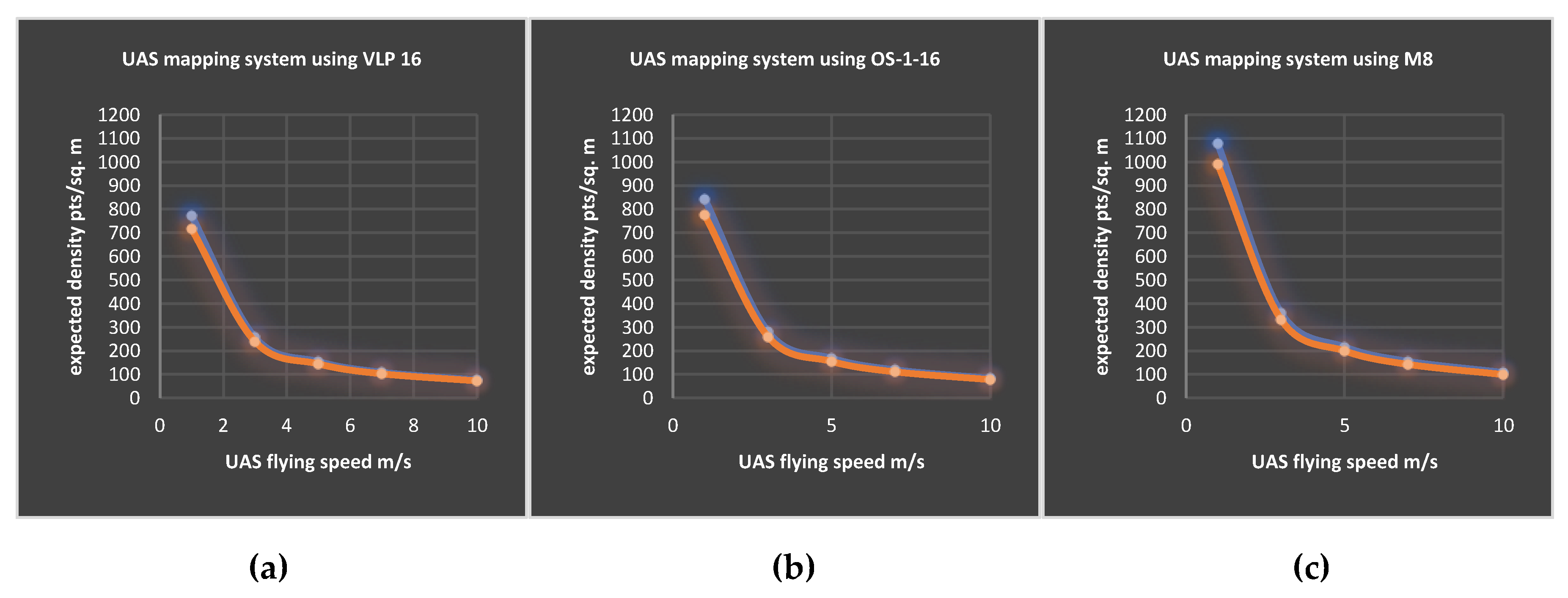
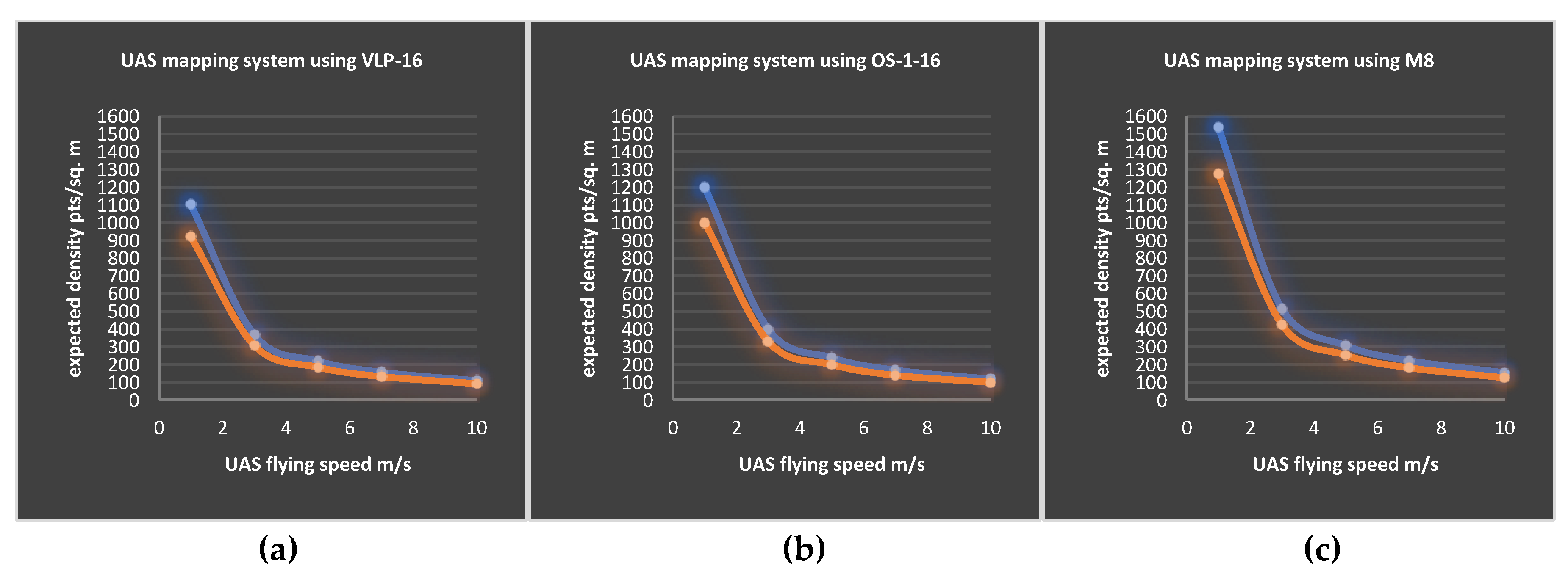
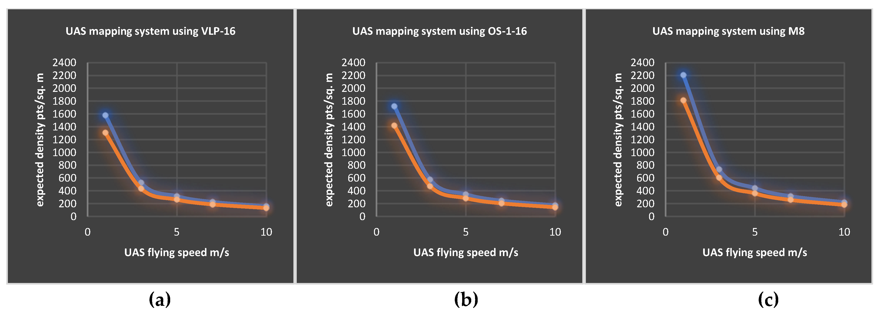
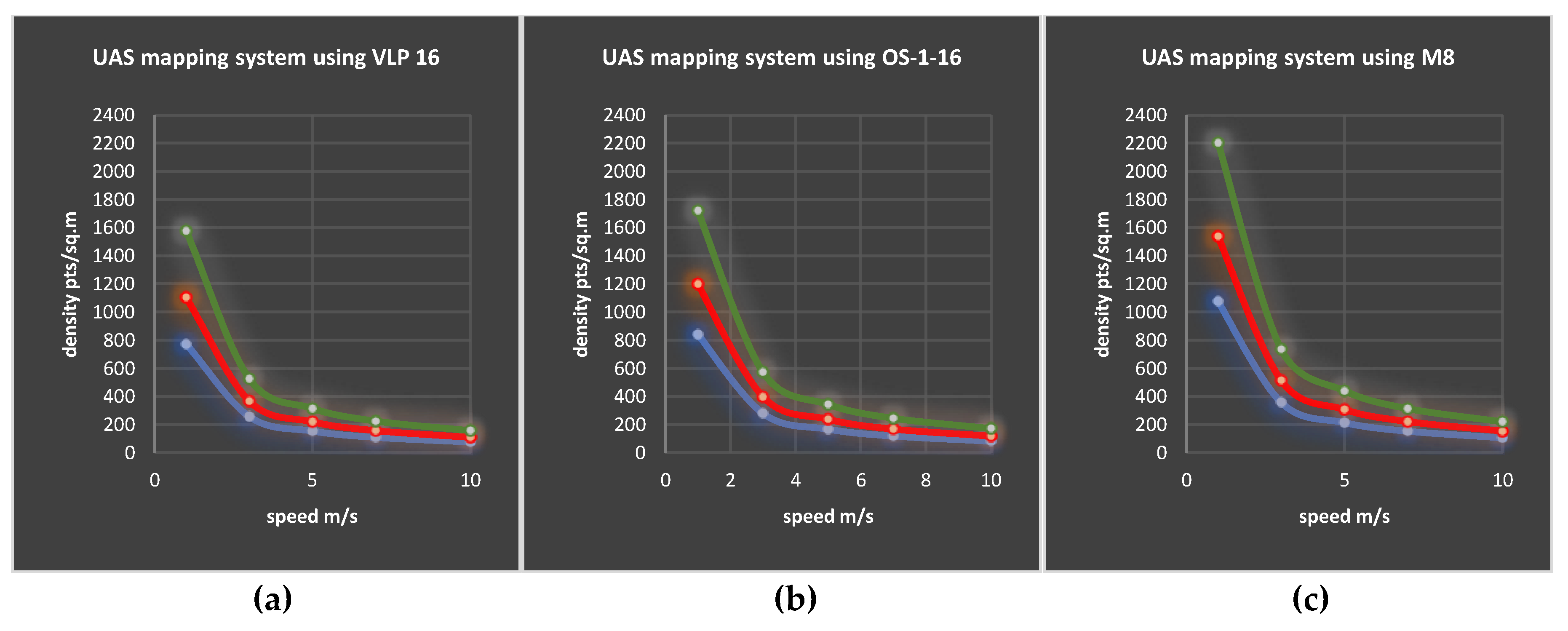
What is the expected point density in an urban region at different flying heights, sidelaps, and flying speeds using low-cost multi-beam LiDARs?

(3)

Among the considered low-cost LiDAR sensors, which one is more efficient for mapping purposes in terms of coverage and point density?

To answer these research questions, a clear methodology workflow is presented in Section 2 where the required design parameters and the necessary computations are well-defined. Furthermore, statistical graphics are given in Section 3.1 to clarify the relation between the flying height, speed, and the overlap percentages, using the mentioned low-cost multi-beam LiDARs. Finally, reality-like models of an urban region and a communication tower are scanned in two simulation experiments in Section 3.2 and Section 3.3, and the results are analyzed in terms of point density and coverage. Conclusions follow in Section 4.

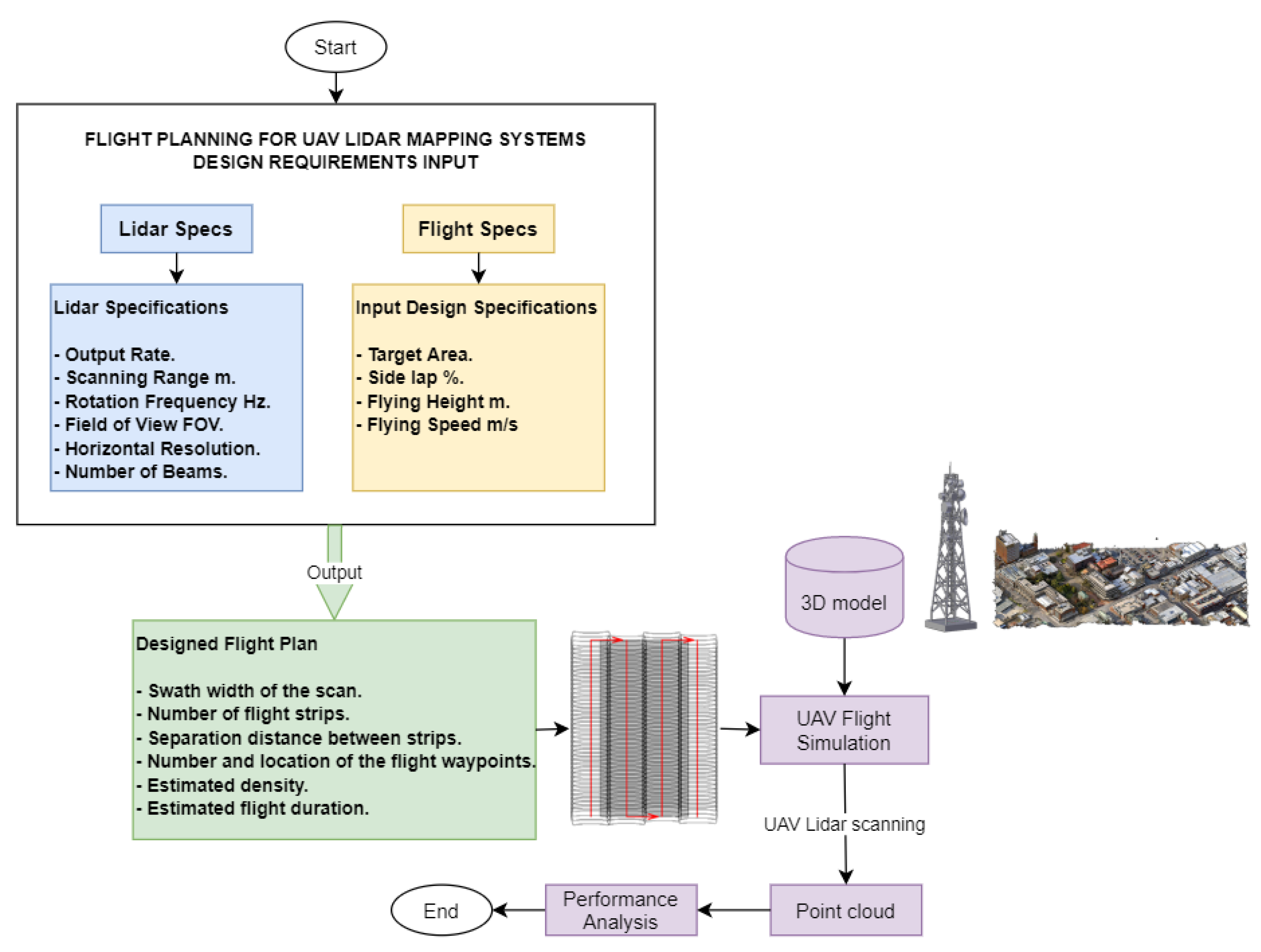
2. Methodology and Developed Tool

The developed methodology (Figure 2) consists of two parts—a flight planning tool part and some simulation tests on real-world scenarios. For every UAS LiDAR flight plan design, there are two types of input requirements—the LiDAR specifications and the flight specifications. LiDAR specifications, as mentioned earlier, include the scanning output rate, rotation speed, maximum scanning range, etc., while the mapping specifications are related to the shape and size of the target area, flight strips (lines) sidelap, flying height, and speed. The proposed methodology delivers the following output parameters:

• Swath width of the scan
• Number of flight strips
• Separation distance between flight strips
• Number and location of the flight waypoints
• Estimated point density
• Estimated flight duration

Given these output parameters, a 3D simulation is applied for testing the flight plan design tool and checking the validity of the estimated point density. Using the Blender tool [38], flight plans are simulated for mapping an urban environment (Section 3.3) [39] and a communication tower (Section 3.4). For these tests, we consider a UAS platform equipped three different types of low-cost multi-beam LiDARs, namely, Velodyne VLP-16, Quanergy M8, and Ouster OS-1-16 (

Table 1. Selected three low-cost LiDAR type specifications.

LiDAR Sensor/System	Velodyne [37]	Quanergy [35]	Ouster [36]
Type/version	VLP-16	M8	OS-1-16
Max. Range	≤ 100 m	> 100 m @ 80%	≤ 120 m @ 80%
Range Accuracy 1σ	±3 cm (Typical)	±3 cm	±1.5-10 cm
Output rate pts/sec.	≈300000	≈420000 (1 return)	≈327680
FOV - Vertical	≈30° (±15°)	≈20° (+3°/–17°)	≈33.2° (±16.6°)
Rotation rate	5-20 Hz	5-20 Hz	10-20 Hz
Vertical resolution	V:2°	V:3°	V: 2.2°
Horizontal resolution	H: 0.4°@ 20Hz	H: 0.14°@ 20Hz	H:0.35°@ 20Hz
Weight	830 g	900 g	425 g
Power consumption	8 w	18 w	14-20 w
Price	$8K	$5K	$3.5K

).

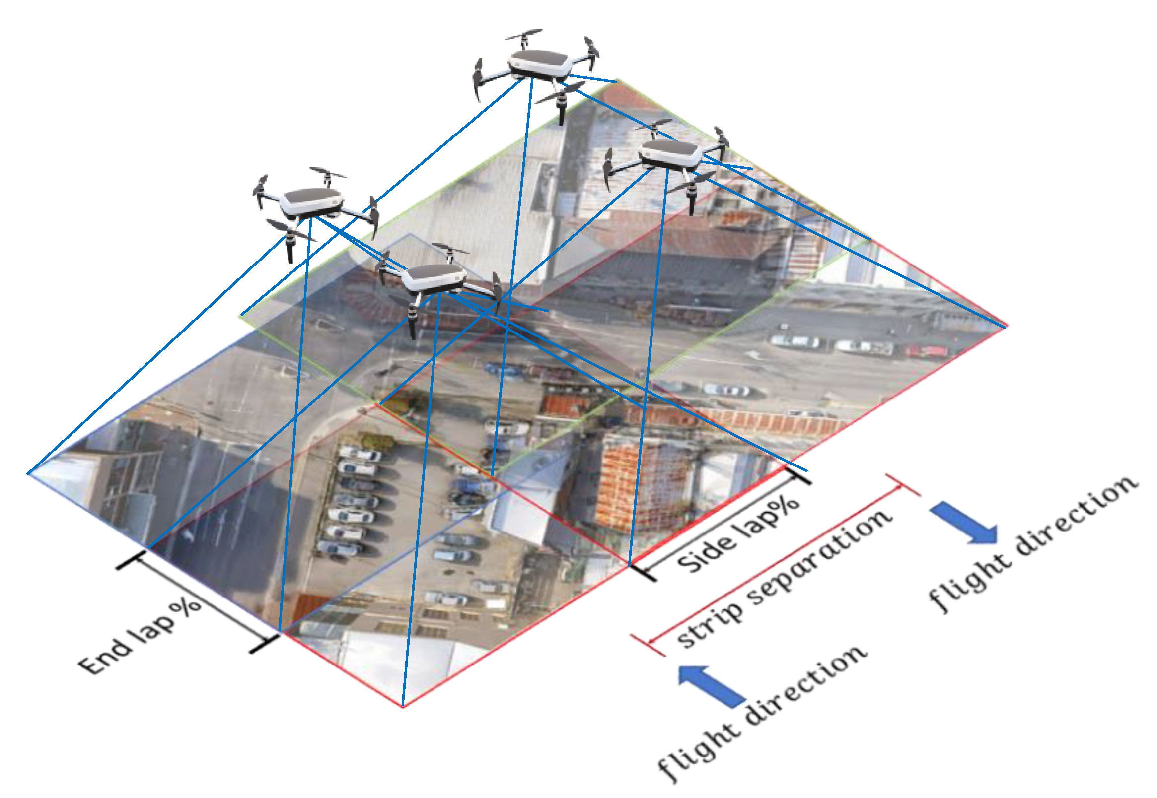
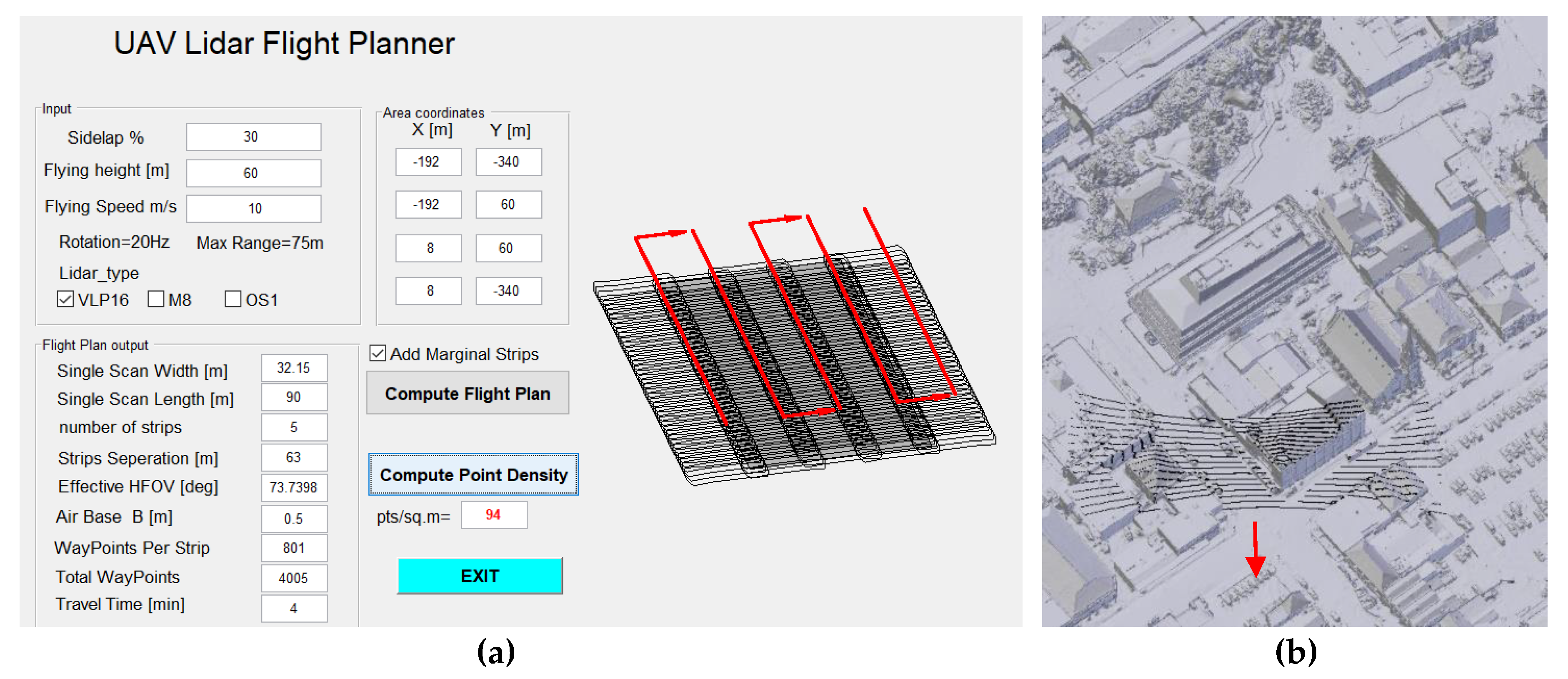
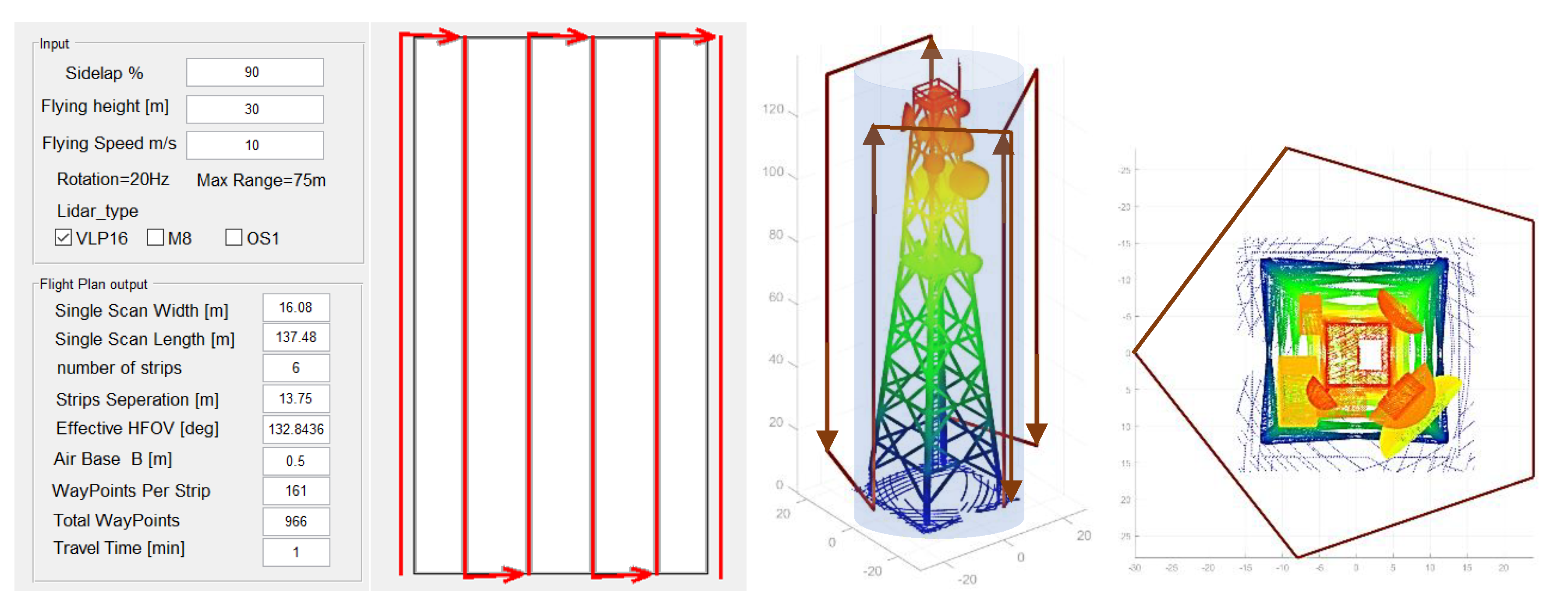
2.1. Flight Plan Design

The flight plan tool for a UAS LiDAR mapping system is realized as a standalone tool in MATLAB and it is available at https://github.com/Photogrammtery-Topics/UAV-Lidar-flight-planner. It should be noted that the proposed flight planning design is based on a LiDAR sensor mounted with a nadir orientation. Accordingly, for each multi-beam LiDAR sensors mounted onboard, we expect a specific footprint pattern of single scans on the ground that would be repeated while the UAS moved within time. On the other hand, flight parameters like the flying height and the overlap percentage between scans are required, to successfully design the flight plan. As shown in Figure 2, the required input parameters can be listed as follows:

• LiDAR specifications: Every multi-beam LiDAR sensor has its own geometric structure, which includes FOV, angular distribution of beams, angular resolution, output rate pts/m², rotation speed, and the maximum scanning range. Table 1 shows the characteristics of the three selected low-cost multi-beam LiDAR sensors, as published by their manufacturers [35,36,37].
• Flight plan specifications: They include flying height H, flying speed m/s, and the required sidelap % between adjacent scanning strips. It should be noted that a larger overlap percentage ensures higher coverage but requires a longer flight time, which should be carefully considered.

The mentioned flight plan parameters and the LiDAR specifications are used in the UAS LiDAR flight planning computations, as follows (Figure 3):

$$W=2 tan\left(\frac{VFOV}{2}\right)·H$$

(1)

$$L =2 \sqrt{\left(R^2-H^2\right)}$$

(2)

$$SFOV=2 ta{n}^{-1}\left(\frac{L/2}{H}\right)$$

(3)

$$SPD=\left(1-sidelap \%\right)·L$$

(4)

$$NFS=\frac{W_{area}}{SPD}+1$$

(5)

$$NScan=\frac{L_{area}}{B}+1$$

(6)

$$Total waypoints=NFS\times NScan$$

(7)

where

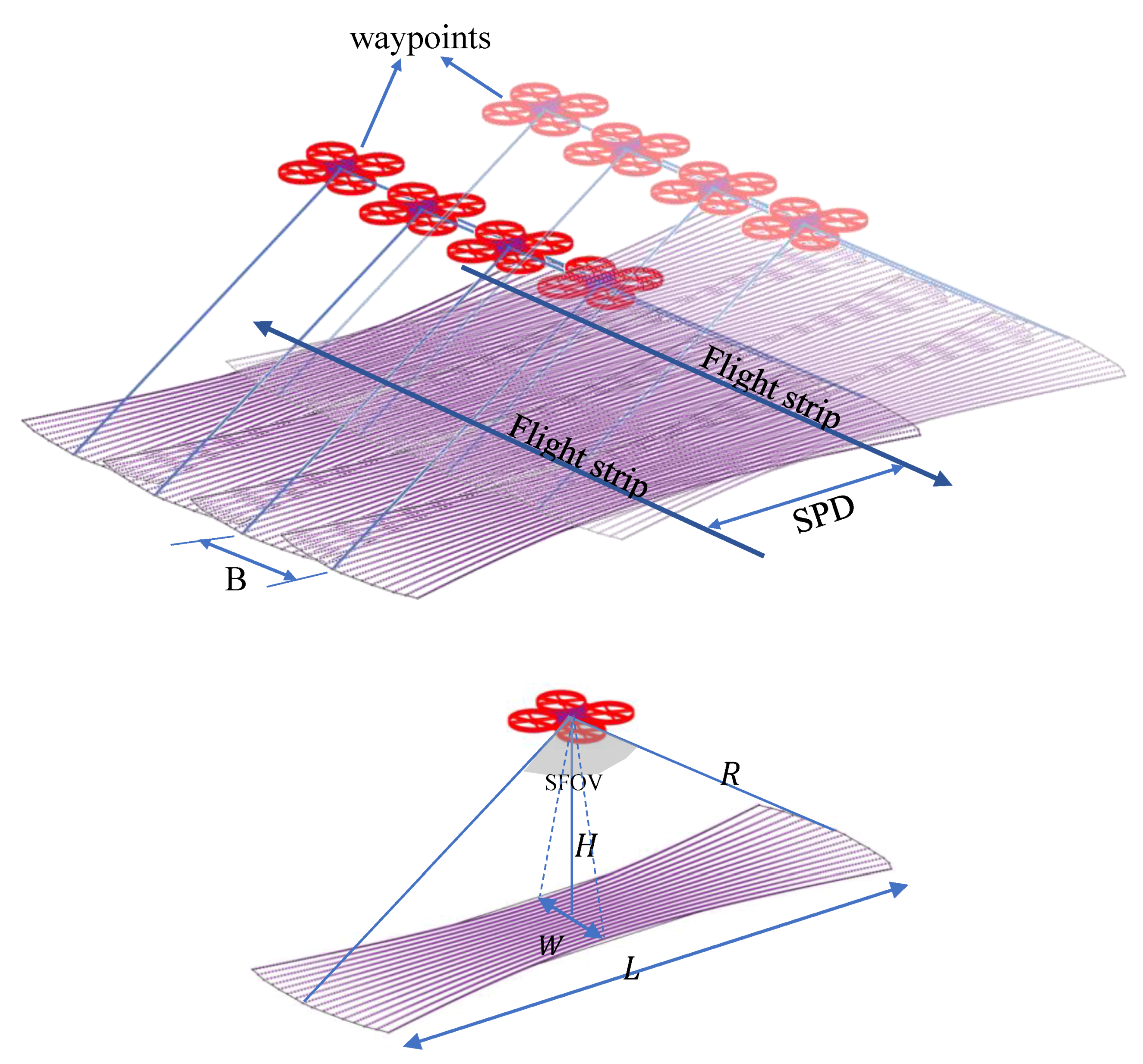
• $L_{area}, W_{area}$: project area dimensions defined as a rectangle with a length $L$ and width $W$.
• $H:$ flying height above the ground level.
• $R:$ scanning range of the LiDAR.
• $B:$ distance between two successive waypoints.
• $W$: along track scanning width.
• $L$: across track swath width of the scanning.
• $SFOV$: scanning field of view out of the offered 360° FOV.
• $SPD$: separation distance between the flight strips.
• $NFS$: number of flight strips rounded to positive infinity.
• $NScan:$ number of waypoints per strip.

After applying the described designation of the flight plan, the UAS waypoints could be determined, where all required information was computed and then maintained to the auto pilot unit of the UAS platform.

In case high objects, like towers or buildings, need to be scanned, the LiDAR-based UAS flight planning tool could be applied by approximating the object of interest with a cylinder, as shown in Figure 4a. Then, the cylinder could be unfolded as a plane that represents the mapping area. Accordingly, the same calculations shown in Equations (1–7) are used, assuming the LiDAR is rotated 90 degrees to the nadir direction. The height of the object would define the length of the mapping area, while the cylinder circumference would define the width of the mapping area. To ensure a complete coverage for the rounded object, the sidelap percentage was preferred to be high (≥80%) in order to result in a smaller separation distance between flight strips. The separation distance would be converted into a central angle $\theta$, to compute the proper angular orientation of the LiDAR device, as shown in Equation (8).

$$\theta =\frac{2\pi }{NFS}$$

(8)

Figure 4b illustrates the relation between the separation distance and the associated angles.

The only significant modification with respect to the described area mapping is to switch the Y and Z coordinates.

2.2. Scanning Simulation

To simulate the UAS LiDAR scans, the scanning points are found when intersecting the LiDAR beams with the ground, assuming a planar ground surface without occlusions. Mathematically, the LiDAR scanning points are computed, as illustrated in Equation (9) [40,41]:

$$\left[\begin{array}{c}{X}_i\\ Y_i\\ Z_i\end{array}\right]=\left[\begin{array}{c}{X}_1\\ Y_1\\ Z_1\end{array}\right]+M\left[\begin{array}{c}R cos\left(Az\right) cos\left(V\right)\\ R sin\left(Az\right) cos\left(V\right)\\ R sin\left(V\right)\end{array}\right]$$

(9)

where

• $R$: the measured range distance from the LiDAR to the object points.
• $M$: rotation matrix of the boresight angles.
• $Az$: the measured azimuth angle of the laser beam.
• $V$: the vertical angle of the laser beam measured from the horizon.
• $X_1, Y_1$, and $Z_1$: the coordinates of the LiDAR sensor.
• $X_i,Y_i,$ and $Z_i$: the coordinates of the scanned point.

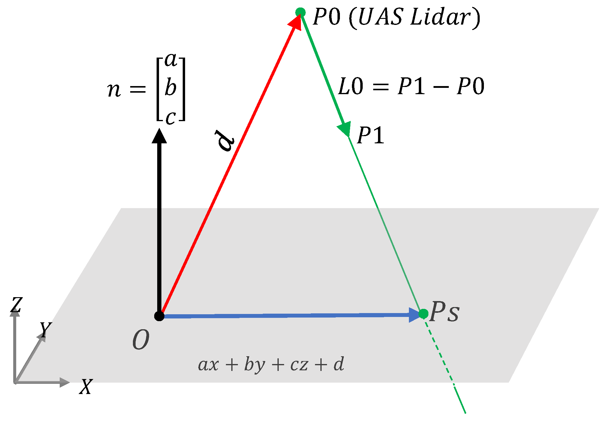
Accordingly, the intersection between every LiDAR beam at time $t$ and the object planes, could be formulated by using the line—plane space intersection calculations, as follows [42]:

-

Compute the scan vector $L$ from the LiDAR $P0 \left[X_1, Y_1,Z_1\right]$ to the object direction point $P1\left[X_i,Y_i,Z_i\right]$. This vector might intersect the simulated object before or after $P1$ at $Ps$ (Figure 5).

-

Define the object plane normal $n$ by the $a, b, c$ parameters.

-

Compute the vector $E$ = $n·L0 (·$ Dot product), which should be a non-zero value if the LiDAR beam line and the object plane are not parallel and should intersect at a unique object point $Ps$.

Based on the vector geometry, the intersection point $Ps$. could be calculated, as in Equation (10):

$$Ps=P0-\frac{\left(ax+by+cz+d\right)}{E} L0$$

(10)

where $ax+by+cz+d$ represents the object plane Equation (Figure 5).

Therefore, if we assume a flat horizontal plane on the ground, the three considered LiDAR sensors produce scanning patters, as shown in Figure 6.

3. Results and Discussion

The flight planning calculation previously presented is hereafter applied to different scenarios, considering different flying speed and altitudes. Results are plotted in graphs for easier understanding and interpretation. Furthermore, to assess the performance of a LiDAR-based UAS scanning in the domain of smart city applications, simulations are executed over a 3D urban area (Section 3.3) and a communication tower (Section 3.4).

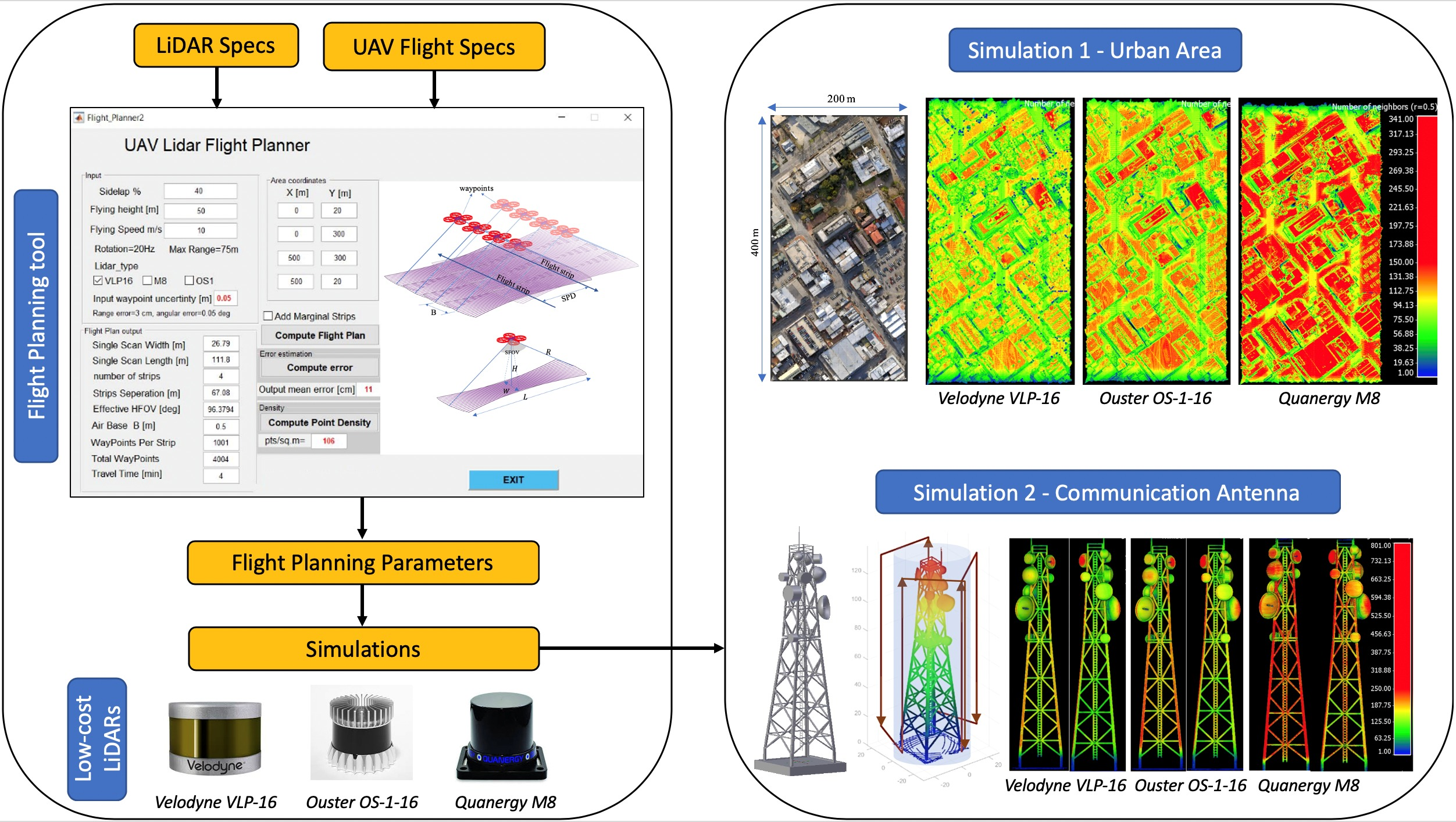
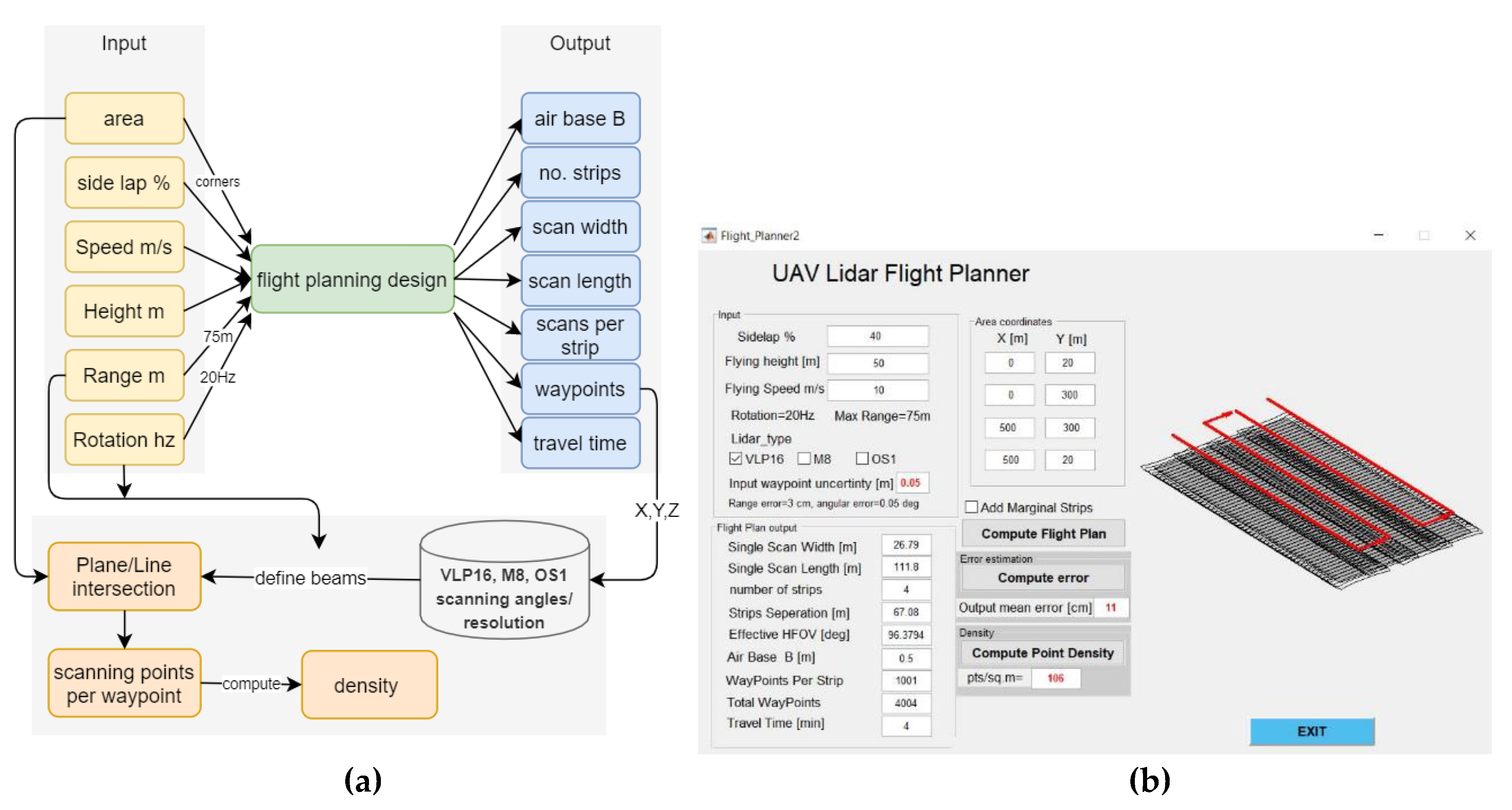
3.1. Flight Planning Tool

The realized MATLAB tool (Figure 7) requires some input parameters such as sidelap percentage, flying height, and UAS flying speed. For the reported tests, the LiDAR rotation is fixed to 20 Hz and the maximum scanning range is fixed to 75 m, within the manufacturer’s specifications.

The developed tool is able to calculate the flight plan parameters including the waypoint coordinates and could be further used for estimating the point density by intersecting the LiDAR beams to the mapping area in analysis. Furthermore, an error propagation could be applied to estimate the average accuracy of the scanned points.

It should be noted that flying at high altitudes would reduce the production rate of the scanning points. However, maximum flying height is restricted by the maximum scanning range of the specific LiDAR sensor in use. Accordingly, the recommended maximum flying height is in the range of 50–80 m for most of the current state-of-the-art low-cost multi-beam LiDARs, in order to ensure significant pulse returns and to comply with the maximum scanning range. On the other hand, whenever the sidelap increases, the number of the designed flight strip increases, the separation distance between strip decreases, and this is expected to result in a higher density of points (Figure 8). However, this larger number of flight strips cost more UAS flying time, which should be carefully considered, especially at low flying speeds, when mapping larger regions.

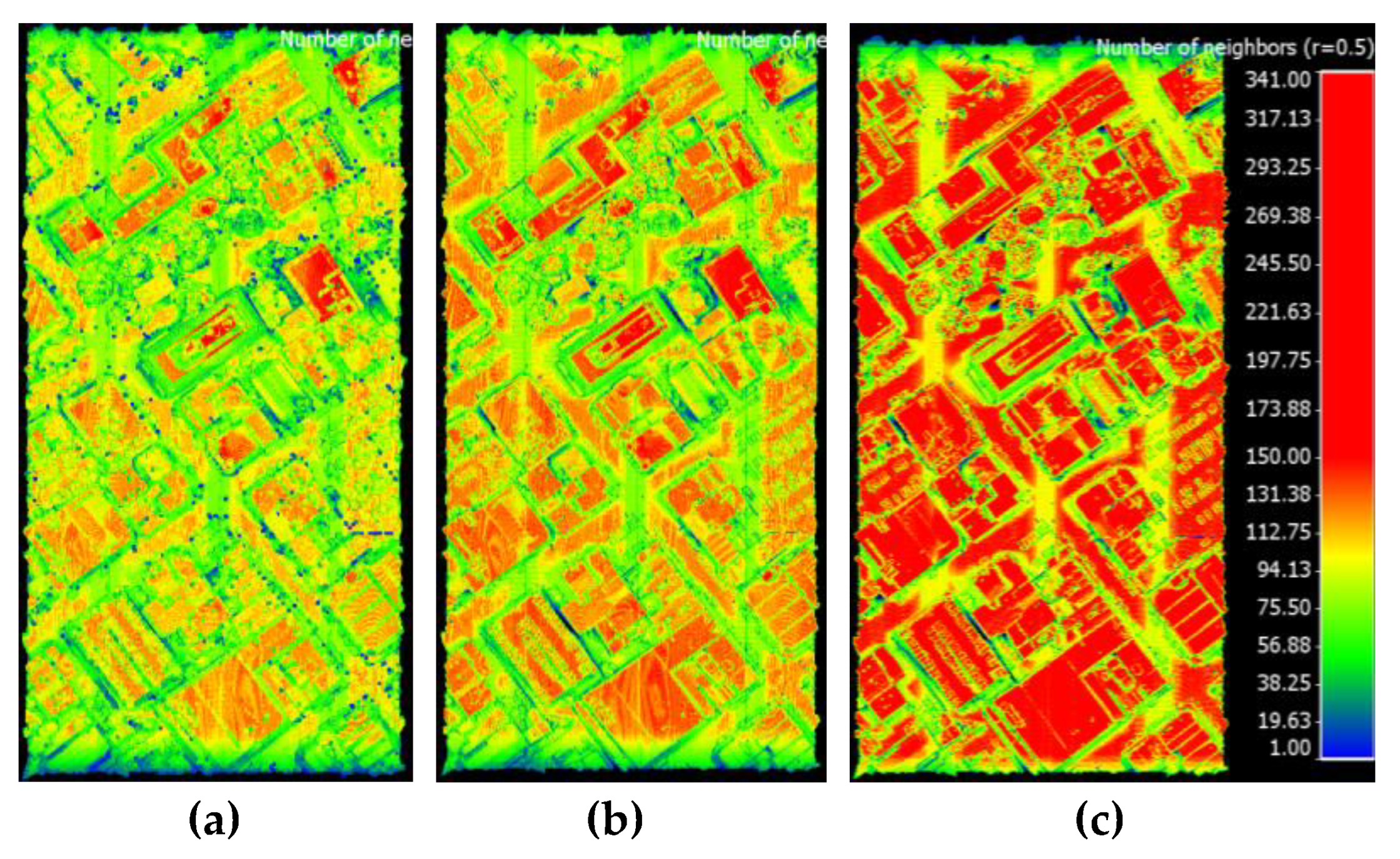
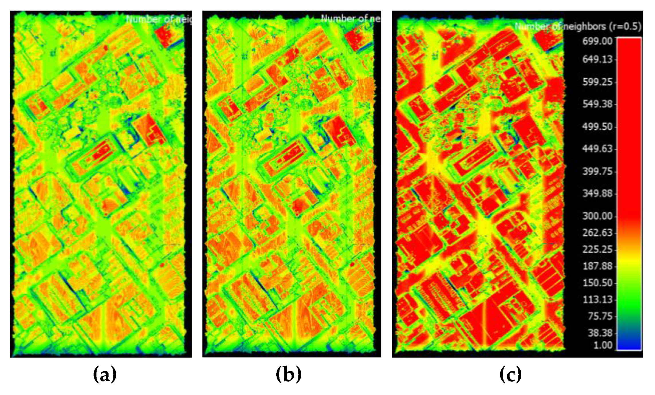
3.2. Estimated Average Point Density

The developed flight planning tool could also be used to estimate the average density of the point cloud acquired using one of the selected spinning multi-beam LiDAR devices. On this basis, a UAS mapping system, equipped with the three different LiDARs of Table 1, was tested for estimating the point density at 10%, 30%, and 50% sidelap percentages, at two flying heights of 30 m (blue) and 60 m (orange), as shown in Figure 9, Figure 10 and Figure 11, respectively.

These graphs were aimed to visualize the relation between the flying speed, flying height, LiDAR type, and the expected point density, which are very useful for users and operators.

Since the sidelap had more influence on the point cloud density compared to the effect of the flying height, a summarized graph is shown in Figure 12 to illustrate the estimated point cloud density related to the flying speeds, at certain sidelap percentages.

Figure 10 shows that the highest achievable point density is at the slower flying speed. It is worth mentioning that the UAS battery life should be considered to determine the allowed maximum flying duration per project. Accordingly, the project area size and the type of the UAS platform would influence the recommended flying speed.

Furthermore, it can be seen how the Quanergy M8 LiDAR is able to produce better densities, compared to the VLP-16 and OS-1-16, despite having half the number of beams. This is related to the smaller horizontal angular resolution, as shown in Table 1.

Additionally, it can be noticed that scanning at higher rotation speed of 20 Hz would ensure better density and scanning coverage compared to the slower frequencies. However, it should be noted that the horizontal angular resolution would be smaller, whenever the rotation frequency is decreased. Another observation from the graphs of Figure 10 is the high attainable density (>1000 pts/m²) below 3 m/s flying speeds of all three investigated UAS LiDAR types, especially at higher sidelap percentages. However, flying at this mentioned slow speed is restricted by different factors like the type of the drone (fixed wing or multi-rotor), the payload weight, etc.

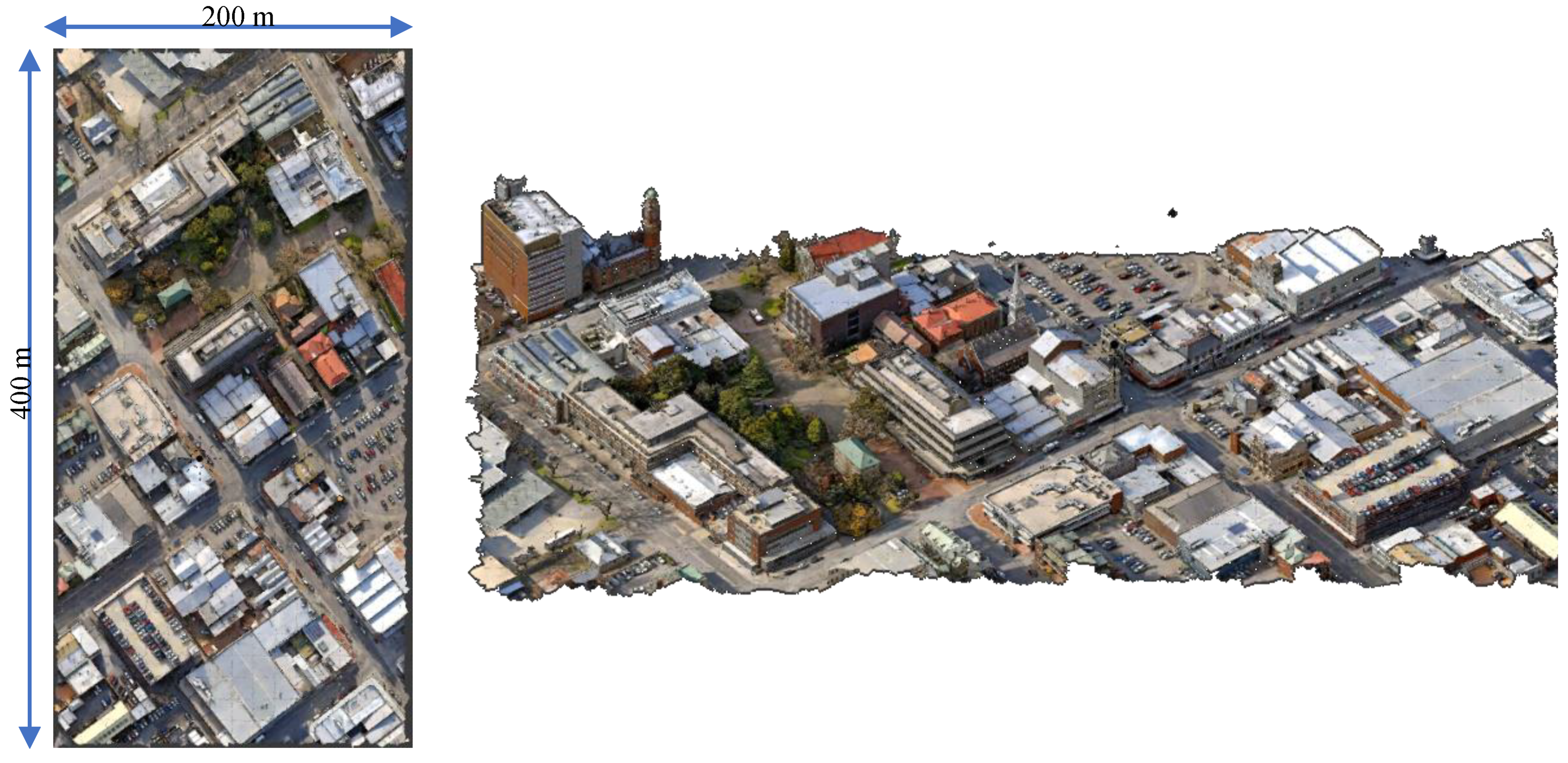
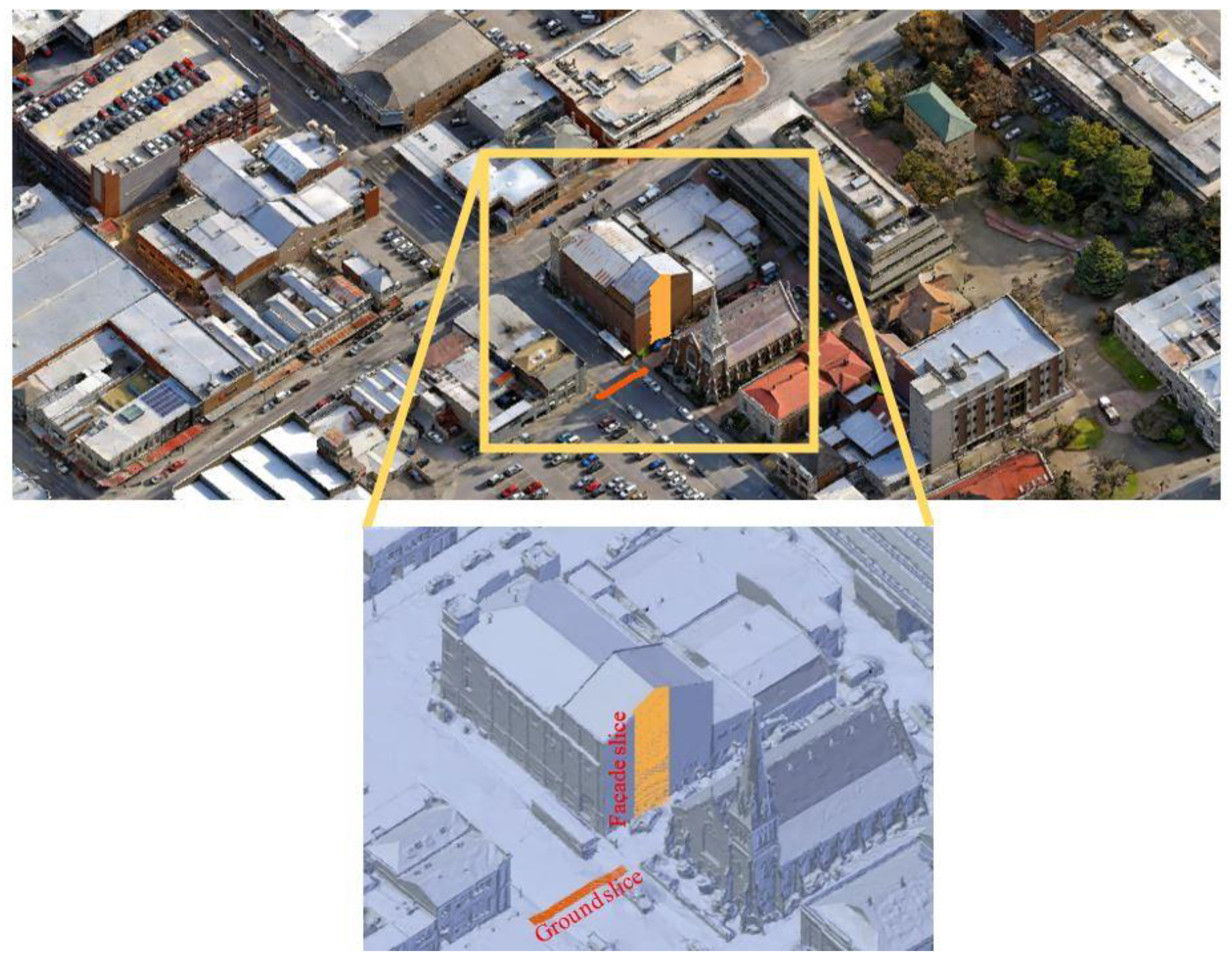
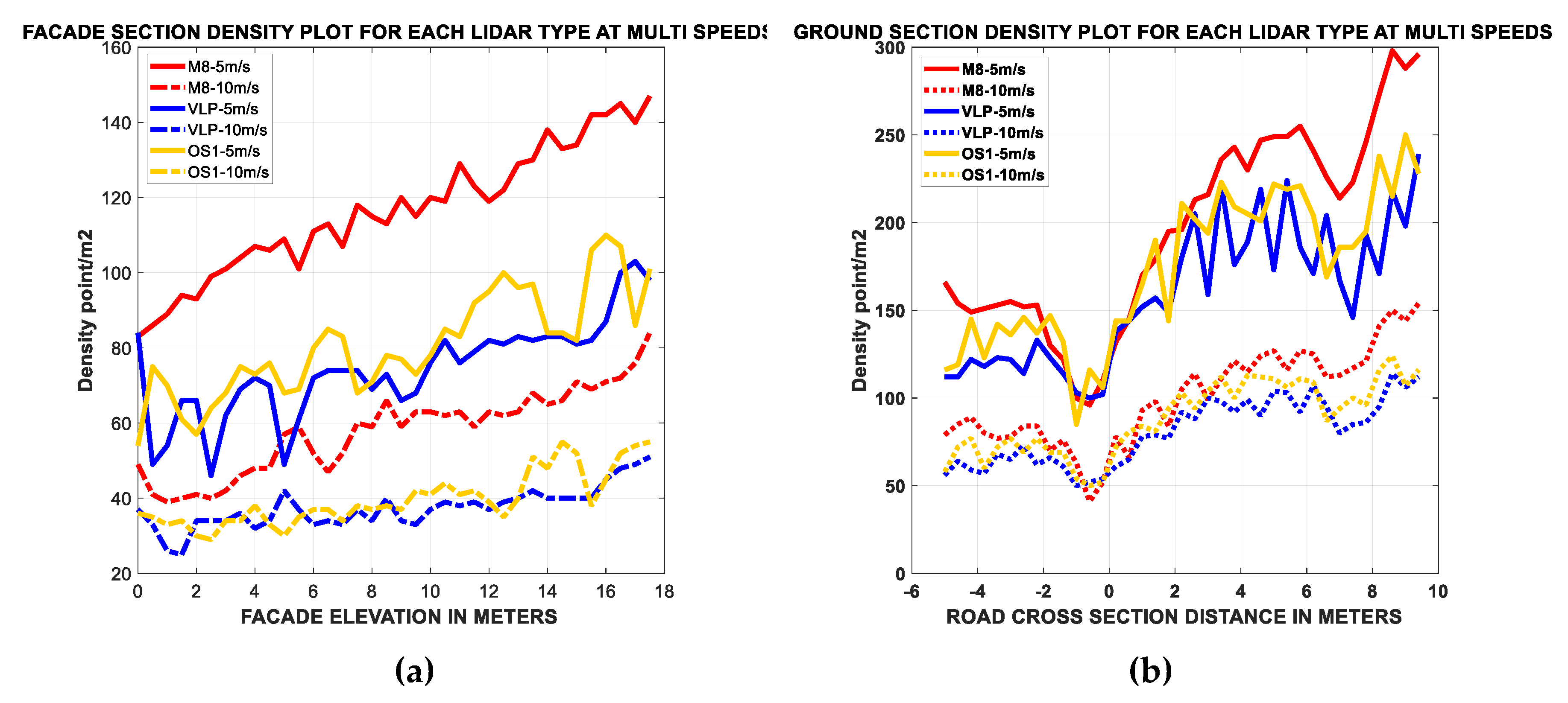
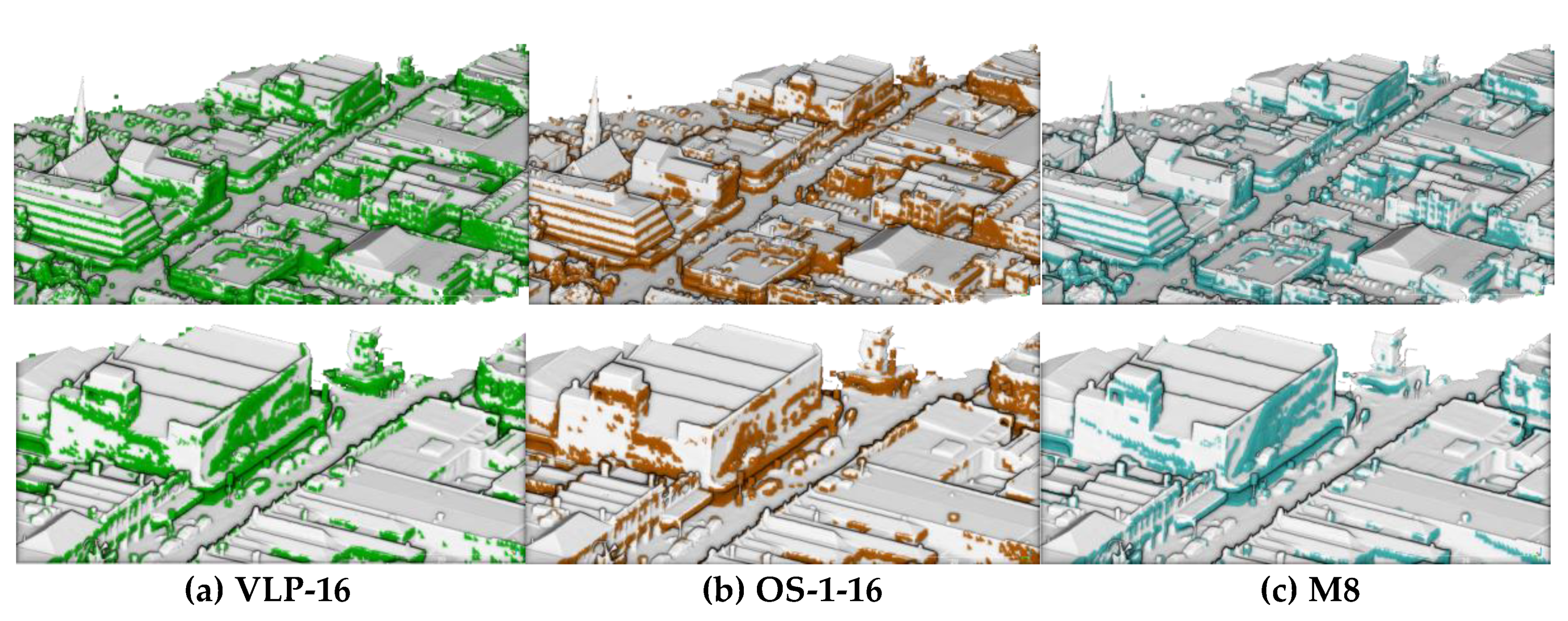
3.3. UAS LiDAR Mapping of an Urban Area

To assess the flight planning design tool and to verify the density plots presented in Section 3.1, a simulation was executed over the 3D urban model of the Lansecton city, Australia [39] (Figure 13).

The three LiDAR sensors were flown at 5 m/s and 10 m/s flying speed. In order to produce a dense point cloud of the urban area, the following design parameters were used—60 m flying height and 30% sidelap (Figure 14). The exported waypoints over five flying strips were modelled using Blender and the scanning simulation was applied using the three mentioned LiDAR sensors.

The resultant point cloud using the UAS platform, equipped each time with one of the selected low-cost LiDAR types, was analyzed (in terms of density) using Cloud Compare [43]. Figure 15 and Figure 16 report the simulations applied at 10 m/s and 5m/s flying speeds, respectively. In Figure 15, the point cloud density is illustrated by selecting a threshold density of 150 pts/m², indicated by a red color. While in Figure 16, the point cloud density is illustrated by selecting a threshold density of 300 pts/m², indicated by the red color.

Although OS-1-16 has the same number of beams as compared to the VLP-16, its point cloud density is higher because of the slightly smaller horizontal resolution and the slightly wider VFOV.

To further elaborate on the density analysis, the derived point clouds were segmented, in order to separate the vertical walls, facades and trees, and the ground and horizontal roofs (Figure 17).

Table 2. Point cloud average density (pts/m²) for the three LiDAR types at two different flying speeds.

	Speed @ 10 m/s		Speed @ 5 m/s
	Facades and Trees	Ground and Horizontal Surfaces	Facades and Trees	Ground and Horizontal Surfaces
M8	81	131	162	260
OS1-1-16	64	105	127	207
VLP-16	58	98	116	192

reports the analyzed density for each class and for each LiDAR sensor, at the two flying speeds.

It could be clearly observed that the density achieved on the facades was less than the density on the ground, due to the nadir orientation of the LiDAR devices. Generally, a linear relation could be noticed between the flying speed and the output density, since halving the flying speed result in approximately doubling the density on the ground and the facade features.

Moreover, two slices were randomly chosen on the ground and on a building façade (Figure 18), with the façade slice located on the cross-track scanning direction.

The point density profile was plotted for every UAS LiDAR mapping system, at each slice, for the two flying speeds at 5 m/s and 10 m/s (Figure 19). What could be noticed from these density graphs was the following:

-

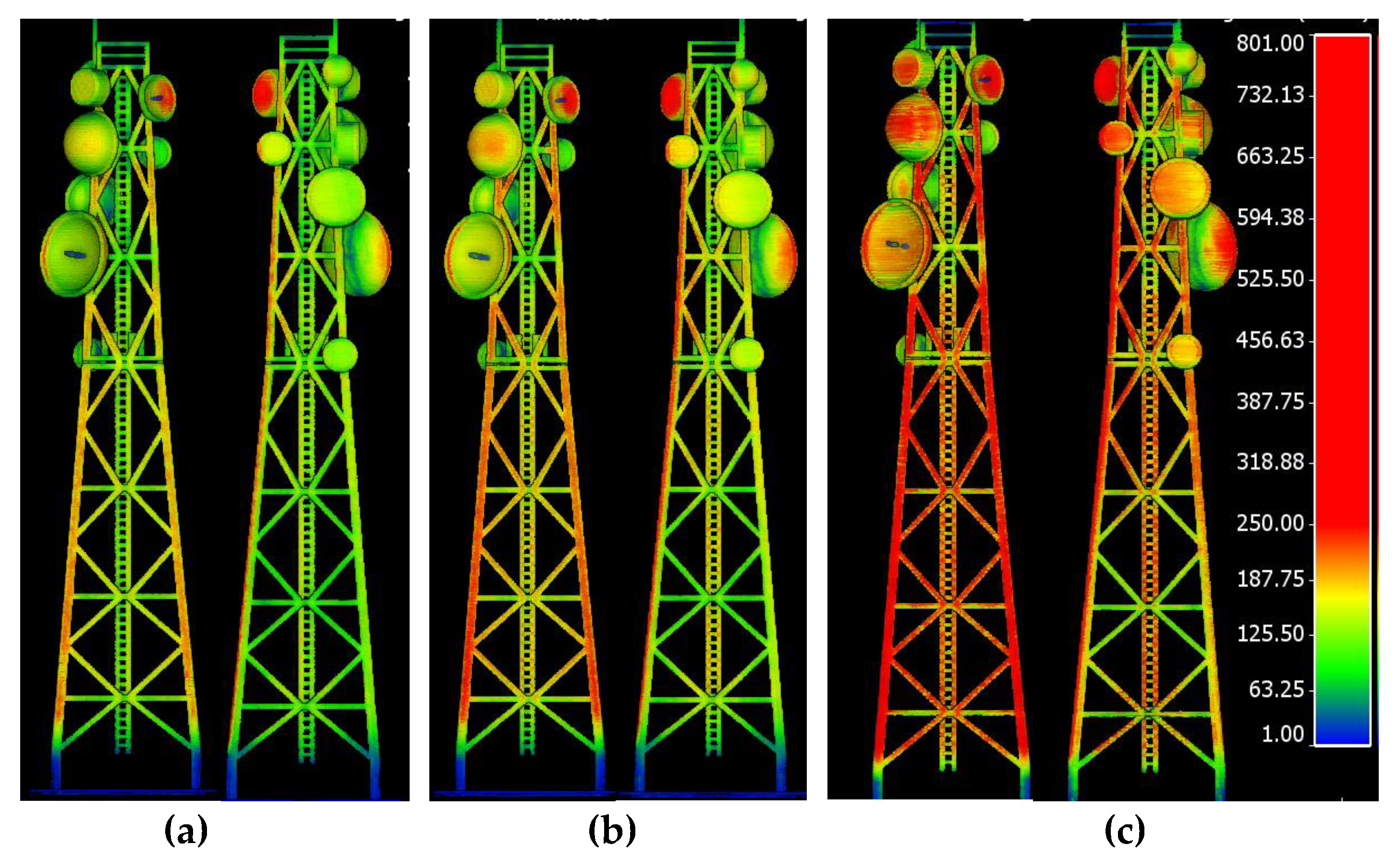
In contrary to the image-based UAS missions, even with the nadir orientation of the LiDAR, a significant coverage and point density on building facades could be attained.

-

M8 had a higher performance than VLP-16 LiDAR and OS-1-16, especially on facade features.

-

Density achieved on facades was approximately half the density achieved on the ground and roof features.

-

Ouster OS-1-16 slightly outperformed the VLP-16 LiDAR on the ground and facades.

-

The density achieved on facades was better at the high altitude parts than the lower altitude parts.

The lack of coverage, as an indication of completeness, could be tested at the three scanned point clouds, since we had the reference 3D model. The completeness could be measured by the following steps:

-

Sample the reference model as a point cloud with a uniform spacing of 10 cm.

-

For every point in the reference point cloud, find any scanning point within a 25 cm search radius.

-

Label reference points as “covered” if they have a neighboring scanned point, or “uncovered” if there are distant scanned points (≥25 cm).

-

Use the “uncovered” points as an indicator of completeness.

Accordingly, the lack of coverage (as percentage) is computed for the three investigated LiDAR types and is illustrated in Figure 20. The analysis showed that Ouster OS -1-16 had a slightly less lack of coverage of 10.7%, as compared to 11.2% using the Quanergy M8 and 11.6% using the Velodyne VLP-16.

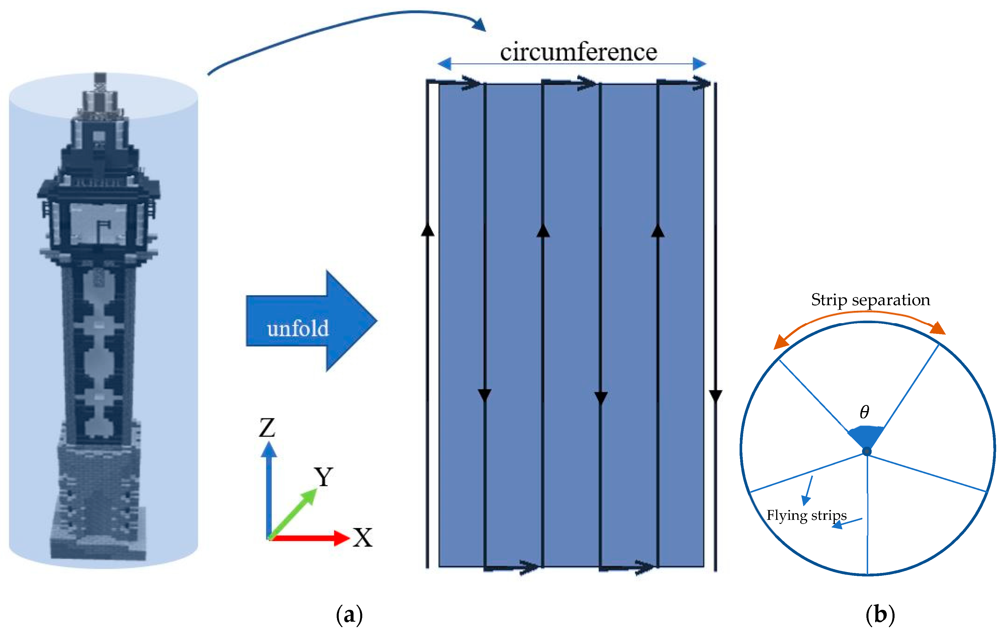
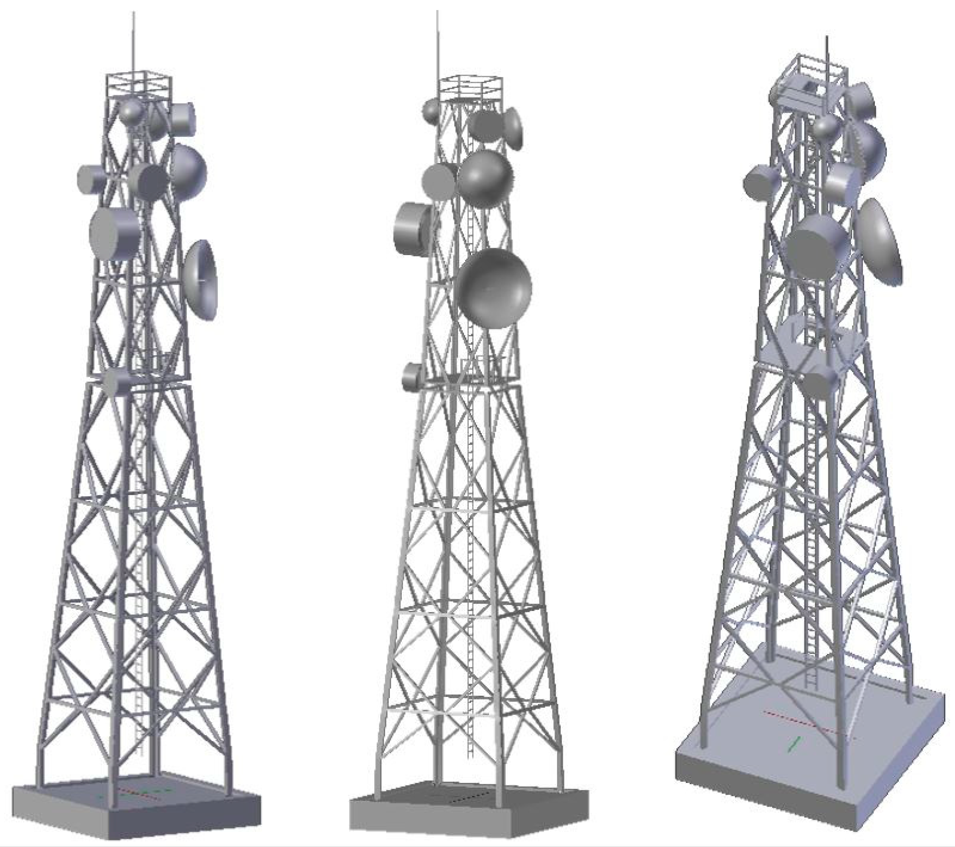
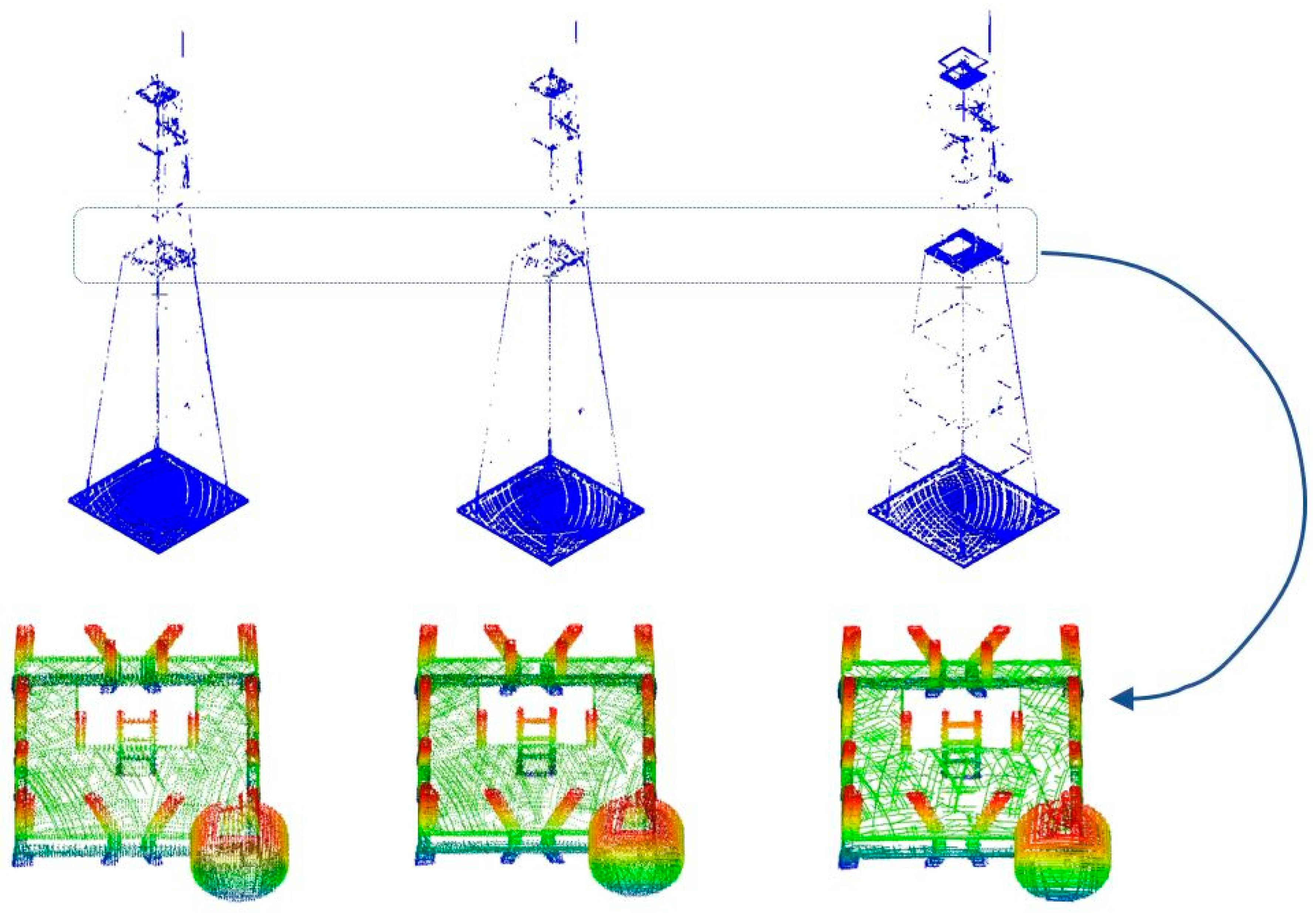
3.4. UAS LiDAR Mapping of a Communication Tower

The proposed flight planning method is tested for the mapping of a communication tall structure. A freely available 3D model of a 120 m communication tower [44] (Figure 21) was used to analyze the results of the three UAS LiDAR mapping systems. Unlike the previous example, featuring large urban areas, here, we consider a vertical structure that required a different mounting form of the LiDAR instrument and a different strip configuration, in order to have a complete survey.

For the flight planning, a high sidelap percentage is preferred, to ensure sufficient overlap coverage for the rounded object, while the flying height would serve in this case for the distance between the UAS LiDAR and the object (Figure 22). The flight planning assumed that (i) a covering cylinder unfolded into a plane, which resulted in six flight strips and (ii) the LiDAR sensors tilted at 90°, and not in a nadir orientation.

The three LiDAR sensors were used in the simulations to assess the achieved point cloud coverage and density. Figure 23 shows the obtained point clouds for each scanning sensor. The point cloud densities were analyzed using Cloud Compare and a threshold of 250 pts/m² was selected (red color) to show the density differences between the three point clouds.

The density achieved using the M8 LiDAR was higher than the densities achieved by OS-1-16 and VLP-16, because of the smaller angular resolution similar to what was observed in the previous experiment in Section 3.2.

The coverage was also evaluated by comparing the resulted point clouds to the reference 3D model. This was done by checking the existence of the neighboring scanned points to every reference point within a threshold distance (i.e., 25 cm). The reference points that were distant to the scanned points were saved for the lack of coverage evaluation. The lack of coverage percentage was calculated by dividing the uncovered points to the total number of the reference points. Figure 24c illustrates that the sensor M8 achieved better coverage on the squared tower base, while lacking some coverage on the horizontal roofs. This could be explained by knowing that the M8 had only 8 beams, compared to 16 beams for the other two investigated types. On the hand, OS-1-16 achieved a better coverage than the VLP-16, as illustrated in Figure 24b, which could be related to the slightly wider FOV of the OS1 LiDAR.

The densities and lack of coverage percentages are listed in

Table 3. Point density and lack of coverage percent.

LiDAR Type	Density pts/m2	Lack of Coverage
VLP-16	162 ± 62	11.1 %
OS-1-16	184 ± 70	8.2 %
M8	235 ± 93	7.6 %

.

4. Conclusions

In this paper, a LiDAR-based UAS flight planning topic was introduced, with a clear mathematical formulation. A prototype software was built using MATLAB and it was shared with the community. Simulations and experiments were performed using three low-cost multi-beam LiDAR sensors—Velodyne VLP-16, Quanergy M8, and Ouster OS-1-16. The paper showed the ability to scan an urban region using a LiDAR sensor in a nadir orientation, or to scan tall structures, like towers and buildings, considering a 90° tilted LiDAR sensor.

Regarding the first research question of the paper, in order to compute the UAS waypoints we need only sidelap, flying height, speed, area of interest, and the LiDAR type. Answers were also given regarding the estimation of the point density in an urban region at different flying heights, sidelaps, and flying speeds, using the selected three low-cost multi-beam LiDAR sensors. Graphical plots were presented to illustrate the relation between point densities and sidelap percentages, at different flying heights and speeds.

In general, the point density could reach 1000 pts/m², when flying at a slow speed of less than 3 m/s for the three LiDAR types, especially when using the Quanergy M8 sensor, which features a smaller horizontal angular resolution. In the experiments with the urban environment and the communication tower, the points density achieved by Quanergy M8 was higher, compared to the point density achieved using Velodyne VLP-16 and Ouster OS-1-16. However, M8 was less efficient in covering horizontal planes.

To the best of our knowledge, the low-cost multi-beam LiDAR Ouster OS-1-16 has not yet been used in a UAS mapping system and, interestingly, it proved to be efficient in terms of density and coverage. Density was comparable or better than the density achieved by the Velodyne VLP-16. If we consider the weight of 450 grams, then it would certainly be a potential candidate for many UAS mapping applications.

So far, the developed tool (https://github.com/Photogrammtery-Topics/UAV-Lidar-flight-planner) is restricted to provide UAS flight planning for the three mentioned types of LiDAR sensors. However, it could be extended to handle any customized LiDAR device, either multi-beam or solid state. Other orientation angles—rather than nadir and 90° orientation—could be added, which might be of interest in urban regions and architectural contexts.

It is worth mentioning that the simulations neglected the effect of wind and other meteorological factors and ideal conditions were assumed. Future work would consider the effect of the mentioned factors and their impact on the performance of UAS LiDAR missions.

Finally, available DTM data could be also included, to consider the non-planarity of the terrain hypothesized so far (Section 2.2).

References

1. Hassanalian, M.; Abdelkefi, A. Classifications, applications, and design challenges of drones: A review. Prog. Aerosp. Sci. 2017, 91, 99–131. [Google Scholar] [CrossRef]
2. Colomina, I.; Molina, P. Unmanned aerial systems for photogrammetry and remote sensing: A review. ISPRS J. Photogramm. Remote Sens. 2014, 92, 79–97. [Google Scholar] [CrossRef] [Green Version]
3. Nex, F.; Remondino, F. UAV for 3D mapping applications: A review. Appl. Geomat. 2014, 6, 1–15. [Google Scholar] [CrossRef]
4. Granshaw, S.I. RPV, UAV, UAS, RPAS … or just drone? Photogramm. Rec. 2018, 33, 160–170. [Google Scholar] [CrossRef]
5. SkyIMD’s Online Flight Planner. Available online: http://www.skyimd.com/online-flight-planner-for-aerial-imaging-mapping-survey/ (accessed on 7 June 2020).
6. Pix4Dcapture. Available online: https://www.pix4d.com/product/pix4dcapture (accessed on 7 June 2020).
7. Oborne, M. Mission Planner. Available online: https://ardupilot.org/planner/index.html (accessed on 7 June 2020).
8. UgCS Software. Available online: https://heighttech.nl/flight-planning-software/ (accessed on 7 June 2020).
9. Flight Planning Software for DJI Drones. Available online: https://www.djiflightplanner.com/ (accessed on 7 June 2020).
10. Drone Mapping. Available online: https://solvi.nu/ (accessed on 7 June 2020).
11. eMotion. Available online: https://www.sensefly.com/software/emotion/ (accessed on 7 June 2020).
12. mdCOCKPIT DESKTOP SOFTWARE. Available online: https://www.microdrones.com/en/integrated-systems/software/mdcockpit/ (accessed on 7 June 2020).
13. UAV Toolbox. Available online: http://uavtoolbox.com/ (accessed on 7 June 2020).
14. UgCS Photogrammetry. Available online: https://www.ugcs.com/ (accessed on 7 June 2020).
15. Almadhoun, R.; Abduldayem, A.; Taha, T.; Seneviratne, L.; Zweiri, Y. Guided Next Best View for 3D Reconstruction of Large Complex Structures. Remote Sens. 2019, 11, 2440. [Google Scholar] [CrossRef] [Green Version]
16. Papadopoulos-Orfanos, D.; Schmitt, F. Automatic 3-D digitization using a laser rangefinder with a small field of view. In Proceedings of the International Conference on Recent Advances in 3-D Digital Imaging and Modeling (Cat. No.97TB100134), Ottawa, ON, Canada, 12–15 May 1997; pp. 60–67. [Google Scholar]
17. Scott, W.R.; Roth, G.; Rivest, J.-F. View planning for automated three-dimensional object reconstruction and inspection. ACM Comput. Surv. 2003, 35, 64–96. [Google Scholar] [CrossRef]
18. Skydio Inc. Available online: https://www.skydio.com/ (accessed on 7 June 2020).
19. Mendoza, M.; Vasquez-Gomez, J.; Taud, H. NBV-Net: A 3D Convolutional Neural Network for Predicting the Next-Best-View. 2018. Available online: https://github.com/irvingvasquez/nbv-net (accessed on 7 June 2020).
20. Vasquez-Gomez, J.I.; Sucar, L.E.; Murrieta-Cid, R.; Lopez-Damian, E. Volumetric Next-best-view Planning for 3D Object Reconstruction with Positioning Error. Int. J. Adv. Rob. Syst. 2014, 11, 159. [Google Scholar] [CrossRef]
21. Haner, S.; Heyden, A. Optimal View Path Planning for Visual SLAM; Springer: Berlin/Heidelberg, Germany, 2011; pp. 370–380. [Google Scholar]
22. Anthony, D.; Elbaum, S.; Lorenz, A.; Detweiler, C. On crop height estimation with UAVs. In Proceedings of the 2014 IEEE/RSJ International Conference on Intelligent Robots and Systems, Chicago, IL, USA, 14–18 September 2014; pp. 4805–4812. [Google Scholar]
23. Teng, G.E.; Zhou, M.; Li, C.R.; Wu, H.H.; Li, W.; Meng, F.R.; Zhou, C.C.; Ma, L. MINI-UAV LIDAR FOR POWER LINE INSPECTION. Int. Arch. Photogramm. Remote Sens. Spatial Inf. Sci. 2017, XLII-2/W7, 297–300. [Google Scholar] [CrossRef] [Green Version]
24. Brede, B.; Lau, A.; Bartholomeus, H.M.; Kooistra, L. Comparing RIEGL RiCOPTER UAV LiDAR Derived Canopy Height and DBH with Terrestrial LiDAR. Sensors 2017, 17, 2371. [Google Scholar] [CrossRef] [PubMed]
25. Mandlburger, G.; Pfennigbauer, M.; Schwarz, R.; Flöry, S.; Nussbaumer, L. Concept and Performance Evaluation of a Novel UAV-Borne Topo-Bathymetric LiDAR Sensor. Remote Sens. 2020, 12, 986. [Google Scholar] [CrossRef] [Green Version]
26. Santiago, R.; Maria, B.-G. An Overview of Lidar Imaging Systems for Autonomous Vehicles. Appl. Sci. 2019, 9, 4093. [Google Scholar]
27. A Complete Guide to LiDAR: Light Detection and Ranging. Available online: https://gisgeography.com/lidar-light-detection-and-ranging/ (accessed on 7 June 2020).
28. Snoopy UAV LiDAR System. Available online: https://www.lidarusa.com/products.html (accessed on 7 June 2020).
29. UAV LiDAR System. Available online: https://www.routescene.com/the-3d-mapping-solution/uav-lidar-system/ (accessed on 7 June 2020).
30. YellowScan Surveyor. Available online: https://www.yellowscan-lidar.com/products/surveyor/ (accessed on 7 June 2020).
31. Geo-MMS LiDAR. Available online: https://geodetics.com/product/geo-mms/ (accessed on 7 June 2020).
32. SCOUT-16. Available online: https://www.phoenixlidar.com/scout-16/ (accessed on 7 June 2020).
33. Geo-MMS: From Flight Mission to Drone Flight Planning. Available online: https://geodetics.com/drone-flight-planning/ (accessed on 7 June 2020).
34. PHOENIX FLIGHT PLANNER. Available online: https://www.phoenixlidar.com/flightplan/ (accessed on 7 June 2020).
35. Quanergy. Available online: https://quanergy.com/ (accessed on 7 June 2020).
36. Ouster. Available online: https://ouster.com/ (accessed on 7 June 2020).
37. Velodyne Lidar. Available online: https://velodynelidar.com/ (accessed on 7 June 2020).
38. Blender. Available online: http://www.blender.org (accessed on 7 June 2020).
39. Launceston City 3D Model. Available online: http://s3-ap-southeast-2.amazonaws.com/launceston/atlas/index.html (accessed on 7 June 2020).
40. Alsadik, B. Adjustment Models in 3D Geomatics and Computational Geophysics: With MATLAB Examples; Elsevier Science: Amsterdam, The Netherlands, 2019. [Google Scholar]
41. Gordon, S.J.; Lichti, D.D. Terrestrial Laser Scanners with A Narrow Field of View: The Effect on 3D Resection Solutions. Surv. Rev. 2004, 37, 448–468. [Google Scholar] [CrossRef]
42. Intersection of Lines and Planes. Available online: http://geomalgorithms.com/a05-_intersect-1.html] (accessed on 15 January 2020).
43. CloudCompare. CloudCompare: 3D Point Cloud and Mesh Processing Software. Available online: https://www.danielgm.net/cc/ (accessed on 7 June 2020).
44. FormAffinity. Communication Tower. Available online: https://www.turbosquid.com/3d-models/free-max-mode-communication-tower/735405 (accessed on 7 June 2020).
Figure 1. Image overlap concept for an image-based flight planning.
Ijgi 09 00378 g001
Figure 2. Flight planning tool and the derived parameters for the simulation analyses in the real-world scenarios.
Ijgi 09 00378 g002
Figure 3. Unmanned aircraft systems (UAS) LiDAR flight planning design parameters.
Ijgi 09 00378 g003
Figure 4. (a) Flight planning for a tower by unfolding a covering virtual cylinder into a plane. (b) A top view showing the conversion of the strip separation distances into angular values.
Ijgi 09 00378 g004
Figure 5. The line–plane intersection in space.
Ijgi 09 00378 g005
Figure 6. Simulated scanning patterns for the selected LiDAR types—Quanergy M8 (a), Velodyne VLP-16 (b), and Ouster OS-1-16 (c).
Ijgi 09 00378 g006
Figure 7. (a) Flowchart of the flight planning tool. (b) Graphical user interface of the designed flight planning tool.
Ijgi 09 00378 g007
Figure 8. Flight plan sketches for mapping a rectangular area at different sidelap percentages, which result in different numbers of flight strips. (a) 10% sidelap—4 strips. (b) 30% sidelap—5 strips. (c) 50% sidelap—6 strips.
Ijgi 09 00378 g008
Figure 9. The relation between the UAS flying speed and the estimated point cloud density at a 10% sidelap, scanned at 30 m (blue) and 60 m (orange) by (a) VLP-16, (b) OS-1-16, and (c) M8.
Ijgi 09 00378 g009
Figure 10. The relation between the UAS flying speed and the estimated point cloud density at a 30% sidelap scanned at 30 m (blue) and 60 m (orange) by (a) VLP-16, (b) OS-1-16, and (c) M8.
Ijgi 09 00378 g010
Figure 11. The relation between the UAS flying speed and the estimated point cloud density at a 50% sidelap, scanned at 30 m (blue) and 60 m (orange) by (a) VLP-16, (b) OS-1-16, and (c) M8.
Ijgi 09 00378 g011
Figure 12. Relation between the point density and the sidelap percentages (50% green, 30% red, 10% blue) at 30 m flying height for (a) VLP-16 (b) OS-1-16, and (c) M8.
Ijgi 09 00378 g012
Figure 13. Two tiles of the Lansecton 3D city model [39] selected to perform the UAS LiDARs tests.
Ijgi 09 00378 g013
Figure 14. (a) The LiDAR-based UAS flight planning for the city model and (b) one scan sweep over the 3D model of the urban area.
Ijgi 09 00378 g014
Figure 15. Point clouds average density maps at 10 m/s speed (red ≥ 150 pts/m2)—86 pts/m2 with (a) VLP-16, (b) 93 pts/m2 with OS-1-16, and (c) 117 pts/m2 with M8.
Ijgi 09 00378 g015
Figure 16. Point cloud average density map at 5 m/s speed (red ≥ 300 pts/m2): 170 pts/m2 with (a) VLP-16, (b) 183 pts/m2 with OS-1-16, and (c) 231 pts/m2 with M8.
Ijgi 09 00378 g016
Figure 17. (a) Segmented point cloud (Cloud Compare)—ground and facades together, (b) vertical façades and tree segments, and (c) ground and horizontal roof segments.
Ijgi 09 00378 g017
Figure 18. Two selected slices, on the ground (orange) and on a building facade (yellow), to check the achieved LiDAR point density.
Ijgi 09 00378 g018
Figure 19. (a) Density on the selected facade slice and (b) the ground slice for Quanergy M8 (red), OS1-16 (yellow), and Velodyne VLP-16 (blue), at two different flying speeds.
Ijgi 09 00378 g019
Figure 20. The completeness (grey) and lack of coverage (colored) in the point clouds acquired by the three UAS LiDAR mapping systems.
Ijgi 09 00378 g020
Figure 21. 3D model of the communication tower (120 m height).
Ijgi 09 00378 g021
Figure 22. Flight planning design for scanning the communication tower.
Ijgi 09 00378 g022
Figure 23. Color-coded visualization of the derived point clouds (red≥ 250 pts/m2) obtained by scanning the tower with the three LiDAR sensors: (a) VLP-16, (b) OS-1-16, and (c) M8.
Ijgi 09 00378 g023
Figure 24. Lack of point cloud coverage (1st row) and the selected enlarged point cloud segments (2nd row) obtained by scanning the tower with the VLP-16 (a), OS-1-16 (b), and M8 (c) LiDAR sensors.
Ijgi 09 00378 g024