Performance Evaluation and Comparison of Bivariate Statistical-Based Artificial Intelligence Algorithms for Spatial Prediction of Landslides

Abstract

The purpose of this study is to compare nine models, composed of certainty factors (CFs), weights of evidence (WoE), evidential belief function (EBF) and two machine learning models, namely random forest (RF) and support vector machine (SVM). In the first step, fifteen landslide conditioning factors were selected to prepare thematic maps, including slope aspect, slope angle, elevation, stream power index (SPI), sediment transport index (STI), topographic wetness index (TWI), plan curvature, profile curvature, land use, normalized difference vegetation index (NDVI), soil, lithology, rainfall, distance to rivers and distance to roads. In the second step, 152 landslides were randomly divided into two groups at a ratio of 70/30 as the training and validation datasets. In the third step, the weights of the CF, WoE and EBF models for conditioning factor were calculated separately, and the weights were used to generate the landslide susceptibility maps. The weights of each bivariate model were substituted into the RF and SVM models, respectively, and six integrated models and landslide susceptibility maps were obtained. In the fourth step, the receiver operating characteristic (ROC) curve and related parameters were used for verification and comparison, and then the success rate curve and the prediction rate curves were used for re-analysis. The comprehensive results showed that the hybrid model is superior to the bivariate model, and all nine models have excellent performance. The WoE–RF model has the highest predictive ability (AUC_T: 0.9993, AUC_P: 0.8968). The landslide susceptibility maps produced in this study can be used to manage landslide hazard and risk in Linyou County and other similar areas.

1. Introduction

Landslides cause various types of damage and affect people’s lives and property [1]. In order to reduce these losses and hazards, relevant assessments of slope conditions where landslides are likely to occur should be made, and a series of countermeasures should be developed based on the combined assessment results [2]. The definition of landslide susceptibility can be regarded as the tendency of a landslide in a region [3,4]. A landslide susceptibility map is a basic source for representing landslide-prone areas and is a key source for decision-makers, planners, geologists and civil engineers to provide valuable information that provides the necessary information to establish monitoring systems within the study area or to develop measures that may guarantee human life and property [5,6]. The reliability of landslide susceptibility maps depends on the quantity and quality of available data, the scale of work and the choice of modeling methods [7].

Geographic Information Systems (GIS) and remote sensing (RS) are excellent and useful tools for collecting spatial data from the real world and for mapping landslide susceptibility in specific areas [8,9]. In recent decades, thanks to the development of GIS and RS technologies, receiving data used in GIS has become easier and faster, and these tools have contributed greatly to disaster assessment [1,5,10,11]. Therefore, the application of GIS in landslide susceptibility analysis is becoming more and more popular [12,13].

Many researchers have applied heuristic, deterministic, statistical and soft computing models to assess landslide susceptibility. Due to their subjectivity, heuristic methods usually need to add more complex techniques to the overall method to evaluate landslide susceptibility [4,14,15,16]. The deterministic method is only applicable to small areas with simple landslide types and relatively simple and uniform rock and soil mass [17]. Therefore, in order to avoid unnecessary trouble and to reduce the deviation of the above two methods, statistical and soft computing models are usually selected for large-scale and complex landslide susceptibility assessment [6]. In recent years, a variety of statistical methods and soft computing models have been used for landslide susceptibility assessment [18,19,20,21,22], such as support vector machines [23,24,25,26], random forest [27,28,29], artificial neural network [30,31,32,33], decision trees [34,35,36,37], classification and regression tree [38,39], maximum entropy [40,41,42], naïve Bayes [43], neuro-fuzzy [44,45], kernel logistic regression [46,47], alternating decision trees [48,49,50] and boosted regression trees [51].

Recently, several hybrid integration methods have been developed, such as integration of Radial Basis Function neural network and Rotation Forest [52], and adaptive neuro-fuzzy inference system with grey wolf optimizer [53]. The core value of the integrated method is that it has higher accuracy in identification and better prediction ability than the single machine learning model [54,55]. This function can greatly increase the impact of the technology and assist researchers in their analysis of future landslides [12].

Both bivariate models and machine learning models have been widely used in landslide susceptibility research. The advantage of the bivariate model is that it can assess the impact of factor categories on the occurrence of landslides. It is easy to overlook the interrelationship between these factors; however, machine learning models can make up for this shortcoming [56]. Therefore, it is necessary to carry out hybrid landslide modeling on the bivariate model and the machine learning model. The biggest advantage of this hybrid model is that it can comprehensively evaluate the independent variables related to landslides in each type of independent layer [57]. In this study, we aim to propose and verify the overall effect of the bivariate statistical-based random forest and support vector machine for spatial prediction of landslides in Linyou County, China.

2. Materials and Methods

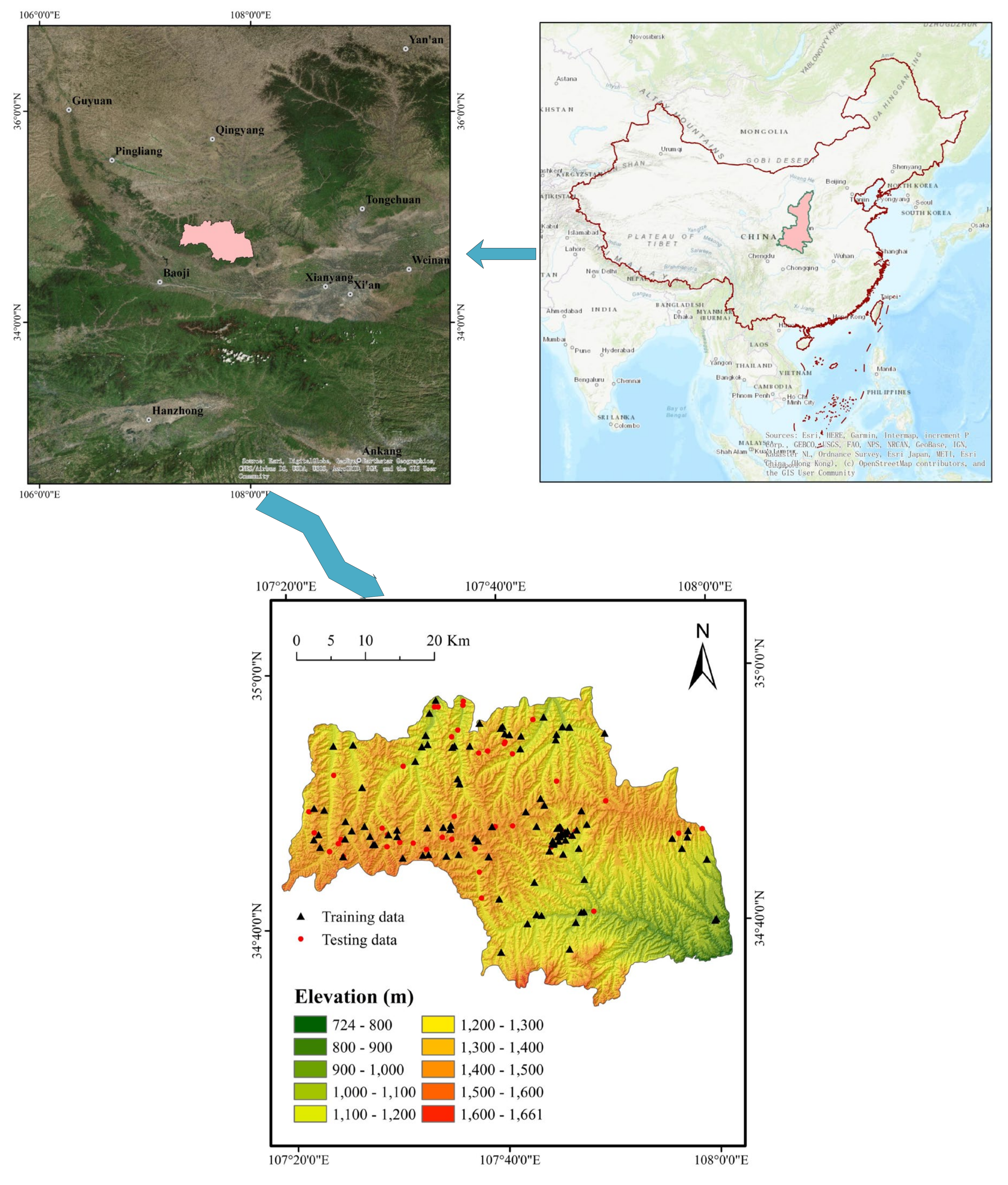
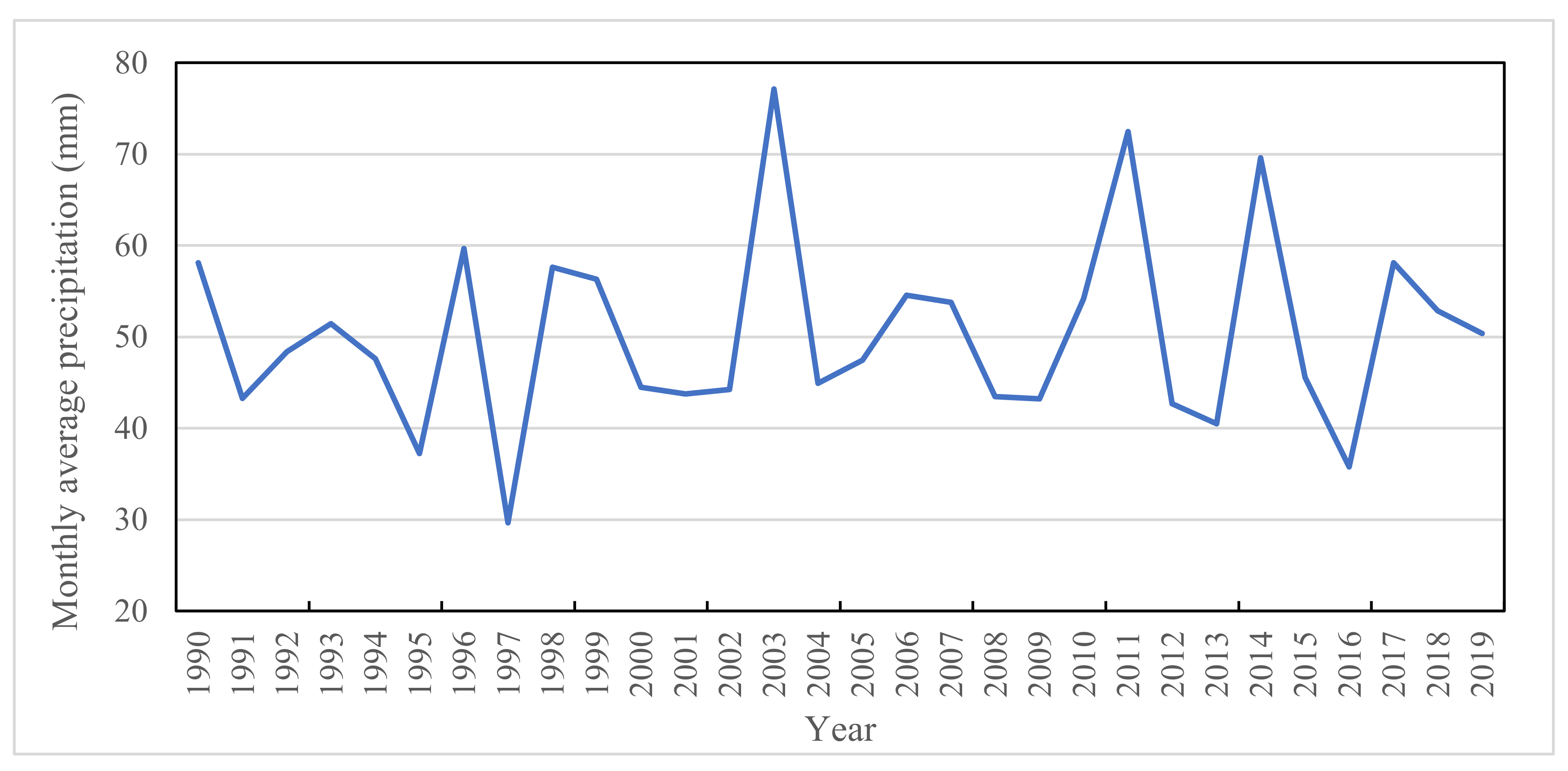
2.1. Study Area

Linyou County of Baoji City is located in the south of the Loess Plateau, with Qishan mountain in the south, Liupan Mountain and its branch Longshan mountain in the west and the Loess Plateau and Beishan Mountain on its southern edge in the north. The overall terrain is high in the northwest and low in the southeast. The average altitude of the whole territory is 1271 m, the highest altitude is 1661 m and the lowest altitude is 724 m (Figure 1). The entire area can be divided into four types of geomorphic units: the hilly area of low and middle mountains, loess hilly area, loess remnant tableland and river valley channel. Linyou County is located in the upper reaches of Qishui River, a tributary of Wei River. Its topography is complex, and the density of rivers and gullies is large, with 0.79 per square kilometer.

The study area belongs to a temperate semi-humid–humid monsoon climate zone. There are four distinct seasons, with short summers and long winters. In the past 30 years (1990–2019), the maximum annual rainfall was 925.4 mm, the minimum annual rainfall was 355.8 mm and the average annual precipitation was 603.3 mm (Figure 2).

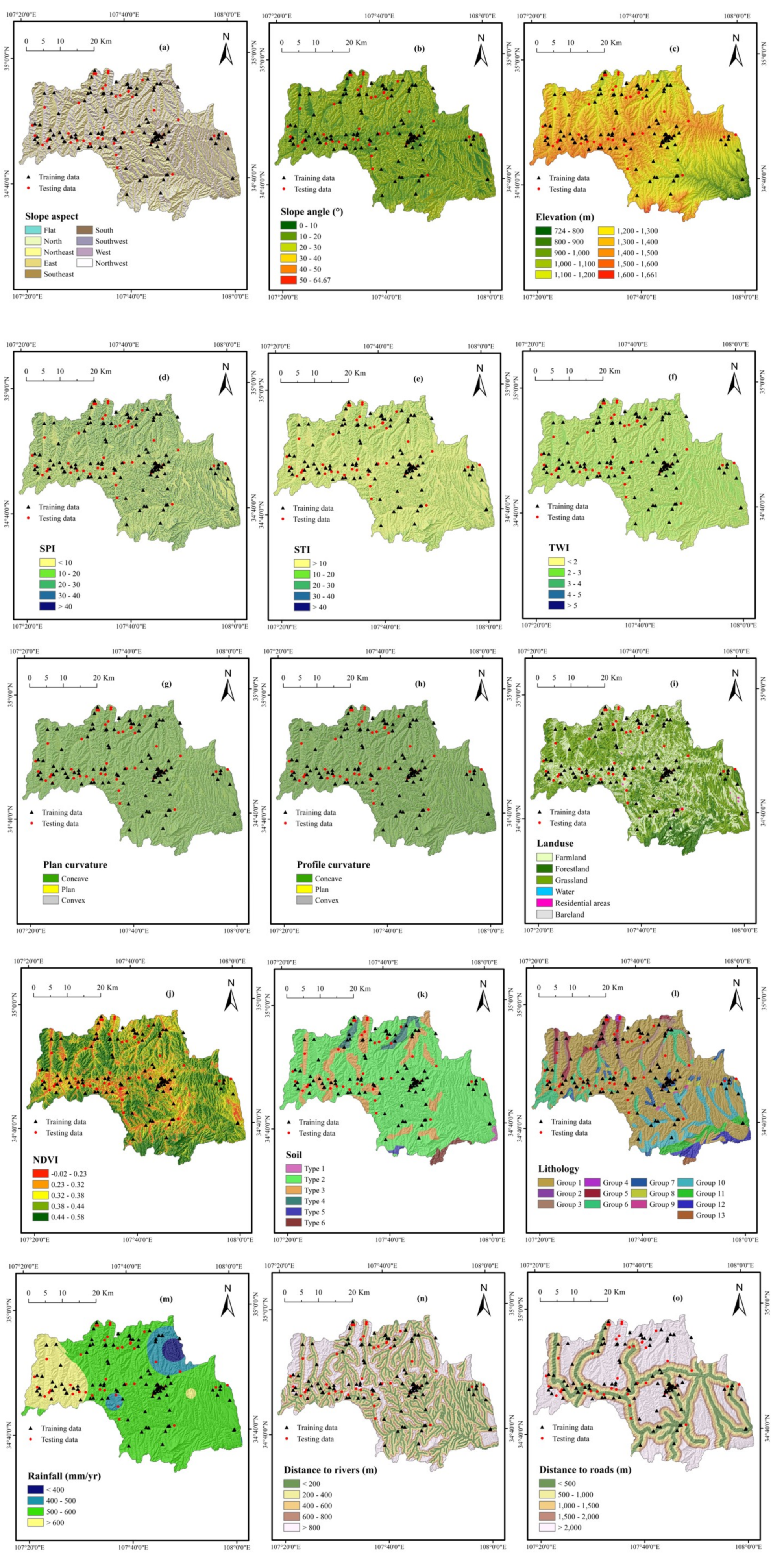
2.2. Data Preparation

The thematic map of landslide inventory constitutes the basis for the prediction of landslide susceptibility [58]. In this study, 152 landslides were identified through early reports, remote sensing image interpretation and field investigations [45]. Each landslide polygon in the landslide dataset is represented by a centroid [59]. In order to identify whether landslides are likely to occur in the area, it is necessary to prepare the same number of non-landslide data. Specifically, 152 non-landslide points were randomly selected from areas where landslides did not occur. The landslide data were randomly divided into two parts according to a ratio of 70/30, respectively, forming two sets of data, namely training data and verification data [60].

Relevant factors were selected to predict the occurrence of landslide hazards according to the characteristics of the study area and previous similar studies [61,62]. In the study area, landslide susceptibility evaluation was carried out using fifteen landslide conditioning factors, namely slope aspect, slope angle, elevation, stream power index (SPI), sediment transport index (STI), topographic wetness index (TWI), plan curvature, profile curvature, land use, normalized difference vegetation index (NDVI), soil, lithology, rainfall, distance to rivers and distance to roads (Figure 3).

The slope aspect affects the discontinuity, the sunshine time and the intensity of solar radiation [63]. The slope aspect map includes nine categories: flat, south, north, southwest, northeast, west, east, northwest and southeast. The slope angle indicates the steepness of the slope, which affects the size and shear strength of the potential slip surface. The slope angle ranges from 0° to 64.67°, and it was divided into 6 categories with 10° intervals. Elevation has a great influence on the degree of rock weathering, and it is an indispensable factor for the prediction of landslide susceptibility [64]. The elevation range is 724–1661 m, which is divided into ten subcategories. SPI indicates the erosion capacity of the water flow [65]. STI describes the potential erosive force of slope flow [66]. SPI and STI were divided into five categories: <10, 10–20, 20–30, 30–40 and >40. TWI can indicate runoff trends and catchment locations. TWI was divided into five categories: <2, 2–3, 3–4, 4–5 and >5. Plan curvature and Profile curvature were divided into three categories: concave, plan and convex. Landuse was divided into six categories: farmland, forestland, grassland, water, residential areas and bareland. NDVI is used to measure vegetation trends that affect the mechanical properties of slopes and hydrological processes related to the instability of the land and slopes in the study area [67,68]. The NDVI values range from −0.02 to 0.58 and were divided into five subcategories. Soil affects the movement of groundwater and surface water, and its physical and mechanical properties vary depending on the type of soil [69,70]. The soil map includes six categories, namely fimic anthrosol, calcaric cambisol, eutric cambisol, gleyic cambisol, calcaric regosol and eutric regosol. Lithology is very important for the occurrence of landslides, and has a great influence on the scale, type, distribution and activity nature of landslides [71]. The lithology is divided into 13 groups. Rainfall can cause a decrease in shear strength and induce landslides [72,73]. Rainfall categories in the study area include: <400, 400–500, 500–600 and >600. Distance to rivers determines the water content of the rocks and soil that make up the main slope [74]. The distance to rivers map includes five buffers: <200, 200–400, 400–600, 600–800 and >800. The construction of a road will affect the stability of the slope angle [75,76]. Therefore, distance to roads affects slope stability. The distance to roads map includes five buffers: <500, 500–1000, 1000–1500, 1500–2000 and >2000. Finally, all thematic maps were resampled and converted to the same resolution (20 m × 20 m).

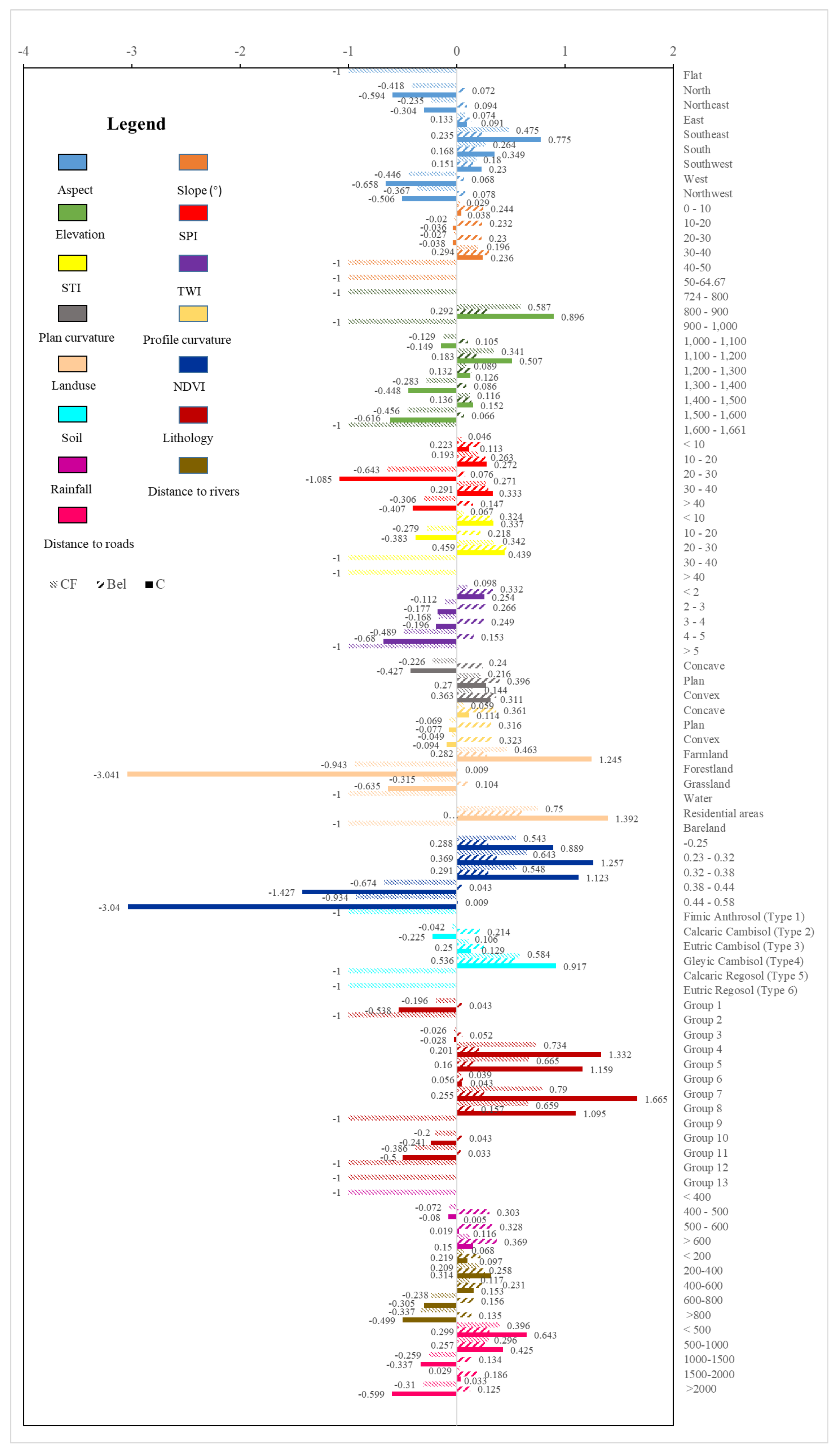
2.3. Certainty Factors (CFs)

The CF model was first proposed in 1990 [77] and modified subsequently [78]. CF can be expressed as follows:

$$CF={\{}_{\frac{PPa-PPs}{PPs(1-PPa)}{{\displaystyle }}_{}^{}\hspace{1em}if\hspace{1em}PPa<PPs}^{\frac{PPa-PPs}{PPa(1-PPs)}{{\displaystyle }}_{}^{}\hspace{1em}if\hspace{1em}PPa\ge PPs}$$

(1)

where PPa is the conditional probability in class a, PPs is the prior probability of the total study area [79].

The change range of CF to [−1, 1] is such that the larger the value is, the more likely the landslide will occur. When the CF value approaches 0, it is difficult to give the certainty of the landslide, because the prior probability is the same as the conditional probability.

2.4. Weights of Evidence (WoE)

WoE is based on the Bayesian probability model and uses logarithmic linear form [80]. The main objective of WoE is to determine the spatial relationship between landslides and conditioning factors [81].

$$W^{+}=ln\frac{P\left\{B\left|A\right.\right\}}{P\left\{B\left|\overline{A}\right.\right\}}$$

(2)

$$W^{-}=ln\frac{P\left\{\overline{B}\left|A\right.\right\}}{P\left\{B\left|\overline{A}\right.\right\}}$$

(3)

$$C=W^{+}+W^{-}$$

(4)

where P represents the probability, B represents each category of each factor and $\overline{B}$ represents each category of non-members of each factor. The pixel point A represents the occurrence of landslide, while $\overline{A}$ represents non-landslide. $W^{+}$ indicates the positive correlation between each category and landslide. $W^{-}$ indicates the negative correlation between category and landslide. C indicates the correlation between landslide and category characteristics [82].

2.5. Evidential Belief Function (EBF)

EBF method is mainly based on the evidence theory algorithm of Dempster–Shafer [83]. EBF is the sum of Bel (degree of belief), Dis (degree of disbelief), Unc (degree of uncertainty) and Pls (degree of plausibilities), and its range is [0, 1] [84]. Bel is used to expressing the correlation between landslide and conditioning factors in the study, and it is expressed using the following formula [85]:

$$Belief\left(\mathit{Bel}\right)=\frac{Be{l}_1+Be{l}_2+L+Be{l}_n}{1-{\displaystyle {\sum }_{i=2}^{n}Be{l}_{i-1}Di{s}_i-Di{s}_{i-1}Be{l}_i}}$$

(5)

where $Be{l}_n$ denotes the elements of each type or range.

2.6. Random Forest (RF)

RF is a powerful integrated learning model proposed by Breiman in 2001 [86]. It has outstanding performance in classification, regression and unsupervised learning [87,88]. In the RF model, the landslide conditioning factor iP (random variable) and a previous random variable are generated independently and distributed on the binary decision tree. The training and verification dataset and random vector i_P are grown on two trees (landslides and non-landslides), and the set of the tree structure classification $h\left(x,\hspace{1em}{i}_p\right),\hspace{1em}p=1,2,\dots n$ of input variable x is obtained. Generally, in RF method, generalization error is shown as follows [89]:

$$generalization error=P_{x,y}\left(mg\left(x,y\right)<0\right)$$

(6)

$$mg\left(x,y\right)=a{v}_{p}I\left(h_p\left(x\right)=y\right)-{\max }_{j\ne y}a{v}_{p}I\left(h_p\left(x\right)=j\right)$$

(7)

where x and y represent the landslide conditioning factors, mg is the margin function and I is the indicator function [86].

2.7. Support Vector Machine (SVM)

SVM is a non-linear classification system based on structural risk minimization and Vapnik-Chervonenkis dimension, which can be used for assortment and recurrence [90]. It separates classes from decision-making areas and maximizes the gap between classes [91]. This method can find an optimal hyperplane for binary classification problems to separate the two classes [92].

In this study, we used the radial basis function with optimum $\phi \left(m,m_i\right)=\exp \left\{-\gamma {‖m-m_i‖}^2\right\}$ [93]. The decision function of SVM can be expressed by the following formula [92]:

$$f\left(m_i\right)=\mathrm{sign}\left[{\displaystyle \sum _{i=1}^{\mathrm{n}}{\eta }_i{n}_i\exp \left\{-\gamma {‖m-m_i‖}^2\right\}+u}\right]$$

(8)

where $\gamma$ is used as the kernel parameter and ${\eta }_i$ is used as the Lagrange multiplier.

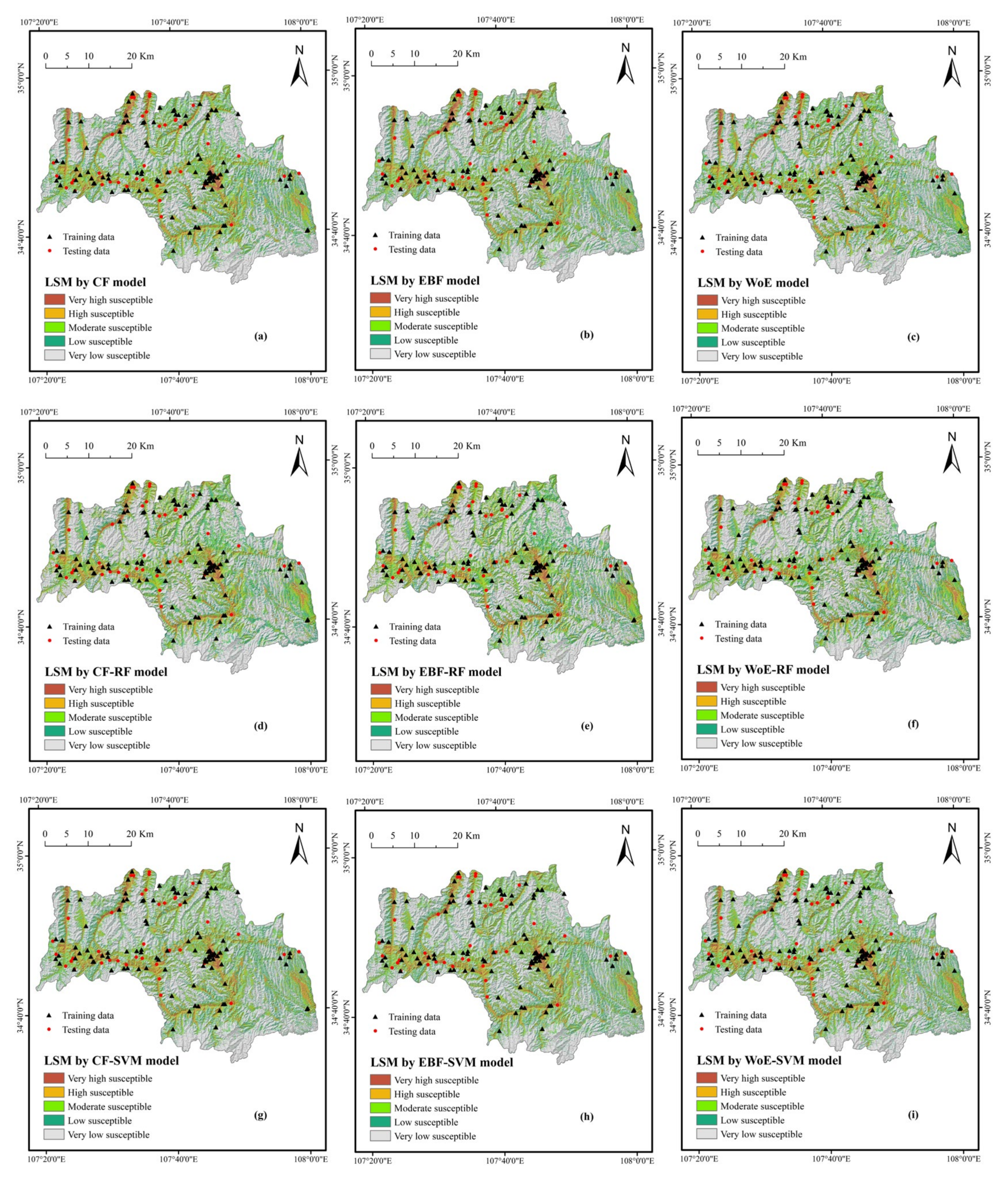
3. Results and Analysis

3.1. Application of the CF Model

The CF model was applied to each class of the landslide conditioning factors, and the CF weights were computed as shown in Figure 4. It is noted that the positive CF weights indicate the higher impact of the class of the conditioning factors on landslide occurrence. Accordingly, in terms of slope aspect, the results show that southeast (CF = 0.475), south (CF = 0.264), southwest (CF = 0.180) and east (CF = 0.074) were the most important classes for landslide incidence. However, the northeast, northwest, north, west, and flat had the least effect due to having negative CF weights. In terms of slope angle, the results showed that the slope angle between 30° and 40° had the highest potential for landslide occurrence (CF = 0.196). Slope angles lower than 10° were ranked in the next position with CF weight equal to 0.029, and other slope angle classes were not more effective and assigned by negative weights so that slope angles more than 40° did not play any role in landslide occurrence (CF = −1). Elevations between 800 and 900 m (CF = 0.587), 1100 and 1200 m (CF = 0.341), 1200 and 1300 m (CF = 0.089) and 1400 and 1500 m (CF = 0.116) were positively correlated with the occurrence of landslides in the study area. Another conditioning factor, SPI, analyzed based on CF weight, showed that SPI between 30 and 40 (CF = 0.271) had the greatest potential for landslide occurrence. It is followed by SPI between 10 and 20 (CF = 0.193) and SPI lower than 10 (CF = 0.046). This indicates that these classes of SPI were more prone to landslide occurrence compared to other classes. Analysis of CF weights for STI illustrated that the values between 30 and 40 and lower than 10 assigned a CF equal to 0.342 and 0.067 and thus concluded that they were more susceptible compared to other classes of STI for landslide occurrence. In the case of TWI, the result of CF weights indicated that lower TWI values (<2) obtained the highest CF value (0.098). According to Figure 1, 66 landslide locations occurred only at this class of TWI. Additionally, results showed that the higher the TWI was, the lower the potential for landslide incidence would be. In terms of plan curvature, results showed that plan (CF = 0.216) and convex (CF = 0.144) slope forms and, in the case of plan curvature, concave slope form (CF = 0.059) were the most important on landslide occurrence in the study area.

3.2. Application of EBF Model

In this study, the EBF model was performed, and the result is reported based on the “Bel” index, which is shown in Figure 4. The higher the Bel weight of each class of the conditioning factor was, the higher the potential of the class would be. The southeast slope aspect was the most important class among other slope aspect classes (Bel = 0.235) to landslide occurrence. It is followed by south (Bel = 0.168), southwest (Bel = 0.151), east (Bel = 0.133), northeast (Bel = 0.094), northwest (Bel = 0.078), north (Bel = 0.072), west (Bel = 0.068) and flat (Bel = 0.000). In the case of slope angle, results showed that slope angles lower than 40° were more susceptible and had more potential for landslide occurrence. Among all classes, slope angles between 30° and 40° had the greatest impact on landslides of the study area (Bel = 0.294). This was followed by 0°–10° (0.244), 10°–20° (0.232) and 20°–30° (0.230). Although only two landslides occurred in elevations between 800 and 900 m, the number of equipped pixels for this class is low and thus this class of elevation obtained the highest Bel weights (0.292), indicating the highest susceptibility for landslide occurrence. This was followed by 1100–1200 (0.183), 1400–1500 (0.136), 1200–1300 (0.132), 1000–1100 (0.105), 1300–1400 (0.086) and 1500–1600 (0.066). In the case of SPI and Bel weights, results showed that SPI between 30 and 40 (0.291), 10 and 20 (0.263), <10 (0.223), >40 (0.174) and between 20 and 30 (0.076) were the most important SPI values for landslide occurrence. Among all classes of STI, factor results showed that STI between 20 and 30 had the highest Bel weight (0.459), and thus it was shown to be the most susceptible class. It was followed by STI < 10 (0.324) and between 10 and 20 (0.218). However, according to TWI results, with increasing TWI values, the probability of landslide occurrence decreased, such that the first class (TWI < 2) was shown to be the critical class for landslide occurrence (Bel = 0.332).

3.3. Application of WoE Model

The WoE model was performed on a training dataset, and the weights (C) were calculated for each class of each conditioning factor. A positive C weight of the class indicated greater importance of landslide occurrence in the class. Results showed that in the case of slope aspect, the highest C weight was obtained for southeast (0.775) because most of the landslide locations (24 cases) occurred in this class. This was followed by south (C = 0.349), southwest (C = 0.230), east (C = 0.091), northeast (C = −0.304), northwest (C = −0.506), north (C = −0.594), west (C = −0.658) and flat (C = 0.000). In terms of slope angle, although only nine landslide locations occurred at a slope angle between 30° and 40° (C = 0.236), this class was shown to be the most susceptible class to landslide occurrence compared to other classes. This was due to this fact that these few landslides occurred in a low number of pixels with a slope angle between 30° and 40°. Slope angles between 0° and 10° (C = 0.038), 10° and 20° (C = −0.036) and 20° and 30° (C = −0.038) were shown to be ranked as next in importance in terms of susceptibility to landslide occurrence. However, slope angles higher than 40° had no susceptibility to landslide occurrence because they did not have any landslides. The most susceptible range of elevation above sea level for landslide incidence in this study was obtained for 800–900 m (C = 0.896). Elevations between 1100 and 1200 m (C = 0.507), 1400 and 1500 m (C = 0.152) and 1200 and 1300 m (C = 0.126) were assigned positive weights and hence had more landslide incidence compared to those with negative C weights such as elevation ranges of 1000–1100 m (C = −0.149), 1300–1400 m (C = −0.448) and 1500–1600 m (C = −0.616). However, there were no landslides at elevations lower than 800 m (C = 0.000) or higher than 1600 m (C = 0.000) and therefore no possibility of landslides at these elevations. For SPI factor, results showed that the highest C weight was computed for SPI between 30 and 40 (0.333), followed by 10 and 20 (C = 0.272), <10 (C = 0.133), >40 (C = −0.407) and 20 and 30 (C = −1.085). Results of C weight for STI showed that the most susceptible class for landslide incidence was STI between 20–30 (C = 0.439), followed by STI < 10 (C = 0.337) and 10–20 (C = −0.383). Results also indicated that STI > 30 had no contribution to landslide occurrence in the study area. There was a reverse relationship between TWI and probability of landslide occurrence, so the higher the TWI values, the less the C weights would be and thus the lower the probability of landslide occurrence. In other words, the lowest TWI values had the highest potential for landslide incidence. For example, TWI < 2 with C weight equal to 0.254 was more susceptible compared to other classes such as TWI between 2 and 3 (C = −0.177), 3 and 4 (C = −0.196), 4 and 5 (C = −0.680) and >5 (C = 0.000). Similar to CF and Bel indexes, the C weight for plan and profile curvatures had the same result; however, in terms of profile curvature, concave slope forms were more important and had the highest contribution to landsides in the study area.

3.4. Hybrid Integration of CF, EBF and WoE with RF Model

The bivariate models, namely CF, EBF and WoE, used in this study to landslide modeling have the weakness that they only consider the sub-factor weights for landslide susceptibility assessment whereas not all of the factors have the same effect on landslide occurrences. Therefore, it was assumed that if the RF decision tree classifier were to be integrated with the mentioned bivariate models, the goodness-of-fit and prediction accuracy would be enhanced by decreasing the noise and over-fitting problems of the RF classifier. At first, the landslide susceptibility index (LSI) for each class of each landslide conditioning factor were computed and assigned by CF, EBF and WoE methods. Then, the landslide training dataset was overlaid with the obtained results, and it was considered as input to the RF classifier. Finally, the LSIs were computed in Weka software [94] and then transformed in ArcGIS software.

3.5. Hybrid Integration of CF, EBF and WoE with the Benchmark SVM Model

In this study, to check the prediction power of the bivariate models integrated with the SVM model, we integrated the bivariate models of CF, EBF and WoE with SVM as a benchmark model. We first computed the landslide susceptibility index (LSI) for each class of each landslide conditioning factor by CF, EBF and WoE bivariate methods. In the next step, we overlaid landslide training locations on each bivariate model, and for each landslide location, a feature was extracted. All of these features were the considered as input to the SVM classifier. Consequently, the LSIs were computed in Weka software and then were transformed in ArcGIS software.

Finally, the landslide susceptibility maps were reclassified into five classes—very high (5%), high (10%), moderate (15%), low (20%) and very low (50%)—using the equal-area classification method for each bivariate model and its ensembles with RF and SVM models (Figure 5) [95].

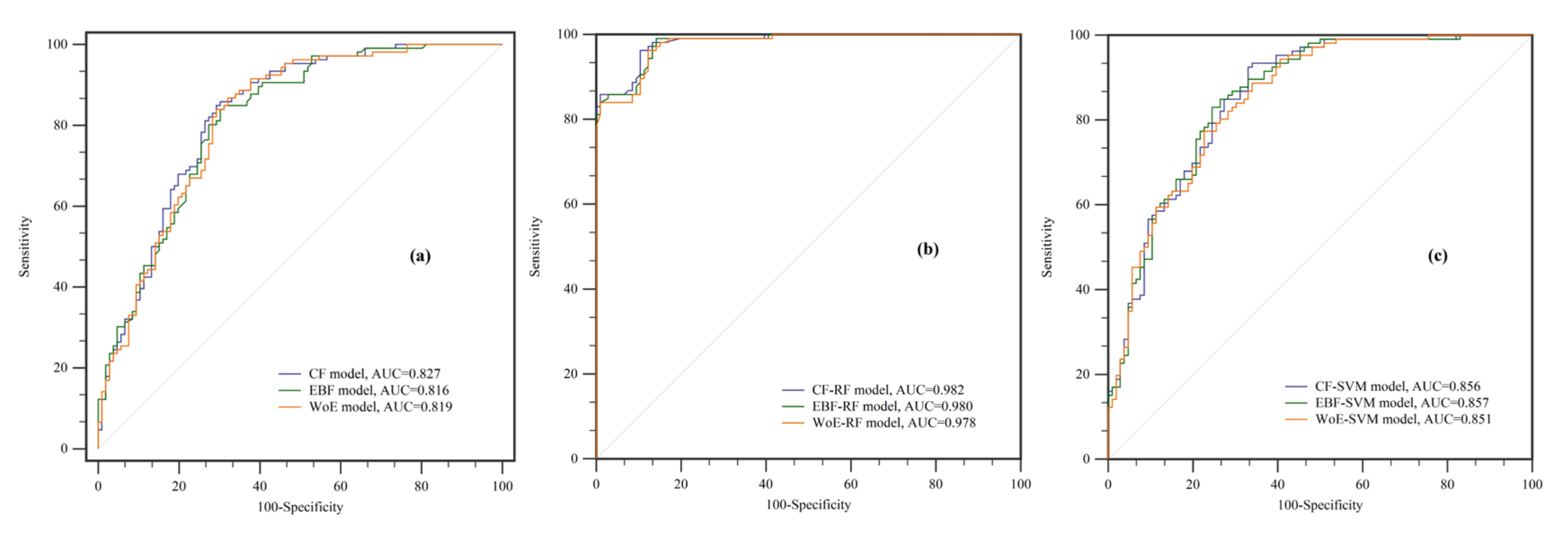
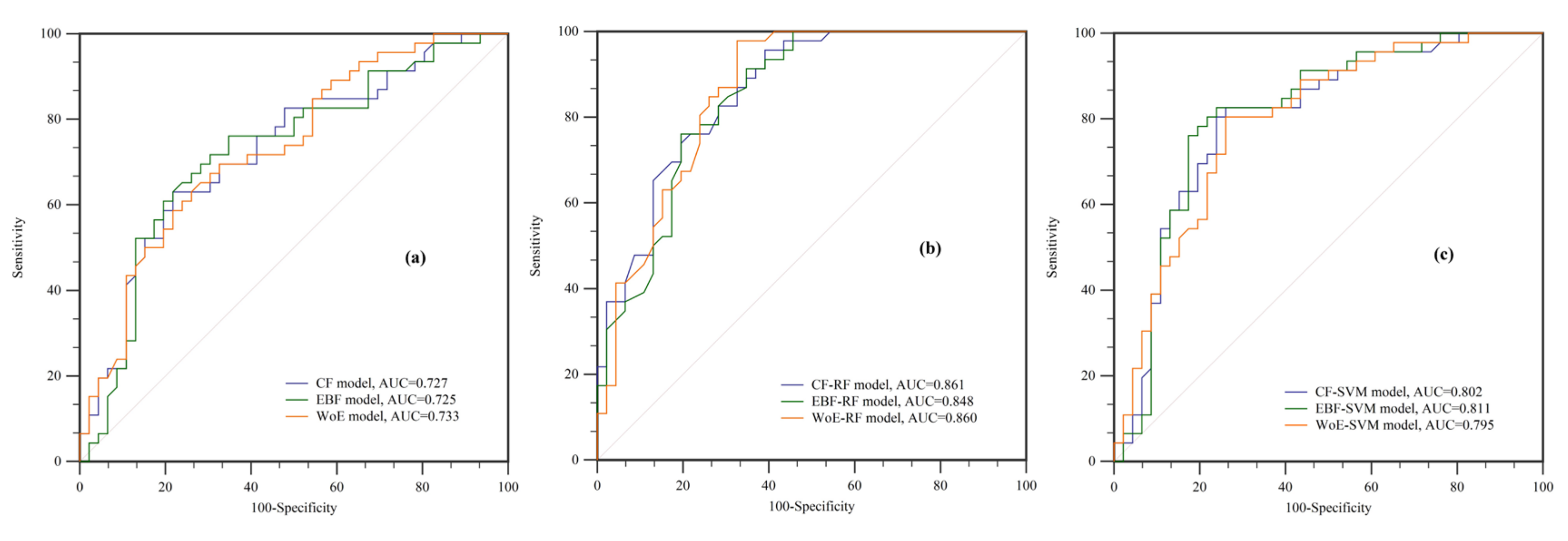
3.6. Model Validation and Comparison

In this study, the performance and prediction accuracy of the individual bivariate models and its ensembles with RF and SVM models were checked and analyzed using training and validation datasets by plotting the ROC curve [96,97,98] (

Table 1. Models performance using training dataset.

Variable	AUC	SE	95% CI
CF	0.827	0.0285	0.769 to 0.875
EBF	0.816	0.0289	0.758 to 0.866
WoE	0.819	0.0291	0.760 to 0.868
CF–RF	0.982	0.00650	0.954 to 0.995
EBF–RF	0.980	0.00696	0.951 to 0.994
WoE–RF	0.978	0.00742	0.948 to 0.993
CF–SVM	0.856	0.0256	0.802 to 0.901
EBF–SVM	0.857	0.0256	0.802 to 0.901
WoE–SVM	0.851	0.0258	0.796 to 0.896

;

Table 2. Models performance using validating dataset.

Variable	AUC	SE	95% CI
CF	0.727	0.0532	0.624 to 0.815
EBF	0.725	0.0545	0.622 to 0.813
WoE	0.733	0.0521	0.631 to 0.820
CF–RF	0.861	0.0375	0.773 to 0.924
EBF–RF	0.848	0.0402	0.758 to 0.914
WoE–RF	0.860	0.0392	0.772 to 0.924
CF–SVM	0.802	0.0476	0.706 to 0.878
EBF–SVM	0.811	0.0476	0.716 to 0.885
WoE–SVM	0.795	0.0472	0.698 to 0.872

, Figure 6 and Figure 7). The SVM was used as a benchmark model for assessing the ensemble of the bivariate models with RF classifiers. The SVM is known as a powerful state-of-the-art soft computing machine learning model that outperformed other models in many studies of susceptibility mapping [47,99]. The AUC, SE and CI at 95% confidence level statistical metrics were used for this aim. According to Table 1, results showed that the AUC values were 0.827, 0.816, 0.819, 0.982, 0.980, 0.978, 0.856, 0.856 and 0.857 for CF, EBF, WoE, CF–RF, EBF–RF, WoE–RF, CF–SVM, EBF–SVM and WoE–SVM models, respectively. According to Table 1, results showed that among individual models, the CF had the highest performance (AUC = 0.827), followed by WoE and EBF models. Moreover, it shows that among ensemble models, the highest performance was obtained for the CF–RF model, followed by EBF–RF and WoE–RF models. In other words, the bivariate models, when integrated with the RF model, had the highest performance/goodness-of-fit compared to its ensembles with the SVM model.

The results of the prediction accuracy of the individual bivariate models and its ensembles with RF and SVM using the validation dataset are shown in Table 2 and Figure 7. Although according to the training dataset, the CF bivariate model was more powerful than the EBF and WoE models, the WoE model based on the validation dataset was selected as having the highest prediction accuracy. Additionally, it indicated that the AUC values were 0.727, 0.725, 0.733, 0.861, 0.848, 0.860, 0.802, 0.811 and 0.795 for CF, EBF, WoE, CF–RF, EBF–RF, WoE–RF, CF–SVM, EBF–SVM and WoE–SVM models, respectively. It is also similar to the training dataset that of all of these models: the CF bivariate model integrated with RF model outperformed and outclassed other models with the highest prediction accuracy (AUC = 0.861). This was followed by WoE–SVM (AUC = 0.860) and EBF–SVM (AUC = 0.848). However, the individual bivariate models, when integrated with the SVM model, showed improved prediction accuracy.

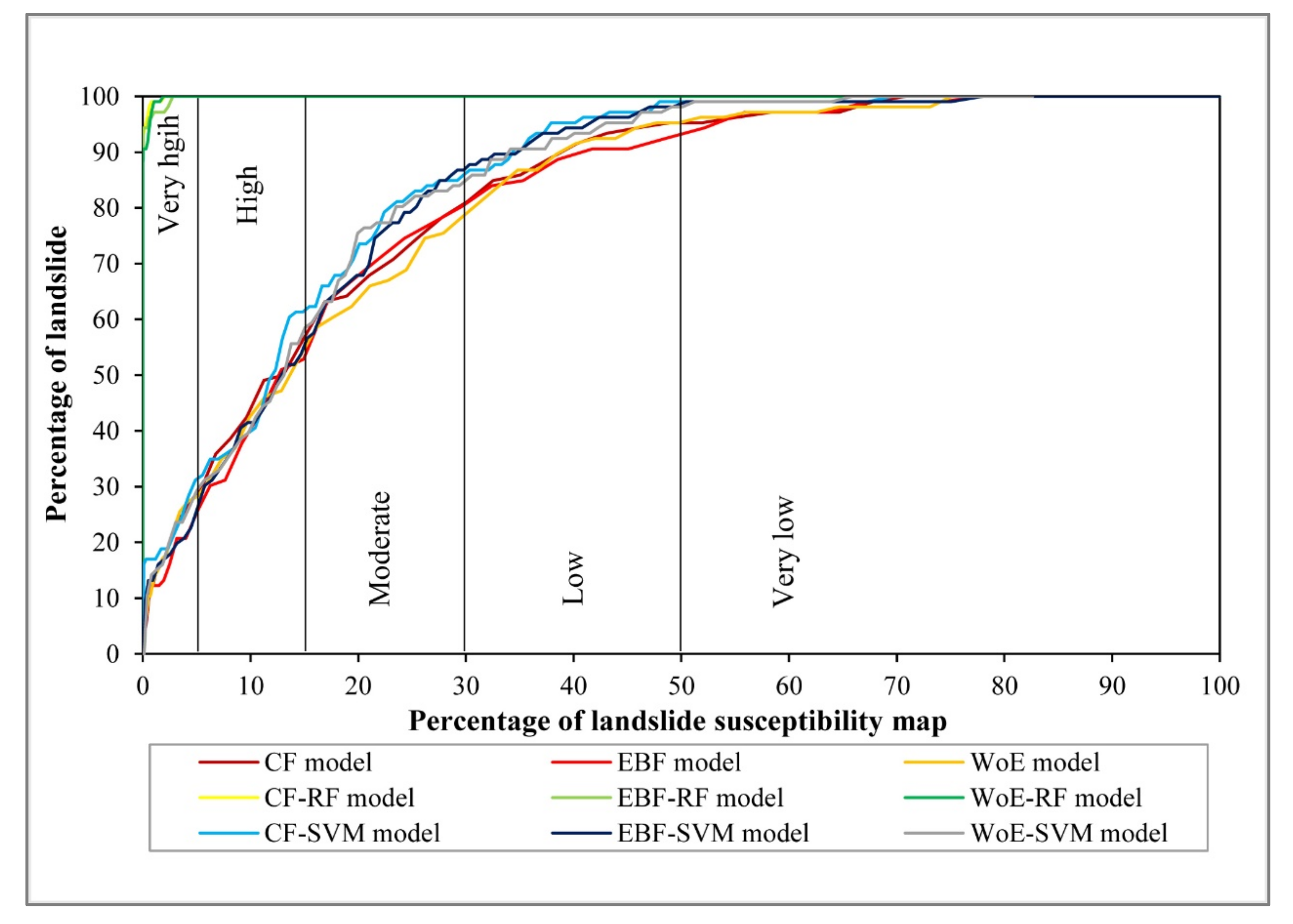
3.7. Validation of Landslide Susceptibility Maps

In this study, in addition to checking the goodness-of-fit and prediction accuracy by the ROC curve, we evaluated the usability of the proposed models using success and prediction rate curves. The ROC curve was plotted based on training and validation datasets, that are used to evaluate the performance and prediction accuracy of a given model [100,101]. However, the success and prediction rate curves were designed based on only landslide locations divided into training and validation datasets, respectively [95].

Table 3. Validation of landslide susceptibility maps.

Variable	AUC_T	AUC_P
CF	0.8324	0.7679
EBF	0.8244	0.7508
WoE	0.8251	0.7646
CF–RF	0.9996	0.8810
EBF–RF	0.9991	0.8763
WoE–RF	0.9993	0.8968
CF–SVM	0.8558	0.8105
EBF–SVM	0.8461	0.8066
WoE–SVM	0.8484	0.8055

and Figure 8 and Figure 9 show the validation of the proposed models by success (AUC_T) and prediction (AUC_P) rate curves. It can be observed that individual models had a higher performance in comparison to the ROC curve (AUC > 0.82). Among individual bivariate models, results illustrated that the CF model had the highest performance (AUC_T = 0.8324) and prediction accuracy (AUC_P = 0.7679) for landslide susceptibility mapping in the study area, followed by WoE and EBF models. Results according to training dataset showed that the AUC-Ts were 0.8324, 0.8244, 0.8251, 0.9996, 0.9991, 0.9993, 0.8558, 0.8461 and 0.8484 for CF, EBF, WoE, CF–RF, EBF–RF, WoE–RF, CF–SVM, EBF–SVM and WoE–SVM models, respectively. However, based on validation datasets, these values were 0.7679, 0.7508, 0.7646, 0.8810, 0.8763, 0.8968, 0.8105, 0.8066, and 0.8055, respectively. Overall, results based on the validation dataset indicated that WoE–RF was the accurate ensemble model (AUC_P = 0.8968). This was followed by CF–RF, EBF–RF, CF–SVM, EBF–SVM and WoE–SVM ensemble models.

4. Discussion

Landslides are one of the most significant natural disasters for all countries in the world, and landslide prediction is getting more and more attention [102]. To obtain higher accuracy of landslide susceptibility maps, there are higher requirements for the quality of the collected data, the selection of suitable models and the selection of effective parameters of the models [7]. The main advantage of the bivariate model is that it is easy to understand, does not require too much training and does not require parameter adjustment. However, bivariate algorithm modeling must be based on strict compliance with assumptions and does not analyze the relationships between each factor. Therefore, the bivariate model always ignores the importance of parameters. For machine learning models, these problems are avoided. Machine learning algorithms can determine the best parameters, but they cannot determine the weight of each factor category. It is therefore particularly necessary to introduce some integrated models to eliminate these limitations. In recent years, some integrated machine learning methods have been applied to landslide susceptibility research. For example, Nguyen et al. [103] proposed a new hybrid machine learning model for spatial prediction of landslides, namely particle swarm optimization adaptive neural fuzzy inference system (PSOANFIS), particle swarm optimization artificial neural network (PSOANN) and rotation forest based on optimal first decision tree (RFBFDT). The results showed that RFBFDT (AUC = 0.826) is the best method compared with other hybrid models and a promising hybrid machine learning method. Tien Bui et al. [104] proposed an integrated model (ABSGD) combining a function algorithm, stochastic gradient descent (SGD) and AdaBoost (AB) Meta classifier to predict the spatial distribution of landslides in Iran’s Sarkhoon watershed. The results showed that the performance of the ABSGD model (AUC = 0.860) is better than other models. The combined use of the function algorithm and the Meta classifier can reduce noise, prevent overfitting, and improve the prediction ability of a single SGD algorithm in landslide spatial prediction. Pham et al. [105] proposed a new hybrid intelligent model MBSVM for landslides in the Uttarakhand State, Northern India, which is an integration of MultiBoost integration and support vector machine (SVM). Comparison results show that MBSVM (AUC =  0.966) is superior to LR, single SVM and mixed ABSVM models.

In this article, the landslide susceptibility was simulated for 15 landslide conditioning factors such as the slope aspect, slope angle, elevation, SPI, STI, TWI, plan curvature, profile curvature, landuse, NDVI, soil, lithology, rainfall, distance to rivers and distance to roads. The CF, EBF and WoE models as bivariate models and the RF and SVM models as machine learning models were integrated and compared to choose the best model. The CF, WoE and EBF models calculated the correlation between landslide conditioning factors and landslide occurrence. The weights of the CF, EBF and WoE models are used to judge the importance of each type of factor for landslides. In order to get an integrated model with the RF model, firstly, the CF, EBF and WoE models were calculated and the LSI of various landslide conditioning factors was recorded. Then, LSI was superimposed with the landslide dataset, and the corresponding features were extracted for each landslide point in the dataset to form new model training input data. Finally, the LSI calculated by the Weka software was converted into ArcGIS software, and the landslide susceptibility map is obtained and partitioned. The same is true for the comparative SVM integration model. In order to obtain the advantages and disadvantages between the models, the ROC curve and the necessary parameters are used for comparison between the models. The comparison of the nine models shows that all the integrated models are better than all the single models, and the CF-RF model has the best performance among the nine models. The integration model mixed with RF is superior to the integration model mixed with the comparison model SVM selected after many tests. The CF–RF model in the validation data set had the largest AUC value (0.848) and the smallest SE (0.0375). In order to obtain the most suitable model for this study area more accurately, the success rate (AUC_T) curve and the prediction rate (AUC_P) curve were introduced to verify the AUC value obtained by the nine models. As stated in the results, the success rate (AUC_T) curve and the prediction rate (AUC_P) curve only consider the landslides that have occurred, and will have better performance than the AUC value obtained by the ROC curve. For the landslide susceptibility map, this classification method will be better matching. The results show that the WoE–RF model as an integrated model is superior to the other eight models (AUC_T: 0.9993, AUC_P: 0.8968). The other eight models also produced reasonable and good performance.

5. Conclusions

Landslide susceptibility prediction is critical to spatial planning and civil safety. Landslide susceptibility mapping is an indispensable step for spatial prediction of landslide susceptibility. This study introduced RF as a machine learning algorithm combined with three bivariate models (the CF, WoE and EBF models) to solve this problem. For this reason, 15 conditioning factors were selected in the study area. These factors are slope aspect, slope angle, elevation, SPI, STI, TWI, plan curvature, profile curvature, landuse, NDVI, soil, lithology, rainfall, distance to rivers and distance to roads. In this paper, the correlation between the conditioning factor and the occurrence of landslide were calculated by three different bivariate models, and the weights were obtained. Then, the weights of the bivariate model were brought into the machine learning model to form six integrated models. Next, these nine different models were applied to the spatial prediction of landslides in Linyou County. Finally, the accuracy of the generated model was verified by the ROC curve, the success rate curve and the prediction rate curve using two ways of solving the AUC value, and the best model was obtained by comparison. The AUC_T values of the CF, EBF, WoE, CF–RF, EBF–RF, WoE–RF, CF–SVM, EBF–SVM and WoE–SVM models were 0.8324, 0.8244, 0.8251, 0.9996, 0.9991, 0.9993, 0.8558, 0.8461 and 0.8484, respectively. The results show that all models have good prediction accuracy, but the prediction ability is different. After comparing the performance of the single model and the hybrid model, it was found that the performance of the single model is significantly improved after the collection. As an integrated model, the WoE–RF model has the highest prediction rate (AUC_T: 0.9993, AUC_P: 0.8968). Therefore, the nine landslide susceptibility maps produced by Linyou County can be used as useful tools for government personnel and local authorities to carry out land management and planning.

References

1. Gutierrez, F.; Linares, R.; Roque, C.; Zarroca, M.; Carbonel, D.; Rosell, J.; Gutierrez, M. Large landslides associated with a diapiric fold in canelles reservoir (Spanish pyrenees): Detailed geological-geomorphological mapping, trenching and electrical resistivity imaging. Geomorphology 2015, 241, 224–242. [Google Scholar] [CrossRef]
2. Komac, M.; Hribernik, K. Slovenian national landslide database as a basis for statistical assessment of landslide phenomena in Slovenia. Geomorphology 2015, 249, 94–102. [Google Scholar] [CrossRef]
3. Guzzetti, F.; Reichenbach, P.; Ardizzone, F.; Cardinali, M.; Galli, M. Estimating the quality of landslide susceptibility models. Geomorphology 2006, 81, 166–184. [Google Scholar] [CrossRef]
4. Raja, N.B.; Cicek, I.; Turkoglu, N.; Aydin, O.; Kawasaki, A. Landslide susceptibility mapping of the Sera River Basin using logistic regression model. Nat. Hazards 2017, 85, 1323–1346. [Google Scholar] [CrossRef] [Green Version]
5. Sema, H.V.; Guru, B.; Veerappan, R. Fuzzy gamma operator model for preparing landslide susceptibility zonation mapping in parts of Kohima Town, Nagaland, India. Modeling Earth Syst. Environ. 2017, 3, 499–514. [Google Scholar] [CrossRef]
6. Chen, W.; Fan, L.; Li, C.; Pham, B.T. Spatial prediction of landslides using hybrid integration of artificial intelligence algorithms with frequency ratio and index of entropy in Nanzheng county, China. Appl. Sci. 2020, 10, 29. [Google Scholar] [CrossRef] [Green Version]
7. Ayalew, L.; Yamagishi, H. The application of GIS-based logistic regression for landslide susceptibility mapping in the Kakuda-Yahiko Mountains, Central Japan. Geomorphology 2005, 65, 15–31. [Google Scholar] [CrossRef]
8. Balamurugan, G.; Ramesh, V.; Touthang, M. Landslide susceptibility zonation mapping using frequency ratio and fuzzy gamma operator models in part of NH-39, Manipur, India. Nat. Hazards 2016, 84, 465–488. [Google Scholar] [CrossRef]
9. Nhu, V.-H.; Mohammadi, A.; Shahabi, H.; Ahmad, B.B.; Al-Ansari, N.; Shirzadi, A.; Clague, J.J.; Jaafari, A.; Chen, W.; Nguyen, H. Landslide susceptibility mapping using machine learning algorithms and remote sensing data in a tropical environment. Int. J. Environ. Res. Public Health 2020, 17, 4933. [Google Scholar] [CrossRef]
10. Lacasse, S.; Nadim, F.; Lacasse, S.; Nadim, F. Landslide Risk Assessment and Mitigation Strategy. In Landslides–Disaster Risk Reduction; Springer: Berlin/Heidelberg, Germany, 2009; pp. 31–61. [Google Scholar]
11. Zhao, X.; Chen, W. Optimization of Computational Intelligence Models for Landslide Susceptibility Evaluation. Remote Sens. 2020, 12, 2180. [Google Scholar] [CrossRef]
12. Chen, W.; Pourghasemi, H.R.; Kornejady, A.; Zhang, N. Landslide spatial modeling: Introducing new ensembles of ANN, MaxEnt, and SVM machine learning techniques. Geoderma 2017, 305, 314–327. [Google Scholar] [CrossRef]
13. Chen, W.; Zhao, X.; Shahabi, H.; Shirzadi, A.; Khosravi, K.; Chai, H.; Zhang, S.; Zhang, L.; Ma, J.; Chen, Y.; et al. Spatial prediction of landslide susceptibility by combining evidential belief function, logistic regression and logistic model tree. Geocarto Int. 2019, 34, 1177–1201. [Google Scholar] [CrossRef]
14. Mandal, S.; Maiti, R. Application of Analytical Hierarchy Process (AHP) and Frequency Ratio (FR) Model in Assessing Landslide Susceptibility and Risk. In Semi-quantitative Approaches for Landslide Assessment and Prediction; Springer: Singapore, 2015; pp. 191–226. [Google Scholar]
15. Pourghasemi, H.R.; Pradhan, B.; Gokceoglu, C. Application of fuzzy logic and analytical hierarchy process (AHP) to landslide susceptibility mapping at Haraz watershed, Iran. Nat. Hazards 2012, 63, 965–996. [Google Scholar] [CrossRef]
16. Chen, W.; Li, W.; Chai, H.; Hou, E.; Li, X.; Ding, X. GIS-based landslide susceptibility mapping using analytical hierarchy process (AHP) and certainty factor (CF) models for the Baozhong region of Baoji City, China. Environ. Earth Sci. 2015, 75, 63. [Google Scholar] [CrossRef]
17. Jie, D.; Oguchi, T.; Hayakawa, Y.S.; Uchiyama, S.; Saito, H.; Paudel, U. GIS-Based Landslide Susceptibility Mapping Using a Certainty Factor Model and Its Validation in the Chuetsu Area, Central Japan. In Landslide Science for a Safer Geoenvironment; Springer: Cham, Switzerland, 2014. [Google Scholar]
18. Pourghasemi, H.R.; Kerle, N. Random forests and evidential belief function-based landslide susceptibility assessment in Western Mazandaran Province, Iran. Environ. Earth Sci. 2016, 75, 185. [Google Scholar] [CrossRef]
19. Shahabi, H.; Hashim, M.; Ahmad, B.B. Remote sensing and GIS-based landslide susceptibility mapping using frequency ratio, logistic regression, and fuzzy logic methods at the central Zab basin, Iran. Environ. Earth Sci. 2015, 73, 8647–8668. [Google Scholar] [CrossRef]
20. Wang, L.-J.; Guo, M.; Sawada, K.; Lin, J.; Zhang, J. A comparative study of landslide susceptibility maps using logistic regression, frequency ratio, decision tree, weights of evidence and artificial neural network. Geosci. J. 2015, 20, 117–136. [Google Scholar] [CrossRef]
21. Youssef, A.M.; Al-Kathery, M.; Pradhan, B. Landslide susceptibility mapping at Al-Hasher area, Jizan (Saudi Arabia) using GIS-based frequency ratio and index of entropy models. Geosci. J. 2014, 19, 113–134. [Google Scholar] [CrossRef]
22. Wang, G.; Lei, X.; Chen, W.; Shahabi, H.; Shirzadi, A. Hybrid Computational Intelligence Methods for Landslide Susceptibility Mapping. Symmetry 2020, 12, 325. [Google Scholar] [CrossRef] [Green Version]
23. Peng, L.; Niu, R.; Huang, B.; Wu, X.; Zhao, Y.; Ye, R. Landslide susceptibility mapping based on rough set theory and support vector machines: A case of the Three Gorges area, China. Geomorphology 2014, 204, 287–301. [Google Scholar] [CrossRef]
24. Chen, W.; Chai, H.; Zhao, Z.; Wang, Q.; Hong, H. Landslide susceptibility mapping based on GIS and support vector machine models for the Qianyang County, China. Environ. Earth Sci. 2016, 75, 474. [Google Scholar] [CrossRef]
25. Zhou, S.; Fang, L. Support vector machine modeling of earthquake-induced landslides susceptibility in central part of Sichuan province, China. Geoenviron. Disasters 2015, 2, 2. [Google Scholar] [CrossRef] [Green Version]
26. Nhu, V.-H.; Shirzadi, A.; Shahabi, H.; Singh, S.K.; Al-Ansari, N.; Clague, J.J.; Jaafari, A.; Chen, W.; Miraki, S.; Dou, J. Shallow Landslide Susceptibility Mapping: A Comparison between Logistic Model Tree, Logistic Regression, Na ve Bayes Tree, Artificial Neural Network, and Support Vector Machine Algorithms. Int. J. Environ. Res. Public Health 2020, 17, 2749. [Google Scholar] [CrossRef] [PubMed]
27. Stumpf, A.; Kerle, N. Object-oriented mapping of landslides using Random Forests. Remote Sens. Environ. 2011, 115, 2564–2577. [Google Scholar] [CrossRef]
28. Chen, W.; Li, X.; Wang, Y.; Chen, G.; Liu, S. Forested landslide detection using LiDAR data and the random forest algorithm: A case study of the Three Gorges, China. Remote Sens. Environ. 2014, 152, 291–301. [Google Scholar] [CrossRef]
29. Shafizadeh-Moghadam, H.; Minaei, M.; Shahabi, H.; Hagenauer, J. Big data in geohazard; pattern mining and large scale analysis of landslides in Iran. Earth Sci. Inform. 2019, 12, 1–17. [Google Scholar] [CrossRef]
30. Polykretis, C.; Ferentinou, M.; Chalkias, C. A comparative study of landslide susceptibility mapping using landslide susceptibility index and artificial neural networks in the Krios River and Krathis River catchments (northern Peloponnesus, Greece). Bull. Eng. Geol. Environ. 2014, 74, 27–45. [Google Scholar] [CrossRef]
31. Lian, C.; Zeng, Z.; Yao, W.; Tang, H. Multiple neural networks switched prediction for landslide displacement. Eng. Geol. 2015, 186, 91–99. [Google Scholar] [CrossRef]
32. Gelisli, K.; Kaya, T.; Babacan, A.E. Assessing the factor of safety using an artificial neural network: Case studies on landslides in Giresun, Turkey. Environ. Earth Sci. 2015, 73, 8639–8646. [Google Scholar] [CrossRef]
33. Arnone, E.; Francipane, A.; Noto, L.V.; Scarbaci, A.; La Loggia, G. Strategies investigation in using artificial neural network for landslide susceptibility mapping: Application to a Sicilian catchment. J. Hydroinform. 2014, 16, 502–515. [Google Scholar] [CrossRef]
34. Tsai, F.; Lai, J.-S.; Chen, W.W.; Lin, T.-H. Analysis of topographic and vegetative factors with data mining for landslide verification. Ecol. Eng. 2013, 61, 669–677. [Google Scholar] [CrossRef]
35. Yeon, Y.-K.; Han, J.-G.; Ryu, K.H. Landslide susceptibility mapping in Injae, Korea, using a decision tree. Eng. Geol. 2010, 116, 274–283. [Google Scholar] [CrossRef]
36. Marjanović, M.; Kovačević, M.; Bajat, B.; Voženílek, V. Landslide susceptibility assessment using SVM machine learning algorithm. Eng. Geol. 2011, 123, 225–234. [Google Scholar] [CrossRef]
37. Althuwaynee, O.F.; Pradhan, B.; Park, H.-J.; Lee, J.H. A novel ensemble decision tree-based CHi-squared Automatic Interaction Detection (CHAID) and multivariate logistic regression models in landslide susceptibility mapping. Landslides 2014, 11, 1063–1078. [Google Scholar] [CrossRef]
38. Felicísimo, Á.M.; Cuartero, A.; Remondo, J.; Quirós, E. Mapping landslide susceptibility with logistic regression, multiple adaptive regression splines, classification and regression trees, and maximum entropy methods: A comparative study. Landslides 2012, 10, 175–189. [Google Scholar] [CrossRef]
39. Li, Y.; Chen, W. Landslide Susceptibility Evaluation Using Hybrid Integration of Evidential Belief Function and Machine Learning Techniques. Water 2020, 12, 113. [Google Scholar] [CrossRef] [Green Version]
40. Park, N.-W. Using maximum entropy modeling for landslide susceptibility mapping with multiple geoenvironmental data sets. Environ. Earth Sci. 2014, 73, 937–949. [Google Scholar] [CrossRef]
41. Kim, H.G.; Lee, D.K.; Park, C.; Kil, S.; Son, Y.; Park, J.H. Evaluating landslide hazards using RCP 4.5 and 8.5 scenarios. Environ. Earth Sci. 2014, 73, 1385–1400. [Google Scholar] [CrossRef]
42. Davis, J.; Blesius, L. A Hybrid Physical and Maximum-Entropy Landslide Susceptibility Model. Entropy 2015, 17, 4271–4292. [Google Scholar] [CrossRef] [Green Version]
43. Tsangaratos, P.; Ilia, I. Comparison of a logistic regression and Naïve Bayes classifier in landslide susceptibility assessments: The influence of models complexity and training dataset size. Catena 2016, 145, 164–179. [Google Scholar] [CrossRef]
44. Oh, H.-J.; Pradhan, B. Application of a neuro-fuzzy model to landslide-susceptibility mapping for shallow landslides in a tropical hilly area. Comput. Geosci. 2011, 37, 1264–1276. [Google Scholar] [CrossRef]
45. Chen, W.; Chen, X.; Peng, J.; Panahi, M.; Lee, S. Landslide susceptibility modeling based on ANFIS with teaching-learning-based optimization and Satin bowerbird optimizer. Geosci. Front. 2021, 12, 93–107. [Google Scholar] [CrossRef]
46. Chen, X.; Chen, W. GIS-based landslide susceptibility assessment using optimized hybrid machine learning methods. CATENA 2021, 196, 104833. [Google Scholar] [CrossRef]
47. Tien Bui, D.; Tuan, T.A.; Klempe, H.; Pradhan, B.; Revhaug, I. Spatial prediction models for shallow landslide hazards: A comparative assessment of the efficacy of support vector machines, artificial neural networks, kernel logistic regression, and logistic model tree. Landslides 2016, 13, 361–378. [Google Scholar] [CrossRef]
48. Pham, B.T.; Tien Bui, D.; Prakash, I. Landslide Susceptibility Assessment Using Bagging Ensemble Based Alternating Decision Trees, Logistic Regression and J48 Decision Trees Methods: A Comparative Study. Geotech. Geol. Eng. 2017, 35, 2597–2611. [Google Scholar] [CrossRef]
49. Pham, B.T.; Tien Bui, D.; Dholakia, M.B.; Prakash, I.; Pham, H.V. A Comparative Study of Least Square Support Vector Machines and Multiclass Alternating Decision Trees for Spatial Prediction of Rainfall-Induced Landslides in a Tropical Cyclones Area. Geotech. Geol. Eng. 2016, 34, 1807–1824. [Google Scholar] [CrossRef]
50. Nhu, V.-H.; Zandi, D.; Shahabi, H.; Chapi, K.; Shirzadi, A.; Al-Ansari, N.; Singh, S.K.; Dou, J.; Nguyen, H. Comparison of Support Vector Machine, Bayesian Logistic Regression, and Alternating Decision Tree Algorithms for Shallow Landslide Susceptibility Mapping along a Mountainous Road in the West of Iran. Appl. Sci. 2020, 10, 5047. [Google Scholar] [CrossRef]
51. Vorpahl, P.; Elsenbeer, H.; Märker, M.; Schröder, B. How can statistical models help to determine driving factors of landslides? Ecol. Model. 2012, 239, 27–39. [Google Scholar] [CrossRef]
52. Pham, B.T.; Shirzadi, A.; Tien Bui, D.; Prakash, I.; Dholakia, M.B. A hybrid machine learning ensemble approach based on a Radial Basis Function neural network and Rotation Forest for landslide susceptibility modeling: A case study in the Himalayan area, India. Int. J. Sediment Res. 2018, 33, 157–170. [Google Scholar] [CrossRef]
53. Chen, W.; Hong, H.; Panahi, M.; Shahabi, H.; Wang, Y.; Shirzadi, A.; Pirasteh, S.; Alesheikh, A.A.; Khosravi, K.; Panahi, S.; et al. Spatial Prediction of Landslide Susceptibility Using GIS-Based Data Mining Techniques of ANFIS with Whale Optimization Algorithm (WOA) and Grey Wolf Optimizer (GWO). Appl. Sci. 2019, 9, 3755. [Google Scholar] [CrossRef] [Green Version]
54. Althuwaynee, O.F.; Pradhan, B.; Lee, S. A novel integrated model for assessing landslide susceptibility mapping using CHAID and AHP pair-wise comparison. Int. J. Remote Sens. 2016, 37, 1190–1209. [Google Scholar] [CrossRef]
55. Bui, D.T.; Shirzadi, A.; Shahabi, H.; Geertsema, M.; Omidvar, E.; Clague, J.J.; Pham, B.T.; Dou, J.; Asl, D.T.; Ahmad, B.B. New ensemble models for shallow landslide susceptibility modeling in a semi-arid watershed. Forests 2019, 10, 743. [Google Scholar]
56. Umar, Z.; Pradhan, B.; Ahmad, A.; Jebur, M.N.; Tehrany, M.S. Earthquake induced landslide susceptibility mapping using an integrated ensemble frequency ratio and logistic regression models in West Sumatera Province, Indonesia. Catena 2014, 118, 124–135. [Google Scholar] [CrossRef]
57. Chen, W.; Xie, X.; Peng, J.; Shahabi, H.; Hong, H.; Bui, D.T.; Duan, Z.; Li, S.; Zhu, A.-X. GIS-based landslide susceptibility evaluation using a novel hybrid integration approach of bivariate statistical based random forest method. Catena 2018, 164, 135–149. [Google Scholar] [CrossRef]
58. Conforti, M.; Muto, F.; Rago, V.; Critelli, S. Landslide inventory map of north-eastern Calabria (South Italy). J. Maps 2014, 10, 90–102. [Google Scholar] [CrossRef]
59. Chen, W.; Li, Y. GIS-based evaluation of landslide susceptibility using hybrid computational intelligence models. Catena 2020, 195, 104777. [Google Scholar] [CrossRef]
60. Lei, X.; Chen, W.; Pham, B.T. Performance Evaluation of GIS-Based Artificial Intelligence Approaches for Landslide Susceptibility Modeling and Spatial Patterns Analysis. ISPRS Int. J. Geo-Inf. 2020, 9, 443. [Google Scholar] [CrossRef]
61. He, Q.; Xu, Z.; Li, S.; Li, R.; Zhang, S.; Wang, N.; Pham, B.T.; Chen, W. Novel Entropy and Rotation Forest-Based Credal Decision Tree Classifier for Landslide Susceptibility Modeling. Entropy 2019, 21, 106. [Google Scholar] [CrossRef] [Green Version]
62. Pham, B.T.; Prakash, I.; Singh, S.K.; Shirzadi, A.; Shahabi, H.; Tran, T.-T.-T.; Bui, D.T. Landslide susceptibility modeling using Reduced Error Pruning Trees and different ensemble techniques: Hybrid machine learning approaches. Catena 2019, 175, 203–218. [Google Scholar] [CrossRef]
63. Guo, C.; Montgomery, D.R.; Zhang, Y.; Wang, K.; Yang, Z. Quantitative assessment of landslide susceptibility along the Xianshuihe fault zone, Tibetan Plateau, China. Geomorphology 2015, 248, 93–110. [Google Scholar] [CrossRef]
64. Pradhan, A.M.S.; Kim, Y.T. Relative effect method of landslide susceptibility zonation in weathered granite soil: A case study in Deokjeok-ri Creek, South Korea. Nat. Hazards 2014, 72, 1189–1217. [Google Scholar] [CrossRef]
65. Moore, I.D.; Grayson, R.B.; Ladson, A.R. Digital terrain modelling: A review of hydrological, geomorphological, and biological applications. Hydrol. Process. 1991, 5, 3–30. [Google Scholar] [CrossRef]
66. Moore, I.D.; Burch, G.J. Physical Basis of the Length-slope Factor in the Universal Soil Loss Equation. Soil Sci. Soc. Am. J. 1986, 50, 1294–1298. [Google Scholar] [CrossRef]
67. Sambasivarao, K.V. Quantifying the Role of Vegetation in Slope Stability. Surg. Neurol. 2015, 4, 127–132. [Google Scholar]
68. Schwarz, M.; Preti, F.; Giadrossich, F.; Lehmann, P.; Or, D. Quantifying the role of vegetation in slope stability: A case study in Tuscany (Italy). Ecol. Eng. 2010, 36, 285–291. [Google Scholar] [CrossRef]
69. Alvioli, M.; Guzzetti, F.; Rossi, M. Scaling properties of rainfall induced landslides predicted by a physically based model. Geomorphol. Amst. 2014, 213, 38–47. [Google Scholar] [CrossRef] [Green Version]
70. Jiang, J.W.; Xiang, W.; Rohn, J.; Zeng, W.; Schleier, M. Research on water-rock (soil) interaction by dynamic tracing method for Huangtupo landslide, Three Gorges Reservoir, PR China. Environ. Earth Sci. 2015, 74, 557–571. [Google Scholar] [CrossRef]
71. Du, G.-L.; Zhang, Y.-S.; Iqbal, J.; Yang, Z.-H.; Yao, X. Landslide susceptibility mapping using an integrated model of information value method and logistic regression in the Bailongjiang watershed, Gansu Province, China. J. Mt. Sci. 2017, 14, 249–268. [Google Scholar] [CrossRef]
72. Duc, D.M. Rainfall-triggered large landslides on 15 December 2005 in Van Canh District, Binh Dinh Province, Vietnam. Landslides 2013, 10, 219–230. [Google Scholar] [CrossRef] [Green Version]
73. Pham, B.T.; Bui, D.T.; Dholakia, M.B.; Prakash, I.; Pham, H.V.; Mehmood, K.; Le, H.Q. A novel ensemble classifier of rotation forest and Naïve Bayer for landslide susceptibility assessment at the Luc Yen district, Yen Bai Province (Viet Nam) using GIS. Geomat. Nat. Hazards Risk 2017, 8, 649–671. [Google Scholar] [CrossRef] [Green Version]
74. Yalcin, A. GIS-based landslide susceptibility mapping using analytical hierarchy process and bivariate statistics in Ardesen (Turkey): Comparisons of results and confirmations. Catena 2008, 72, 1–12. [Google Scholar] [CrossRef]
75. Wang, G.; Chen, X.; Chen, W. Spatial prediction of landslide susceptibility based on gis and discriminant functions. ISPRS Int. J. Geo-Inf. 2020, 9, 144. [Google Scholar]
76. Pachauri, A.K.; Gupta, P.V.; Chander, R. Landslide zoning in a part of the Garhwal Himalayas. Environ. Geol. 1998, 36, 325–334. [Google Scholar] [CrossRef]
77. Shortliffe, E.H.; Buchanan, B.G. A model of inexact reasoning in medicine. Math. Biosci. 1990, 23, 351–379. [Google Scholar] [CrossRef]
78. Heckerman, D. Probabilistic Interpretations for MYCIN’s Certainty Factors. In Machine Intelligence and Pattern Recognition; Elsevier: North-Holland, The Netherlands, 1990; Volume 4, pp. 167–196. [Google Scholar]
79. Lan, H.X.; Zhou, C.H.; Wang, L.J.; Zhang, H.Y.; Li, R.H. Landslide hazard spatial analysis and prediction using GIS in the Xiaojiang watershed, Yunnan, China. Eng. Geol. 2004, 76, 109–128. [Google Scholar] [CrossRef]
80. Bonhamcarter, G. Geographic Information Systems for Geoscientists: Modelling with GIS; Computer Methods in the Geosciences; Elsevier: Amsterdam, The Netherlands, 1994; Volume 4, pp. 1–2. [Google Scholar]
81. Yalcin, A.; Reis, S.; Aydinoglu, A.C.; Yomralioglu, T. A GIS-based comparative study of frequency ratio, analytical hierarchy process, bivariate statistics and logistics regression methods for landslide susceptibility mapping in Trabzon, NE Turkey. Catena 2011, 85, 274–287. [Google Scholar] [CrossRef]
82. Dahal, R.K.; Hasegawa, S.; Nonomura, A.; Yamanaka, M.; Dhakal, S.; Paudyal, P. Predictive modelling of rainfall-induced landslide hazard in the Lesser Himalaya of Nepal based on weights-of-evidence. Geomo 2008, 102, 496–510. [Google Scholar] [CrossRef]
83. Shafer, G. A Theory of Statistical Evidence. In Foundations of Probability Theory, Statistical Inference, and Statistical Theories of Science; Springer: Dordrecht, The Netherlands, 1976. [Google Scholar]
84. Althuwaynee, O.F.; Pradhan, B.; Lee, S. Application of an evidential belief function model in landslide susceptibility mapping. Comput. Geosci. 2012, 44, 120–135. [Google Scholar] [CrossRef]
85. Lee, S.; Hwang, J.; Park, I. Application of data-driven evidential belief functions to landslide susceptibility mapping in Jinbu, Korea. Catena 2013, 100, 15–30. [Google Scholar] [CrossRef]
86. Breiman, L. Random Forests. Mach. Learn. 2001, 45, 5–32. [Google Scholar] [CrossRef] [Green Version]
87. Calderoni, L.; Ferrara, M.; Franco, A.; Maio, D. Indoor localization in a hospital environment using Random Forest classifiers. Expert Syst. Appl. 2015, 42, 125–134. [Google Scholar] [CrossRef]
88. Khanna, P.K.; Madeira, M.; Fabiao, A. Sustainability and forest soils. Forest Ecol. Manag. 2002, 171, 1–2. [Google Scholar] [CrossRef]
89. Masetic, Z.; Subasi, A. Congestive heart failure detection using random forest classifier. Comput. Methods Programs Biomed. 2016, 130, 54–64. [Google Scholar] [CrossRef] [PubMed]
90. Chen, W.; Pourghasemi, H.R.; Panahi, M.; Kornejady, A.; Wang, J.; Xie, X.; Cao, S. Spatial prediction of landslide susceptibility using an adaptive neuro-fuzzy inference system combined with frequency ratio, generalized additive model, and support vector machine techniques. Geomorphology 2017, 297, 69–85. [Google Scholar] [CrossRef]
91. Pourghasemi, H.R.; Jirandeh, A.G.; Pradhan, B.; Chong, X.U.; Gokceoglu, C. Landslide susceptibility mapping using support vector machine and GIS at the Golestan Province, Iran. J. Earth Syst. Sci. 2013, 122, 349–369. [Google Scholar] [CrossRef] [Green Version]
92. Vapnik, V.N. Controlling the Generalization Ability of Learning Processes. In The Nature of Statistical Learning Theory; Springer: New York, NY, USA, 1995. [Google Scholar]
93. Feizizadeh, B.; Roodposhti, M.S.; Blaschke, T.; Aryal, J. Comparing GIS-based support vector machine kernel functions for landslide susceptibility mapping. Arab. J. Geosci. 2017, 10, 122. [Google Scholar] [CrossRef]
94. Frank, E.; Hall, A.M.; Witten, H.I. The Weka Workbench. Online Appendix for "Data Mining: Practical Machine Learning Tools and Techniques", 4th ed.; Morgan Kaufmann: Burlington, MA, USA, 2016. [Google Scholar]
95. Chen, W.; Shahabi, H.; Shirzadi, A.; Hong, H.; Akgun, A.; Tian, Y.; Liu, J.; Zhu, A.X.; Li, S. Novel hybrid artificial intelligence approach of bivariate statistical-methods-based kernel logistic regression classifier for landslide susceptibility modeling. Bull. Eng. Geol. Environ. 2019, 78, 4397–4419. [Google Scholar] [CrossRef]
96. Lei, X.; Chen, W.; Avand, M.; Janizadeh, S.; Kariminejad, N.; Shahabi, H.; Costache, R.; Shahabi, H.; Shirzadi, A.; Mosavi, A. GIS-Based Machine Learning Algorithms for Gully Erosion Susceptibility Mapping in a Semi-Arid Region of Iran. Remote Sens. 2020, 12, 2478. [Google Scholar] [CrossRef]
97. Zhao, X.; Chen, W. GIS-Based Evaluation of Landslide Susceptibility Models Using Certainty Factors and Functional Trees-Based Ensemble Techniques. Appl. Sci. 2020, 10, 16. [Google Scholar] [CrossRef] [Green Version]
98. Nhu, V.-H.; Shirzadi, A.; Shahabi, H.; Chen, W.; Clague, J.J.; Geertsema, M.; Jaafari, A.; Avand, M.; Miraki, S.; Talebpour Asl, D. Shallow landslide susceptibility mapping by random forest base classifier and its ensembles in a semi-arid region of Iran. Forests 2020, 11, 421. [Google Scholar] [CrossRef] [Green Version]
99. Abedini, M.; Ghasemian, B.; Shirzadi, A.; Bui, D.T. A comparative study of support vector machine and logistic model tree classifiers for shallow landslide susceptibility modeling. Environ. Earth Sci. 2019, 78, 560. [Google Scholar] [CrossRef]
100. Chen, W.; Zhao, X.; Tsangaratos, P.; Shahabi, H.; Ilia, I.; Xue, W.; Wang, X.; Ahmad, B.B. Evaluating the usage of tree-based ensemble methods in groundwater spring potential mapping. J. Hydrol. 2020, 583, 124602. [Google Scholar] [CrossRef]
101. Nhu, V.-H.; Mohammadi, A.; Shahabi, H.; Ahmad, B.B.; Al-Ansari, N.; Shirzadi, A.; Geertsema, M.; Kress, V.R.; Karimzadeh, S.; Kamran, K.V. Landslide Detection and Susceptibility Modeling on Cameron Highlands (Malaysia): A Comparison between Random Forest, Logistic Regression and Logistic Model Tree Algorithms. Forests 2020, 11, 830. [Google Scholar] [CrossRef]
102. Pham, B.T.; Tien Bui, D.; Pourghasemi, H.R.; Indra, P.; Dholakia, M.B. Landslide susceptibility assesssment in the Uttarakhand area (India) using GIS: A comparison study of prediction capability of naïve bayes, multilayer perceptron neural networks, and functional trees methods. Theor. Appl. Climatol. 2017, 128, 255–273. [Google Scholar] [CrossRef]
103. Nguyen, V.; Pham, B.; Vu, B.; Prakash, I.; Jha, S.; Shahabi, H.; Shirzadi, A.; Ba, D.; Kumar, R.; Chatterjee, J. Hybrid Machine Learning Approaches for Landslide Susceptibility Modeling. Forests 2019, 10, 157. [Google Scholar] [CrossRef] [Green Version]
104. Tien Bui, D.; Shahabi, H.; Omidvar, E.; Shirzadi, A.; Geertsema, M.; Clague, J.; Khosravi, K.; Pradhan, B.; Pham, B.; Chapi, K.; et al. Shallow Landslide Prediction Using a Novel Hybrid Functional Machine Learning Algorithm. Remote Sens. 2019, 11, 931. [Google Scholar] [CrossRef] [Green Version]
105. Pham, B.T.; Jaafari, A.; Prakash, I.; Bui, D.T. A novel hybrid intelligent model of support vector machines and the MultiBoost ensemble for landslide susceptibility modeling. Bull. Eng. Geol. Environ. 2019, 78, 2865–2886. [Google Scholar] [CrossRef]
Figure 1. Location of the study area.
Ijgi 09 00696 g001
Figure 2. Rainfall distribution from 1990 to 2019.
Ijgi 09 00696 g002
Figure 3. Maps of landslide conditioning factors: (a) slope aspect; (b) slope angle; (c) elevation; (d) stream power index (SPI); (e) sediment transport index (STI); (f) topographic wetness index (TWI); (g) plan curvature; (h) profile curvature; (i) land use; (j) normalized difference vegetation index (NDVI); (k) soil; (l) lithology; (m) rainfall; (n) distance to rivers; (o) distance to roads.
Ijgi 09 00696 g003
Figure 4. Weights of factors using certainty factors (CFs), evidential belief function (EBF) and weights of evidence (WoE) models.
Ijgi 09 00696 g004
Figure 5. Landslide susceptibility maps: (a) CF model, (b) EBF model, (c) WoE model, (d) CF-RF model, (e) EBF–RF model, (f) WoE–RF model, (g) CF–SVM model, (h) EBF–SVM model, (i) WoE–SVM model.
Ijgi 09 00696 g005
Figure 6. ROC curves using training data. Performance and prediction accuracy of the individual bivariate models (a) and its ensembles with RF (b) and SVM (c) models.
Ijgi 09 00696 g006
Figure 7. ROC curves using validating data. Performance and prediction accuracy of the individual bivariate models (a) and its ensembles with RF (b) and SVM (c) models.
Ijgi 09 00696 g007
Figure 8. Model validation with the success rate (AUC_T) curve.
Ijgi 09 00696 g008
Figure 9. Model validation with the prediction rate (AUC_P) curve.
Ijgi 09 00696 g009