1. Introduction
Condition assessment is a fundamental phase in conservation projects of historic buildings and sites [
1]. It can be considered as part of the process for planning future interventions on historic buildings, and has a strong connection to the geometric survey with traditional and modern surveying techniques.
Laser scanning technology and digital photogrammetry can provide a detailed set of measured drawings in CAD (computer-aided design) formats (such as plans, sections, and elevations), advanced 3D models based on pure geometry, or parametric models like historic building information modeling (HBIM) [
2]. Nowadays, photogrammetry [
3] and laser scanning [
4] are the best solutions available to record the geometry of historic buildings and sites. The use of dense point clouds provides all the information to capture surfaces and their irregularities, such as variable thickness or deviations from verticality. However, the geometric survey does not give information about construction materials and their conditions, which could have an ongoing degradation caused by a combination of pathologies.
Recording construction technologies, materials, and their conditions is part of the workflow of a complete restoration project. The technical drawings form the base where such information will be recorded. For instance, the different pathologies found on a façade could be represented in an elevation using hatches, symbols, and colors. A legend explains the meaning of each symbol, such as in the example shown in
Figure 1.
In recent years, the advancements in digital tools for the geometric survey have provided new deliverables where material and decay information is recorded [
5]. Accurate visual supports, such as rectified images or CAD drawings, are the most popular solutions adopted by the expert in conservation. Nowadays, the most used solution to document conditions on flat surfaces (e.g., walls, floors, building facades) is rectified photography. An image (or a set of images) is rectified removing the perspective effect, obtaining a metric image that can be used to quantify areas. The big success for the use of rectified images in such applications can be explained considering the availability of digital cameras and the simple procedures for image rectification [
6]. Photographs can be rectified using a set of horizontal and vertical lines and a width–height ratio (geometric rectification) or a set of control points (at least four) measured with another instrument, for example, a total station. The image distortion induced by the lens (e.g., the barrel or pincushion effects) can also be removed with several software packages that have a database of calibration parameters of most digital cameras. Also, digital cameras can be calibrated using standard procedures [
7].
Then, several low-cost or free software packages for image rectification are available on the commercial market. Users can rapidly capture images to document the planar surfaces of the building. Images are then turned into metric maps with simple operations that do not require specific photogrammetric knowledge. Finally, rectified images are imported into CAD software. The operator may distinguish and underline the different materials and their conditions, identify homogenous areas with lines or hatches, organize the work in different layers, and measure areas obtaining a metric quantification to plan future interventions [
8]. The operations can also be structured in GIS (Geographic Information System) software, providing an additional database connected to the different interventions, simplifying cost computation.
A more rigorous photogrammetric approach for digital documentation is required for complex surfaces that cannot be approximated with a plane. Examples are vaults, columns, or curved walls. Photogrammetry allows users to produce textured 3D models, that is, accurate 3D models in which color information is achieved by projecting multiple images on the three-dimensional model. Orthophotos can then be generated by projecting the textured model onto a reference plane [
9].
On the other hand, areas measured on orthophotos of curved elements do not correspond to the real areas required in a conservation project. The areas multiplied by unary costs provide the quotation for the intervention. For this reason, the model should be preliminarily unrolled, obtaining a flat representation that provides real areas. Such operation is not always feasible, and only some objects can be unrolled with minimal deformation. This is the case of those shapes that can be approximated with a cylinder (e.g., a barrel vault, a circular column) or a cone [
10].
In the case of more complex elements, such as statues or surfaces that cannot be mathematically unrolled, a detailed 3D model is necessary to compute areas. On the other hand, the use of complex 3D models for material and condition mapping is less prevalent in real projects. The experts in conservation traditionally prefer a simplification of the geometry to continue using 2D drawings, which can be printed and used on-site, where a visual inspection remains fundamental to understand the surfaces and their pathologies.
The work described in this paper aims at illustrating a novel approach for condition mapping, which is a part of the more general problem related to condition assessment [
11]. The proposed solution is not based on conventional approaches such as CAD drawings (i.e., plans, sections, and elevations), rectified images, or 3D models. The work considers the case of spherical (equirectangular) images [
12].
The commercial market offers several 360° cameras, which are becoming more popular for the opportunity to capture the entire scene around the photographer. The price is very variable, starting from low-cost sensors (less than $100) to professional cameras (>$10,000). The rapid technological advances in these kinds of technology have reached a significant maturity and sensors with a price between $100 and $300 feature a resolution larger than 20–30 megapixels. The strict relationship between the world of virtual reality and 360° cameras is also another promising indicator of the expected technological advances, with continuous growth in terms of geometric and radiometric resolution and a reduction of costs.
Three-hundred and sixty degree cameras allow operators that are not experts in photogrammetry to rapidly record large sites with multiple spaces because the entire scene around the photographer is captured [
13]. The method is also a powerful tool to document small and narrow spaces, which usually require several standard photographs, which must be rectified and mosaicked in a single metric image. Documentation with 360° images is very attractive for a huge number of applications not only limited to historic buildings, notwithstanding, this paper focuses on applications related to building documentation.
This work aimed at developing and testing a novel instrument for the experts in conservation, which could be extremely useful in those cases where more traditional solutions would require time-consuming operations to produce rectified photographs, orthophotos with 3D photogrammetry, CAD drawings, and 3D models.
The work presented in this contribution is structured in three different sections, starting from an analogy with traditional photogrammetry. First, the case of rectification of spherical images is discussed, in which “distorted” areas mapped on the 360° image will be turned into metric areas. Then, we will show that 360° images can be used for three-dimensional photogrammetry, documenting a narrow alley with a set of images. The result will be a 3D model with photorealistic texture, which is then turned into a set of orthophotos for mapping the different deteriorations.
The last part of the paper will illustrate how to recover the pixel-to-pixel correspondence from a sequence of 360° images acquired at different epochs. As the 360° camera is not repositioned on the same point, the aim was to develop a procedure to recover the alignment so that the two images will have a better overlap for visual inspection.
Each section will report one or more examples to describe the achievable results.
2. Condition Assessment via Metric Rectification of 360° Images
2.1. Conversion of the Equirectangular Projection into Central Perspectives
Three-hundred and sixty degree images are equirectangular projections (they are also termed spherical images) through image stitching of multiple frame- or fisheye-based images [
14]. Spherical cameras are an assembly of multiple sensors looking in different directions. Most digital 360° cameras have two or more fisheye lenses with known relative calibration, which allows the production of a single projection covering an area of 360° × 180° for horizontal and vertical directions. Such images are also called “panoramas” (formed from Greek πᾶν “all” + ὅραμα “sight”), and are wide-angle views representing the reality with a dynamic visualization from a fixed location.
The final projection is a sphere whose radius
R is equal to the focal length
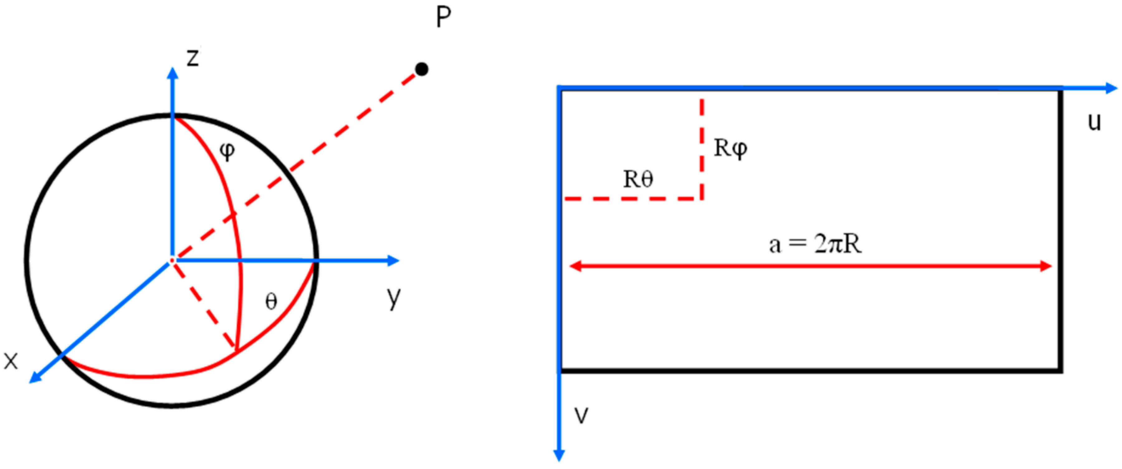
f of the camera. The equirectangular projection is also called latitude–longitude mapping for the relationship between pixel coordinates and geographic coordinates. The sphere is mapped onto a plane using the relationships [
u,
v]
T = R [
,
]
T, where (
,
) are the horizontal and vertical angular directions (longitude and latitude respectively), and (
u,
v) are pixel coordinates (
Figure 2) [
15].
Equirectangular projections are neither conform, nor equidistant or equivalent, so the real angles, distances, and areas cannot be measured using such cartographic representations. The poles of the sphere are converted into two segments with a length equal to the circumference of the sphere. Therefore, the equator and poles have the same length, resulting in strong deformations for zenith and nadir.
The height of the panorama is equal to the length of a meridian. The radius of the sphere is calculated as R = a/2π, where a is the pixel width of the panorama.
Let us suppose that the aim of the problem is the measurement of an area affected by specific deteriorations. Moreover, we assume that deterioration affects a flat wall. After the acquisition of a spherical image, a synthetic rotation along the vertical direction can be applied to change the visualization so that the central point of the wall has longitude θ = 0. First, the equirectangular projection can be synthetically rotated by θ*, so that the new x axis (θ = 0) will cross the median point of the wall.
The synthetic rotation allows for the projection of the point of the sphere onto the plane x = f = R with the simple relationship [1, R tan θ, R (cos θ)−1 cot φ)]T, which encapsulates alignment between the center of the sphere, the point on the sphere, and the point projected on the plane tangent to the sphere in the point [1,0,0]. Here, (R tan θ) and (R (cos θ)−1 cot φ) can be intended as the image coordinates of a new image, which is no longer an equirectangular projection. The new image will be a central perspective (also called pinhole image or frame image). Moreover, the center of the spherical image is also the projection center of the new image.
Obviously, this procedure cannot work with large longitude variations. However, a solution is partitioning the spherical image into four zones kπ/2 ≤ θ < (k + 1) π/2, where the parameter k has the following values k = 0, …, 3. Then, four local pinhole images are derived.
There are several other possible subdivisions of the original image that will produce a larger or smaller field of view. The viewing angle can also be varied to reduce or enlarge the field-of-view (FoV), which may be different than π/2. The case of the ceiling requires to project the images along the Z axis.
2.2. Image Rectification Procedure
A planar projective transformation (or homography) is an invertible mapping from a point in P2 to a point in P2. The transformation is represented by a 3 × 3 non-singular matrix H with 8 degrees of freedom. This kind of mapping is frequently used in photogrammetry and computer vision (CV). Digital rectification is a widely used surveying technique when there are cases of planar objects, as it allows for the direct measurement of metric quantities (angles, distance ratios, and so on). The rectification process can be applied to the original image, which is geometrically modified and resampled in order to make the new image plane parallel to the object. The interpolation of the RGB values can be carried out with different procedures, foe example, nearest neighbor or bilinear/bicubic interpolations. Finally, if several images are employed to cover the entire object, they can be combined to produce a mosaic.
The rectified image gives the opportunity to obtain metric data while preserving the photorealistic effect. For this reason, this methodology is very popular for the survey of objects that can be approximated with a plane (e.g., paintings or building facades, if there are no elements far off the world plane adopted). There exist different commercial softwares capable of performing this task (Perspective Rectifier, PhoToPlan, TriDmetriX, and so on).
It is well-known that a point in the plane is identified as a column vector x = (x, y)T. This pair of values is termed inhomogeneous coordinates. The homogenous coordinates of a point can be obtained by adding an extra coordinate to the pair. This new last coordinate gives a new triplet x = (λx, λy, λ)T, and we say that this three-vector is the same point in the homogeneous coordinates (for any non-zero value λ). An arbitrary homogeneous vector x = (x1, x2, x3)T represents the point x = (x1/x3, x2/x3)T in R2.
A planar homography is an invertible mapping represented by a 3 × 3 matrix:
where
H is a non-singular matrix and has 8 degrees of freedom.
The estimation of
H needs a set of point to point
x′
↔ x correspondences (at least four). The solution with inhomogeneous coordinates is based on the following equations:
where the last element of
H was set to
h9 = 1 to take into consideration the scale ambiguity. Each point gives two linear equations in the elements of
H that are used to write a system of equations of the form
Ah =
b, where
h = [
h1, …,
h8]
T. If four corresponding points are given, matrix
A has eight rows and
b is an eight-vector. This system can be solved for
h using the techniques for solving linear equations (given det(
A) ≠ 0). If more than four point correspondences are given (over-determined set of equations), the solution is not exact and least squares estimation is usually employed.
It is important to say that a camera should be photogrammetrically calibrated beforehand because image distortion generates a misalignment between (i) the perspective center, (ii) the image, and (iii) object points [
7]. It is quite simple to understand that the collinearity principle is no longer respected. Modeling lens distortion allows one to strongly reduce this effect.
Standard photogrammetric projects are often based on images taken with calibrated cameras, where an eight-term (sometimes 10-term) correction model is used to remove the distortion from the image (or from the measured image coordinates
x,
y), starting from the following correction values:
where (
x0,
y0) are principal point coordinates, (
k1,
k2,
k3) are coefficients of radial distortion, (
p1,
p2) are coefficients of decentring distortion, and
r = [(
x −
x0) + (
y −
y0)]
1/2 is the radial distance.
2.3. Rectification of Images Derived from the Equirectangular Projection
Let us consider one of the images obtained from the equirectangular projection. The interior orientation parameters are encapsulated into a calibration matrix:
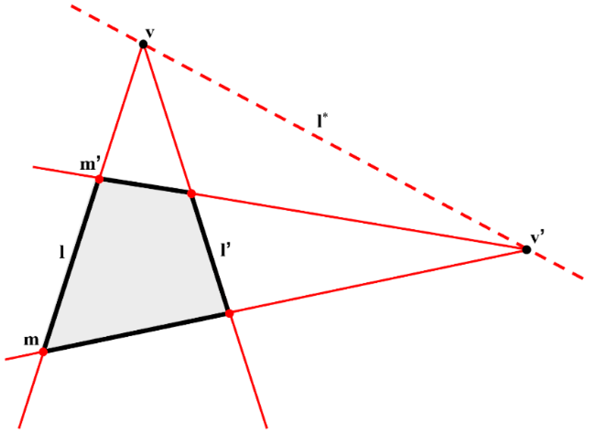
The image has no distortion induced by lenses (e.g., typical barrel and pincushion effects). Thus, no correction must be applied to compensate such an effect. The new image is based now on the pinhole camera model and can be rectified with traditional strategies (e.g., using control points). On the other hand, the calibration matrix provides additional information for the rectification process. If two sets of parallels lines (not necessarily horizontal and vertical) can be identified, the vanishing line
l* can be estimated from vanishing points (
Figure 3), which can be calculated using pixel coordinates. The orientation of the object plane with respect to the camera can be calculated through the normal
n to the plane as
n =
KTl* [
16].
The image can be rectified to obtain a front-parallel view through a homography H = KRK−1, where the unary vector un = n/‖n‖ is aligned to the direction Run = [0,0,1]T. The matrix R is made up of a set of vectors that form an orthonormal set: R = [ur, us, un]T. However, the new frontal image has an ambiguity owing to the rotation around the normal n. In a few words, in three dimensions, there is an infinite number of vectors perpendicular to n. This leads to an under-determined system of equations. To obtain the term of orthonormal vectors ur, us, and un, it is sufficient to generate the unary vector ur and us starting from un. There are multiple solutions to this problem, but a convenient choice consists in generating the final rectified image so that one of the sets of parallel lines will be horizontal (or vertical).
Finally, the rectified image(s) can be imported in CAD software, where the areas can be mapped using different hatches. Such operation is manual and requires an operator expert in condition assessment. The next section shows an example.
2.4. Example of Rectification from a 360° Image and Deterioration Mapping
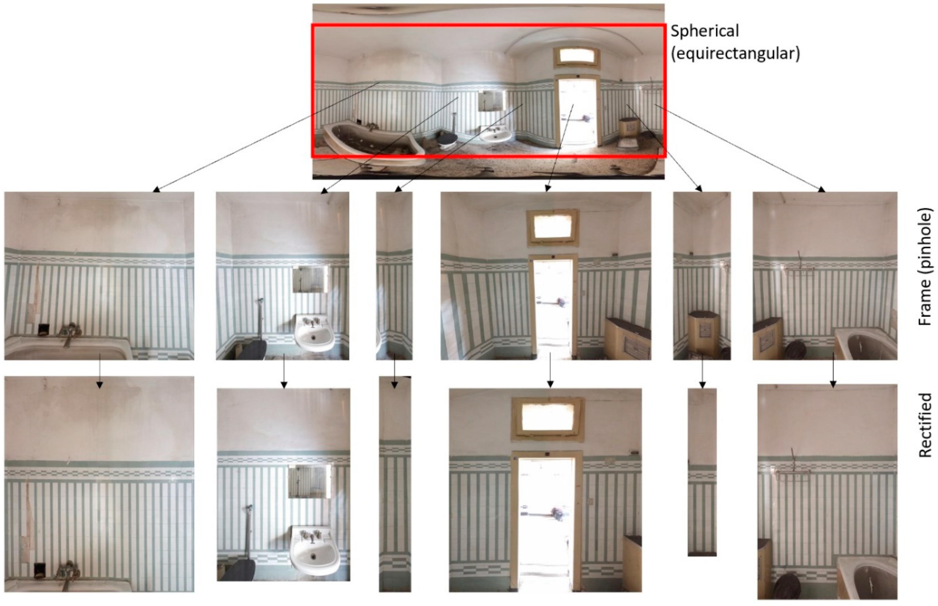
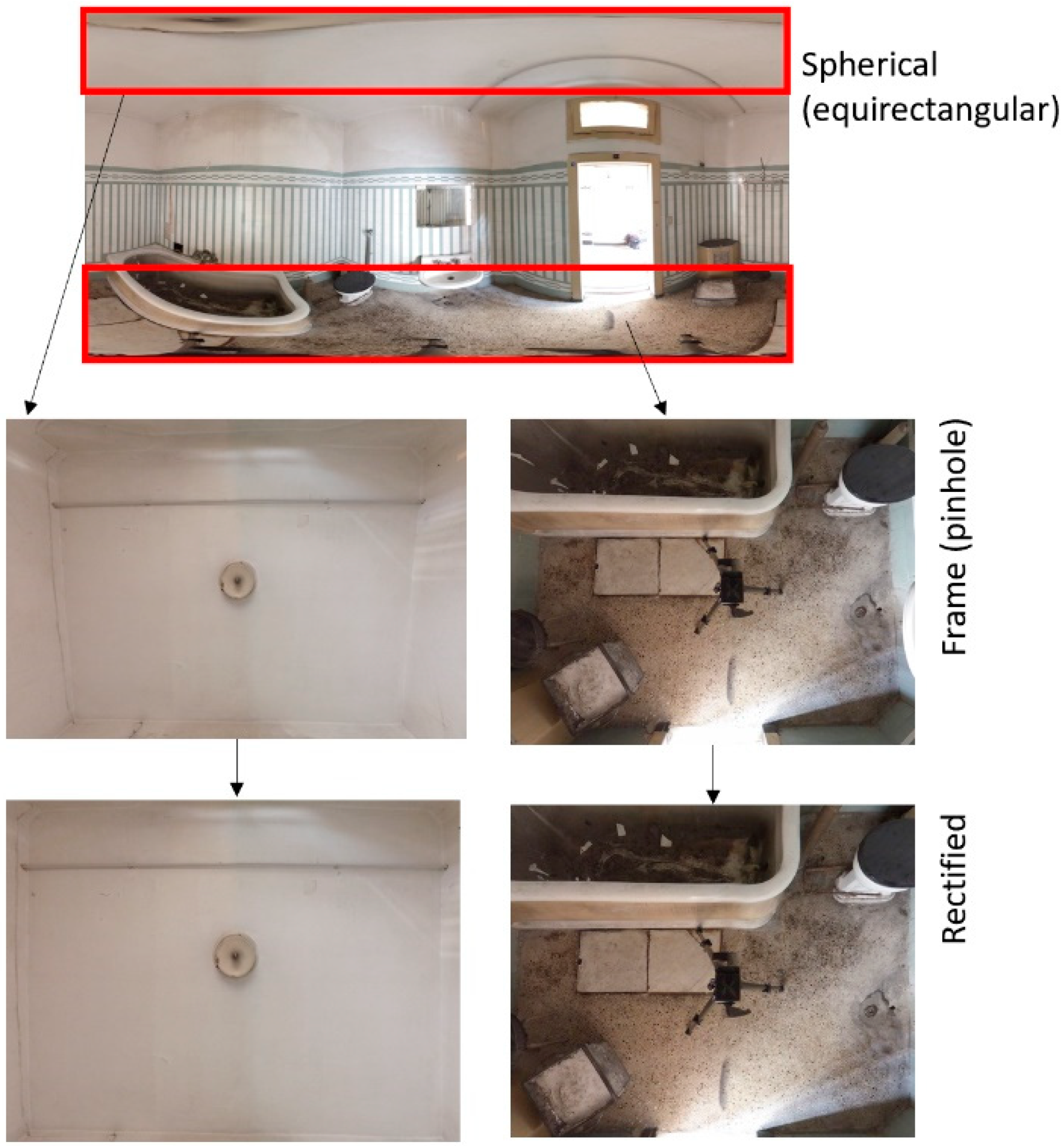
Figure 4 illustrates the overall workflow of the rectification procedure described in the previous section. A single equirectangular image was acquired inside a small room of the Albergo Diurno di Porta Venezia, a hypogea structure located in Milan, Italy. The choice to use a single equirectangular image is motivated by the small size of the room, whose metric documentation with standard rectified photography would require several images for the different walls, and image mosaicking after rectification. A single equirectangular projection is sufficient to capture the whole room, which is then split into the different facades by changing the horizontal angle and setting a sufficient FoV.
The room is not made up of just four orthogonal walls. Small rooms with an angle of 45° are shown in two corners of the room. Such walls cover additional systems, such as the heating plant and the pillars that form the bearing elements of the entire complex. Thus, the equirectangular projection has to be split into six sub-images with a variable FoV, but the same focal length. As mentioned in the previous section, the projection of the point of the sphere onto a local plane tangent to the sphere provides a new frame (pinhole) images, which can be rectified by obtaining metric images.
Obviously, the elements installed on the floor are not rectified, but this is a common issue in all rectification procedures. The expert in conservation is aware of the pros and cons of metric rectification. Overall,
Figure 3 shows the acquired spherical image, the selection of the six new pinhole images, and their metric rectification to obtain measurable images for the following mapping phase.
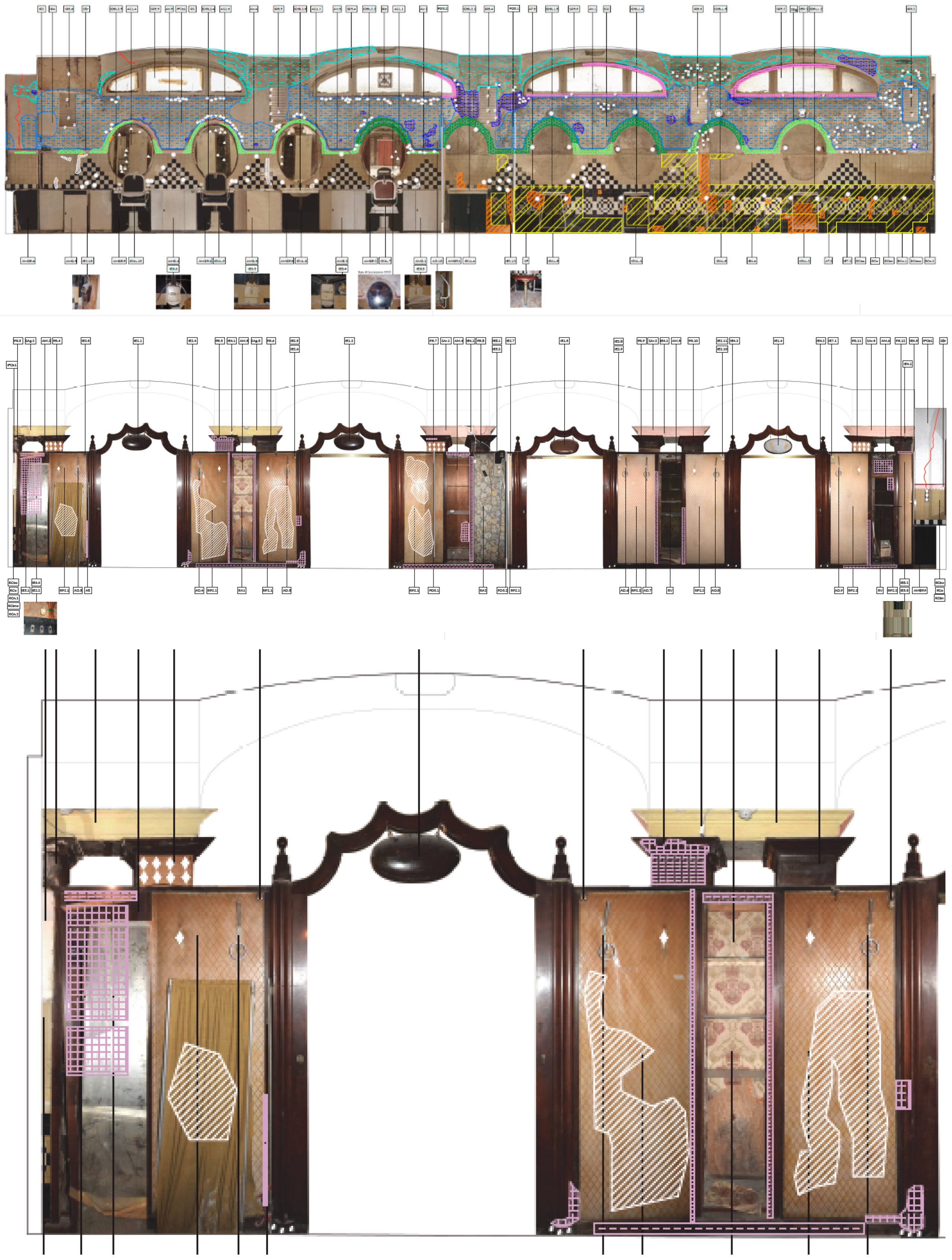
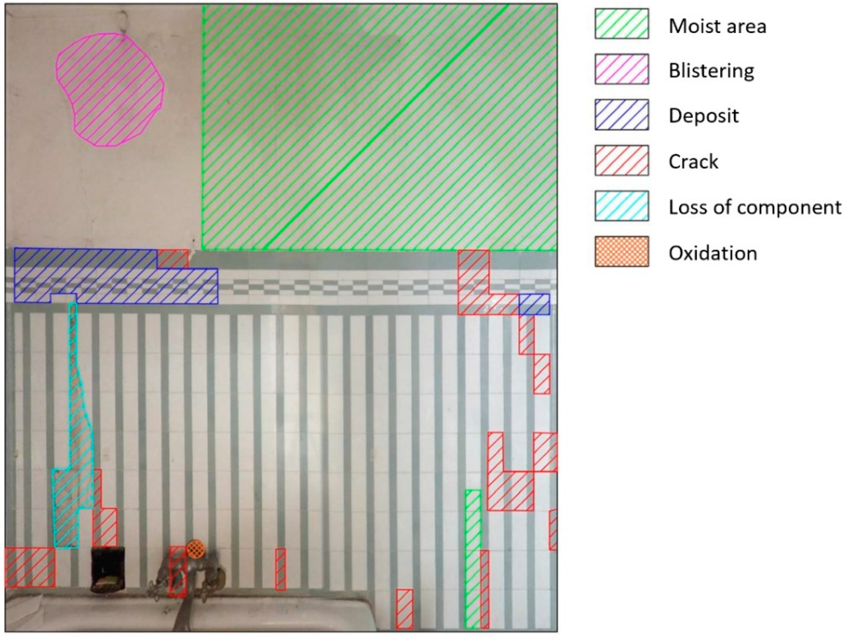
Figure 5 shows one of the facades with the identified deterioration mechanisms. The image was generated with traditional procedures in AutoCAD, applying hatches and measuring their areas. A large moist area reveals a strong deterioration caused by humidity, with a predominant vertical pattern caused by gravity. The effect corresponds to a darkening of the surface. The purple area is affected by blistering, that is, the separation of the outer surface layer that is filled with air. Blue areas reveal a deposit, which is an accumulation of material on the surface caused by the long state of disrepair of the structure. The red pattern identifies those areas with cracks that are mainly located on the tiles. The cyan color indicates the loss of components, that is, the detachment of some tiles probably caused by salts. Finally, the orange pattern shows the elements with an evident oxidation process, resulting in rust on the metal surfaces.
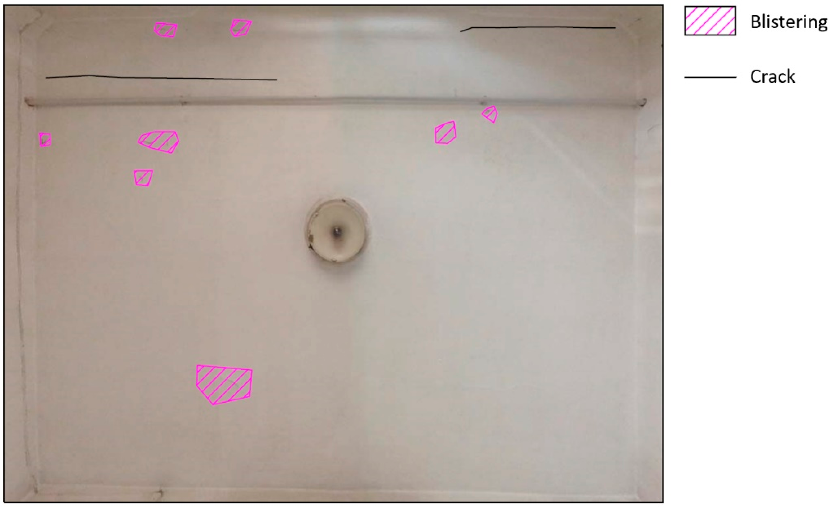
The same procedure may be applied to floors and ceilings (
Figure 6). As the camera was placed in the middle of the room, it is possible to point the visualization of the equirectangular projection to +0° and +180°, setting a sufficient FoV, and then generate the pinhole images. Also, in this case, such images can be rectified using two sets of parallel lines and the value of the focal length.
Figure 7 shows the identified deterioration effects on the ceiling, which are mainly caused by diffused blistering. Some cracks on the plaster are shown as well.
3. Deterioration Mapping Using 3D Modeling with 360° Images
3.1. Three-Dimensional (3D) Photogrammetry with Spherical Images
Most applications of 3D photogrammetry are based on central perspective (also referred to as “frame” or “pinhole”) cameras, notwithstanding, fisheye lenses are also becoming very popular for metric reconstructions for their larger FoV [
17]. It is not the authors’ intention to review here the basic principles of photogrammetry, as several handbooks are available in the technical literature (see, for example, the work of [
18]). The commercial market offers several solutions for automated 3D modeling with a consolidated workflow tie point extraction, bundle adjustment (which may include camera self-calibration if necessary), and dense image matching for surface reconstruction. Examples of software packages for close-range photogrammetry are Agisoft PhotoScan, PhotoModeler, ContextCapture, RealityCapture, Pix4Dmapper, and 3D Flow Zephyr, among others.
This work aims to illustrate that spherical images can be used for 3D photogrammetry, notwithstanding, the geometric camera model used is completely different and requires a specific mathematical formulation. Images (at least two) acquired from different points can be used to create a 3D model. Multiple images can be processed following the typical workflow for image processing based on the spherical (equirectangular) camera model. For some examples of 3D modeling from 360 cameras, the reader is referred to the works in the literature [
19,
20,
21,
22,
23,
24,
25].
Spherical photogrammetry for condition assessment becomes a valid alternative to traditional photogrammetry in the case of elongated and narrow spaces. A small set of spherical images may replace several pinhole images. Moreover, the camera can be oriented to any direction around the vertical axis, because of the 360° data acquisition field that guarantees the complete coverage of the scene all around. This option also simplifies the image acquisition phase when carried out by operators who are not experts in image-based 3D modeling.
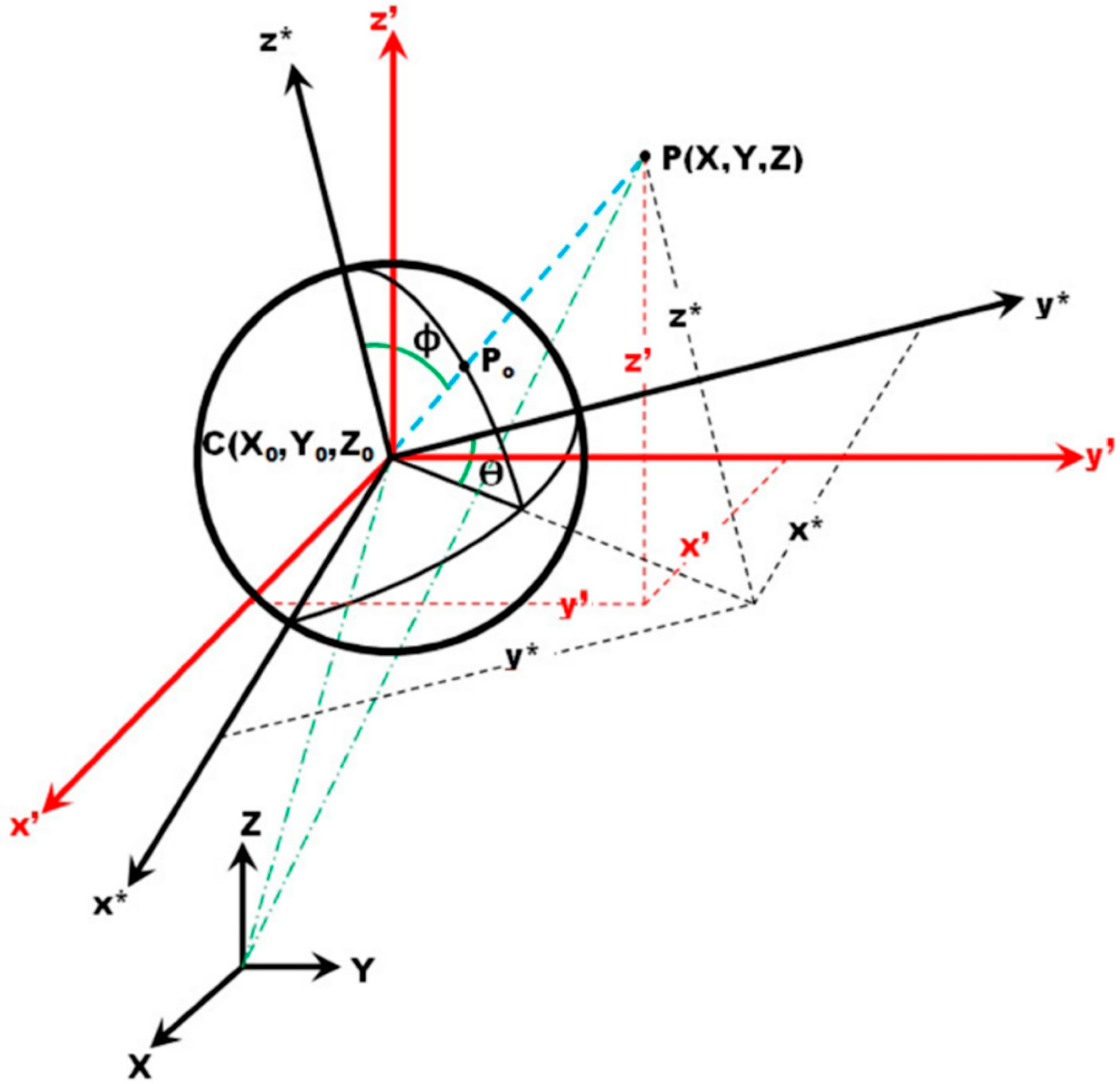
The workflow for spherical photogrammetry is not different from the one adopted with standard pinhole images. What is significantly different is the mathematical model for image orientation, that is, the spherical bundle adjustment that was originally formulated by the authors of [
26], starting from the equations for the adjustment of geodetic networks. As the spherical image can be intended as a unary sphere (pixel coordinates converted into latitude–longitude,
Figure 8), mapping between the image point on the unary sphere
x* = [
x*,
y*,
z*]
T and the corresponding object point
X* = [
X*,
Y*,
Z*]
T is simply expressed by a scale factor λ as
x* = λ
X*. The origin of the (
XYZ)
* reference system is the center of the sphere, while its axes are defined by the convention used for the measurement of latitude and longitude image coordinates. The scale factor is the inverse of the distance between the perspective center of the image (the origin) and the object point. The scale factor may be estimated as
.
A point on a unary sphere has the following coordinates:
where the angles form the observation vector. They are not effective observations, as the operator measures the pixel coordinates (
u,
v). The radius
R of the spherical image is estimated during the stitching of the single pinhole images, and it is the only calibration parameter for these kinds of panoramas.
A single panoramic image can be intended as a data set observed using a theodolite without distance measurement. Indeed, both systems can measure angles along two perpendicular planes. On the other hand, it is not possible to level the spherical image, whereas this operation is quite simple with a total station (thanks to the presence of leveling sensors). This means that an additional correction must be added to correct the lack of verticality, which results in additional parameters to be estimated for the different images. Therefore, the
z* axis associated with the image is not parallel to the
Z axis of the ground system) and two correction angles (
,
) should be estimated and applied around the instrumental axes:
where the rotation matrix
R for not leveled (i.e., the camera is not leveled like a total station) and the panoramic image is as follows:
This method assumes that the angles are relatively small, which is an acceptable assumption in most projects because the set of images is usually acquired without particular tilting of the camera.
The collinearity equations for spherical images may be written with a simple division of the first two rows in Equation (8). In addition, the third row gives the following:
If multiple panoramas are available, they can be adjusted with this new formulation of the camera model, provided that enough corresponding points between all panoramas have been extracted. This results in the fact that, given a set of panoramas and their image correspondences, the poses of the spheres and the object coordinates of the image points can be calculated.
Given a set of panoramas and their image correspondences, the poses of the spheres and the object coordinates of the correspondences can be now determined. The solution is estimated via least squares after their linearization with a Taylor series expansion, beginning from the approximated values for all unknown parameters.
Once the camera (sphere) poses are estimated (with the 3D object coordinates of the image correspondences as well), the reconstruction of the scene can be carried out with normal surveying methods that are based on multiple ray intersections.
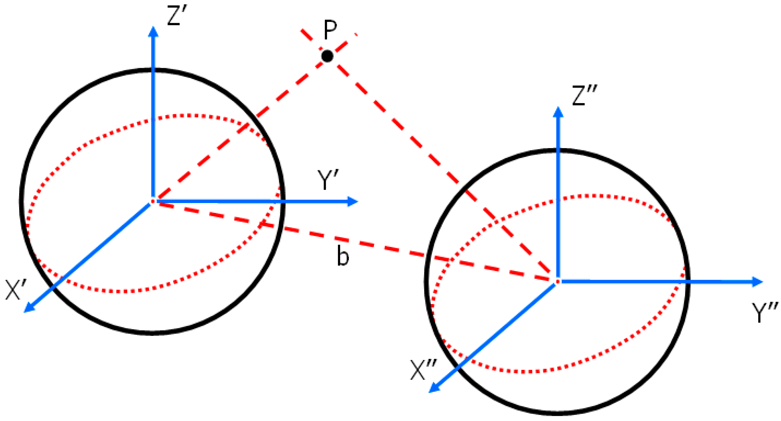
The system can be solved using some 3D control points to remove the datum deficiency and to derive metric results. If no control point information is available, one panorama can be oriented relatively with respect to another one using the coplanarity condition (
Figure 9):
where
bx, by, bz → components of the baseline b between two panoramas;
M′ and M″ → rotation matrices of the panoramas;
X′, Y′, Z′ and X″, Y″, Z″ → object coordinates of two correspondences.
The next sections will illustrate the metric accuracy achievable with such a set of images (
Section 3.2).
Section 3.3 shows how to use a block of spherical images and the product derived from the condition assessment.
3.2. Accuracy Assessment of the Proposed Method
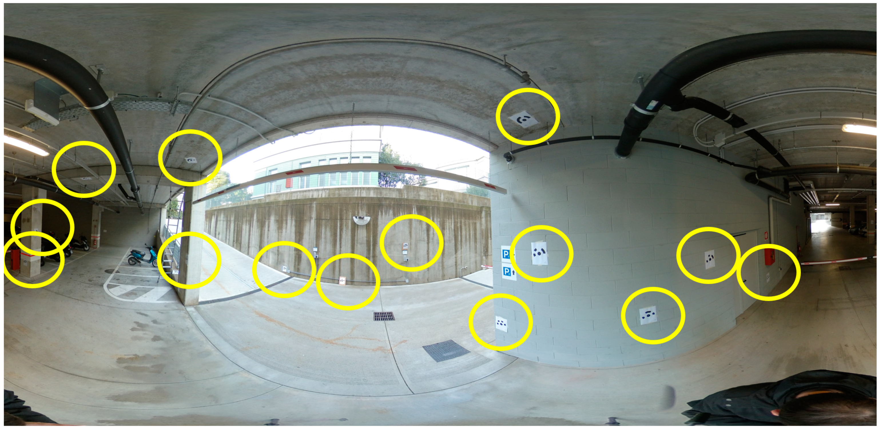
The assessment of accuracy metric of the proposed method was carried out with a set of 15 images acquired with a Xiaomi Mijia Mi Sphere 360. Images were acquired in a garage with bad illumination conditions. In addition, the surfaces have a bad texture and could result in matching issues for the automatic procedures available in the software used. The area has a size of 10.9 m × 6 m × 3.7 m.
A set of targets printed on paper sheets were placed in the area: 6 targets were used as control point and 11 were set as check points. The coordinates were measured with a total station Leica TS30 (angle precision 0.5″, distance precision 0.6 mm), using repeated measurements to improve the metric precision of such a dataset.
Photogrammetric processing was carried out with three solutions: (i) the one proposed in this paper, and the commercial softwares (ii) Agisoft PhotoScan and (iii) Pix4Dmapper. In recent years, some commercial softwares developed considering both photogrammetric and computer vision approaches have added the camera spherical camera model. Examples of software packages supporting this camera model are Agisoft PhotoScan and Pix4Dmapper, for which the traditional workflow used for frame images can be used after setting the spherical camera model. Such software supports the spherical camera model and can be used to process image blocks acquired with the Xiaomi Mijia Mi Sphere 360. The only manual measurement was the identification of target coordinates in the images.
Images were automatically oriented with the tie points extracted by automated matching strategies available in each software. An image of the test field is shown in
Figure 10. Statistics check points are illustrated in
Table 1 and show an accuracy of about 6 mm, whereas the test site is 10.9 m × 6 m × 3.7 m. The relative accuracy achieved is about 1:2000, which is sufficient for metric applications that require the production of deliverables (plans, sections, elevations) at a scale of 1:100.
3.3. Example of Deterioration Mapping using a 3D Model from Spherical Photogrammetry
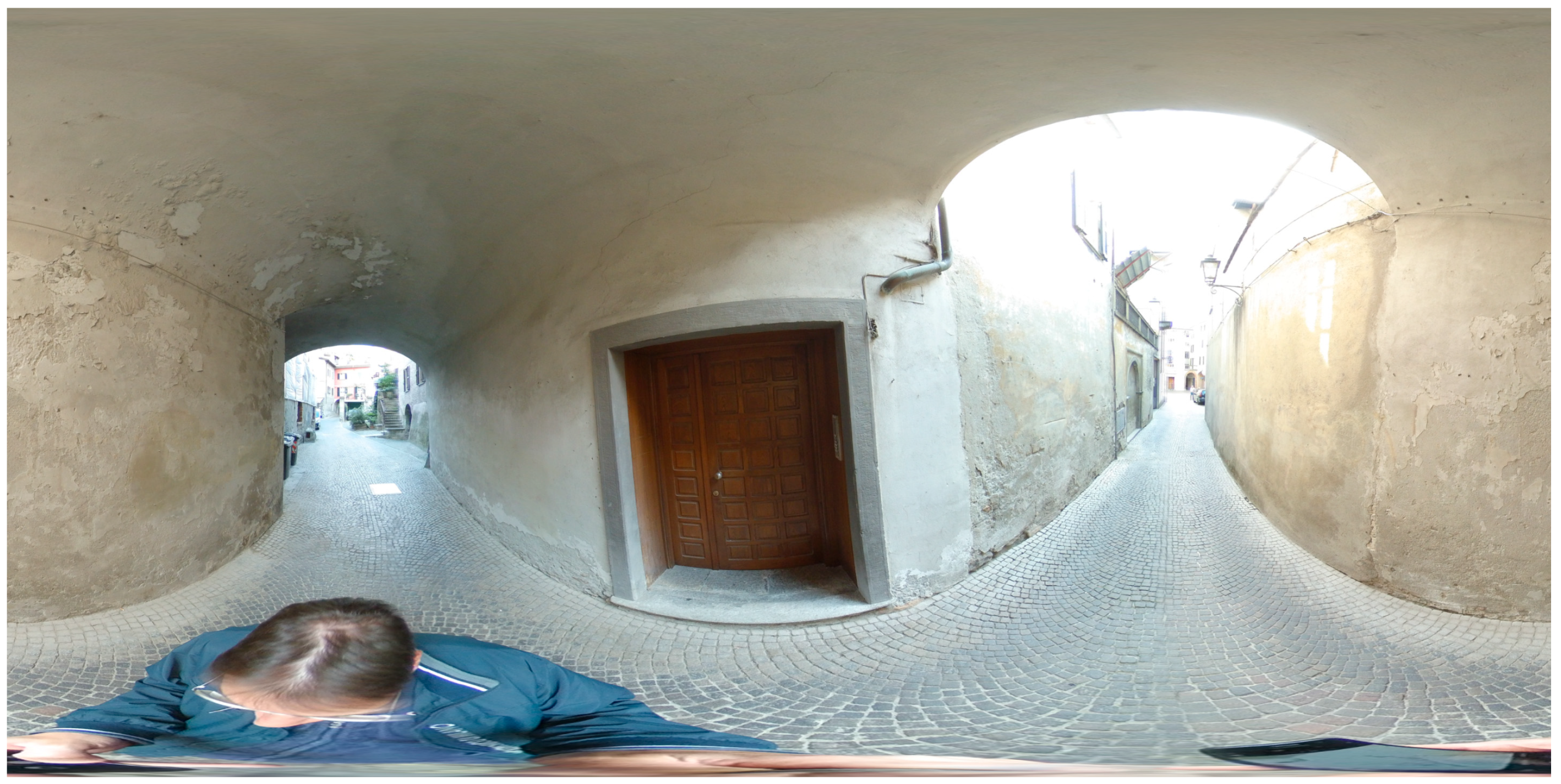
A sequence of eight spherical images was acquired inside a narrow alley, which features two vertical walls and a barrel vault. The camera used in this project is a Xiaomi Mijia Mi Sphere 360, which costs about USD $300. Such spherical images have a (maximum) resolution of 6912 × 3456 pixels and can be created using sets of front- and rear-facing images. The software for image stitching is Madventure 360 Camera, which is available for both mobile and desktop platforms.
Data acquisition was carried out in less than a minute and was a simple operation; that is, the user simply walked along the alley and took the images. The only parameter to be set beforehand was a correct exposure, which ensures a good image quality inside the alley, which is a rather dark space. Acquiring images with good illumination conditions is a fundamental issue in the case of spherical images. As the camera captures the entire scene around the photographer, it is difficult to ensure optimal illumination in any direction. In the case study, images feature good illumination for the vertical walls and the vaults, whereas the area at the beginning and end of the alley is overexposed for the direct sunlight. An example of equirectangular projection is shown in
Figure 11.
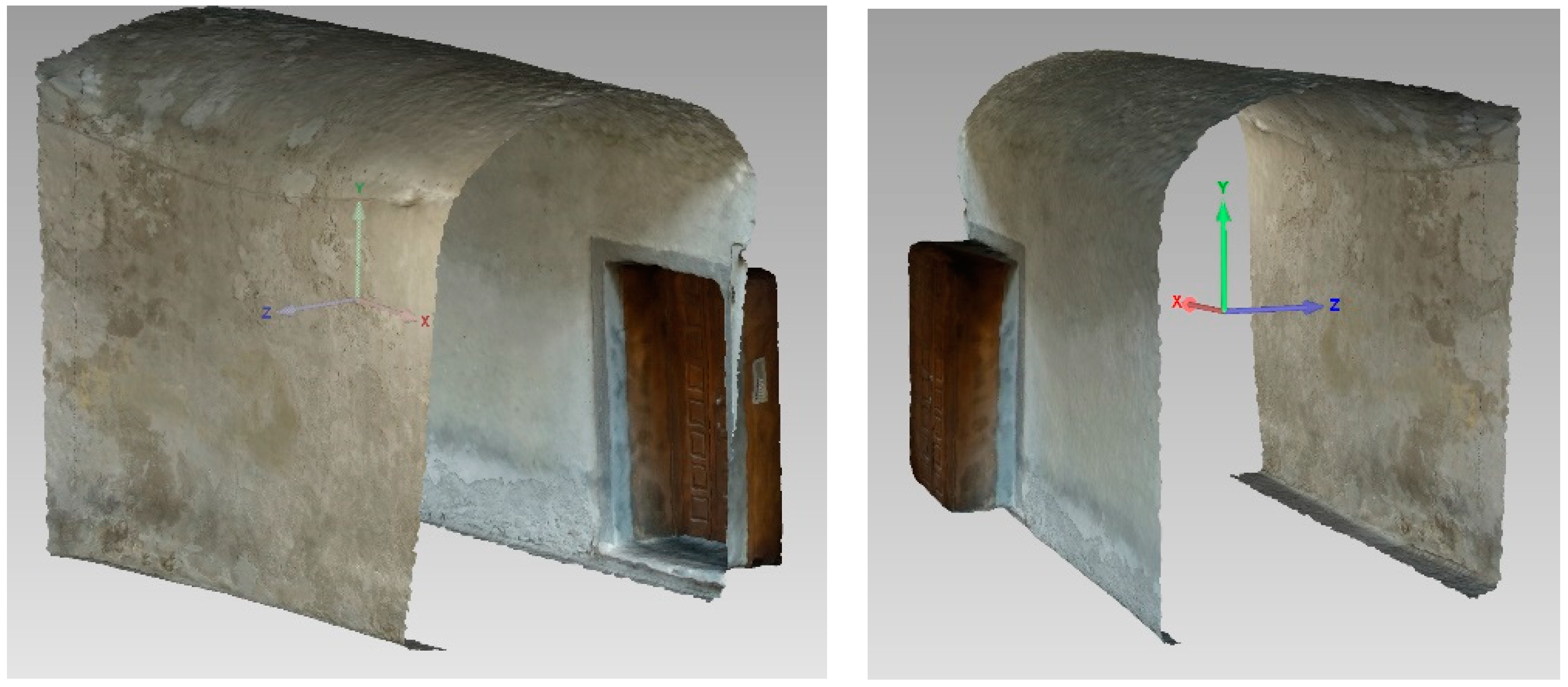
The 3D model generated using the photogrammetric workflow is shown in
Figure 12. As can be seen, a few equirectangular projections can replace many pinhole images required in the standard photogrammetric projects. The model was scaled with a known distance between two points, which was acquired with a tape. Data processing required just a few minutes and resulted in a textured mesh. Such an example demonstrates that a 360° camera can be a valid tool for the survey of narrow spaces, which would require a larger number of images when a traditional frame camera is used.
Finally, digital orthophotos for the vertical walls can be generated, whereas the barrel vault was unrolled to directly measure real areas during the mapping phase.
Figure 13 shows the condition assessment result for one of the walls and the vault. The wall features some cracks at the level of the plaster, which is completely detached in the lower part of the wall because of rising damp, which is a slow upward movement of moisture.
The main problem found on the vault is a diffused exfoliation, which is the detachment of many parts of the superficial layer, which, in some cases, display curling. Some areas affected by moisture are shown as well.
4. Recovering Pixel-to-Pixel Correspondences for Mapping Multi-Temporal Deterioration
4.1. Analytical Details of the Multi-Temporal Registration Procedure
Spherical images can also be used as a rapid tool for inspection and monitoring. The idea is to capture images at different epochs to track changes occurred over time. Such an analysis can be performed at two levels:
In the case when areas need to be computed, it is possible to apply the procedures described in the previous sections to this purpose. An important task in conservation projects is the analysis of changes, which can be identified using a visual assessment. In such a case, it would be useful to generate a multi-temporal dataset of spherical images with perfect pixel-to-pixel correspondence. This result can be simply obtained by placing the camera on a fixed location and then acquiring a set of images at different times. The disadvantage is the need for a fixed camera, which cannot be moved to document multiple rooms.
This section aims to show how to recover pixel-to-pixel correspondence in the case of spherical images acquired at different epochs. The proposed procedure allows the operator to remove the camera, which can be used to document multiple rooms on different projects. The proposed solution is an algorithmic implementation that requires images acquired following specific rules, which are simple also for users who are not experts in image analysis.
Let us start from a simple consideration: spherical images are a kind of panoramic images. It is quite simple to create a spherical panorama without using a 360° camera. Several photos taken from the same point are acquired by rotating the camera around its perspective center. These images are then stitched and mapped with the equirectangular projection.
In this case, the opposite of such a procedure is applied because the 360° camera can directly provide the final equirectangular projection. The idea is to extract a set of frame images (pinhole images) from the equirectangular projection. Such images must feature a sufficient overlap to be remounted with the procedures used for the generation of panoramas.
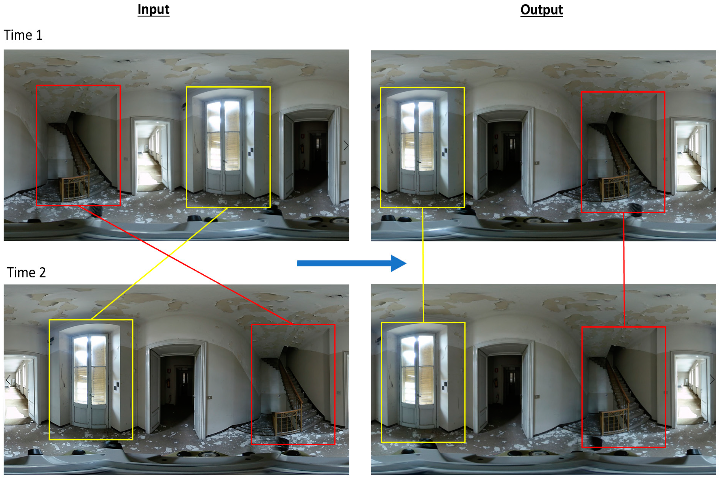
Given the two equirectangular projections and acquired at different epochs from a similar location, the procedure starts with splitting both projections into a set of frame images and , which are processed in a single registration project to regenerate the equirectangular projections and , in which the initial misalignment is compensated for.
If the 360° camera is placed in a similar position during image acquisition at different epochs, we can assume that projections will differ for a repositioning error of the camera. This is because of the different points of view (translation), the variation of the horizontal angle (rotation), and the setup of the camera that is not leveled. The problem becomes similar to the repositioning of a total station on the same point, in which the horizontal circle will be oriented differently, plus the additional issues related to the lack of a leveling sensor in the camera.
As mentioned, both spherical images are split into multiple pinhole images. First, a set of 12 pinhole images is generated from one spherical image. Each image has an FoV of π/2 × π/2; a focal length equal to the radius of the sphere; and the central point of each image corresponds to a longitude Nπ/6, in which N assumes the following values: 0, 1, 2, …, and 11. Then, another set of images is acquired by varying the vertical angle of π/4. This allows us to generate a novel set of eight images with an FoV of π/2 × π/2, acquired every Mπ/4, where parameter M has the values 0, 1, 2, and 3. Finally, one image is acquired using a variation of +π/2 to produce vertical panoramas looking towards the vertical direction.
The reader could ask why a set of images was acquired applying a pitch variation of π/4. The reason is the lack of overlap between the images with just the horizontal angle variation and the two vertical images. In that case, an FoV of the images of π/2 × π/2 does not provide any overlap in the matching phase, so it causes failure in the data processing.
The subdivision procedure generates 21 images that are central perspectives and can be reused to generate the equirectangular projection. The original projections can be recreated using a mathematical formulation based on projective geometry. Indeed, the transformation between two pinhole images acquired by a rotating camera is a homography [
27]:
and
As the aim is to register two equirectangular projections acquired from a similar position, both projections are into a set of frame images. Then, two new equirectangular projections are generated using a bundle adjustment formulation able to compensate for the lack of alignment. The 42 images derived from both projections are used in single adjustments to compensate for the lack of pixel-to-pixel correspondence of the original projections.
Matching is carried out with the scale invariant feature transform (SIFT) operator [
28] in order to extract a set of features from the images. All descriptors are compared with fast algorithms able to reduce the computational cost [
29,
30]. Finally, the matched image points allow the estimation of the unknown parameters with a bundle adjustment based on the Levenberg–Marquardt algorithm [
31]. During the stitching process, the compensation of radial distortion is not applied as the images generated from the equirectangular projection are distortion-free. Enhancement procedures can reduce the radiometric differences between consecutive images. Gain compensation is applied to reduce the intensity difference between overlapping images; then, a multi-blending algorithm removes the remaining image edges, avoiding blurring of high-frequency details.
The procedure can recover the lack of alignment if the camera is replaced on the same point with millimeter-level accuracy. The repositioning on the same point generates a parallax effect between the two set of frame images, which can be intended as a 3D shift of the perspective center of the new frame images. After the estimation of the image parameters in a single adjustment, the new equirectangular projections are generated using a common reference system.
4.2. Experiment with a Sequence of Multi-Temporal Images
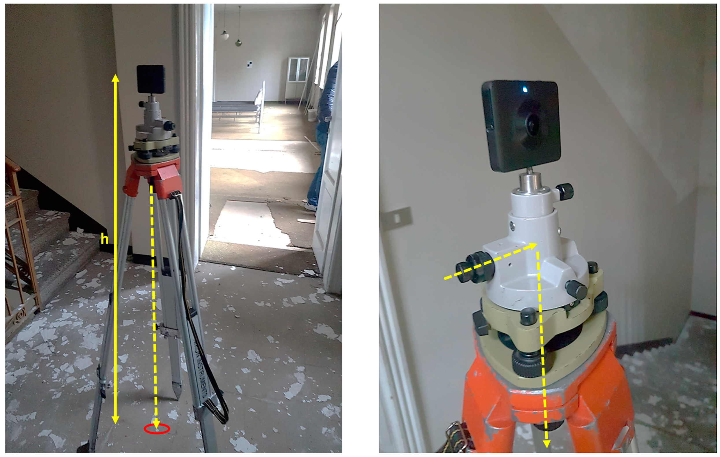
Figure 14 shows the special tool used for accurate repositioning, which is a surveying tripod placed on the same point. The 360° camera is installed on top of the tribrach installed on the tripod, and the center of the projection will be aligned along the vertical direction through a point marked on the ground. The advantage of the optical tribrach is to allow repositioning the camera on the same point. It is also important to measure the instrumental height so that the tripod may be set up at different measurement epochs with an error limited in the order of 2–3 mm.
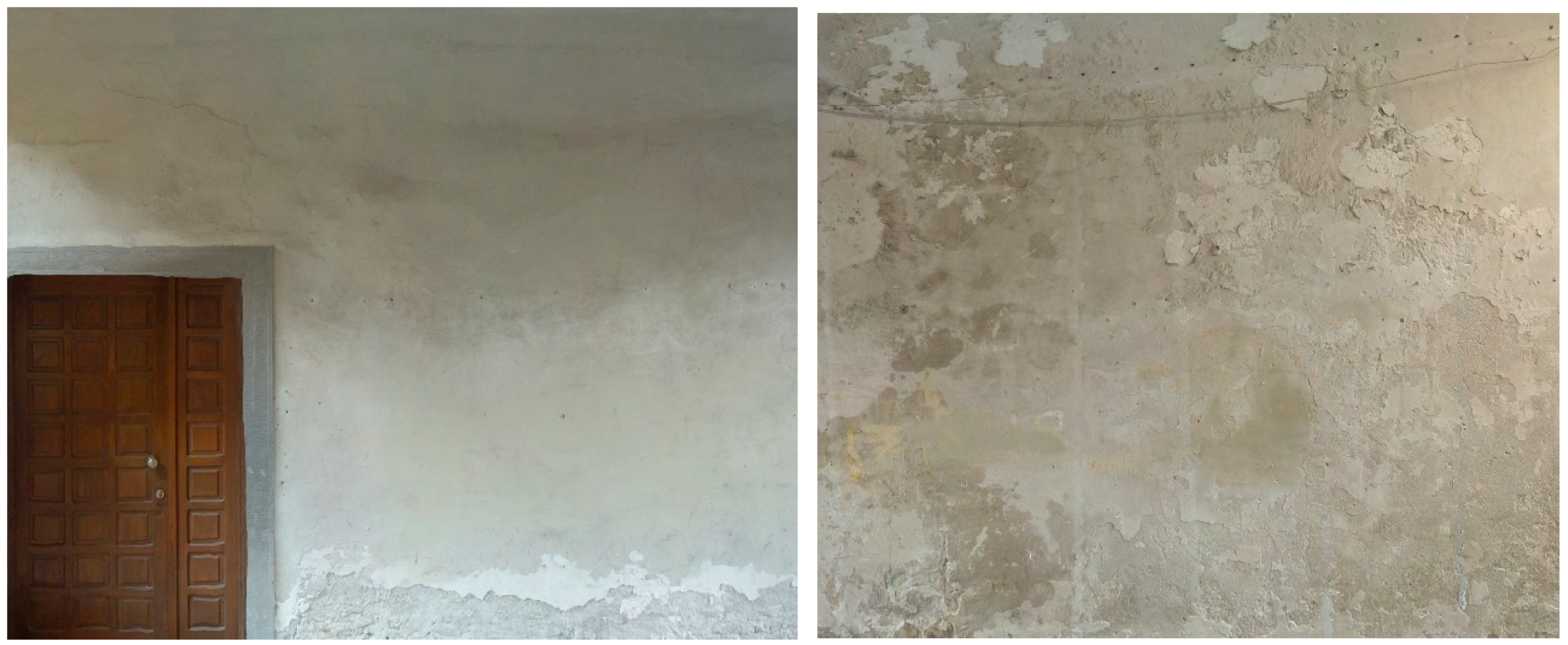
The experiment was carried out in the narrow space along a staircase of a historic building. The building features several deteriorations, which are mainly exfoliations for the considered area.
Two equirectangular projections were acquired at different times, obtaining the images in
Figure 15. Both projections were split into 21 frame images, obtaining the input dataset for the registration procedure based on the bundle adjustment of images acquired with a rotating camera. The use of the repositioning system allows users to get a residual error of ±2–3 mm on the perspective centers. The statistics of least squares adjustment resulted in a misalignment of ±2 pixels, mainly caused by the lack of perfect alignment, as expected. On the other hand, such an error is surely acceptable for visual change detection, for example, the principal operation performed by operators interested in evaluating the changes occurring from a sequence of multi-temporal equirectangular projection.
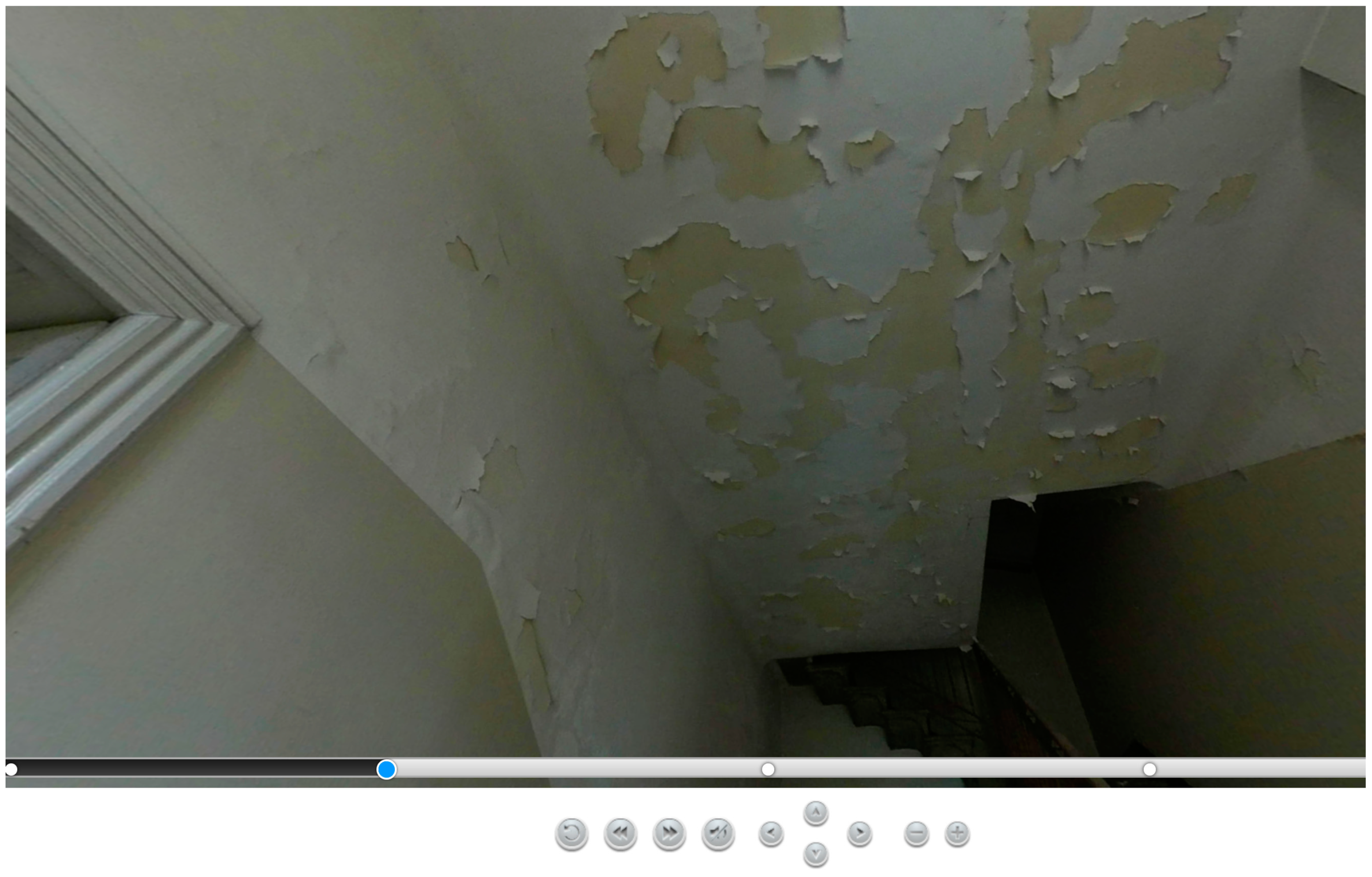
The virtual environment (
Figure 16) is available in HTML format so that it is accessible through a web browser, not only limited to personal computers, but is accessible on mobile devices such as phones and tablets. This means that it can be directly used on-site, offering the opportunity to inspect the structure not only in the office. A sliding bar is also available to allow a smooth transition between different images. Images are placed in different layers so that the user can activate specific images and analyze the changes that occurred. This allows the user to inspect images acquired at different epochs, revealing the occurred changes.
The inspection in the virtual environment has shown the growth of the exfoliation effect, especially for the area on the ceiling. Several detached fragments are also shown on the floor. Minor exfoliation is also shown on the lateral walls. The use of multiple images acquired at different epochs has revealed that deterioration conditions are stable.
The model can also be integrated into virtual reality devices. Indeed, equirectangular projections have a strong relationship with virtual reality [
32]. In this work, the case shown in
Figure 16 was successfully exported and tested in multiple solutions, including Google Cardboard, VR Box, Oculus Rift, and Samsung Gear VR. The opportunity to simulate human vision (notwithstanding that the visualization is limited to a single point at present) is a novel way to execute traditional operations for material, construction technologies, and deterioration assessment. Future work will consist of the extension to multiple locations accessible in the same projects, as well as the implementation of some tools to perform visual assessment in the virtual environment. This will require the integration of mapping operations based on touch controllers, which are already available on the commercial market.
After collecting images with a 360° camera, the creation of the virtual environment is carried out using 3DVista Pro. The software allows one to produce virtual reality tours based on panoramas, which simulate multiple points of view, like in the case of a “static” observer. In fact, virtual navigation is a rotation of the point of view, without the opportunity to freely navigate the scene (translation). Complete navigation is instead possible when a complete 3D model is available.
A sliding bar allows the user to move the visualization between the original image, the image with additional information about construction technologies, or the image with information about condition assessment and pathology descriptions. The selection of specific elements provides extra windows, revealing other files that can be downloaded, printed, or used directly in the virtual tour.
The method is also able to incorporate additional information in terms of new spherical images (e.g., those acquired in different periods for the analysis of the occurred changes), or information in terms of descriptions, external photographs, videos, new drawings, charts, weblinks, and so on.
5. Conclusions
The paper described some examples and applications of condition mapping with 360° images. These kinds of images have been unexplored in the field of restoration and preservation of historic construction. Also, the lack of commercial software able to carry out some of the tasks described in the paper required the implementation of novel procedures for turning 360° images into metric products.
The measurement of accurate areas from 360° images is a promising solution for small and narrow spaces in which the restoration project would require many traditional frame images. A single 360° projection can be split and processed to generate a set of rectified images from which deterioration areas can be identified and measured. In the case of irregular architectural elements featuring a 3D geometry, spherical images can be processed to generate accurate 3D models with a bundle adjustment formulation based on the spherical camera model. Then, digital orthophotos provide the project deliverables for deterioration mapping.
Finally, a novel method for visual assessment based on a set of multi-temporal spherical images was presented and discussed. Such images can capture the entire scene around the camera and are an efficient and rapid mapping tool for both visual and metric assessment.
The growing availability of low-cost 360° cameras requires new algorithms able to efficiently provide metric information, beyond traditional visualization purposes. Spherical photogrammetry combined with new efficient visualization methods can have an important role in a variety of real applications, including the case of material and condition assessment presented in this paper.
Future work consists of the development of algorithms able to assist with automated change detection. After the registration of a set of equirectangular projections, the procedures developed in the field of remote sensing can be used to reveal the changes that occurred. Research work is still required for reliable identification of changes, as well as for those parts in the images that are very distorted in equirectangular projections (e.g., floors and ceilings).


