Transport System Models and Big Data: Zoning and Graph Building with Traditional Surveys, FCD and GIS

Abstract

The paper deals with the integration of data provided from traditional transport surveys (small data) with big data, provided from Information and Communication Technology (ICT), in building Transport System Models (TSMs). Big data are used to observe historical mobility patterns and transport facilities and services, but they are not able to assess ex-ante effects of planned interventions and policies. To overcome these limitations, TSMs can be specified, calibrated and validated with small data, but they are expensive to obtain. The paper proposes a procedure to increase the benefits of TSMs’ building in forecasting capabilities, on one side; and limiting the costs connected to traditional surveys thanks to the availability of big data, on the other side. Small data (e.g., census data) are enriched with Floating Car Data (FCD). At the current stage, the procedure focuses on two specific elements of TSMs: zoning and graph building. These processes are both executed considering the estimated values of an intensity function of FCDs, consistently with traditional methods based on small data. The data-fusion of small and big data, operated with a Geographic Information System (GIS) tool, in a real extra-urban context is presented in order to validate the proposed procedure.

1. Introduction

The decisions that modify the transport system require the support of an ex-ante quantitative analysis. The performances of the current transport system must be evaluated through indicators to determine if any, and which, interventions and policies are necessary. Therefore, it is necessary to obtain measures of levels of sustainability (social, environmental and economic).

In this regard, Information and Communication Technologies (ICTs) have been available in recent years to monitor the components of the transport system (transport facilities and services, people and freight mobility, and vehicles). For what concerns mobility, monitoring systems are composed of sensors and data acquisition tools able to provide historical and/or real-time traffic measures.

In a planning context, it is necessary to define a future configuration of the transport system able to overcome critical issues by ensuring the current and future mobility needs in a sustainable way. In order to ensure this, it is necessary to build Transport System Models (TSMs) that represent each single component of the transport system and the mutual interactions. Inference statistics from big data are not valid in every context, especially if planned transport configurations are far from the current one.

TSMs allow the analysts and planners to determine the critical elements and, therefore, to obtain ex-ante estimates of planned transport system configurations (e.g., new transport infrastructures or changes of existing services). The construction of TSMs requires the collection of data that can be expensive, if it is done with traditional methods. In particular, surveys are necessary on all the components of the system and on the mutual interactions, whose results are essential in the phase of parameters calibration.

In this paper, the authors refer to traditional and consolidated TSMs based on a network approach. This approach requires as first step the zoning and graph building. The accuracy of this representation is decisive for TSMs building. The use of traditional approaches integrated with big data increases the quality of the models. The data collection necessary for the phase of parameter calibration is burdensome, especially by using traditional methods.

The recent development and widespread diffusion of ICT tools, such as mobile phones, allows to observing large sample sizes and long observation periods concerning people and freight mobility (big data for mobility). However, if the transport system changes, for example as a result of choices made by transport operators, the big data analytics approach has limitations. In fact, without the support of TSMs, they do not allow to forecast the effects connected to transport system scenarios.

One the modelling side, despite the availability of the several big data sources, TSMs commonly used in planning activity are supported, almost exclusively, by traditional data such as travel surveys, population census, traffic measures.

The paper attempts to ask to the general research questions concerning the definition of the mutual interactions between ICT and TSMs, in order to integrate them into an Intelligent Transport System (ITS) [1,2], where each component plays the most appropriate role.

The contribution of the paper regards the integration between TSMs and big data in order to maximize the individual benefits and increase the capacity of transport analysts and planners to analyze, forecast, and plan mobility phenomena. Traditional methods to build TSMs are enriched with big data for mobility. In this regard, the authors propose a procedure that follows the steps adopted by traditional methods of transport systems engineering [3]. The typical activities carried out in each step are supported by the use of big data for mobility. The procedure was built with particular reference to road transport systems, focusing on graph buildings regarding transport supply, and zoning, for what concerns travel demand.

The proposed procedure contributes to increase model accuracy and to reduce costs generally imposed to build TSMs implementing traditional approaches with expensive surveys. Integration of information deriving from ICT (e.g., Floating Car Data, FCD) inside a transport modeling framework requires lower quantity of financial resources, due to their availability in the market.

After this introduction, the paper is organized as follow. Section 2 reports a literature review on TSMs and relative methods, and on big data applications for mobility. Section 3 presents the procedure that allows planners to benefit of the potentialities of big data to build two important components of the TSMs, which are zoning and graph building. Section 4 illustrates principal results of an experimentation aimed on validating the procedure in an extra-urban area in the South of Italy. The last section reports the preliminary conclusions and the research perspectives.

2. State of the Art

The section is articulated into three parts. The first presents a state-of-the-art of two components of the so-called TSMs, which are transport supply and travel demand. The second reports a state-of-the-art concerning the applications of big data to estimate the two above modelling components of TSMs. The third presents the research contribution of the paper, starting from the gaps emerged from the state-of-the-art.

2.1. Transport System Models

TSMs allows transport analysts and planners to simulate and design the transport system. TSMs have been developed according to two different approaches [4]: design approach, and scenario-simulation approach. As far as concern the former, TSMs find an optimal configuration (scenario) of the transport network, according to a set of performances and impacts criteria (e.g., total delay, energy, emissions minimization). As far as concern the latter, TSMs simulate and estimate transport system performances and impacts (e.g., total delay, energy, emissions), given a configuration (scenario) of the transport network.

Transport supply. Transport supply models simulate performances and traffic flows, resulting from users and from transport infrastructures and services [5,6,7,8]. In the most common developed approach, transport supply models are represented by a network model (with links and nodes), where a graph can be primary versus dual and cost functions can be aggregate (e.g., speed-density or time-flow relationships) or disaggregate (e.g., car-following, lane-changing, gap-acceptance models). By considering the aggregate case, if the link cost is supposed to be dependent on traffic flow, at least in one link, the network is defined as congested; if not, the network is not-congested.

Travel demand. Travel demand models simulate users’ choices resulting from activities and infrastructure and service performances [3,5,9,10]. Travel demand models can be not-behavioral or behavioral. The latter can be gravitational-entropic or regressive, while the former can be based on random utility, fuzzy or quantum utility theories. Travel demand models simulate the travel purpose, the departure time, origin, destination and mode, route of users.

2.2. Big Data for Mobility

The paragraph reports a state-of-the-art concerning the applications of big data to estimate modelling components of TSMs, in particular the transport network (based on graph building) and travel demand, starting from travel behavior for obtaining origin–destination (OD) flow matrices (based on zoning).

Big data obtained from the numerous ICT tools are a precious source of information about transportation system. Sensors may be classified into two classes. In-vehicle sensors (i.e., GPS on-board, mobile phones) [11,12] allow to obtain space-time coordinates of vehicles along the road network (i.e., FCD). Out-vehicle sensors can be classified into tripwire, able to operate on a road section measuring vehicular flows, speeds, and other variables; and tracking, able to operate on an extended road area and to track vehicle trajectories [13,14].

There is a promising research line dealing with the integration of traditional travel diary surveys, census and traffic counts data, with big data generated from different available big data sources [14,15,16]. The great challenge for transport modelers and planners is to find solutions that are capable to filter, integrate and convert big data obtained from ICT sensors into estimates of travel demand and infrastructure performances. These applications analyze historical and real-time data aimed at providing information to decision-makers and to travelers about the current conditions of the transport system.

Among the existing literature, the authors selected some papers that present procedures and case studies concerning the use of big data, sometimes in synergy with data collected from traditional surveys, for build modelling components of TSMs.

Several papers deal with the use of big data (i.e., FCD, or Call Detail Records, CDR) to estimate passengers’ travel behavior or OD flow matrices. Wang et al. [17] investigated driving behavior through FCD collected close to the University of Michigan (USA). They combined FCD with geocoded street addresses, land-use polygons, aerial photographs, census data, and road attributes. Ribeiro et al. [18] evaluated the influence of different sources of travel information—FCD recorded compared to self-reported—in travel demand models. According to them, FCD technology collects the travel patterns more precisely reducing the bias by collecting data from short trips not reported in traditional surveys. Chen et al. [19] stimulated the debate between travel behavior researchers, who have long relied on household travel surveys (small data), and big data researchers, who use passively-generated data (big data). Lwin et al. [20] used one-week mobile CDR and a Geographic Information System (GIS) road network model to estimate hourly link population and flow directions, based on mobile-call activities of origin–destination (OD)-pairs with a shortest-path analysis for the whole city. Wismans et al. [21] used mobile phone data (CDR) for enriching the transport model of the region of Rotterdam. The raw data are processed into basic information, which is subsequently translated into OD-information, based on several decision rules. Toole et al. [22] estimated multiple aspects of travel demand using CDRs from mobile phones in conjunction with open- and crowdsourced geospatial data, census records, and surveys.

Few are the papers that use big data to estimate network and infrastructure performances (i.e., travel costs). Guo et al. [23] proposed an approach that treats vehicles trajectories as a complex network and uses spatially constrained graph partitioning methods to find spatial structures and general patterns in trajectories. Toole et al. [22] present a solution to build an optimized road network by means of a “Boost Graph Library”, which is a flexible and efficient tool, and to estimate congestion (volume-over-capacity), and travel times for all road segments. Oloo F. [24] tracked motorcycle taxis in a rural area in Kenya, by tagging volunteer riders with GPS, and applied a semi-automatic procedure on the resulting trajectories to map rural-level road networks. The results showed that GPS trajectories could potentially improve the maps of rural roads and augment other mapping initiatives (i.e., OpenStreetMap).

2.3. Existing Literature Gaps and Research Contribution

Pro and cons of TSMs. TSMs support transport modelers and planners in assessing the effects of planned scenario concerning the transport supply (i.e., transport infrastructure and services) and the passenger and freight mobility. The model building protocol (specification, calibration and validation) of TSMs for the current conditions and planned scenarios of transport systems allows to estimate the travel demand, which is composed of transport users, the transport costs or disutilities, connected to trips [3,5]. It allows evaluating the a-priori effects and the costs and benefits of the forecasted scenarios. While TSMs have become more sophisticated and progressively evolved from trip- to activity-based during the last years, the above model building protocol is still based, essentially, on travel diary surveys covering a small sample of the population (small data). The data collection necessary for the parameter calibration phase is burdensome.

Pro and cons of big data for mobility. Big data concern observations of large sample of population and long observation periods concerning people and freight mobility, in contrast of the small data obtained with traditional surveys. The problem connected to big data is that they are sparse and noisy; therefore, a great effort is necessary to filter, integrate and convert them into estimates of travel demand and infrastructure performances. It is worth noting that big data refer to historical, or at most real-time, conditions of the transport system and they do not provide any insight about its future. Only regressive estimations are allowed for scenarios similar to the observed one. For new scenarios, different from the current one, forecasts from historical data are not statistically correct.

Research contribution. The literature left out some areas where the integration between big and small data could be beneficial in building (parts of) TSMs. This is a win–win game for both TSMs and big data analytics approaches. One area is the determination of zones within a study area, called zoning. While transportation researchers have long used traffic zones, that big data analysts have often relied upon uniform grids or lattices. The paper tries to answer to the question such as what method can be applied to identify a zone using available big data (i.e., FCD) that is consistent with traditional methods based on small data on mobility patterns. Another area concerns the (road) graph building. The traditional methods of transportation researchers take into account the types of road elements classified by road width (e.g., motorways, highways, local). The contribution of big data could concern the identification of the types of roads, according to the estimated values of an intensity function of FCDs inside an area (of a given radius) or along a link.

3. An Integrated Procedure

The proposed procedure integrates traditional transport methods and models and big data. In particular, FCD are used with other information in order to build TSMs developed for simulating road transport system. In this paper, the zoning and graph building elements are considered.

3.1. Definitions and Notations

This paragraph reports the definitions and notations that are used in the description of the proposed procedure.

A detected position of a (road) vehicle, P(x, y, t), is defined as the knowledge of its spatial (x, y) and temporal (t) coordinates, in relation to a geographical area.

The influence area of P is defined as the portion of a geographical area where the influence of P is greater than zero. The influence area is limited by an influence area boundary.

A decay function of the influence of P is defined as function that has its maximum value in correspondence of P, null value outside the influence area, and it is monotonically decreasing from P to the influence area boundary. The “distance” between P and each point of the area boundary is denoted with r_max. The influence of P could depend on different measures of “distance”: Euclidean distance, road distance, disutility, etc.

Given a geographical point of the study area, the intensity function is obtained as the sum of the values of all the decay functions of the influence of P in the point.

The study area defines a geographical area, which includes the examined transportation system and most of the effects generated in the forecasted scenarios. The study area is limited by a study area cordon or boundary. The area outside this boundary is called external area, which is considered for its connections with the study area (i.e., commuting trips).

Trips undertaken in a given area may start and end in any geographical point (the space is continuous). In order to let the transportation system be modelled, the study area (and parts of external area) must be discretized into a finite number of traffic zones. Trips between two different zones are defined as inter-zonal trips, while trips starting and ending within the same traffic zone are defined as intra-zonal trips.

A graph, used for modelling transportation supply, G = (N, L) is defined as an ordered pair of sets: N is the set of elements called nodes, and L ⊆ N × N is a set of pairs of nodes belonging to N, called links.

Links represent phases and/or activities of (passenger and freight) trips between different traffic zones. They can represent an activity connected to a physical movement, or not. Links identify segments of trips of equivalent characteristics; in a road graph, drivers travel at the same average speed in a road section with homogeneous physical and functional characteristics.

Nodes are associated to relevant elements/events identifying the segments of trips (links). They can correspond to points with different space and/or time coordinates, where the events occur. In a road graph, nodes are typically associated to road intersections.

Centroids are ideal points where the beginning and/or the end of individual trips related to a traffic zone are concentrated [3].

Zoning is typically operated by identifying portions of the study area, which present homogeneous characteristics in terms of geography, physics, topology and transport [3].

Graph building consists in the topology representation of road infrastructures and services (topological supply component) and in the connection of G with centroids (topological demand component).

3.2. Transport System Models

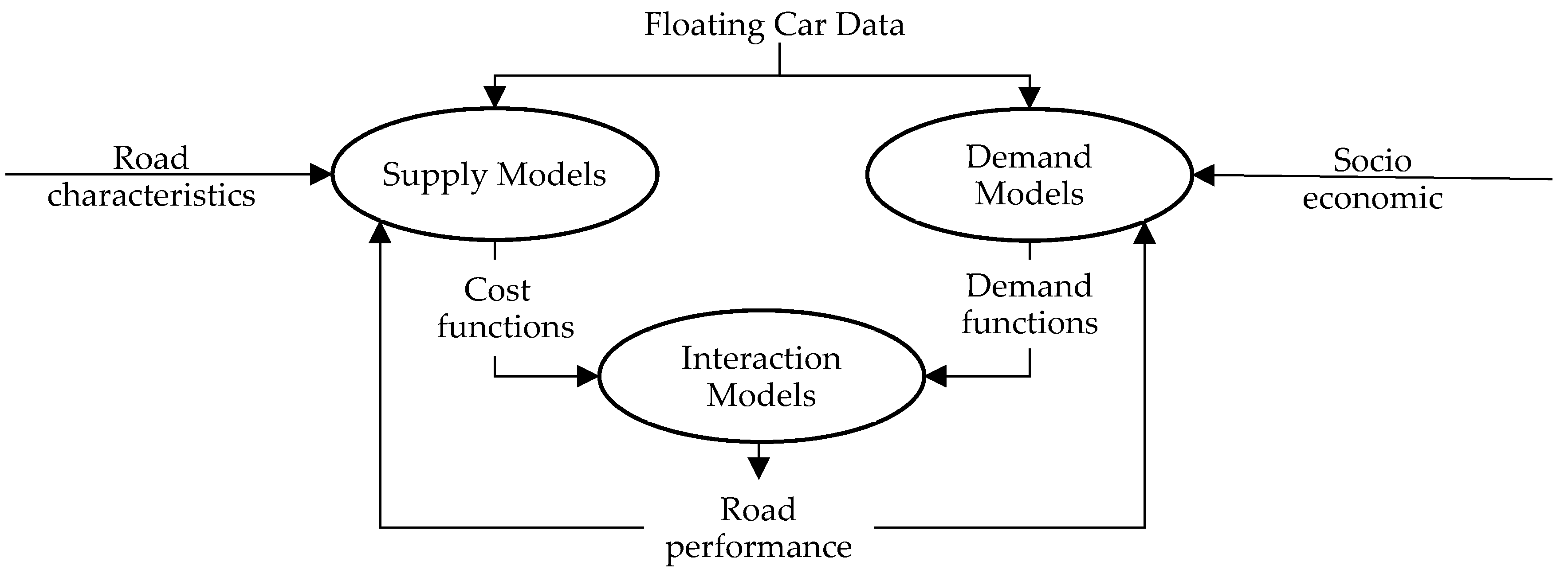
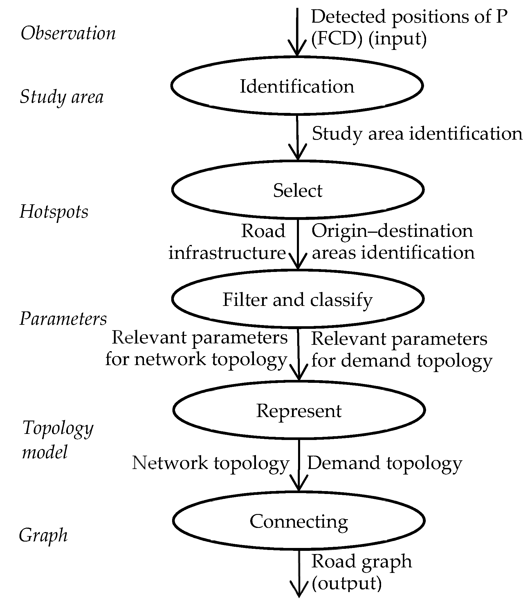
Generally, the following set of models are specified, calibrated and validated to build a TSM (Figure 1):

• transport supply models, to represent infrastructure, services and relative cost function, and topology (graph building);
• travel demand models, to represent mobility by means of demand functions;
• transport supply—travel demand interaction models, to represent how users choose supply components influencing their performances.

Starting from the observation data (input), the steps to build zones and road graph (output) according to traditional methods of transport systems engineering are:

• identification of the study area;
• regarding the supply model, it is necessary,

  ○

  to select the relevant road infrastructures;

  ○

  to filter and classify the linear (e.g., road links with homogeneous characteristics), nodal (e.g., road intersections and surface (e.g., parking areas) elements;

  ○

  to represent the topology of road network with the identification of nodes and links, building a road graph;

• regarding the demand model, it is necessary,

  ○

  to select the portions of study area with the highest potentials in terms of population emission/attraction;

  ○

  to filter and classify the relevant locations for the purpose of representing road mobility and to subdivide the study area into homogeneous areas, called zones;

  ○

  to represent the zones with centroids, and connect them to the road graph.

TSMs can be built using traditional procedures and data. It is necessary to identify supply (node and links) and demand (zones) components, in relation to a study area and to a temporal period. Big data (Input), in general and in the specific case of FCD, can support traditional methods in order to simulate the transport systems in a more representative way.

3.3. Transport System Models with Big Data

In order to integrate TMSs traditional procedures and FCD a procedure is proposed with specific reference to the graph building and zoning.

The procedure is organized in the following steps: Observation (Input); Study area (Identification); Hotspots (Select); Parameters (Filter and Classify); Topology model (Represent); Graph (Output).

Each step has its own aims, it is realized performing specific operations, and it supports one of the phases of traditional procedures. Operations of each step have a level of detail to be defined in relation to the transport planning dimension and to the relative required analyses. For instance, by considering study-in-depth planning dimension [25], the level of detail depends on the type of plan, ranging from the most aggregate (director) to the most disaggregate (feasibility). Different spatial planning dimensions (e.g., national, regional or local) require a different level of detail of the analyses.

In the following, each step is described in terms of the main aims, operations, and support related to each transport component: transport supply and travel demand. In some cases, a specification of traditional and advanced approaches with FCD is specified.

At this stage of the research, the procedure is proposed in relation to passengers’ mobility on a road network in an extended extra-urban area. In Figure 2 and

Table 1. Synthesis of the proposed procedure.

	INPUT
Observations	Aims	Visualising available detected positions (FCD)
	Operations	Mapping detected positions (FCD)
	Support	Preliminary study area delimitation
Study area	Aims	Visualising detected positions of P in the study area
	Operations	Iso-intensity curves of detected positions of P with r = ra and limit intensity
	Support	Study area identification
		SUPPLY		DEMAND
Hotspots	Aims	Representing roads		Representing origins-destinations of trips
	Operations	Iso-intensity of detected positions of P with r = rb		Iso-intensity of detected positions of P related to origin–destination of trips with r=rc
	Support	Road infrastructures selection		Origin–destination areas identification
Parameters	Aims	Estimating supply parameters		Estimating demand parameters
		Traditional	Advanced	Traditional	Advanced
	Operations	To quantify road width (L)	Frequency analyses to quantify road density threshold (ks)	To quantify area surface threshold (Sz)	Frequency analyses to quantify minimum intensity (Dmin) maximum intensity (Dmax)
	Support	Relevant parameters for network topology		Relevant parameters for demand topology
Topology model	Aims	Identifying nodes and links		Identifying zones and centroids
		Traditional	Advanced	Traditional	Advanced
	Operations	Types of roads classified according to road width (e.g., motorways, highways, local, …)	Classification of roads infrastructures Area (e.g., parking areas) Punctual (e.g., road intersections) Linear (e.g., road links)	Type of zones external internal with S < Sz internal with S < Sz	Classification of zones internal with high intensity (D ≥ Dmax) internal with medium intensity (Dmin ≤ D < Dmax) internal with low intensity (D < Dmin)
	Support	Network topology building: nodes and links		Demand topology building: zones and centroids
	OUTPUT
Graph	Aims	Building road graph and zones definition
	Operations	Connecting supply and demand topology
	Support	Road graph construction

there is a synthesis of the proposed procedure.

3.3.1. Observations (Input)

The aim of this step is to obtain a first qualitative visualization of detected positions of P (available GPS space-time coordinate) that, integrated with traditional data, are the input of the procedure. For these reasons, it is necessary to build a spatial map of Ps (operations).

Results of this step supports a preliminary study area delimitation.

3.3.2. Study Area (Identification)

The aim of this step is to analyze intensity of detected positions of P performing the following operations:

• to build a map of the values of intensity function of detected positions P, whose influence area has distance r_a [26];
• to build iso-intensity curves;
• to identify a limit intensity curve in order to identify a study area.

The final release of the study area results from a combination of advanced and traditional criteria (e.g., territorial boundaries). Results of this step supports study area identification that depends on the general purposes of the study.

3.3.3. Hotspots (Select)

The aim of this step is to analyze intensity of detected positions of P (for supply) and detected positions of P related to origin–destination of trips (for demand) inside the study area.

Starting from results of the previous step, considering the intensity function with specific distance:

• in relation to transport supply, operations consist on building iso-intensity curves of detected positions of P, whose influence area has distance r_b;
• in relation to travel demand, operations consist on building iso-intensity curves of detected positions of P, whose influence area has distance r_c.

It is worth noting that the values of r_a, r_b and r_c depend on general purposes of the analysis.

Results of this step supports the identification of relevant road infrastructures for transport supply estimation, and the identification of zones, which are origin–destination of trips (e.g., trip emission/attraction poles).

3.3.4. Parameters (Filter and Classify)

The aim of this step is to quantify parameters, which are required in the next step to identify the main elements of transport supply and travel demand.

In the traditional approach, a quantitative variable to select and classify relevant road infrastructures is the road width (L), capacity, flow, expressed for instance in meters; while another quantitative variable to define the extension of the zones is the surface (S), population, activities.

In the advanced approach, using FCD, starting from results of the previous step:

• in relation to transport supply, operations consist on performing a frequency analysis of vehicular density on the roads infrastructures, identifying a threshold value of vehicular density (k_s), depending on general purposes of the analysis;
• in relation to travel demand, operations consist on performing a frequency analysis of intensity of detected positions of P, identifying the following thresholds,

  ○

  a minimum intensity threshold of detected positions of P related to origin–destination of trips (D_min), that represent the lower bound value of intensity to identify aggregations of trip origins/destinations;

  ○

  a maximum intensity threshold of detected positions of P related to origin–destination of trips (D_max), that represent the upper bound value of intensity to identify aggregations of trip origins/destinations.

Results of this step supports the selection of relevant parameters to build network and demand topology.

3.3.5. Topology Model (Represent)

The aim of this step is to identify meaningful elements of supply and demand, and to classify them in relation to their functions in the transport system.

In the traditional approach:

• in relation to transport supply, operations consist on the identification of classes of roads according to their width (e.g., motorways, highways, local), by means of variable (L);
• in relation to travel demand, operations consist on the identification of the types of zones, considering a surface threshold (S_z),

  ○

  zones outside the study area;

  ○

  limited zones (with S < S_z) inside the study area;

  ○

  extended zones (with S ≥ S_z) inside the study area.

In the advanced approach, using FCD, starting from results of the previous step,

• in relation to supply, operations consist on identification of types of road infrastructures: area (e.g., parking areas); punctual (e.g., road intersections), or linear (e.g., road links);
• in relation to demand, operations consist on identification of the following the types of zones, considering intensity thresholds, D_min and D_max,

  ○

  internal zones with high intensity of detected positions of P related to origin–destination of trips (D ≥ D_max);

  ○

  internal zones with medium intensity of detected positions of P related to origin–destination of trips (D_min ≤ D < D_max);

  ○

  internal zones with low intensity of detected positions of P related to origin–destination of trips (D < D_min).

By combining the selection criteria deriving from traditional and advanced approaches, it is possible to identify different classes of internal zones. The final step of zones identification, and relative centroids, takes into account the criterion based on administrative boundaries (e.g., census areas where socio-economic data are available). For instance, in the case of extended zones inside the study area with low intensity of detected positions of P related to origin–destination of trips or limited zones inside the study area with high intensity of detected positions of P related to origin–destination of trips, it could be necessary to disaggregate an urban area limited by administrative boundaries.

Results of this step supports the identification of: network topology in terms of nodes and links; demand topology in terms of zones and relative centroids.

3.3.6. Graph (ConnectingOutput)

By connecting supply and demand topology (nodes, links, zones, and centroids), the graph and the connections with the zones are obtained. For this reason, it is necessary to identify fictitious links that represent connections between centroids and real nodes of road network.

4. Experimentation

The main objective of the experimentation is to validate the feasibility of the proposed procedure.

Experimentation consists in building elements of TSM, concerning road graph, zoning, and related connections. TSM is the basis for simulating passenger mobility in a study area, which is the backward (sub)-urban area near an Italian port. The port, called “Porto delle Grazie” in the Municipality of Roccella Jonica (Italy), is one of the most important marinas in the south of Calabria. The area near the port includes 16 municipalities with a total population of about 72,000 inhabitants and 14,200 employees.

The port has already acquired certifications about environmental sustainability. The goal is to increase sustainability by satisfying the demand of mobility to and from the port by means of electric vehicles, powered by renewable energy produced by sea waves. To this end, it is necessary to analyze the potential mobility between the port and other parts of the study area, focusing on mobility from and to cultural heritage.

4.1. Transport System Models

In a starting phase of the experimentation, TSMs are built with traditional methods, identifying supply and demand elements relative to road mobility in the study area. The traditional steps, described in Section 3.1 are executed [27]. In next section, the advanced steps are executed with the support of FCD data.

4.2. Transport System Models with Big Data

The advanced steps of the proposed procedure are aligned to the traditional steps, according to the description of Section 3. The starting data-base is composed of FCD data (geo-referenced temporal space positions of vehicles), extracted by a sample of vehicles equipped with GPS data logger.

FCD were recorded during a period of 4 non-consecutive weeks (1 week/month in the months of February, March, July, and August 2018). The data-base contains data about 19,547 vehicles, which represent about the 2% of all vehicles circulating in the province of Reggio Calabria, and it is composed of 5,311,407 records, where each record provides the detected positions of each road vehicle, P, collected during the observation weeks (

Table 2. Vehicles and detected points during the observation weeks.

	Province of Reggio Calabria		Area Near the Port
	Vehicles	Detected points	Vehicles	Detected points
Total numbers	19,547	5,311,407	7650	570,991

).

The procedure is applied through the following 6 steps, already described in Section 3.

4.2.1. Observations (Input)

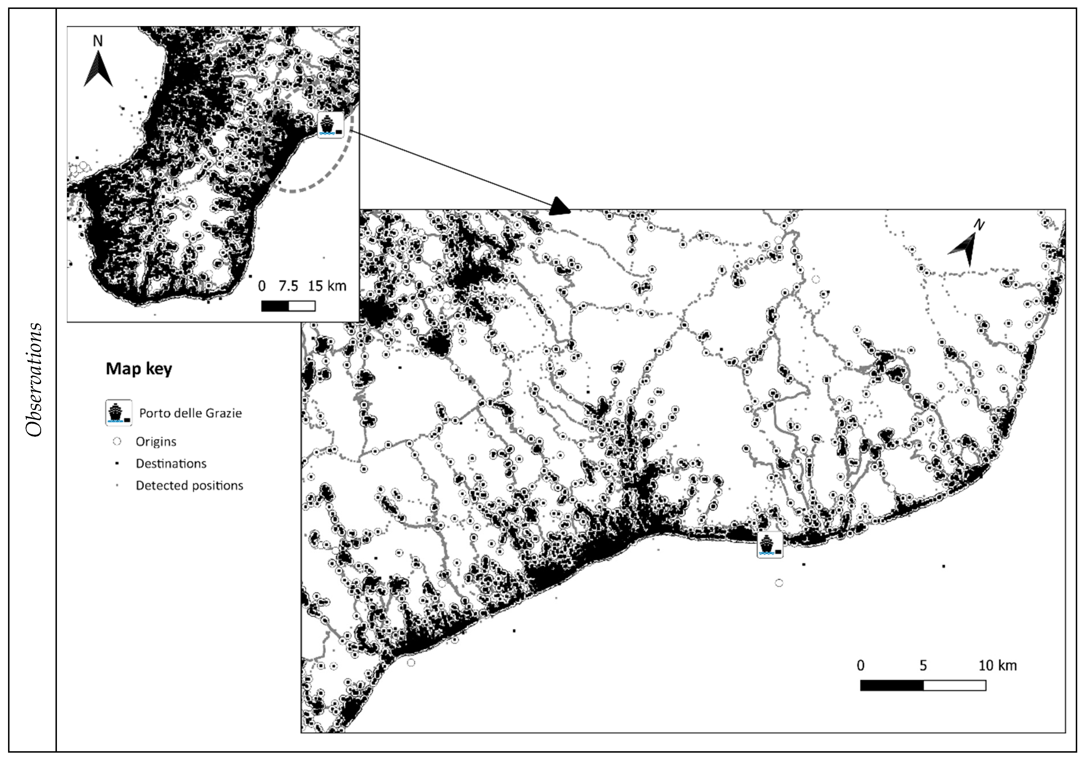
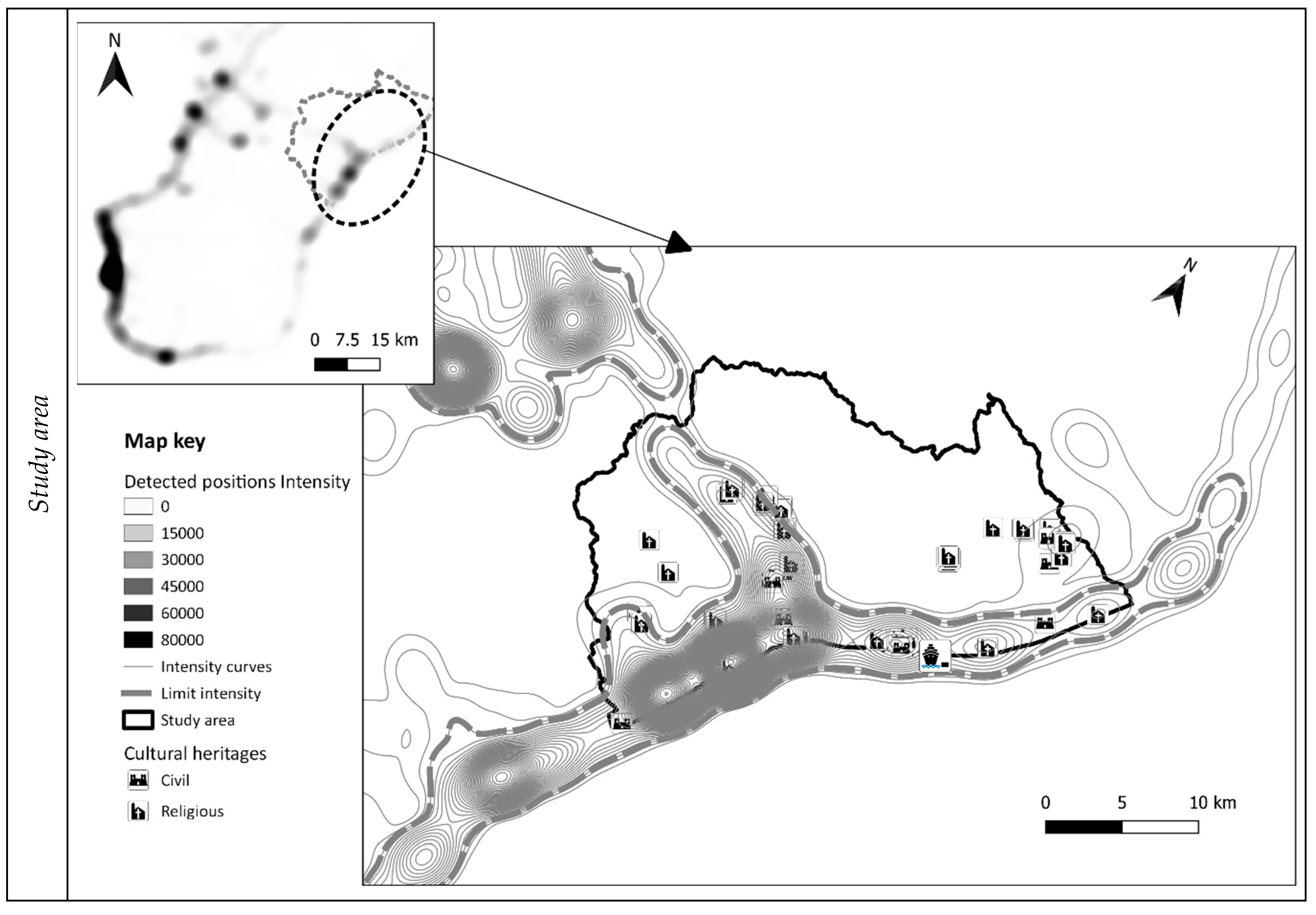
During the observation step, the whole detected positions of P (input data), were visualized on a geo-referenced map, with the aim of providing a preliminary idea of potential study area. Figure 3 shows the detected positions, P, inside the whole Province of Reggio Calabria (small map in the top-left of the figure) and in the area near the port (main map of the figure) during the period of analysis of 4 weeks. The detected positions, that are also origins and destinations of the trips, are represented with specific labels (see the map key). The portions of the area where there is the highest concentration of detected positions (black spots) are mainly present along the coast, where are located the main urban centres.

4.2.2. Study Area (Identification)

On the base of input data of the previous step, the influence areas of detected points P were calculated assuming a circular shape with constant radius r_a = 3 km (Figure 4, small map in the top-left of the figure) and with a linear decay function. The small map shows the different values of intensity for each geographical point using different greys from white (intensity = 0) to black (intensity > 8 × 10⁴). Afterwards, the iso-intensity curves were extracted to identify homogeneous areas, characterized by the same intensity values (main map of the figure). Figure 4 also shows the result of the application of the three criteria to identify the study area (see Section 3.3.2): (a) the value of limit intensity equal to 3000, (b) the areas with the highest concentration of cultural assets and (c) the administrative boundaries. The main map shows the iso-intensity curves with continues thin grey line, the limit intensity curves with dashed grey line, the boundary of the study area with continues black line.

4.2.3. Hotspots (Select)

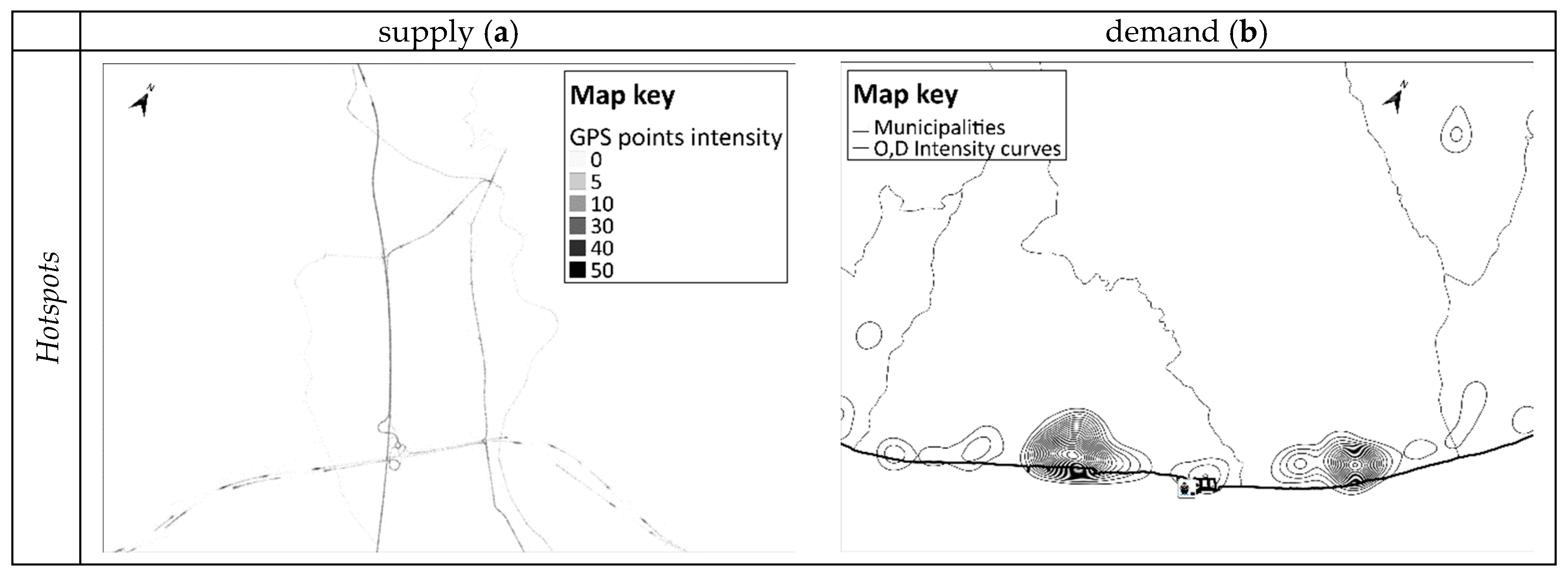
The visualization of the spatial distribution of detected positions of P allows to identifying the areas with the highest intensity (hotspot) for supply (road graph) and demand (zones). In order to identify the hotspots, an intensity function was used.

In relation to road graph, iso-intensity curves composed of all detected positions of P have been obtained with a circular influence area (r_b = 10 m) and a linear decay function.

Figure 5 (left map) illustrates the result of the procedure applied to a prototypal portion of the area, obtaining a selection of road infrastructures (links) that could be part of the road network, the one mostly used by the available set vehicles. The left map shows the different values of intensity for each geographical point using different scales of grey from white (intensity = 0) to black (intensity > 50). Results of these operations are links and relative nodes.

Similarly, for demand, iso-intensity curves of detected positions of P related to origin–destination of trips have been obtained with a different radius r_c = 565 m Figure 5 (right map) shows, for another prototypal portion of the area, the intensity curves of the origins/destinations of the vehicular trips, obtained as result of the trip processing of available set of vehicles. The right map shows the OD iso-intensity curves with continuous grey line, the boundary of the municipalities with continuous light grey line.

4.2.4. Parameters (Filter and Classify)

The traditional and advanced approaches (see Table 1) were jointly applied for the estimation of the parameters (thresholds), which are necessary for the identification of the main elements of supply and demand.

According to the traditional method, the selection of relevant infrastructures for the purpose of the analysis is based on the road width (L), while the selection of the areas depends on their surface (S).

According to the advanced method, the selection of relevant infrastructures depends on the frequency analysis of vehicular density on road infrastructures, and of the intensity thresholds for the zones.

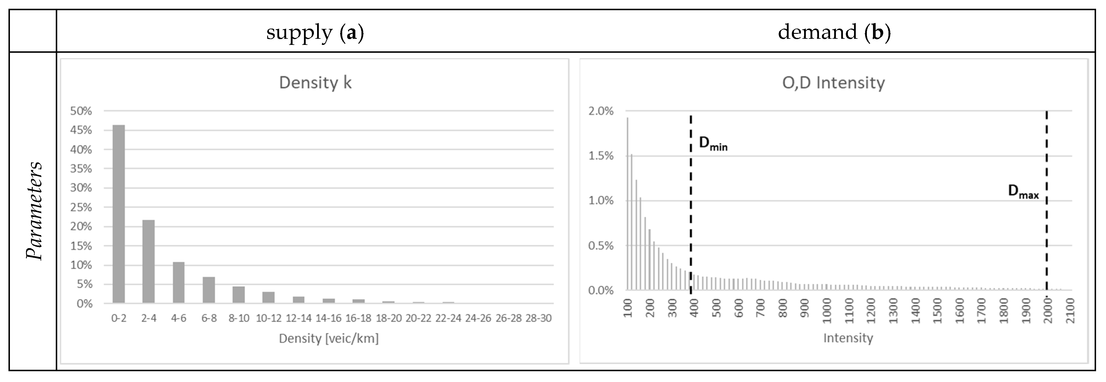
In the case of transport supply, a density threshold of 4 vehicles/km was identified, according on the purpose of the study.

For what concerns the intensity of origins/destinations, about 86% of the study area presents very low intensity values (less than 120), most trips are concentrated in the remaining part of the study area. Figure 6 shows the frequency histograms, respectively, of the vehicular density (a), and of the intensity of OD of trips (b) with the indication of the upper (D_max) and lower (D_min) thresholds.

In particular, the right histogram in Figure 6 shows that:

• about 7% of detected positions of P related to origin–destination of trips are concentrated in areas characterized by intensity values lower than 400,
• 5% in areas with intensity between 400 and 2000;
• 2% on areas with intensity greater than 2000.

Two intensity thresholds were identified:

• a minimum threshold D_min = 400;
• a maximum threshold D_max = 2000.

4.2.5. Topology Model (Represent)

In this step, the joint application of traditional and advanced approaches (see Table 1) as in the previous one, allows to identifying the main elements of the supply and demand model, as well as their classification in relation to their functions inside the transport system.

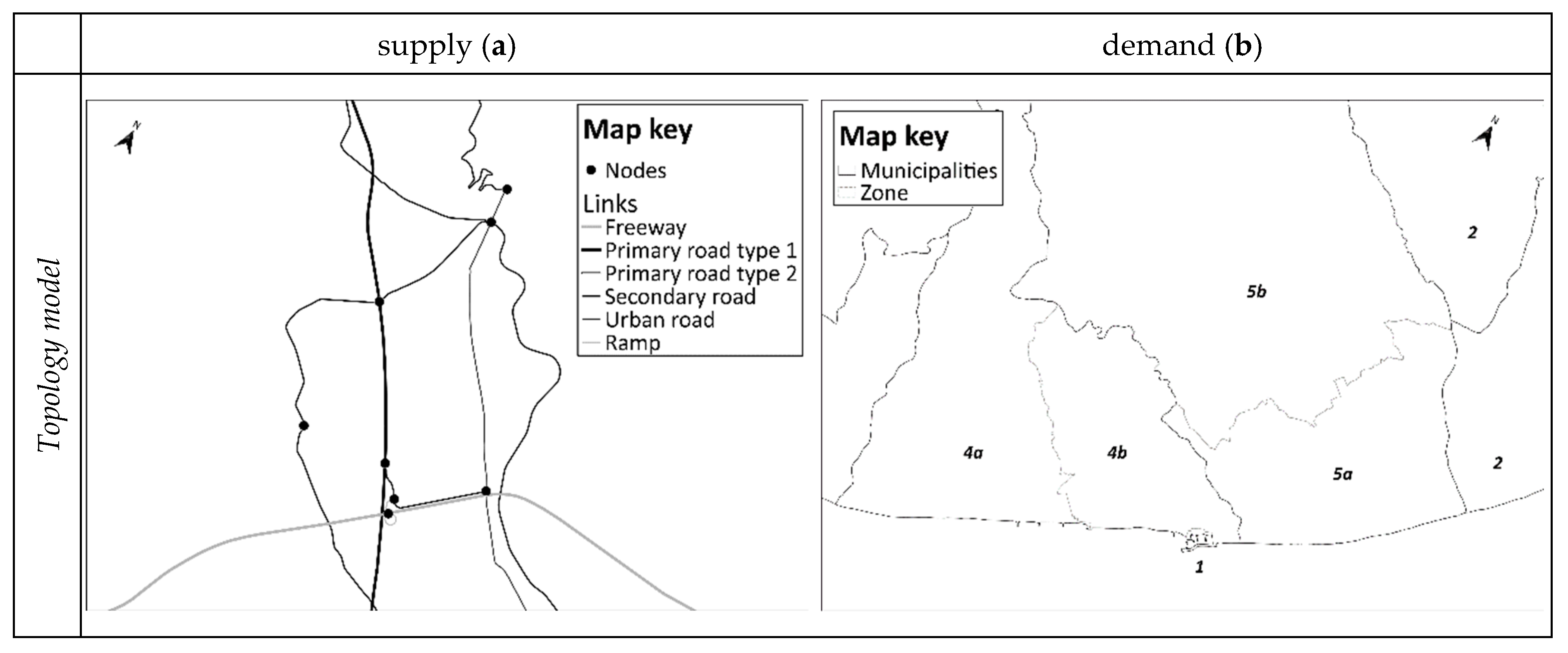
With the traditional approach, the supply elements (links) have been identified and classified into the following classes: (1) highways; (2) primary roads of type 1, separated carriageways; (3) primary roads of type 2, single carriageway; (4) extra-urban roads; (5) urban roads; (6) highway ramps.

Figure 7 (left map) illustrates the result obtained with the representation of the selected nodes and links. The map shows the different types of road links using different scales of grey.

The combination of the two criteria led to the identification of the following types of zones:

(1)

zones outside the study area;

(2)

zones inside municipalities with S < S_z and areas of intensity D < D_min;

(3)

zones inside municipalities with S < S_z and areas of intensity D_min ≤ D < D_max;

(4)

zones inside municipalities with S < S_z and areas of intensity D ≥ D_max;

(5)

internal zones in municipalities with S > S_z surfaces and areas of intensity D > D_min.

Municipalities with areas of type (4) and (5) were divided into smaller zones to better capture mobility inside the municipality. Figure 7 (right map) shows the zones obtained by applying the thresholds identified in the previous section inside a prototypal portion of the area. The map shows of different types of zones: type 1 (Porto delle Grazie); type 2 (municipalities of Stignano and Placanica); type 4 (municipality of Roccella Jonica); subdivided into two zones (4a and 4b); and type 5 (municipality of Caulonia), subdivided into two zones (5a and 5b).

4.2.6. Graph (Output)

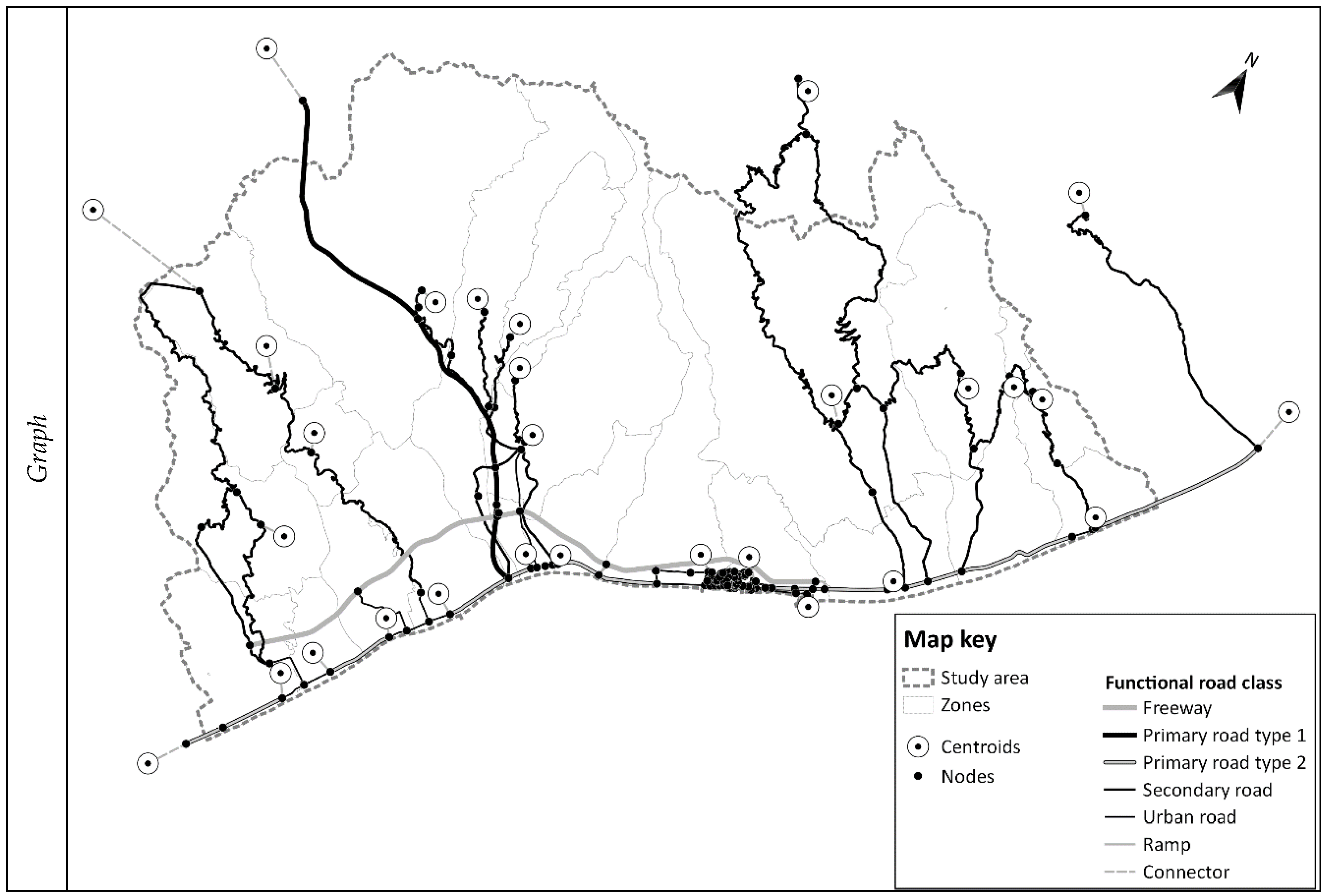
By connecting the elements identified by the topological model (previous step), as a result, the graph, the zones, the centroids, and the relative connectors are obtained. Figure 8 shows the results of the procedure related both to the supply, with the representation of nodes and of functional classes of links, and to the travel demand, with the representation of the zones and of the centroids. The study area consists of 23 zones, the road graph associated with is composed of 165 nodes and 210 road links, with a total length of 319 km.

5. Conclusions and Further Developments

Big data allow observing historical and current mobility patterns and transport facilities and services. In order to assess the a-priori effects and the costs and benefits of the forecasted scenarios of transport system, in it necessary to specify, calibrate and validate TSMs. While TSMs have become more sophisticated, the above model building protocol is still based, essentially, on travel diary surveys covering a small sample of the population (small data).

The study novelty regards the integration of big and small data in building (parts of) TSMs, with the aim to increase the capacity of transport analysts and planners to analyze, forecast and plan mobility phenomena. Traditional methods to build TSMs are enriched with big data for mobility.

In this regard, the procedure proposed follows the steps adopted by traditional methods of transport systems engineering to execute two operations: graph building, regarding transport supply; and zoning, for what concerns travel demand.

As far as concerns graph building, traditional methods of transportation researchers take into account the types of road elements classified mainly by road width (e.g., motorways, highways, and local). The contribution of big data, inside the proposed procedure, concerns the identification of the types of roads, according to the intensity of detected FCDs inside an area (of a given surface) or along a link.

For what concerns zoning, transportation researchers use traffic analysis zones, while big data analysts rely upon uniform grids or lattices. The procedure proposes to identify a zone using available big data (i.e., FCD), that is consistent with traditional methods based on small data on mobility patterns.

The experimentation of the proposed procedure concerned the process of zoning and of road graph building in an extra-urban area in the South of Italy. The practical application and the validation of the individual steps of the proposed procedure led the authors to the preliminary conclusion that it could produce potential benefits in terms of enhancement of model accuracy and costs reductions for surveys. Moreover, the procedure could be codified inside a GIS platform supporting transport planning.

Future research concerns developments of other TSMs components. FCD can support specification and calibration of cost and travel demand functions. Furthermore, FCD be useful in order to build supply-demand interactions models. Other developments concern in the extension of the study area in term of time period, spatial extension, urban areas.