Finding Visible kNN Objects in the Presence of Obstacles within the User’s View Field †

Abstract

In many spatial applications, users are only interested in data objects that are visible to them. Hence, finding visible data objects is an important operation in these real-world spatial applications. This study addressed a new type of spatial query, the View field-aware Visible k Nearest Neighbor (V2-kNN) query. Given the location of a user and his/her view field, a V2-kNN query finds data object p so that p is the nearest neighbor of and visible to the user, where visible means the data object is (1) not hidden by obstacles and (2) inside the view field of the user. Previous works on visible NN queries considered only one of these two factors, but not both. To the best of our knowledge, this work is the first to consider both the effect of obstacles and the restriction of the view field in finding the solutions. To support efficient processing of V2-kNN queries, a grid structure is used to index data objects and obstacles. Pruning heuristics are also designed so that only data objects and obstacles relevant to the final query result are accessed. A comprehensive experimental evaluation using both real and synthetic datasets is performed to verify the effectiveness of the proposed algorithms.

1. Introduction

The k nearest neighbor ($kNN$) query is an important spatial query type that has been studied extensively during the past decade [1,2]. Given a set of data objects and a query point q, a kNN query reports k data objects that are close to q. This kind of queries is useful in many real-world applications. For example, a tourist uses Google Maps to explore the restaurants that are closest to his/her location or a taxi driver utilizes the kNN query to find customers who are close to the taxi.

However, most existing works do not take the visibility of data objects into consideration, which makes their algorithms infeasible in many spatial applications; for example, interactive 2D online games, military simulation systems, and tourist recommendation systems.

Interactive 2D online games: In an interactive 2D online game, the overview map provides the enemy locations that can be seen from a player’s location. The player is interested in the map as the visible enemies are the main threat. Thus, the player should keep track of his/her nearest visible game objects so that he/she can attack or avoid them.

Military simulation systems: In a battle field, the command center wants to find one location to serve as the assembling point. Obviously, the assembling point should be clearly seen by the command center (i.e., it is not blocked by obstacles such as civilian buildings or vehicles), and the Euclidean distance from the command center to the assembling point should be minimized.

Tourist recommendation: A tourist information system provides k closest visible scenes for a given tourist. In this scenario, the scenes cannot be hidden by buildings or mountains so that the tourist can clearly see them in order to decide which one is his/her next visit point.

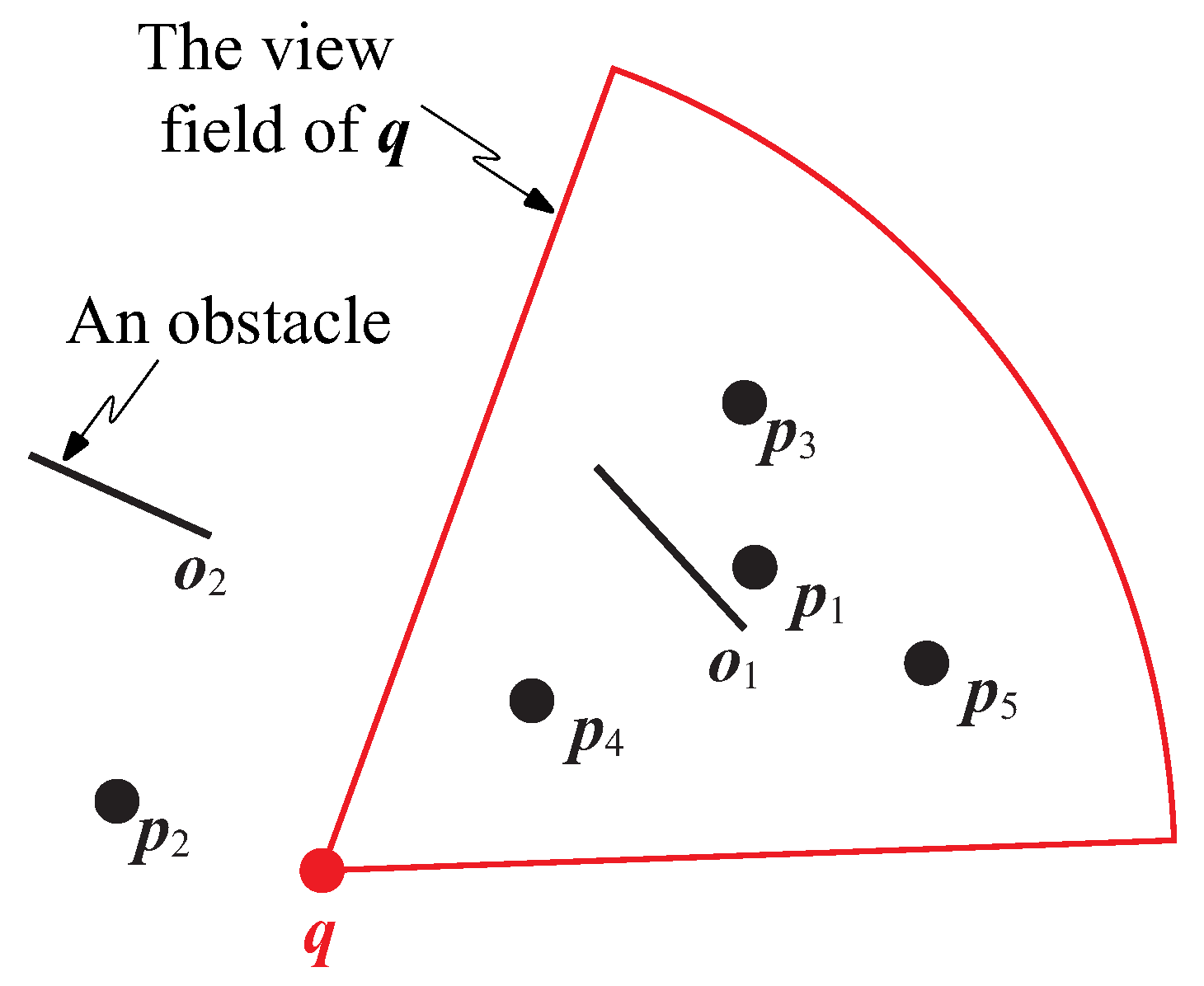
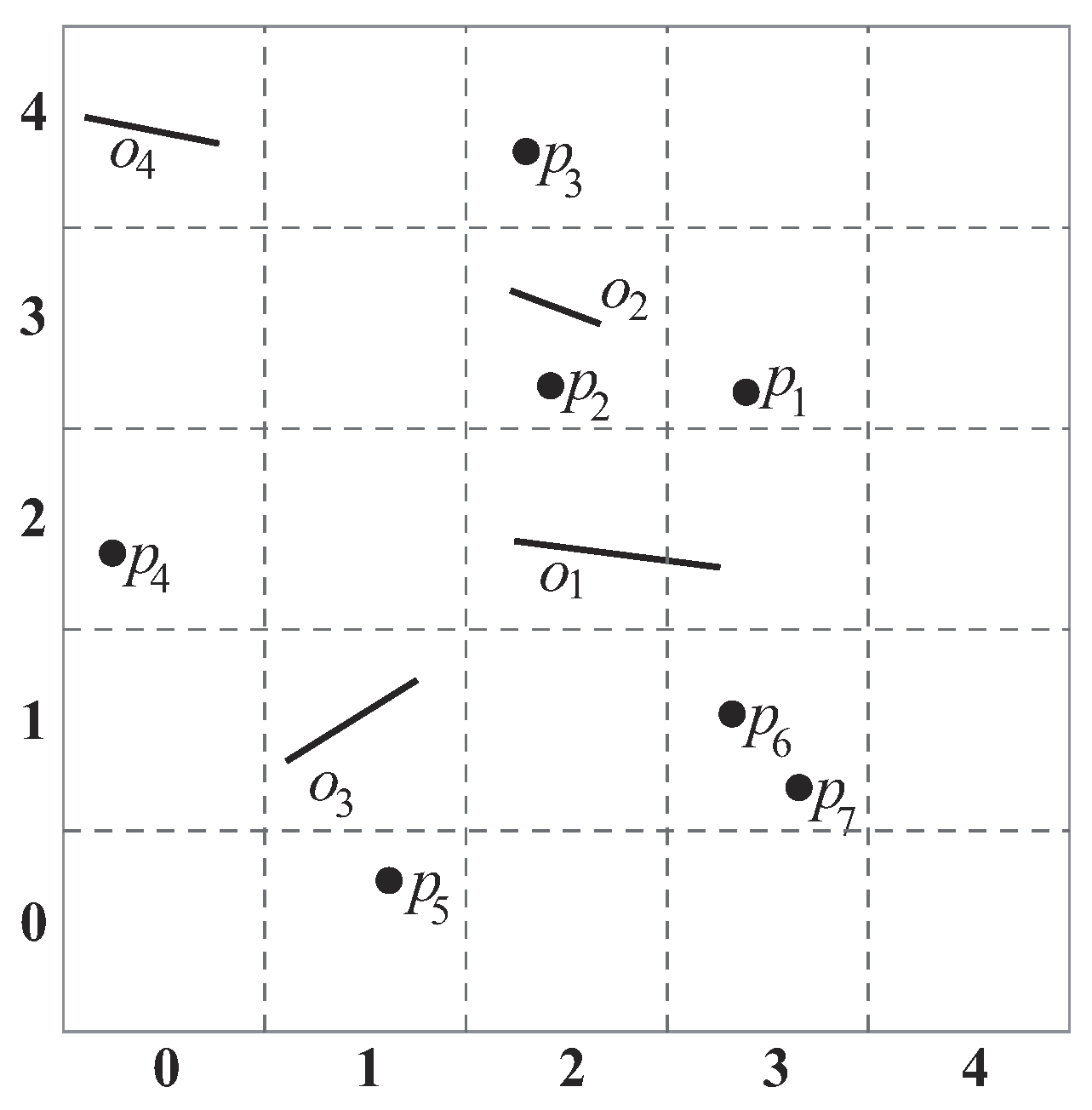
Conventional kNN query processing algorithms are inefficient for supporting current real-world applications as they do not take the visibility of data objects into consideration. This issue is illustrated in Figure 1, where q is the query point, $O=\{o_1,o_2\}$ are the obstacles (denoted by straight lines), and $P=\{p_1,p_2,p_3,p_4,p_5\}$ is a set of data objects. The fan-shaped area is the view field of query point q. Note that in this study, the visibility of a data object is affected by (1) the view field of a user and (2) the obstacles in the data space. The same as in [3], the view field defined in this paper is a 2D area that is the extent of the scene seen by a user; data objects are invisible to a user if they are outside his/her view field. Physical obstacles (e.g., building, trees, and hills) can block data objects so that they are invisible to the user [4].

Suppose $k=2$; the two visible nearest data objects of q are $p_4$ and $p_5$. Note that $p_2$ is the closest data objects for q in the conventional kNN retrieval. However, it is neglected in visible kNN applications as it is not within q’s view field. Furthermore, although $p_1$ is closer to q than $p_5$, it is not in the result set as $p_1$ is invisible to q owing to obstacle $o_1$.

To process such kinds of queries, an intuitive thought is to utilize the conventional kNN algorithms to find the solutions. Hence, a simple approach is to set a very large m value ($m>k$) so as to make sure that the “real answers” are included in the result set. However, a serious problem is that it is very difficult to decide on a proper m value. If m is too small, k visible NNs may not be identified; in this case, a new $m^{\prime }$ value ($m^{\prime }>m$) has to be chosen, and the search is repeated. This can result in redundant computations as many data objects are re-evaluated during the execution iterations. On the other hand, if m is too large, time is wasted in checking data objects that are not included in the final answer, leading to expensive I/O costs and computational overhead. Hence, a completely new method has to be devised to address this v2-kNN problem.

Related work of this research will be discussed in Section 2. Major challenges in processing the View field-aware Visible k Nearest Neighbor (V2-kNN) queries are (1) how to efficiently identify data objects and obstacles inside a given view field and (2) how to determine the visibility of a data object as fast as possible. If every data object p is accessed and compared with all the obstacles to determine whether p is inside the given view field, the I/O cost, as well as the computation time must be extremely high.

To address this problem, we propose an efficient algorithm to retrieve the visible data objects in a given view field. The algorithm checks the data objects from near to far (according to their distance from the query point), because nearer data objects are more likely to be included in the result set. In addition, we also develop a set of pruning heuristics so that only the obstacles highly relevant to the query result are accessed when the visibility check is performed. Finally, we conducted extensive experiments using both real and synthetic datasets to verify the effectiveness of our algorithms.

The manuscript is an extended version of our previous report [5], in which we introduced the V2-kNN problem and outlined the idea of our basic method. Here, we substantially extend the basic method to a much more sophisticated algorithm, which includes three smart pruning techniques and efficient techniques to further enhance the performance of the algorithm (see Section 4.2, Section 4.3 and Section 4.4). Other augmentations are include in Section 2, and we give a quite thorough review of related work to make the paper self-contained. In Section 3, we add several examples to explain the meaning of the notations. Furthermore, we conduct a comprehensive performance evaluation in Section 5.

The rest of the work is organized as follows. In Section 2, we review some related studies. We formalize the V2-kNN problem and introduce our index scheme in Section 3. In Section 4, we give the detailed description of the proposed algorithm. We also introduce the pruning techniques in the section. Results of our experimental study are reported in Section 5. Finally, Section 6 gives the conclusions and future research directions.

2. Related Work

kNN query processing is a hot research topic in the database community [1,2,4,6,7,8,9,10,11,12,13,14,15,16,17,18,19,20,21,22,23,24,25,26,27]. Numerous algorithms and data structures (e.g., B-tree [26], grid structure [27], or R-tree [28]) have been proposed for kNN query processing. Only a few of them are capable of processing “visible” kNN queries [4,14,15,18,19,20,21,22,23,24,25]. We can classify these works into two types: (1) visible kNN queries with the obstacle constraint and (2) visible kNN queries with the view field constraint. We will briefly review each of them in the following. Note that as we have mentioned in the previous section, none of these works consider the effect of obstacles and the view field at the same time.

2.1. Visible kNN Queries with the Obstacle Constraint

The VkNN query as proposed by Nutanong et al. [14,15]. A VkNN query retrieves k visible objects with the smallest distance to a query point q. Figure 2 shows an example of a VkNN query. In the figure, there are five data objects (i.e., $a,b,\cdots e$) and a query point q. The VkNN of q is $\{b,d\}$ (in order of their distance to q). Note that although a is the closest data object to q, it is not a qualifying answer. The reason is that a is hidden by an obstacle, and thus, it is invisible to q.

In [14,15], all data objects were indexed in an R-tree [28]. Nutanong et al. proposed two algorithms, POSTPRUNING and PREPRUNING, for processing VkNN queries. The difference between these two algorithms is the pruning strategies. The two algorithms are based on the observation that to check the visibility between q and data object p, we only need to compare p with the obstacles that are nearer to q than p.

Gao et al. in [4] studied the problem of continuously reporting visible k nearest neighbors to a query point moving along a line segment, whereas all the data objects are static. The algorithm utilizes R-tees to index the dataset and the obstacle set and uses a branch-and-bound technique to process the query. Gao et al. also proposed several pruning heuristics to improve the query performance. Another work that focused on continuously determining visible k nearest neighbors was proposed by Wang et al. [20]. They proposed a filtering-and-refinement framework to process the query efficiently. In the filtering stage, the authors proposed two pruning strategies to reduce the search space. Then, in the refinement stage, the algorithm examines the exact positions of the unfiltered data objects and finds the final result.

In [29], Wang et al. introduced All-k-Nearest-Neighbor (AkNN) search. Given a set of data objects P and a query set Q, an AkNN query finds for each query $q\in Q$ its k visible nearest neighbor in P. A naive method to tackle the problem is to perform the VkNN search for each query in Q. However, the method is inefficient as it needs to access the data objects in P many times, leading to high I/O and CPU costs. Wang et al. developed two algorithms to efficiently process AkNN queries. They also designed several pruning techniques to improve the query performance.

The Group Nearest Neighbor (GNN) query [16,17] is a novel form of NN search, which returns a data object with the minimum aggregate distance to all query points. For example, a group of friends, located at different places in a city, wants to find a restaurant for a meeting. The location of the restaurant should minimize the total travel distance to all the members in the group. The authors in [18,19] extended the idea of the GNN query by taking obstacles into account. Both of the works developed efficient pruning methods to prune unnecessarily accessed obstacles so as to enhance the query processing performance. The algorithms proposed in [18] can only handle the SUMaggregate function. However, in [19], the algorithm works for SUM, MIN, and MAXaggregate functions.

Gao et al. [30,31] introduced the Visible Reverse k Nearest Neighbor (VRkNN) query, which considers the obstacle influence on the visibility of data objects. They proposed the Visible Region Computation (VRC) algorithm to efficiently retrieve obstacles that affect the visibility of the query point. The VRkNN query processing algorithm utilizes the VRC algorithm to prune the search space and enhance the performance.

2.2. Visible kNN Queries with the View Field Constraint

The Nearest Surrounder (NS) query was proposed by Lee et al. [21,22]. An NS query retrieves the nearest neighbor objects for all orientations around the query point q. For example, in Figure 3a, data objects $O_1,O_2,\cdots ,O_6$ (i.e., the white rectangles) are the nearest surrounder objects of q. Note that $O_7,O_8,$ and $O_9$ (i.e., the gray rectangles) are not included in the answer set as they are hidden by other data objects.

For many applications, the data objects inside a certain view field are needed. The authors further proposed an NS query variant, named the Angle-constrained NS (ANS) query, which retrieves NS objects residing in a specified view field. In Figure 3b, an ANS query issued at q returns $\{O_3,O_5\}$. The major difference between (A)NS and V2-kNN is that the (A)NS query retrieves “all visible” data objects in the view field. However, on the other hand, the number of visible data objects returned by the V2-kNN query is specified by the k value.

Yi et al. [23,24] introduced the View Field Nearest Neighbor ($VFNN$) query that can retrieve the closest visible data object residing in a user’s view field. In [23], the authors used R*-tree [32] to index data objects and develop a branch-and-bound search algorithm to traverse the R*-tree to find the results. They also designed a pruning technology that can efficiently filter the R*-tree nodes that do not overlap with the given view field to enhance the search performance. In [24], Yi et al. designed a new algorithm to process the VFNN query. The new algorithm proposed in [24] uses a grid-based index to maintain data objects. The main difference between our approach and that of Yi et al. is that they did not take the effect of obstacles into consideration.

In [25], Yi et al. introduced the Reverse View Field Nearest Neighbor (RVFNN) query, which returns the nearest object (according to a query point) from among the data objects whose view fields contain the query point. The authors first proposed an algorithm that runs on R*-tree to process the RVFNN query. Then, they introduced a new type of spatial data index structure called the view field R-tree for RVFNN searches to overcome the limitations of R*-tree.

The hidden-surface determination problem [33] studied in the area of computer graphics shares some similarity to our problem. The hidden-surface determination is a process used to determine which surfaces and parts of surfaces are not visible from a certain viewpoint. Z-buffering [34] is one of algorithms that can address the problem.

When rendering a data object, z-buffering scans each pixel of the data object and projects it on a projection plane that faces a query point. Thus, only the pixels on the projection plane are visible to the user. For instance, in Figure 4, Point A is not projected on the projection plane since it is hidden by Point B. However, Point C is visible to the user.

Our problem and image rendering are conceptually and functionally different. Our work aims to design efficient mechanisms for finding visible objects from a very large set of data objects. Thus, how to design the index that facilitates faster data retrieval and how to develop pruning strategies that reduce the search space are the main concerns of the work. One the other hand, the image-rendering algorithm assumes that the data objects inside the view field are known in advance. The main jobs of the image rendering are how to improve the result accuracy and how to reduce the memory consumption.

3. Preliminary

In this section, we define several terms that are used in the work. We also formulate the V2-kNN search and present our index scheme for the processing of V2-kNN queries. We summarize the symbols used in the following discussion in

Table 1. Summary of symbols.

Symbols	Meanings
$(l,r,\theta )$	The location, the maximum visible distance, and the view field angle of q
${\theta }_q^{⊢}$	The starting angle of q based on the positive x-axis
${\theta }_q^{⊣}$	The ending angle of q based on the positive x-axis
$dist(p,q)$	The Euclidean distance between q and p
${\theta }_{q,o.min}$	The minimum angle between q and o
${\theta }_{q,o.max}$	The maximum angle between q and o
$MinDist(q,o)$	The minimum distance between o and q
$MaxDist(q,o)$	The maximum distance between o and q
$V_d$	The visible distance
C	A grid cell
$MinAngle(q,C)$	The minimum angle between query q and cell C
$MaxAngle(q,C)$	The maximum angle between query q and cell C
H	A min-heap that sorts accessed cells according their minimum possible distance to q
$RL$	A min-heap that maintains candidate query results
$OL$	A min-heap that retains already accessed obstacles
$best\_dist$	The current visible distance of the $k^{\mathrm{th}}$ visible data object of q
$C_{cur}$	The current cell
$VCL$	A visited cells list
${\theta }_{\mathcal{S}}$	A splitting angle
${\theta }_{IRLB}$	The splitting angle in the Invisible Regions Lookup Buffer (IRLB)
$Regio{n}_i$	The $i^{\mathrm{th}}$ region, which is split in IRLB

.

3.1. Problem Definition

In a two-dimensional Euclidean space, there are a set of data objects P = $\{p_1,p_2,p_3,...p_i\}$ and a set of obstacles O = $\{o_1,o_2,o_3,...o_j\}$. In this paper, we assume each obstacle is a line segment. Although an obstacle o may be an arbitrary convex polygon (e.g., triangle), we assume o is a line to simplify our discussion. The proposed algorithms can work with o of an irregular shape by treating o as a set of line segments.

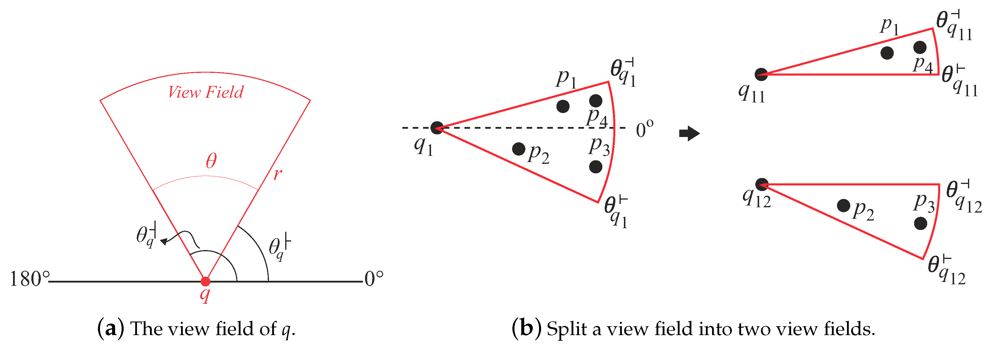
Definition 1.

Query point and its view field

A query point q is represented as a triplet $(l,r,\theta )$, where $l=(x,y)$ denotes the location of q, r denotes the maximum visible distance of a user, and θ is the view field angle of q. Note that $\theta =({\theta }_q^{⊢},{\theta }_q^{⊣})$ is a combination of two angles ${\theta }_q^{⊢}$ and ${\theta }_q^{⊣}$, where ${\theta }_q^{⊢}$ and ${\theta }_q^{⊣}$ are the values of the starting and ending angles based on the positive x-axis (see Figure 5a) (the definitions of starting and ending angles were adopted from [24]).

Also note that ${\theta }_q^{⊢}$ and ${\theta }_q^{⊣}$ must be in a continuous range between $[0^{\circ }$ - ${360}^{\circ }]$, i.e., $0^{\circ }\le {\theta }_q^{⊢}\le {\theta }_q^{⊣}\le {360}^{\circ }$. If ${\theta }_q^{⊢}$ is bigger than ${\theta }_q^{⊣}$, it must be a view field crossing from the first quadrant to the fourth quadrant of the coordinate space. For example, Figure 5b depicts a view field with ${\theta }_q^{⊢}$ = ${300}^{\circ }$ and ${\theta }_q^{⊣}$ = ${20}^{\circ }$. In this case, we will separate this view field into two parts. In Figure 5b, $q_1$ is split into $q_{1,1}$ and $q_{1,2}$ where ${\theta }_{q_{1,1}}^{⊢}=0^{\circ }$, ${\theta }_{q_{1,1}}^{⊣}={20}^{\circ }$, ${\theta }_{q_{1,2}}^{⊢}={300}^{\circ }$, and ${\theta }_{q_{1,2}}^{⊣}={360}^{\circ }$. When processing $q_1$, our algorithm will separately evaluate $q_{1,1}$ and $q_{1,2}$ and then merge the results. Thus, in Figure 5b, our algorithm returns $\{p_2,p_1\}$ to the user after it merges the results of $q_{1,1}$ (i.e., $\{p_1,p_4\}$) and $q_{1,2}$ (i.e., $\{p_2,p_3\}$).

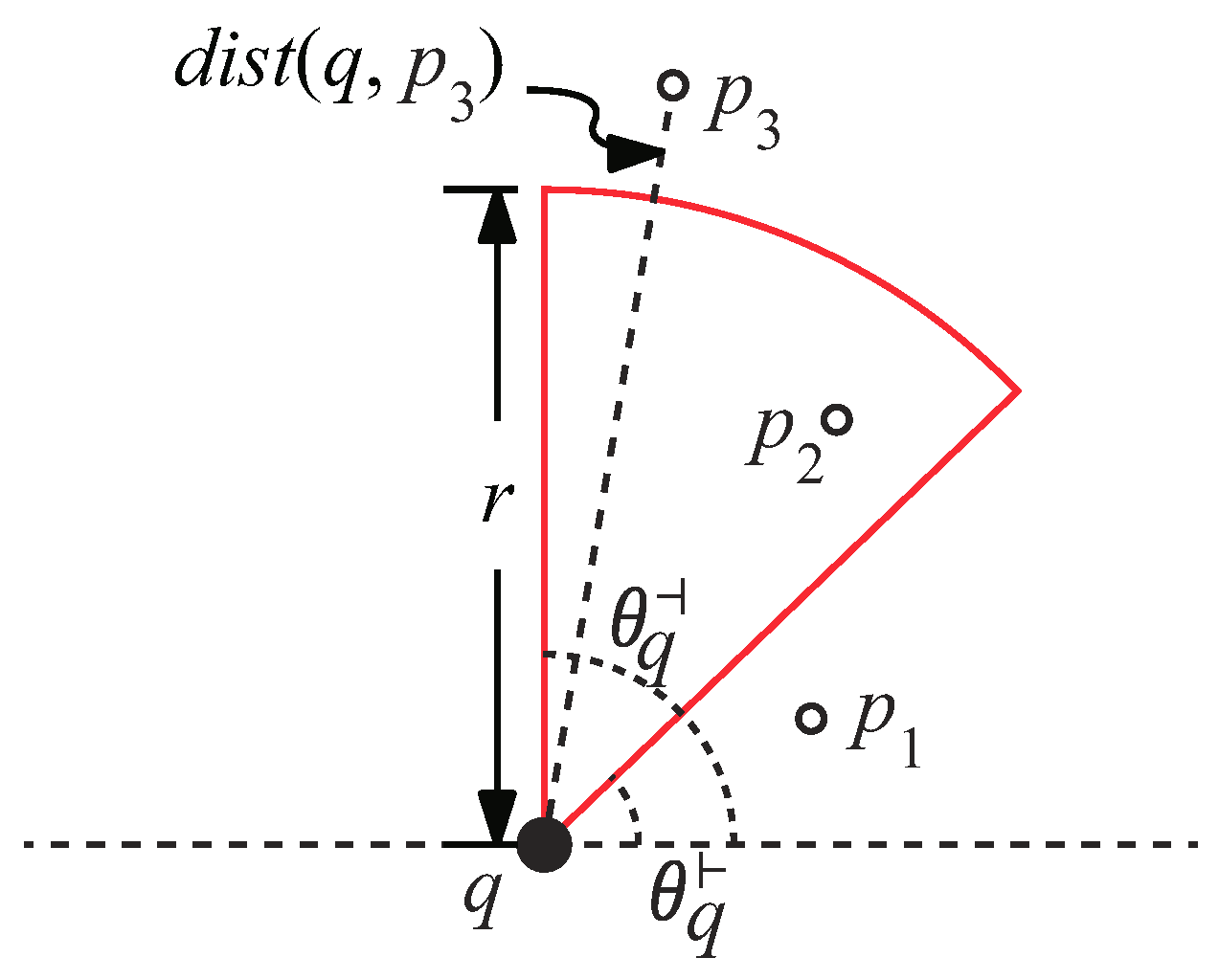
Now, we explain how to determine whether a data object or an obstacle is inside a view field or not. Given a data object p, we define $dist(p,q)$ to be the Euclidean distance between q and p and ${\theta }_{p,q}$ to be the angle between the positive x-axis and the vector $\overrightarrow{pq}$. Then, p is inside q’s view field if (1) ${\theta }_q^{⊢}\le {\theta }_{q,p}\le {\theta }_q^{⊣}$ and (2) $dist(q,p)\le r$ [24]. In Figure 6, $p_1$ is not inside the view field as ${\theta }_{q,p_1}>{\theta }_q^{⊢}$. For $p_3$, it is outside the view field because $dist(q,p_3)>r$.

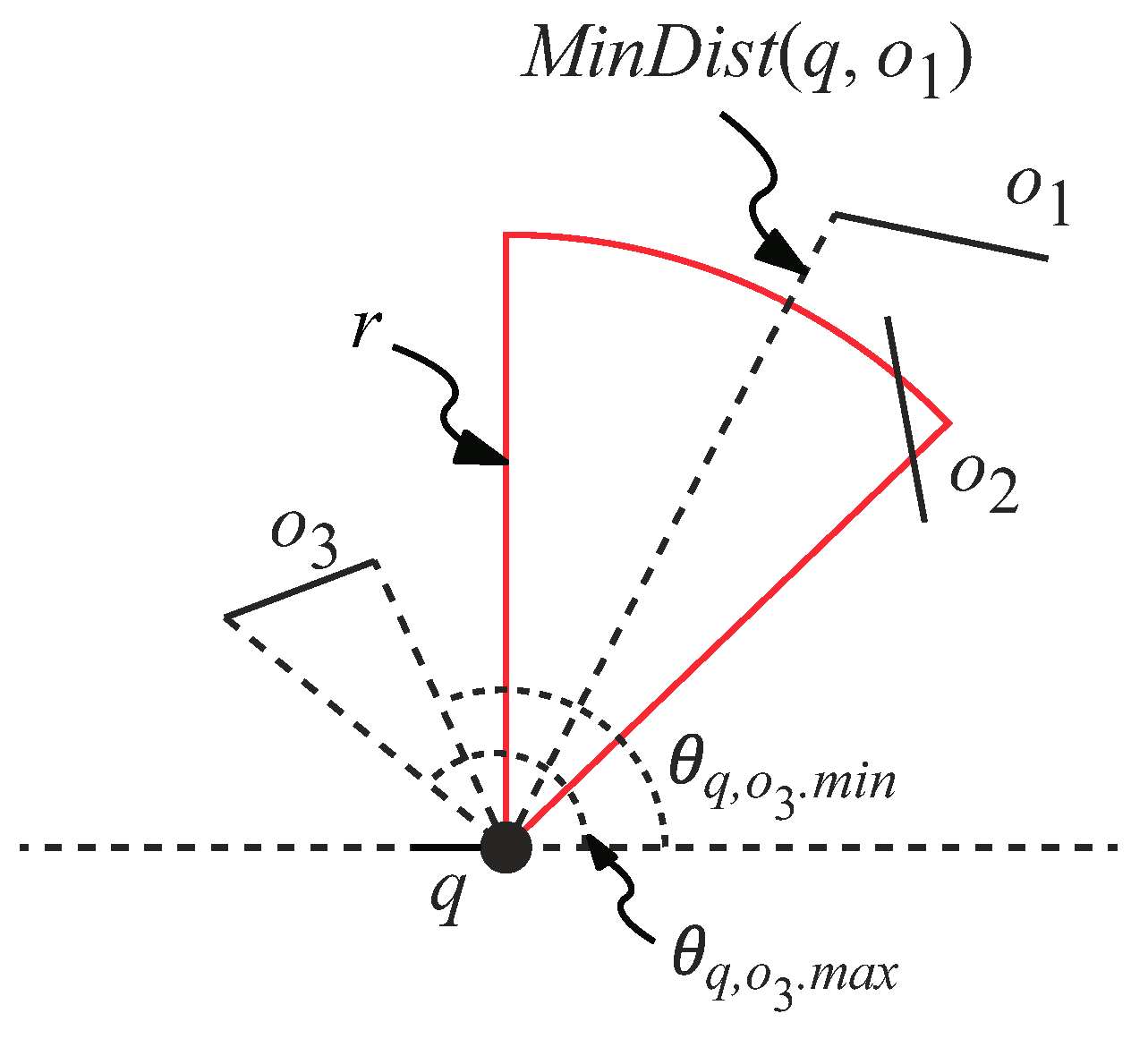
To explain how to evaluate whether an obstacle o is inside the view field, we first define some terms. We use (${\theta }_{q,o.min}$, ${\theta }_{q,o.max}$) to represent the angular bound of o’s line segment w.r.t. q, where ${\theta }_{q,o.min}$ denotes the minimum angle and ${\theta }_{q,o.max}$ denotes the maximum angle [31]. We also use $MinDist$(q, o) and $MaxDist$(q, o) to denote the minimum and maximum distance between o and q, respectively. An illustration of ${\theta }_{q,o.min}$, ${\theta }_{q,o.max}$, $MinDist$(q, o), and $MaxDist$(q, o) is shown in Figure 7.

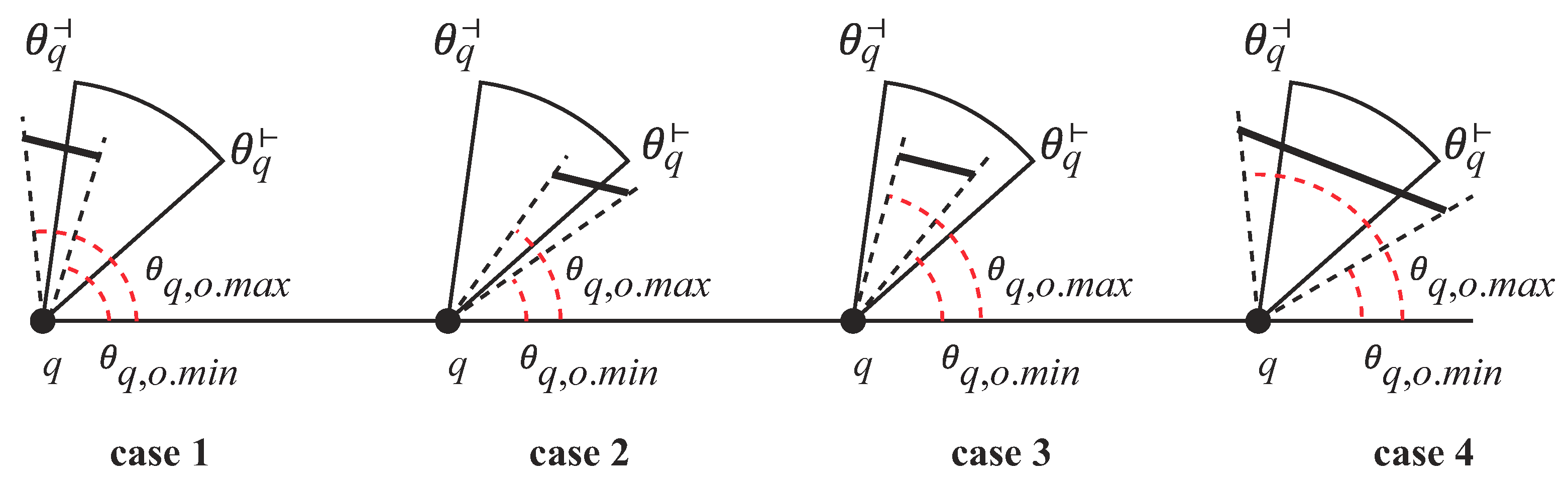
Given an obstacle o and a query object q, if o resides in q’s view field, then o satisfies (1) the minimum distance between q and o must be less than or equal to r (i.e., $MinDist(q,o)\le r$), and (2) the relationship among ${\theta }_q^{⊢},{\theta }_q^{⊣}$, ${\theta }_{q,o.min}$ and ${\theta }_{q,o.max}$ meets one of the following conditions:

• ${\theta }_q^{⊢}\le {\theta }_{q,o.min}\le {\theta }_q^{⊣}$and${\theta }_{q,o.max}>{\theta }_q^{⊣}$ (Case 1 in Figure 8),
• ${\theta }_q^{⊢}\le {\theta }_{q,o.max}\le {\theta }_q^{⊣}$and${\theta }_{q,o.min}<{\theta }_q^{⊢}$ (Case 2 in Figure 8),
• ${\theta }_q^{⊢}\le {\theta }_{q,o.max}\le {\theta }_q^{⊣}$and${\theta }_q^{⊢}\le {\theta }_{q,o.min}\le {\theta }_q^{⊣}$ (Case 3 in Figure 8),
• ${\theta }_{q,o.max}>{\theta }_q^{⊣}$and${\theta }_{q,o.min}<{\theta }_q^{⊢}$ (Case 4 in Figure 8).

In Figure 9, $o_2$ is inside the view field (i.e., Case 4). On the other hand, $o_1$ is not in the view field because $MinDist(q,o_1)>r$. $o_3$ is also outside the view field as ${\theta }_{q,o_3.min}>{\theta }_q^{⊣}$ and ${\theta }_{q,o_3.max}>{\theta }_q^{⊣}$. Similar to the view field, the obstacle $o_1$ is split into two obstacles $o_{1,1}$ and $o_{1,2}$ if o crosses the first and the fourth quadrants in the coordinate space.

Now, we formally define the visibility of data objects.

Definition 2.

Visibility of data objects

Given a query $q(l,r,\theta )$, a set of data objects $P=\{p_1,p_2,\cdots ,p_i\}$, and a set of obstacles $O=\{o_1,o_2,\cdots ,o_j\}$, a data object $p\in P$ is visible to q if all the following conditions are satisfied: (1) p is inside q’s view field. (2) There is no obstacle $o\in O$ between the straight line connecting q and p (denoted as $\overline{qp}$).

In addition, to represent the distance between two objects, taking visibility into consideration, we define the visible distance $V_d$ as follows:

Definition 3.

Visible distance[20]

Given a query q and a data object p, if p is visible to q, the visible distance between q and p (denoted as $V_d(q,p)$) is the minimum Euclidean distance between them (i.e., $dist(q,p)$). Otherwise, $V_d(q,p)$ is set as infinite. That is,

$$V_d(q,p)=\left\{\begin{array}{cc}dist(q,p)\hfill & ifpisvisibletoq,\hfill \\ \infty \hfill & otherwise.\hfill \end{array}\right.$$

(1)

After giving the definitions of the view field, visibility, and the visible distance, we can formally define our problem:

Definition 4.

View-Field-aware Visible k Nearest Neighbor (V2-kNN) search problem

Given a query $q(l,r,\theta )$, a set of data objects $P=\{p_1,p_2,\cdots ,p_i\}$, and a set of obstacles $O=\{o_1,o_2,\cdots ,o_j\}$, a view-field-aware visible k nearest neighbor query retrieves a subset of P, denoted by $V2$-$kNN(q)$, such that:

• $|V2$-$kNN(q)|=k$;
• $\forall p\in V2$-$kNN(q)$, p is visible to q;
• $\forall p\in V2$-$kNN(q)$ and $p^{\prime }\in P\setminus V2$-$kNN(q)$, $V_d(q,p)\le V_d(q,p^{\prime })$.

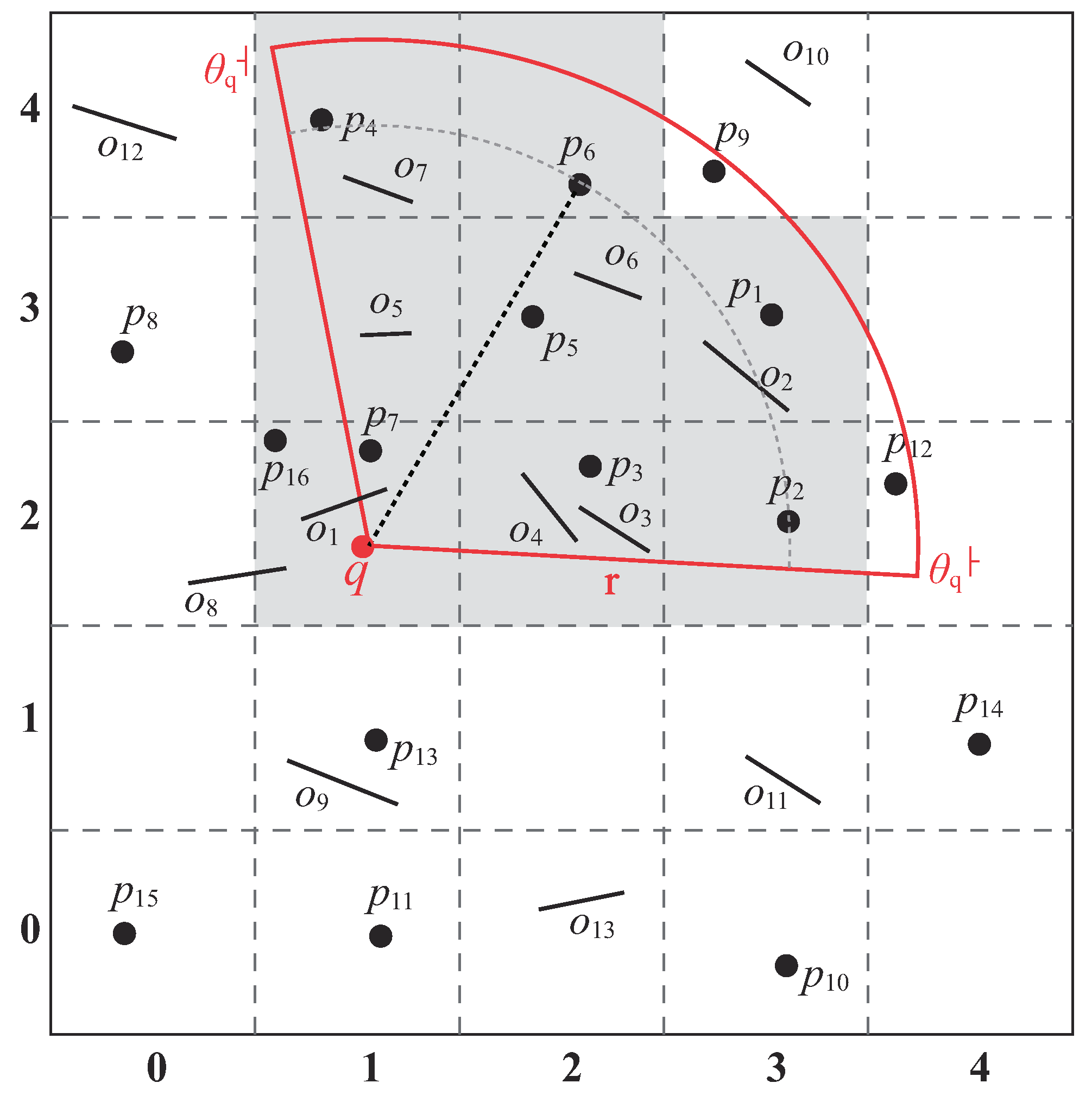
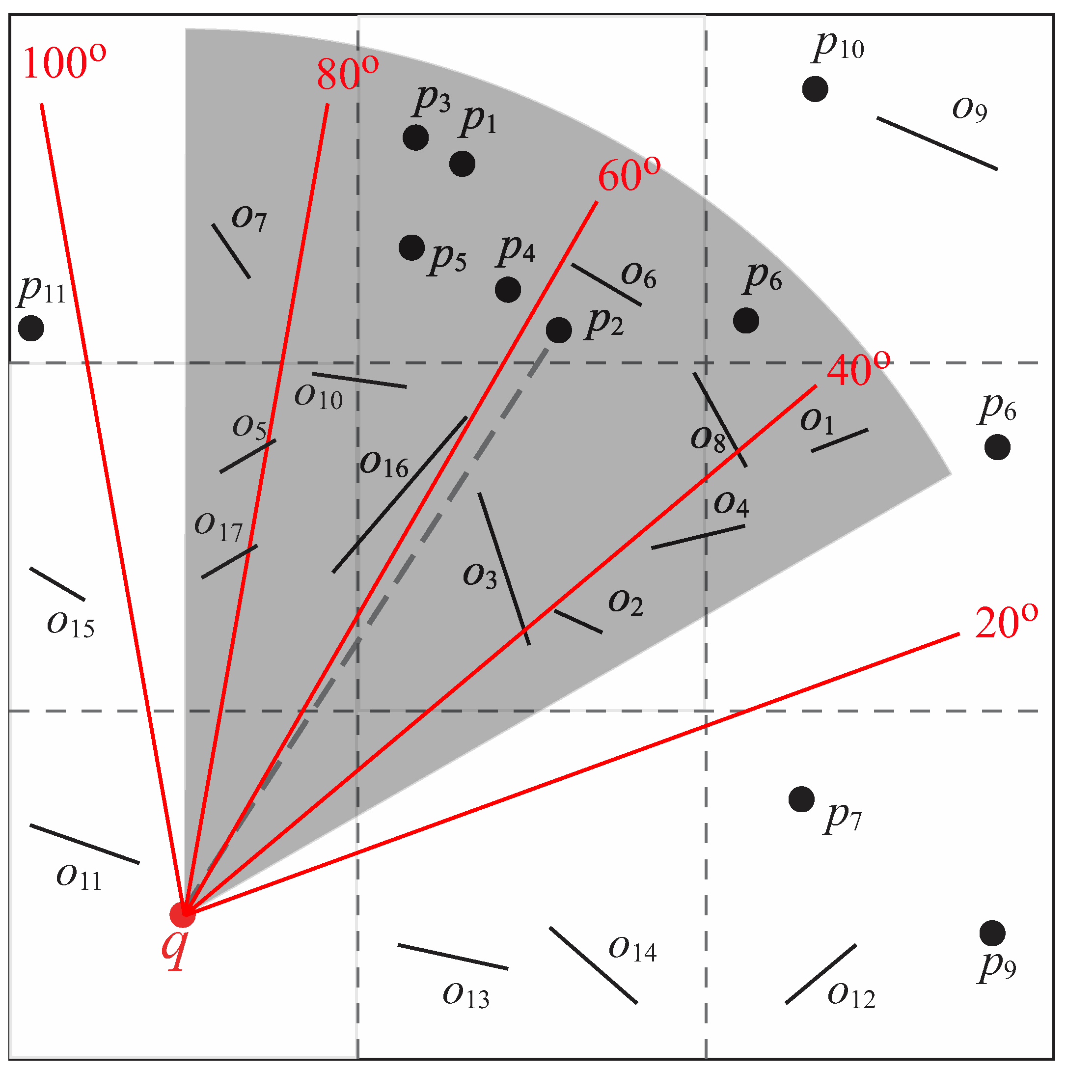
Figure 10 illustrates an example of $V2$-$kNN(q)$ with $q(l,r,\theta )$, $P=\{p_1,p_2,p_3,p_4,p_5\}$, and $O=\{o_1,o_2\}$. We assume that k = 2. In Figure 10, we can find that the $p_1$, $p_3$, $p_4$, $p_5$ are the candidate data objects that are in the view field of q. Although $p_1$, $p_3$ are the closest objects compared to $p_5$ w.r.t to q, they are not visible to q. Therefore, they are not the solutions to $V2$-$kNN$. The data objects meet all of the requirements in Definition 4 $V2$-$kNN(q)$ = $\{p_4,p_5\}$ ordered by their distance w.r.t q.

3.2. Indexing Scheme

To enhance the query processing performance, we use a grid index to collect data objects and obstacles in the data space. We adopt the grid index as it is known as an efficient method [35] for spatial queries. Figure 11 illustrates an example of our index. We divide the data space using grid cells sized $m\times m$, where m is a system parameter that defines the cell size of the grid. Each cell stores the position information of data objects and obstacles inside it. For example, cell $C_{2,3}$ stores the position information of data object $p_2$ and obstacle $o_2$. Note that, if an obstacle o is located in several cells at the same time (e.g., $o_1$), the position information of the obstacle must be stored in every cell with which it has an intersection. For example, the location information of $o_1$ is stored in $C_{2,2}$ and $C_{3,2}$.

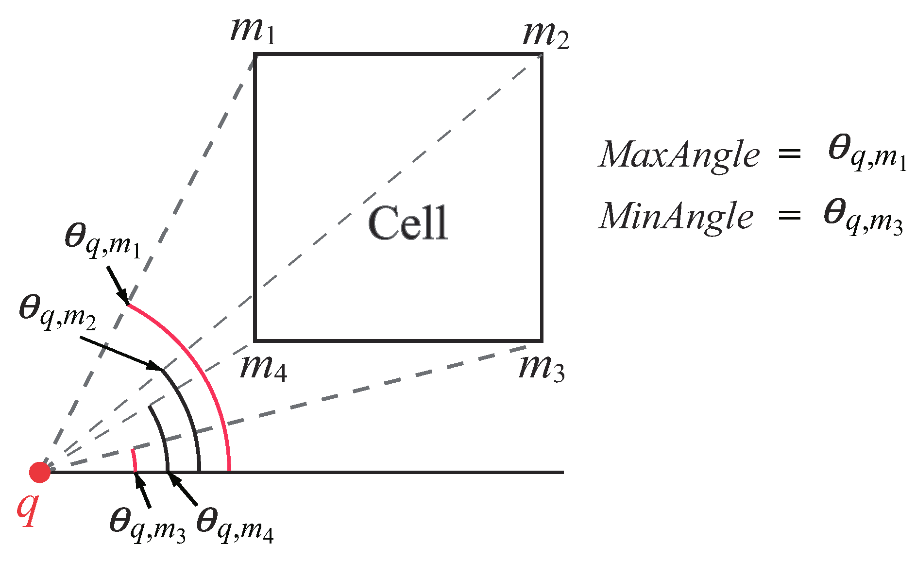
To check whether a view field covers a cell C, we first define the following three terms: $MinDist(q,C)$, $MinAngle$, and $MaxAngle$.

Definition 5.

Minimum distance between a query q and a cell C, $MinDist(q,C)$

If query q is inside the cell, then $MinDist(q,C)$ is zero. Otherwise, the $MinDist(q,C)$ is the Euclidean distance between q and the closest edge of C.

Definition 6.

$MinAngle$ and $MaxAngle$ [24]

Let $\{m1,m2,m3,m4\}$ be the four vertices of a cell C. We use ${\theta }_{q,m_i}(i=1,2,\cdots ,4)$ to denote the angle between $\overline{q{m}_i}$ and the positive x-axis. The min angle and max angle between q and C are defined as follows:

• $MinAngle(q,C)=Min({\theta }_{q,m_1},{\theta }_{q,m_2},{\theta }_{q,m_3},{\theta }_{q,m_4})$.
• $MaxAngle(q,C)=Max({\theta }_{q,m_1},{\theta }_{q,m_2},{\theta }_{q,m_3},{\theta }_{q,m_4})$.

Figure 12 shows an example of $MinAngle(q,C)$ and $MaxAngle(q,C)$.

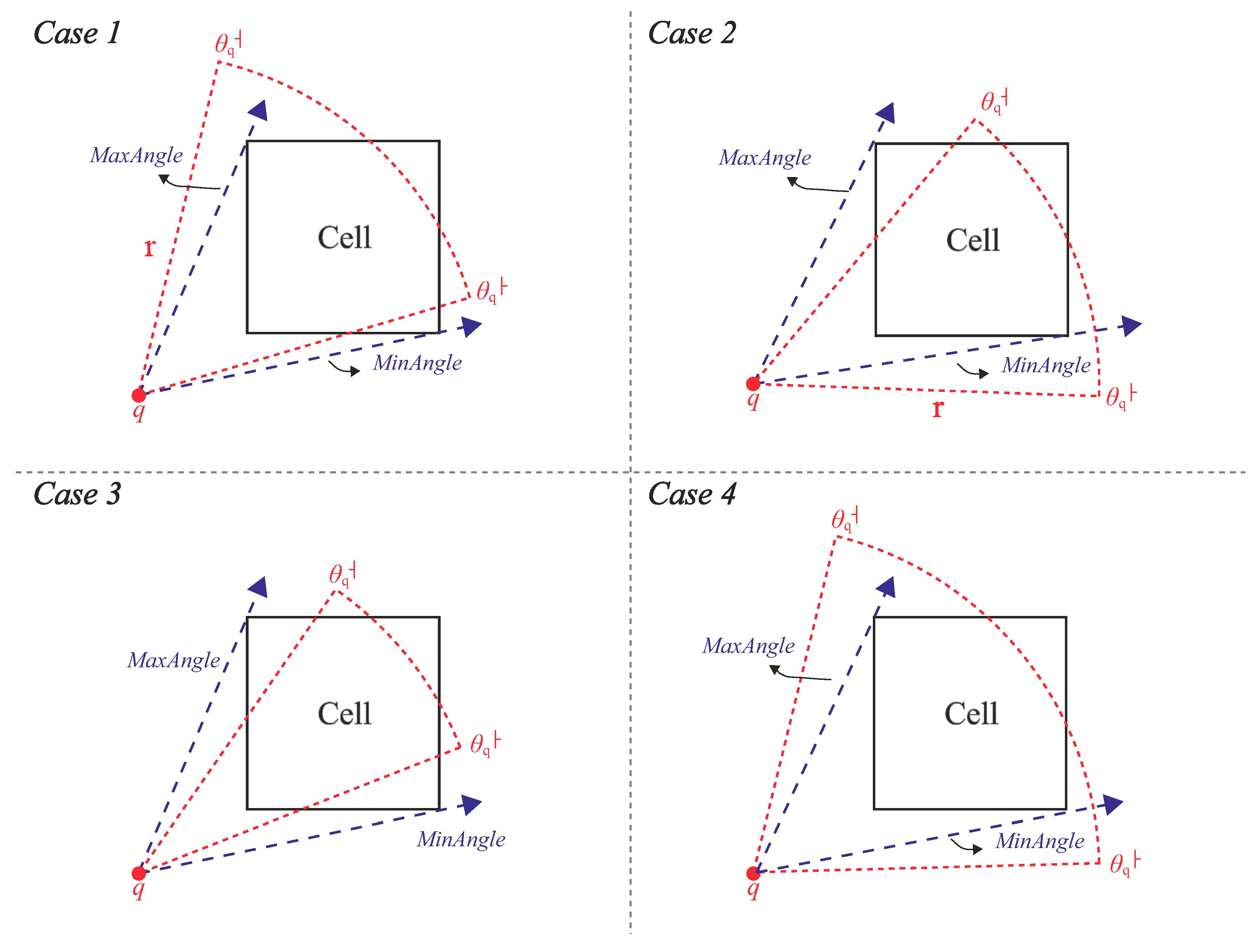
Given a query $q(l,r,\theta )$ and a grid cell C, if q’s view field covers C, then (1) the minimum distance between q and C must be less than or equal to r (i.e., $MinDist(q,C)\le r$) and (2) the relationship among ${\theta }_q^{⊢},{\theta }_q^{⊣}$, $MinAngle(q,C)$ and $MaxAngle(q,C)$ must satisfy one of the following four cases [24]:

• $MinAngle$≤${\theta }_q^{⊢}$≤$MaxAngle$, and $MaxAngle$≤${\theta }_q^{⊣}$ (see Case 1 in Figure 13)
• ${\theta }_q^{⊢}$≤$MinAngle$, and $MinAngle$≤${\theta }_q^{⊣}$≤$MaxAngle$ (see Case 2 in Figure 13)
• $MinAngle$≤${\theta }_q^{⊢}$≤$MaxAngle$, and $MinAngle$≤${\theta }_q^{⊣}$≤$MaxAngle$ (see Case 3 in Figure 13)
• ${\theta }_q^{⊢}$≤$MinAngle$, and $MaxAngle$≤${\theta }_q^{⊣}$ (see Case 4 in Figure 13)

4. V2-kNN Query Processing

4.1. The Baseline Algorithm

Given a V2-kNN query $q(l,r,\theta )$, a set of data objects P, and a set of obstacles O, we assume P and O are indexed by the grid index proposed in Section 3.2. The intuitive approach to process q is to access all the cells covered by q’s view field. Then, we retrieve all the data objects and obstacles in the covering cells. Finally, we check the visibility of all the retrieved data objects and return the k visible nearest data objects to the user as the answer.

Our first algorithm, the baseline algorithm, is designed based on the aforementioned idea. The baseline algorithm is extended from the Fan-shaped Exploration $(FE)$ algorithm [24], which is the most well-known and efficient algorithm that can retrieve nearest data objects in a view field. The difference between ours and the FE algorithm is that the FE algorithm does not consider the obstacles that exist in many real-life scenarios.

The overall procedure of the baseline algorithm is presented in Algorithm 1. The baseline algorithm first initializes two empty min-heaps H and $RL$, as well as an empty set $OL$. H sorts accessed cells according to their minimum possible distance to q (see Definition 5); $RL$ maintains candidate data objects that may eventually become query results; and $OL$ retains already accessed obstacles. The variable $best\_dist$ is defined as the visible distance of the kth visible data object of q, and it is set to ∞ at the beginning of the algorithm. Initially, the algorithm pushes the cells containing q into H (Lines 5–6). Each time, the algorithm pops out the top element of H and puts it in a variable $C_{cur}$ (i.e., the current cell). Then, the baseline algorithm calls the VC algorithm (Visibility Check algorithm; see Algorithm 2) to check the visibility of data objects residing in $C_{cur}$. After that, the CAC algorithm (Check Adjacent Cells algorithm; see Algorithm 3) is called to insert four adjacent cells of $C_{cur}$ into H.

Algorithm 1. The baseline algorithm.

The VC algorithm (see Algorithm 2) first puts all the obstacles in $C_{cur}$ into set $OL$ (Lines 1–2). Then, it examines the visibility of each data object p in $C_{cur}$ (Lines 4–9). If p is invisible to q, then we discard it. Otherwise, the VC algorithm pushes p into $RL$ as it may become the final result (Line 11). In addition, the VC algorithm updates $best\_dist$ if there are more than k elements in $RL$ (Line 12).

Algorithm 2. Visibility Check (VC) algorithm.

Algorithm 3. Check Adjacent Cells (CAC) algorithm.

Given a current cell $C_{cur}$, the CAC algorithm inserts each of $C_{cur}$’s adjacent cells C into H if C satisfies the following conditions: (1) C is a non-visited cell (Line 2); (2) C overlaps with q’s view field (Line 3); and (3) the minimum possible distance between q and C is less than or equal to $best\_dist$ (line 4). Condition (3) indicates that the cell C may contain data objects with a distance smaller than $best\_dist$. Thus, we should keep it for further examination.

The baseline algorithm terminates in two cases. Case 1: Heap H is empty (Line 7 of Algorithm 1). This means that the baseline algorithm has explored all the cells that overlap with the view field. Case 2: The current cell $C_{cur}$ has $MinDist(q,C_{cur})>best\_dist$ (Line 9 of Algorithm 1); that is, all the data objects contained in the remaining cells in H whose distances to q are larger than $best\_dist$. Therefore, they cannot become part of the final result.

We use Figure 14 to explain how the baseline algorithm works. In this example, k is two.

Table 2. The example steps of the baseline algorithm.

Round	Visited Cell	Heap H	Obstacles to Be Checked	Visited Data Object(s)	$\mathit{RL}$	$\mathit{best}\_\mathit{dist}$
1	$C_{1,2}$	$C_{2,2},C_{1,3}$	$o_1$	$p_7$	$\varphi$	∞
2	$C_{2,2}$	$C_{1,2},C_{2,3},C_{3,2}$	$o_1,o_3,o_4$	$p_3$	$\varphi$	∞
3	$C_{1,3}$	$C_{2,3},C_{3,2},C_{1,4}$	$\varphi$	$\varphi$	$\varphi$	∞
4	$C_{2,3}$	$C_{3,2},C_{1,4},C_{3,3},C_{2,4}$	$o_1,o_3,o_4,o_5,o_6$	$p_5$	$p_5$	∞
5	$C_{3,2}$	$C_{1,4},C_{3,3},C_{2,4},C_{4,2}$	$o_1,o_3,o_4,o_5,o_6$	$p_2$	$p_5$	∞
6	$C_{1,4}$	$C_{3,3},C_{2,4},C_{4,2}$	$o_1,o_3,o_4,o_5,o_6,o_7$	$p_4$	$p_5$	∞
7	$C_{3,3}$	$C_{2,4},C_{3,4},C_{4,2},C_{4,3}$	$o_1,o_2,o_3,o_4,o_5,o_6,o_7$	$p_1$	$p_5$	∞
8	$C_{2,4}$	$C_{3,4},C_{4,2},C_{4,3}$	$o_1,o_2,o_3,o_4,o_5,o_6,o_7$	$p_6$	$p_5,p_6$	$dist(q,p_6)$

shows the content of each data structure when the baseline algorithm is running. We start form the cell in which q is located (i.e., $C_{1,2}$). First, we call the VC algorithm (i.e., Algorithm 2) to check the visibility of data objects in $C_{1,2}$. The VC algorithm first puts obstacle $o_1$ into $OL$ as it falls in the view field. Then, the VC algorithm checks the visibility of $p_7$ by comparing $p_7$ with all the obstacles in $OL$. $p_7$ is discard as it is blocked by $o_1$. After that, we call the CAC algorithm (i.e., Algorithm 3) to check $C_{1,2}$’s neighboring (i.e., above, below, left, right) cells to see if they overlap the view field of q. The CAC algorithm puts these overlapping cells (i.e., $C_{2,2}$ and $C_{1,3}$) into heap H. The second row of Table 2 shows the content of each data structure after visiting $C_{1,2}$. Note that although $C_{1,1}$ and $C_{0,2}$ are the adjacent cells of $C_{1,2}$, they are not put into H as they are outside the view field.

Then, we repeat the previous procedures to visit $C_{2,2}$ and $C_{1,3}$. When visiting $C_{2,3}$, we find the first visible data object $p_5$ and insert it into $RL$. The $best\_dist$ is still ∞ as $k=2$, and we only find one candidate. Again, we repeat the same procedure to visit cells $C_{3,2}$, $C_{1,4}$, $C_{3,3}$, and $C_{2,4}$. After visiting $C_{2,4}$, we find the second visible data object $p_6$. We update $best\_dist$ as $dist(q,p_6)$. At this time, we find that the top element of H is $C_{3,4}$, and we observe that $MinDist(q,C_{3,4})>best\_dist=dist(q,p_6)$. This means that distances of all the unseen data objects (i.e., $p_9$ and $p_{12}$ in Figure 14) to q are larger than $dist(q,p_6)$. Therefore, we can terminate the baseline algorithm.

4.2. The Influential Cells Algorithm

The baseline algorithm is simple in design and easy to implement. The main drawback of the baseline algorithm is that it requires the comparison between a data object p and all accessed obstacles when performing the visibility check. We take $p_6$ in Figure 14 as an example. To check whether $p_6$ is visible to q, the baseline algorithm lets $p_6$ be examined with seven obstacles (i.e., $o_1$, $o_2$, $o_3$, $o_4$, $o_5$, $o_6$, $o_7$). However, we find that the cells $C_{2,2}$ and $C_{3,3}$ have no intersection with the line segment $\overline{p_{6}q}$. This means that all of the obstacles located in cells $C_{2,2}$ and $C_{3,3}$ (i.e., $o_2,o_3$, and $o_4$), have no influence on the visibility of $p_6$. Thus, it is unnecessary to examine $p_6$ with $o_2,o_3$ and $o_4$ when performing the visibility check.

Base on this observation, we design a new algorithm, named the influential cells algorithm, which can improve the performance of the baseline algorithm by reducing the number of obstacles to be checked when checking the visibility of a data object. Before we explain the design of the algorithm, we first introduce the notation of the influential cells.

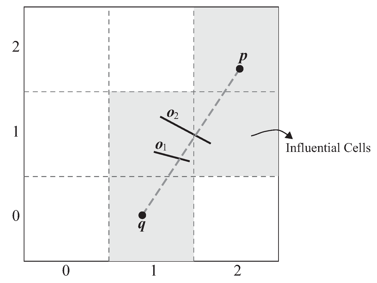
Definition 7.

Influential cells

Given a query $q(l,r,\theta )$ and a data object $p_i$, the influential cells of $p_i$ (denoted as $IC(p_i)$) represent a set of cells that intersect with the line segment $\overline{p_{i}q}$. That is, $IC(p_i)\cap \overline{p_{i}q}\ne \varphi$.

In Figure 15, given a data object p and a query q, the influential cells of p (i.e., $IC(p)$) are cells $C_{1,0},C_{1,1},C_{2,1}$, and $C_{2,2}$, which are highlighted in gray.

Theorem 1 tells us that we can improve the performance of the visibility check by ignoring those obstacles that are not inside the influential cells of a data object.

Theorem 1.

Given a query $q(l,r,\theta )$, a data object p, and a set of obstacles O, let $o\in O$ be an obstacle that is not located in the influential cells of p (i.e., $IC(p)$), then it is impossible for o to affect the visibility of p.

Proof. (By contradiction)

Assume that o makes p invisible to q and p is not located in $IC(p)$. Then, o must intersect with the line segment $\overline{qp}$. Let o intersect with $\overline{qp}$ on a point x. We know that x must lie on the line segment $\overline{qp}$. Thus, x is located in at least one of the influential cells of p, which contradicts the assumption that p is not located in $IC(p)$. □

We extend the visibility check algorithm (i.e., Algorithm 2) to use Theorem 1 to enhance the performance. The pseudocode of the extended version is shown as follows Algorithm 4.

Algorithm 4. Visibility Check Ver. 2 (VC2) algorithm (visibility check algorithm based on Theorem 1).

To find the influential cells of a given data object p, Algorithm 5 checks each cell C in $VCL$ to determine if C intersects with $\overline{pq}$ (Lines 3–4). Note that $VCL$ is a list containing cells that are visited by Algorithm 1.

Algorithm 5. Find Influential Cells (FindIC) algorithm.

We use the same example in Figure 14 to show the process of Algorithm 4 (i.e., the VC2 algorithm). The result is shown in

Table 3. The example steps of the baseline algorithm when calling the Visibility Check Ver. 2 (VC2) algorithm for visibility checking. Note that the “underlined” obstacles are checked in the VC algorithm but are not verified in the VC2 algorithm.

Round	Visited Cell	Heap H	Obstacles to Be Checked	Visited Data Object(s)	$\mathit{RL}$	$\mathit{best}\_\mathit{dist}$
1	$C_{1,2}$	$C_{2,2},C_{1,3}$	$o_1$	$p_7$	$\varphi$	∞
2	$C_{2,2}$	$C_{1,2},C_{2,3},C_{3,2}$	$o_1,o_3,o_4$	$p_3$	$\varphi$	∞
3	$C_{1,3}$	$C_{2,3},C_{3,2},C_{1,4}$	$\varphi$	$\varphi$	$\varphi$	∞
4	$C_{2,3}$	$C_{3,2},C_{1,4},C_{3,3},C_{2,4}$	$o_1,o_3,o_4,o_6,\underline{o_5}$	$p_5$	$p_5$	∞
5	$C_{3,2}$	$C_{1,4},C_{3,3},C_{2,4},C_{4,2}$	$o_1,o_3,o_4,\underline{o_5,o_6}$	$p_2$	$p_5$	∞
6	$C_{1,4}$	$C_{3,3},C_{2,4},C_{4,2}$	$o_1,o_5,o_7,\underline{o_3,o_4,o_6}$	$p_4$	$p_5$	∞
7	$C_{3,3}$	$C_{2,4},C_{3,4},C_{4,2},C_{4,3}$	$o_1,o_2,o_3,o_4,o_6,\underline{o_5,o_7}$	$p_1$	$p_5$	∞
8	$C_{2,4}$	$C_{3,4},C_{4,2},C_{4,3}$	$o_1,o_5,o_6,\underline{o_2,o_3,o_4,o_7}$	$p_6$	$p_5,p_6$	$dist(q,p_6)$

. The forth column illustrates the number of obstacles verified by the VC2 algorithm. Note that the underlined obstacles are ignored by the VC2 algorithm. For example, when checking the visibility of $p_4$ (see the seventh row), the VC algorithm examines six obstacles, while the VC2 algorithm only tests three obstacles. From the above example, we find that the idea of the influential cells reduces the number of obstacles, which are necessary to be checked, thus improving the efficiency of queries. Furthermore, as the view field becomes larger, the number of obstacles inside the view field also increases, leading to a higher computational cost for the visibility check. The idea of the influential cells can identify unqualified obstacles, which improves the performance of the search algorithm even when the view fields are large.

4.3. Direction Index

The idea of the influential cells can greatly reduce the number of obstacles to be checked by the baseline algorithm and thus enhance the search performance. However, there is room to further speedup the search performance. In this subsection, we will introduce the Direction Index ($DI$) method, which builds an index to index the obstacles. When performing the visibility check, the DI method uses the index to further exclude the obstacles that cannot affect the visibility of the data object even if the obstacles are inside the influential cells. We first use an example to illustrate the concept of the direction index.

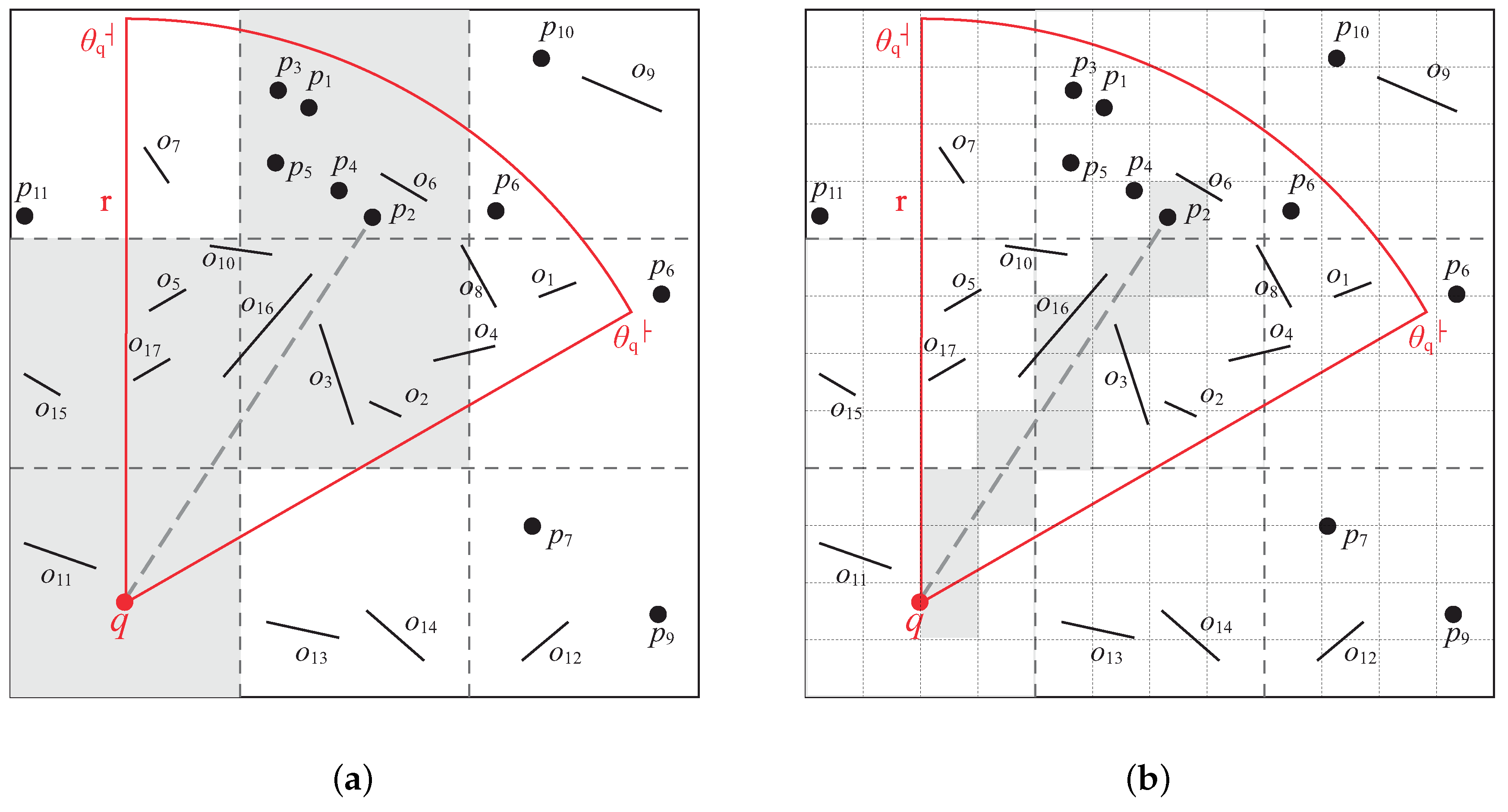
When checking the visibility of $p_2$, in Figure 16a, the IC technique needs to examine nine obstacles (i.e., $o_2$, $o_3$, $o_4$, $o_5$, $o_6$, $o_8$, $o_{10}$, $o_{16}$, and $o_{17}$). However, we find that $o_5$, $o_2$, $o_4$, $o_8$, $o_{10}$, and $o_{17}$ have no influence on the visibility of $p_2$ as they are “far from” the line segment $\overline{p_{2}q}$. The search performance can be improved if we can exclude these obstacles from the visibility test. A question here is how can we identify those obstacles that are far from the line segment?

One solution is to adjust the size of the grid cell. Figure 16b illustrates a fine granularity grid. Compared with Figure 16a, we only need to check three obstacles (i.e., $o_3,o_6$ and $o_{16}$). However, the fine granularity reduces the number of checked obstacles, and it also leads to low search performance as the algorithm needs to access more grid cells. In addition, a fine granularity may make more obstacles be located in several cells at the same time. This means that there would be more repetitive obstacle data stored in each cell. The algorithm must increase the effort to retrieve and filter the repetitive obstacle data. Therefore, it is obvious that adjusting the size of the grid cell still cannot improve the efficiency of the overall execution effectively.

Another solution is to take the “direction of the obstacle” into consideration. More specifically, when checking the visibility of data objects, we can retrieve the obstacles that may influence the visibility of the data object based on therelative anglebetween query point and the obstacles. Based on this idea, we propose the Direction Index (DI) method.

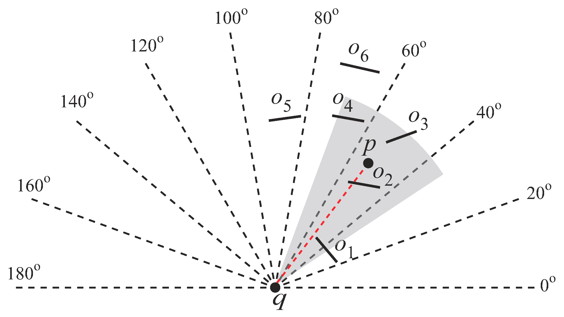
4.3.1. The Design Rationale of the Direction Index

The main idea of the direction index is as follows. Given a splitting angle ${\theta }_{\mathcal{S}}$ (which is a system parameter), we can split the 2D space into $\lceil \frac{{360}^{\circ }}{{\theta }_{\mathcal{S}}}\rceil$ sections equally based on q. The ids of the sections are numbered $0,1,\cdots ,\lceil \frac{{360}^{\circ }}{{\theta }_{\mathcal{S}}}\rceil$− 1. The ith section, $Sectio{n}_i$, represents the angle range $[i\times {\theta }_{\mathcal{S}},(i+1)\times {\theta }_{\mathcal{S}})$. In Figure 17, ${\theta }_{\mathcal{S}}$ is ${20}^{\circ }$, and the 2D space is split into $\frac{{360}^{\circ }}{{20}^{\circ }}=18$ sections. $Sectio{n}_0$ represents $[0^{\circ },{20}^{\circ })$; $Sectio{n}_1$ represents $[{20}^{\circ },{40}^{\circ })$, ⋯, and so on.

From Figure 17, we observe that all the obstacles that are not located in the section where p resides cannot affect the visibility of p. For example, $o_4$ and $o_5$ cannot influence the visibility of p as they do not reside in $Sectio{n}_2$ (i.e., the section where p resides). The observation can be validated by the following theorem.

Theorem 2.

Let p and o be a data object and an obstacle, respectively. p is located in $Sectio{n}_i$, and o resides in $Sectio{n}_j$, where $i\ne j$. o cannot affect the visibility of p.

Proof. 

The proof is omitted as it is trivial. □

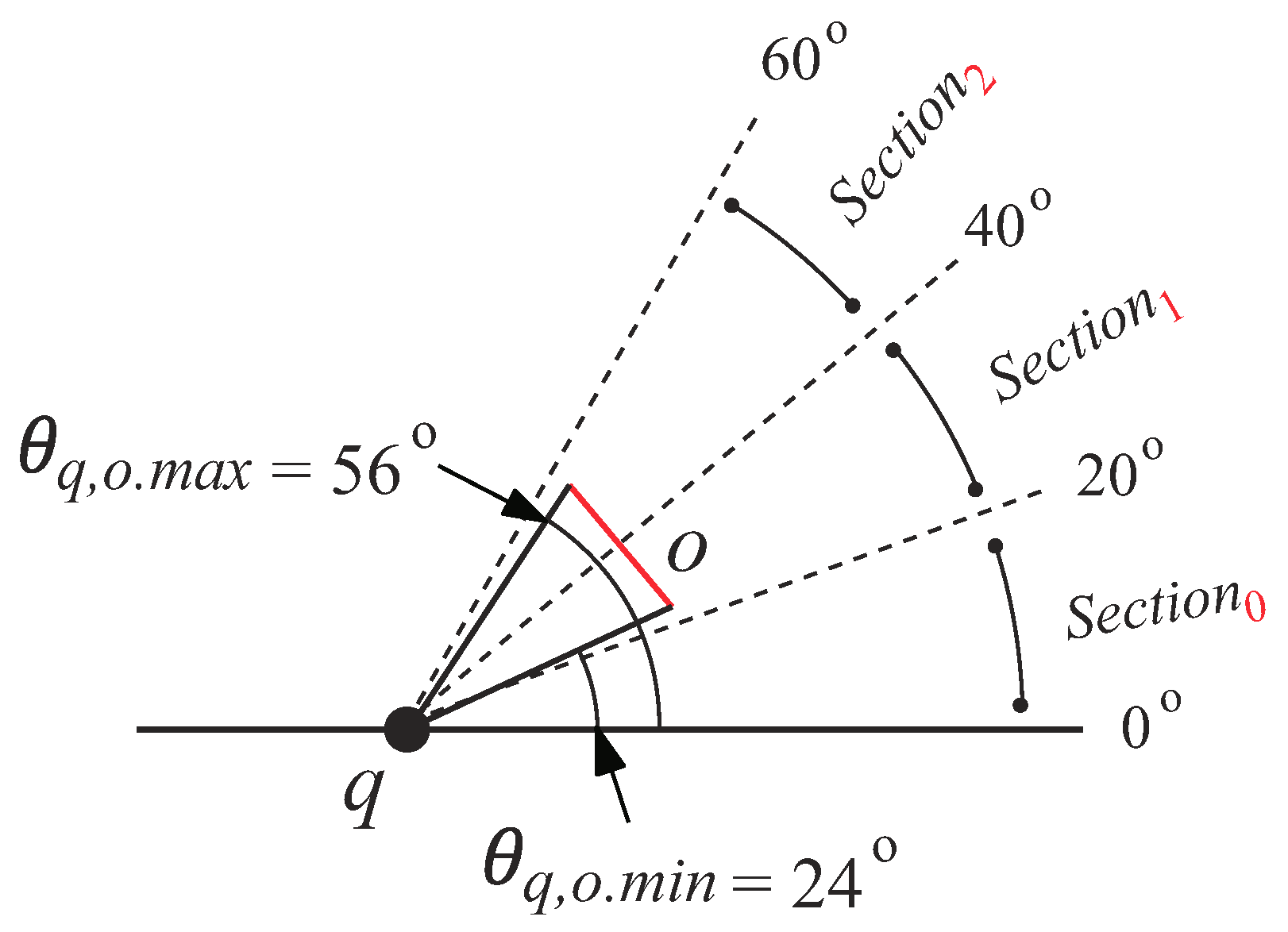
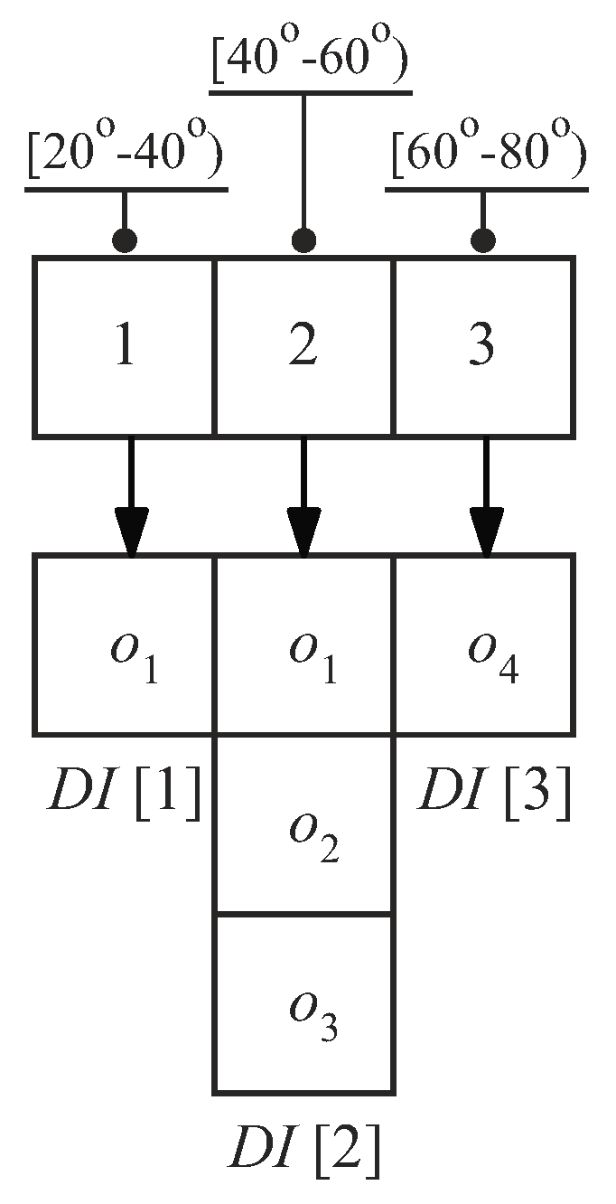
Given an obstacle o and a query point q, we can derive the sections where o is located by using ${\theta }_{q,o.min}$ and ${\theta }_{q,o.max}$; that is, the sections where o is located ranging from $Sectio{n}_{\lfloor \frac{{\theta }_{q,o.min}}{{\theta }_{\mathcal{S}}}\rfloor }$ to $Sectio{n}_{\lfloor \frac{{\theta }_{q,o.max}}{{\theta }_{\mathcal{S}}}\rfloor }$. We take Figure 18 as an example. $\lfloor \frac{{\theta }_{q,o.min}}{{\theta }_{\mathcal{S}}}\rfloor =\lfloor \frac{{24}^{\circ }}{{20}^{\circ }}\rfloor =1$ and $\lfloor \frac{{\theta }_{q,o.min}}{{\theta }_{\mathcal{S}}}\rfloor =\lfloor \frac{{56}^{\circ }}{{20}^{\circ }}\rfloor =2$. Thus, o resides in $Sectio{n}_1$ and $Sectio{n}_2$.

We use a hash table to record the obstacle information in every section. The hash table is named the Direction Index ($DI$). The section id is used as a hash key, and $DI\left[id\right]$ represents a hash value. $DI\left[id\right]$ is a queue that stores the obstacles (1) residing in $Sectio{n}_{id}$ and (2) located in the view field. The queue is sorted in ascending order based on the obstacle’s minimum distance (see Section 3.1) to the query point. Figure 19 shows the content of the $DI$ for Figure 17. Note that only the obstacles residing in $Sectio{n}_1,Sectio{n}_2,$ and $Sectio{n}_3$ are kept in $DI$ as q’s view field overlaps with the three sections. Also note that since $o_1$ falls in $Sectio{n}_1$ and $Sectio{n}_2$, we store $o_1$ in $DI\left[1\right]$, as well as $DI\left[2\right]$.

4.3.2. Using $DI$ for Query Processing

We construct the direction index on-the-fly when processing a query q. Each time the Baseline algorithm visits a cell C, we retrieve the obstacles in C and insert them into a direction index $DI$ (Line 3 in Algorithm 6). To check the visibility of a data object p, we first calculate the section id of the section where p resides (Line 6). Assume that the section id is $id$, then we compare p with all the obstacles in $DI\left[id\right]$. Note that the obstacle in $DI\left[id\right]$ with $MinDist(q,o)$ is greater than $dist(q,p)$, which are discard as they cannot affect the visibility of p (Line 12). Thus, we can safely exclude them and save computational cost.

Algorithm 7 shows the details of inserting an obstacle into the direction index. Lines 1–2 calculate the section id(s). Then, we simply insert the obstacle into the corresponding slots of $DI$.

We use Figure 20 as an example to explain how the direction index works. In the example, k is one, ${\theta }_{\mathcal{S}}$ is ${20}^{\circ }$, and the gray area is the view field. Since $p_2$ falls in $Sectio{n}_2$, we compare $p_2$ with all the obstacles in $Sectio{n}_2$ (i.e., $DI\left[2\right]$) to check its visibility. The obstacles in $DI\left[2\right]$ are $(o_3,o_8,o_6)$ (sorted according to the $MinDist$). We find that $p_2$ is a visible nearest neighbor of q as $o_3$ and $o_8$ cannot block it. Note that the checking process is terminated when we meet $o_6$ as $MinDist(q,o_6)$ is greater than $dist(q,p_2)$, and all the unchecked obstacles ordered after $o_6$ cannot affect $p_2$’s visibility.

In summary, the direction index can reduce unnecessary examinations of obstacles with a smaller value of ${\theta }_{\mathcal{S}}$, as it finds a more precise section, which may influence the visibility of data objects. However, a smaller ${\theta }_{\mathcal{S}}$ means that more obstacles might be located in the different sections at the same time, increasing the storage overhead of the direction index. In the experiment section, we will find the suitable ${\theta }_{\mathcal{S}}$ through simulations.

Algorithm 6. Visibility Check ver. 3 (VC3) algorithm (visibility check algorithm based on Theorem 1).

Algorithm 7. Insert an obstacle into a direction index (InsertToDI) algorithm.

GIVEN: The obstacle o, the direction index $DI$, and the splitting angle ${\theta }_{\mathcal{S}}$   FIND: The direction index $DI$ 1 $start\leftarrow \lfloor \frac{{\theta }_{q,o.min}}{{\theta }_{\mathcal{S}}}\rfloor$; 2 $end\leftarrow \lfloor \frac{{\theta }_{q,o.max}}{{\theta }_{\mathcal{S}}}\rfloor$; 3 for $i\leftarrow start$ to $end$ do Push o into $DI\left[i\right]$;$\phantom{(}$ 4 return $DI$;

4.4. The Invisible Regions Lookup Buffer

4.4.1. Motivation

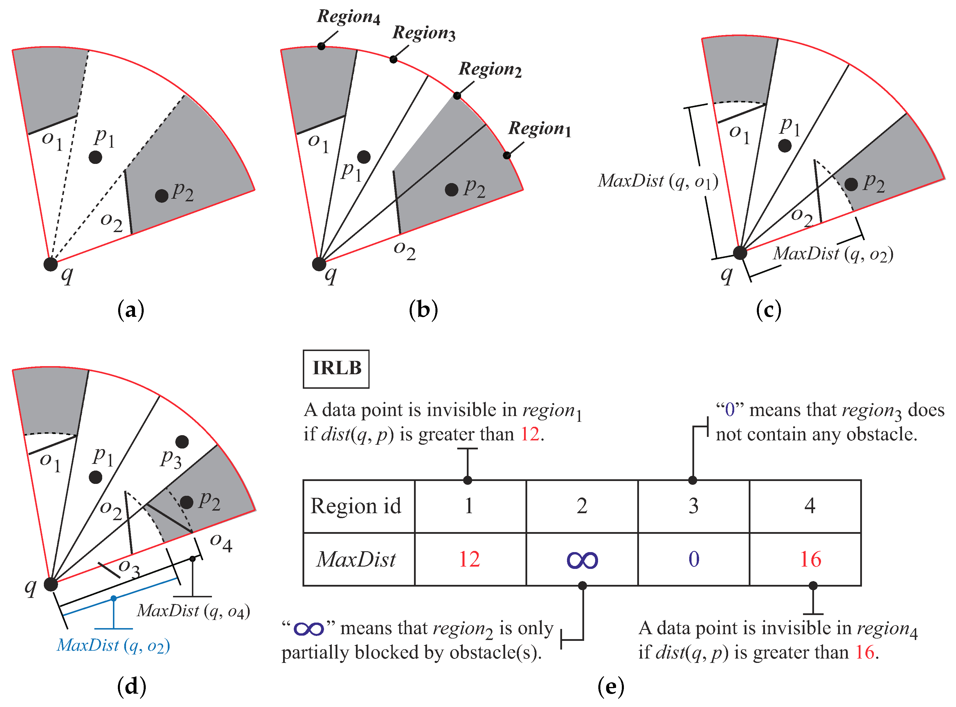
The DI method finds a more precise region that contains visible influential obstacles, improving the efficiency of the visibility check. However, there is still room for further improvement. We use the following example to explain it. In Figure 20, $p_5$ is blocked by $o_{10}$. However, to check its visibility, the $DI$ method not only compares $p_5$ with $o_{10}$, but also examines $p_5$ with $o_5$, $o_{16}$, and $o_{17}$. The same thing happens in the visibility checking of $p_1$ and $p_3$. Obviously, the more obstacles we compare with, the higher processing time the visibility check algorithm consumes. Thus, if we can reduce the number of data-obstacle comparisons, then we can speed-up the process of V2-kNN queries.

To achieve this goal, we propose an effective and light-weight data structure named Invisible Regions Lookup Buffer $(IRLB)$. The idea of $IRLB$ is to keep the “invisible regions” in a hash table. An invisible region is an area blocked by an obstacle. If p falls in o’s invisible region, then p is blocked by o and is invisible to q. Figure 21a shows a view field and the invisible regions (i.e., the gray areas) made by the two obstacles $o_1$ and $o_2$. Since $p_2$ resides in $o_2$’s invisible region, $p_2$ is an invisible data object.

When checking the visibility of a data object p, instead of comparing p with all the obstacles in the same section, we first lookup $IRLB$ to examine if p is inside an invisible region. If yes, p is immediately discarded. Since the underlying data structure of $IRLB$ is a hash table, the checking procedure is very fast (i.e., $O(1)$). Thus, we improve the performance of the V2-kNN search.

The challenge in designing $IRLB$ is that invisible regions are irregular shapes. The construction and storage costs of invisible regions are very high. In addition, testing if a data object is inside an invisible region is also time-consuming since we have to perform many geometric evaluations. To address this problem, we sacrifice the accuracy of invisible regions for faster computation. Our design rationale contains two strategies. We use the following figures to explain them.

First, we divide the view field into several small regions as Figure 21b shows. The advantage of the strategy is that we can classify the relationships between an obstacle and a region into three categories: (1) the region being “fully blocked” by obstacles (e.g., $Regio{n}_1$ and $Regio{n}_4$); (2) the region that is “partially blocked” by obstacles (e.g., $Regio{n}_2$); and (3) the region that does not contain any obstacle (e.g., $Regio{n}_3$).

The second strategy is to use the maximum distance between an obstacle o and the query q (i.e., $MaxDist(q,o)$) to represent the invisible region made by o. The benefits of the strategy are two-fold. First, it reduces the storage cost of each invisible region. The reason is that for each invisible region, we only need to keep a float point variable (i.e., $MaxDist(q,o)$) in the main memory. Second, the invisible region becomes a “regular” pie shape. For example, in Figure 21c, the invisible region made by $o_2$ in $Regio{n}_1$ becomes a regular pie shape. Thus, checking if a data object falling in an invisible region becomes “a piece of cake” task as we only need to compare $dist(q,p)$ with $MaxDist(q,o)$.

Indeed, these strategies degrade the precision of the invisible regions. For example, the invisible region made by $o_1$ in Figure 21c is smaller than that in Figure 21b. Furthermore, we do not record the invisible region in $Regio{n}_2$ as $o_2$ only partially blocks $Regio{n}_2$. However, the design can greatly enhance the performance of the visibility checking. Let us use Figure 21d to explain it. We have to compare $p_2$ with three obstacles (i.e., $o_2,o_3$, and $o_4$) so as to check the visibility of $p_2$ in DI. On the other hand, by using $IRLB$, we only perform one operation (i.e., test whether $dist(q,p_2)>MaxDist(q,o_2)$) and find that $p_2$ is invisible to q. This shows that our design can reduce the number of data-obstacle comparisons and thus enhance the performance of the visibility check. In the next section, we will introduce the details of $IRLB$.

4.4.2. The Construction of $IRLB$

As we did in $DI$, we use an IRLB slitting Angle${\theta }_{IRLB}$ to split the 2D data space into $\lceil \frac{{360}^{\circ }}{{\theta }_{IRLB}}\rceil$ equal-sized regions. The $i^{\mathrm{th}}$ region $Regio{n}_i$ corresponds to angle range $[i\times {\theta }_{IRLB},(i+1)\times {\theta }_{IRLB})$, where $i=0,1,\cdots ,\lceil \frac{{360}^{\circ }}{{\theta }_{IRLB}}\rceil -1$. Note that ${\theta }_{IRLB}$ is a system parameter, and we set ${\theta }_{IRLB}\ll {\theta }_{\mathcal{S}}$ in practical implementations.

$IRLB$ is a hash table to keep the information of invisible regions in each region. $IRLB$ contains $\lceil \frac{{360}^{\circ }}{{\theta }_{IRLB}}\rceil$ elements. Each element is a key-value pair. A key corresponds to the region id. The value for key i, denoted as $IRLB\left[i\right]$, has three possible values:

• $\mathit{IRLB}\left[\mathit{i}\right]$ is zero if $Regio{n}_i$ does not contain any obstacle. For example, in Figure 21d, $Regio{n}_3$ does not contain any obstacle. Thus, $IRLB\left[3\right]$ is zero.
• If $Regio{n}_i$ is fully blocked by a set of obstacles $\mathcal{F}$, then $IRLB\left[i\right]$ is the minimum value of all the maximum distances between a query point q and each obstacle $o_j\in \mathcal{F}$. That is, $IRLB\left[i\right]=mi{n}_{\forall o_j\in \mathcal{F}}(MaxDist(q,o_j))$. For the formal definition of a full block, please refer to Definition 8. For example, in Figure 21d, $Regio{n}_1$ is fully blocked by $\mathcal{F}=\{o_2,o_4\}$. Thus, $IRLB\left[1\right]=min(MaxDist(q,o_2),MaxDist(q,o_4))$.
• $\mathit{IRLB}\left[\mathit{i}\right]$ is ∞ if $Regio{n}_i$ is only partially blocked (see Definition 9) by some obstacles. In Figure 21d, $IRLB\left[2\right]$ is ∞ since $Regio{n}_2$ is partially blocked by $o_2$.

Definition 8.

(Fully blocked)

Given a query $q(l,r,\theta )$ and a region $Regio{n}_i$ with angle range $[i\times {\theta }_{IRLB},(i+1)\times {\theta }_{IRLB})$, $Regio{n}_i$ is fully blocked by the obstacle o if (1) $MaxDist(q,o)\le r$ and (2) ${\theta }_{q,o.min}\le i\times {\theta }_{IRLB}$ and ${\theta }_{q,o.max}\ge (i+1)\times {\theta }_{IRLB}$.

Definition 9.

(Partially blocked)

A region $Regio{n}_i$ is partially blocked by an obstacle o if neither $Regio{n}_i$ is fully blocked by o nor does $Regio{n}_i$ contain any obstacle.

Algorithm 8 shows the pseudocode for inserting an obstacle into $IRLB$. Note that at the beginning, each element in $IRLB$ is initialized to be zero (i.e., $IRLB\left[i\right]=0$ for $i=0,1,\cdots ,\lceil \frac{{360}^{\circ }}{{\theta }_{IRLB}}\rceil -1$). Given an obstacle o, Lines 1–2 determine the ids of regions that are covered by o. For each region $Regio{n}_i$, if it is fully blocked by o, then we set $IRLB\left[i\right]$ to the minimum value of $MaxDist$ (Lines 4–6). Otherwise, $Regio{n}_i$ is partially blocked by o, and $IRLB\left[i\right]$ is set to be ∞ (Lines 7–8).

Figure 21e shows the IRLB for Figure 21d. Since there are two obstacles (i.e., $o_2$ and $o_4$) fully blocking $Regio{n}_1$, $IRLB\left[1\right]=min(MaxDist(q,o_2),MaxDist(q,o_4))=12$. $IRLB\left[2\right]$ is ∞ as $Regio{n}_2$ is partially blocked by $o_2$. Since $Regio{n}_3$ does not contain any obstacle, $IRLB\left[3\right]$ is zero. There is only one obstacle (i.e., $o_1$) fully blocking $Regio{n}_4$; thus, $IRLB\left[4\right]=MaxDist(q,o_1)=16$.

Algorithm 8. Insert an obstacle into an Invisible Regions Lookup Buffer (InsertToIRLB) algorithm.

4.4.3. DI with $IRLB$

In this section, we present a new V2-kNN search algorithm that leverages the $IRLB$ and the DI method. The algorithm is a two-phase visible kNN search algorithm. In the first phase, we use $IRLB$ to categorize a data object p quickly into one of two types: (1) p is a candidate data object or (2) p is an invisible one. In the second phase, only the candidate data objects are processed by the DI method to find the exact answer. Since $IRLB$ is fast, we can quickly reduce the search space and thus improve the efficiency of the DI method. The pseudocode of our search algorithm is shown in Algorithm 9. Lines 1–4 initialize the data structures $DI$ and $IRLB$. In Phase 1, given a data object p, we first calculate the region in which p is located (Line 7). Then, we use $IRLB$ to determine the visibility of p quickly. We state the decision rules as follows.

• Case 1: $\mathit{IRLB}\left[\mathit{i}\right]$ is zero. This means that p falls in a region that does not contain any obstacle. Thus, p is visible to q (Line 9). For example, $p_1$ in Figure 21d is visible to q.
• Case 2: $\mathit{IRLB}\left[\mathit{i}\right]\le \mathit{dist}(\mathit{q},\mathit{p})$. In this case, p is blocked by at least one obstacle in $Regio{n}_i$. Thus, p is invisible to q and can be directly dropped (Line 10). For example, $p_2$ in $Regio{n}_1$ (Figure 21d) is blocked by $o_2$ and $o_4$. Therefore, $p_2$ is invisible to q.
• Case 3: If p does not belong to the above two cases, then we call DI to check p’s visibility (i.e., Lines 12–17). For the details of DI, please refer to Section 4.3.2. In Figure 21d, we cannot determine the visibility of $p_3$ by using $IRLB$. Thus, we pass $p_3$ to DI for further processing.

Algorithm 9. Visibility Check Ver. 4 (VC4) Algorithm (visibility check algorithm based on DI and $IRLB$).

The correctness of Algorithm 9 is guaranteed by Theorems 3 and 4.

Theorem 3.

Given a data object p inside a region $Regio{n}_i$, p is invisible to q if $IRLB\left[i\right]\ne 0$ and $dist(q,p)\ge IRLB\left[i\right]$. More precisely, if p is blocked by an obstacle o in $Regio{n}_i$, then $Regio{n}_i$ is fully blocked by o and $dist(q,p)\ge MaxDist(q,o)=IRLB\left[i\right]$.

Proof. 

o fully blocks $Regio{n}_i$. Since o is a “continuous” line segment, we can find a point x on o such that ${\theta }_{q,o.min}\le {\theta }_{q,p}={\theta }_{q,x}\le {\theta }_{q,o.max}$. If we can show that x lies on $\overline{qp}$, then we prove that p is invisible to q. Fact 1: The cross product of $\overrightarrow{qp}\times \overrightarrow{qx}=$ $dist(q,p)*dist(q,x)*sin({\theta }_{q,p}-{\theta }_{q,x})=$ $dist(q,p)*dist(q,x)*0=0$. This means that q, x, and p are collinear. Fact 2: Since x lies on line segment o, $dist(q,x)\le MaxDist(q,o)$. Furthermore, we know that $dist(q,p)\ge MaxDist(q,o)$. We have $dist(q,x)\le dist(q,p)$. Thus, x lies between q and p. From Fact 1 and Fact 2, we conclude that x lies on $\overline{qp}$, and thus, p is blocked by o. □

Theorem 4.

If p is inside $Regio{n}_i$ and $Regio{n}_i$ does not contain any obstacle, then p is a visible data object.

Proof. 

We prove it by contradiction. Assume that p is invisible to q. There must be an obstacle o that intersects with line segment $\overline{qp}$ on a point x. Since $\overline{qp}$ falls in $Regio{n}_i$, x also resides in $Regio{n}_i$. Thus, o must be in $Regio{n}_i$. □

4.4.4. Discussion

The effectiveness of $IRLB$ greatly depends on ${\theta }_{IRLB}$. For example, in Figure 21d, if we use a smaller ${\theta }_{IRLB}$ and split the data space with a finer granularity, then $p_3$ would fall in a region that is fully blocked by $o_2$. Therefore, we can directly drop $p_3$ without invoking DI. In our experiment, we used ${\theta }_{IRLB}=1^{\circ }$, and we found that the visibility of over 99% of data objects was identified by $IRLB$. Only 1% of data objects required further processing.

Since the design of $IRLB$ is very simple, its storage overhead is very small. In our simulation, the $IRLB$ with ${\theta }_{IRLB}=1^{\circ }$ required $\frac{{360}^{\circ }}{1^{\circ }}\times 2(floatpointvariables)\times 64(bits)=$ 46,080 bits $\approx 6$ KB. Compared with modern-day computer systems that usually have more than 8 GB main memory capacity, the storage overhead of $IRLB$ is negligible.

5. Experimental Study

In this section, we evaluate and compare the performance of the algorithms we proposed through extensive experiments. We first introduce our experimental environment, varying parameters and the methods of performance evaluation, then giving detailed descriptions and analysis for each experiment.

5.1. Simulation Environments

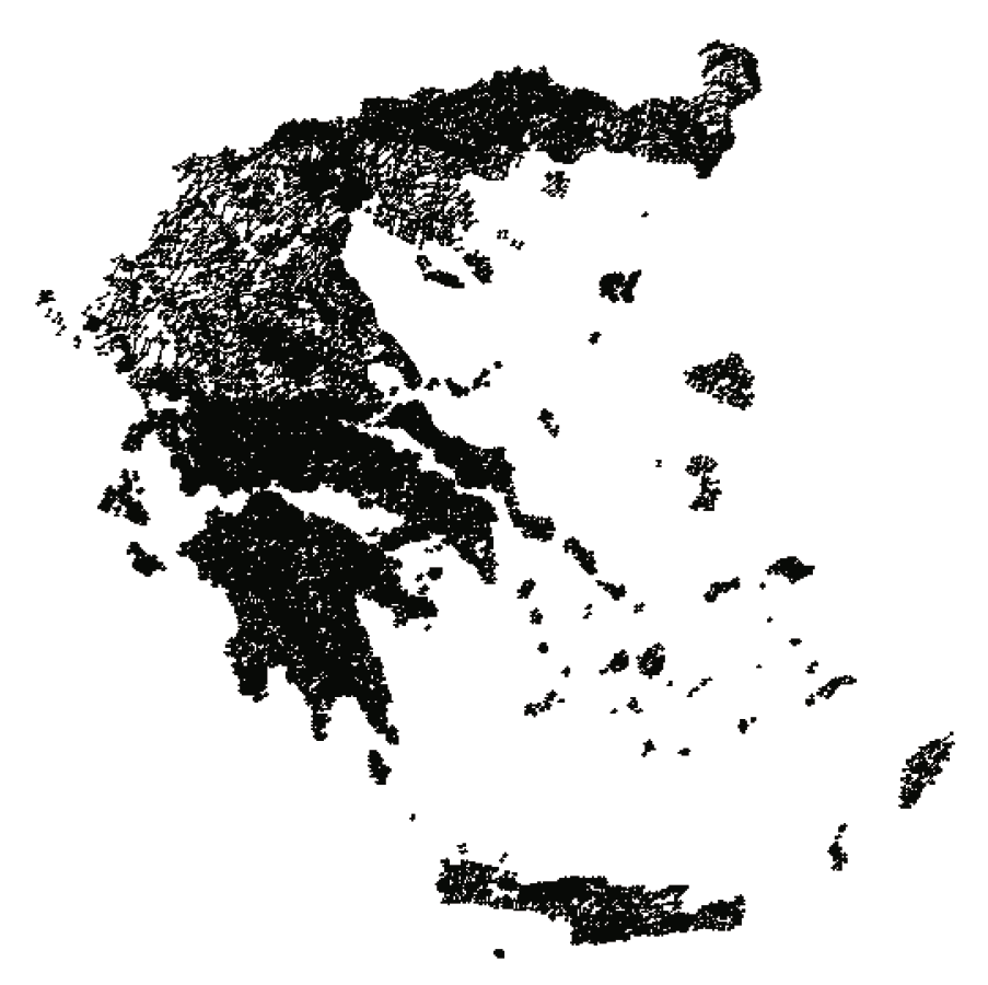
All of the algorithms were implemented in Java, and the experiments were conducted on a Windows 10 desktop computer with Intel(R) Core(TM) i5-4460 CPU 3.20 GHz and 8 GB RAM. Both real and synthetic datasets were used in our experiments. To reflect the real-world situations of our problem with the existence of obstacles, we used a real dataset that is widely used in the research of visible nearest neighbor queries [4,18,20,30], containing 24,650 river distribution information data in Greece [36] as our obstacle sets, and each of them is represented by a bounding rectangle. We took the diagonals of the rectangles as the obstacles in our experiments, and the distribution is shown in Figure 22.

Two types of data objects were generated, the Gaussian and the Zipfian datasets. For the Gaussian dataset, the location of a data object was Gaussian distributed with mean equal to 1000 and variance equal to 2000. For the Zipfian distribution, the data objects were more dense around the center of the data space and became sparse quickly toward the outside. In the following experiments, we used “RG” to represent the simulation being based on the Real obstacle dataset and the Gaussian distributed dataset. Similarly, “RZ” indicates that the simulation was based on the Real obstacle dataset and the Zipfian dataset. In our experiments, the number of data objects was varied from 10 k–1000 k. All of the obstacles and data objects were mapped into a domain of size [0, 20,000] × [0, 20,000] and were indexed in grid cell partitions.

The locations of the query points were also generated by the Gaussian and the Zipfian distributions. When we generated a query point q, we uniformly selected a value from $[0^{\circ },{360}^{\circ }]$ as the starting angle (i.e., ${\theta }_q^{⊢}$, please refer to Section 3.1) of the view field. The view field angle $\theta$ and the maximum visible distance r were uniformly chosen from $[{60}^{\circ },{360}^{\circ }]$ and [1, 10,000], respectively. We ran 100 queries for each experiment, and the average performance is reported.

Table 4. Parameters and values of the experiments.

Parameter	Value Range	Default Value
$\left|P\right|$	10 k–1000 k	100 k
$\left|O\right|$	5000–24,650	24,650
$CellSize$$(m)$	100–2500	1000
k	10–50	20
$\theta$	60–${360}^{\circ }$	${120}^{\circ }$
r	1 half of map	4000
${\theta }_{\mathcal{S}}$	1–${60}^{\circ }$	${10}^{\circ }$
${\theta }_{IRLB}$	1–${60}^{\circ }$	$1^{\circ }$

summarizes the parameters used, where the “Default Value” column shows the default values.

We evaluated four algorithms in the experiments as listed below:

• Baseline: the straightforward method to process V2-kNN queries (see Section 4.1). The baseline algorithm is extended from the Fan-shaped Exploration (FE) algorithm [24]. We can understand the effectiveness of our design by comparing the performance of the EF algorithm and our technique proposed in the paper.
• Influential Cells algorithm (IC algorithm): the V2-kNN query processing method that leverages influential cells to decrease the search space (see Section 4.2).
• Direction Index algorithm (DI algorithm): this algorithm uses the direction index as the index of in-view-field obstacles. It reduces unnecessary obstacles to perform the visibility check and further improves the efficiency of the algorithm, with its direction and distance perspectives (see Section 4.3).
• Invisible Regions Lookup Buffer algorithm (IRLB algorithm): The algorithm uses an efficient data structure (i.e., IRLB) to index the invisible regions in the view field. Then, the algorithm uses IRLB to prune invisible objects in advance, further reducing the computations in the visibility check (see Section 4.4).

We measured the computational cost by recording the query processing time. To show the efficiency of our pruning technique, we also considered the number of accessed obstacles. The lower the number of accessed obstacles, the more effective the pruning method.

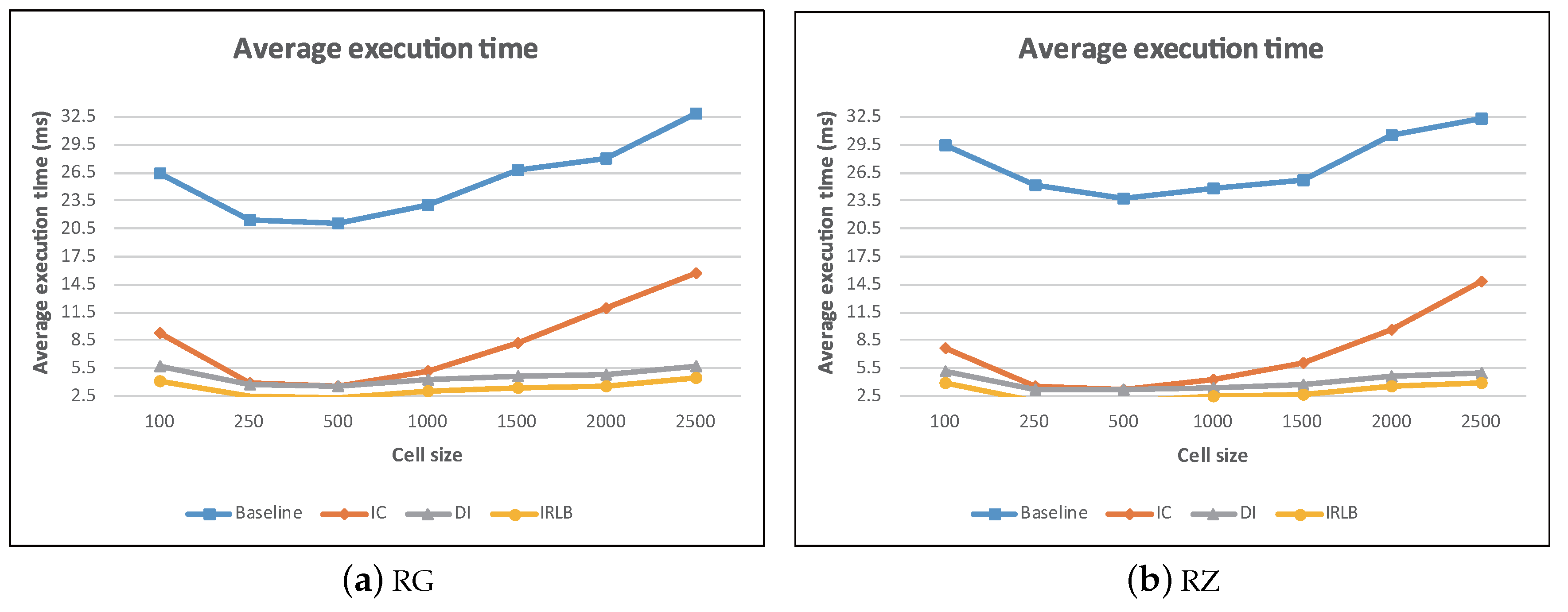
5.2. The Effect of Cell Granularity $(m)$

In this experiment, we evaluated the performance of the proposed algorithms under various cell granularity settings. We varied the cell size m from 100–2500 and record the average execution time of each algorithm in Figure 23a,b. We observed that with a large m value (i.e., large cell size), each cell contained a large number of data objects and obstacles. All algorithms spent much effort to filter out irrelevant data objects and obstacles. This incurred excessive computational cost. On the other hand, with a small m value (i.e., small cell size), each cell contained a small number of data objects and obstacles. Although, this results in lower CPU time, where the visibility check is performed among a few data objects and obstacles. However, the algorithms needed to access more cells so as to find the query result. Thus, additional computational overhead was incurred.

From Figure 23, we also find that IC, DI, and IRLB greatly outperformed the baseline algorithm. This means that our proposed data pruning techniques can efficiently filter out unaffected data objects or obstacles and thus decrease the computational overhead of the visibility check.

Figure 23a,b also shows that the performance of IC was strongly dependent on the cell size. In our experiment, the efficiency of IC decreased substantially when the cell size became larger than 1000. The reason is that the IC algorithm finds influential cells $IC(p)$ when checking the visibility of the data object p. When the cell size becomes larger, each cell contains more obstacles. Therefore, in the larger size cell, IC had to check the visibility with more obstacles, making the efficiency of IC algorithm decrease when the cell size increased over 1000. On the other hand, the pruning techniques of DI and IRLB did not rely heavily on the grid size. Thus, DI and IRLB performed more stably than IC as m increased.

5.3. The Effect of Number of Data Objects ($\left|P\right|$)

In this experiment, we studied the performance of all approaches against the data object cardinalities ($\left|P\right|$: 10 k up to 1000 k). The result is depicted in Figure 24. We notice that all the algorithms incurred a longer execution time with the increase of $\left|P\right|$. This is mainly because the algorithms had to perform more visibility checks as $\left|P\right|$ increased.

Among all the methods, Baseline performed the worst as it had to do exhaustive comparisons between each data object and all obstacles. Meanwhile, IC, DI, and IRLB outperformed baseline as they can avoid many comparisons. Finally, IRLB showed its superiority over others due to the following two reasons. First, the data were pruned efficiently by checking the invisible regions lookup buffer. We can avoid computational overhead for performing the visibility check. Second, IRLB can terminate the search early as soon as visible data objects are identified.

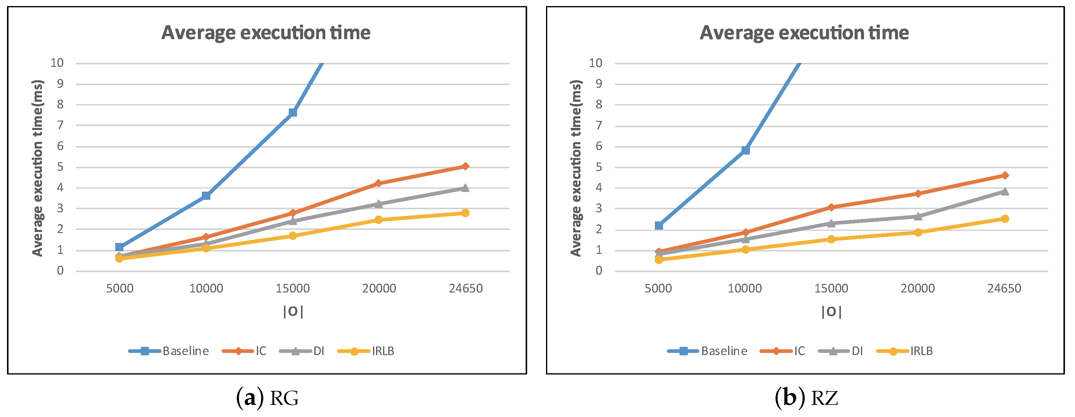
5.4. The Effect of Number of Obstacles $(|O|)$

Figure 25a,b shows the performance results for all algorithms with the increase of the number of obstacles. In this experiment, we varied the number of obstacles $\left|O\right|$ by randomly sampling the 24,650 obstacles from rivers in Greece. Figure 25 shows that the average execution time of all the algorithms increased when $\left|O\right|$ increased. The main reason is that when $\left|O\right|$ increased, the number of in-view-field obstacles may increase as well. Therefore, the examined obstacles of all the algorithms increased while doing visibility checking of in-view-field objects, thus leading to increasing computational cost.

IC, DI, and IRLB performed better than baseline as they use obstacle pruning techniques to reduce the number of obstacles that need to be compared, resulting in effective visibility check. Also note that DI and IRLB outperformed IC. This shows that the direction-based filter can prune more irrelevant obstacles than the cell-based filter. Finally, IRLB leveraged the invisible regions lookup buffer to discard the invisible data objects from further examination, leading to faster query processing.

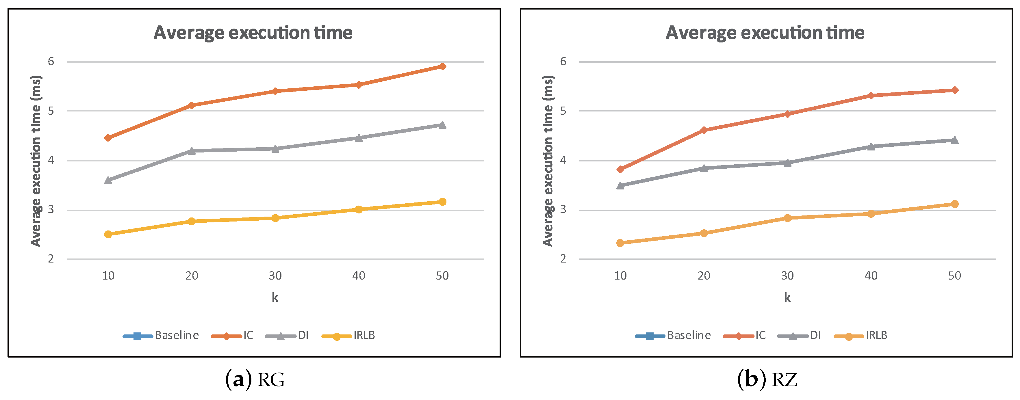
5.5. The Effect of k

This experiment was to study the influence of k for baseline, IC, DI, and IRLB, and the results are plotted in Figure 26a,b. Note that we did not draw the curves of baseline because the average execution time of baseline was too large. The average execution time of baseline is about 4.5-times and eight-times higher than that of IC and IRLB, respectively. As expected, the execution times of all algorithms increased as k grew. However, DI and IRLB remained superior over baseline and IC. While the average execution time of all the algorithms increased linearly as k increased, the rate of increase for DI and IRLB was slower. This is primarily because as k increased, the number of visibility checks also increased. Therefore, the direction-based pruning technique for DI and IRLB can efficiently decrease the number of obstacle comparisons when checking the visibility of a data object, leading to a low search time.

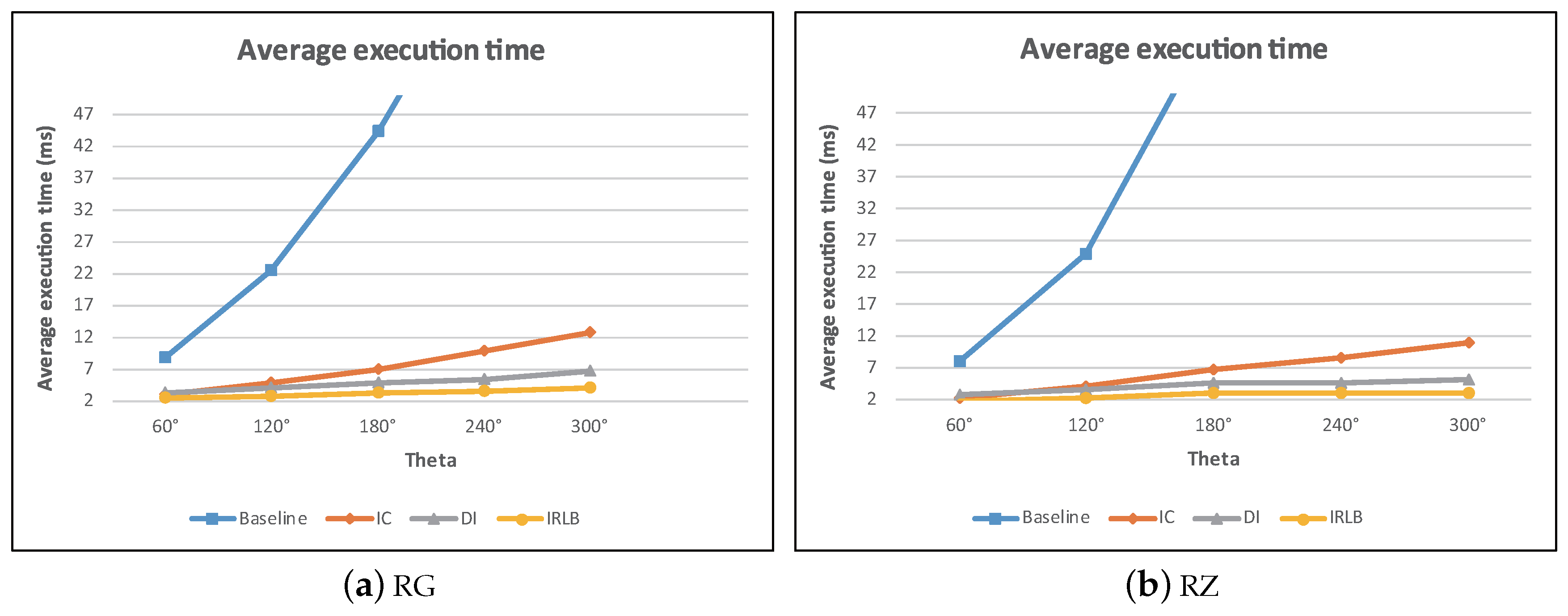
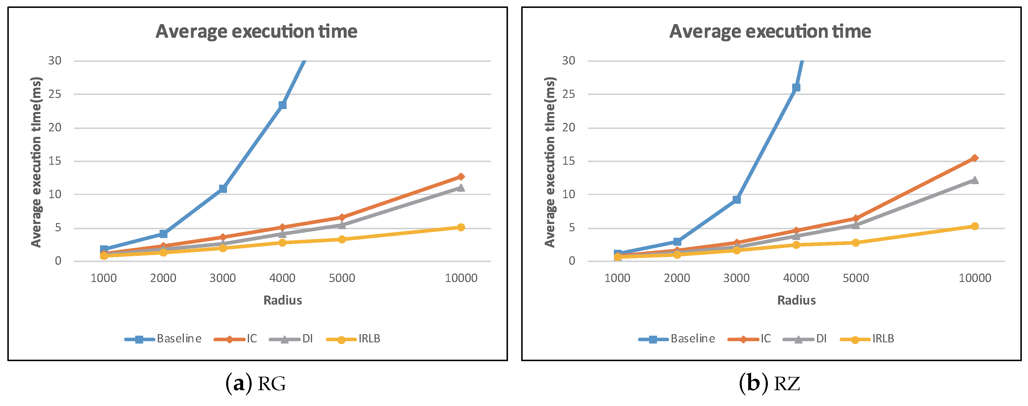
5.6. The Effect of r and $\theta$

In the experiments, we analyzed how the performance was impacted by two parameters: r and $\theta$. The two parameters control the covering area of a view field. The larger the value of r and $\theta$, the more data objects and obstacles are covered by a view field. The results are reported in Figure 27 and Figure 28. The two figures show a very similar trend, that is the larger the size of a view field, the longer the query execution time. Once again, the results show that our pruning techniques can discard many unqualified obstacles so that IC, DI, and IRLB provide acceptable performance even when the view field is large.

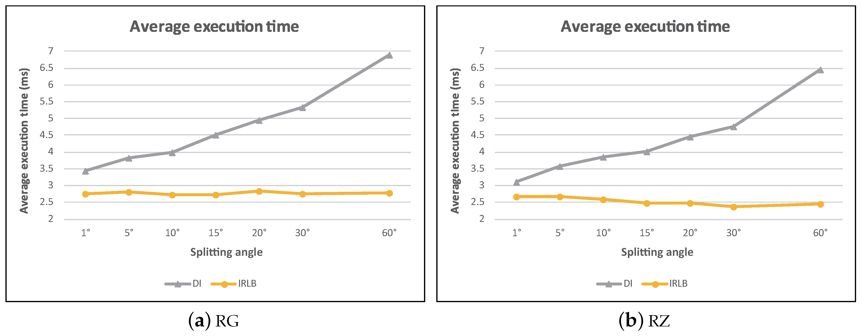
5.7. The Effect of the Splitting Angle $({\theta }_{\mathcal{S}})$

In this experiment, we investigated the effect of ${\theta }_{\mathcal{S}}$, which determines the direction index’s angle range of each section. Since parameter ${\theta }_{\mathcal{S}}$ only affected the performance of DI and IRLB, we omit the simulation results of baseline and IC. By observing Figure 29, we find that the average execution time of DI increased rapidly when ${\theta }_{\mathcal{S}}$ increased. This is because the larger value of ${\theta }_{\mathcal{S}}$ means that a section would cover a wider spatial region, and more obstacles would be contained in a section. Thus, DI had to spend more time to check the visibility of data objects, incurring excessive computational cost.

Although IRLB is based on DI, it uses invisible regions lookup table to perform a two-phase search scheme (see Section 4.4.3). Since the visibility of a large number of data objects is determined by the lookup table (i.e., in phase one), only a few data objects are passed to DI for further processing. This makes IRLB much less sensitive to the increases of ${\theta }_{\mathcal{S}}$.

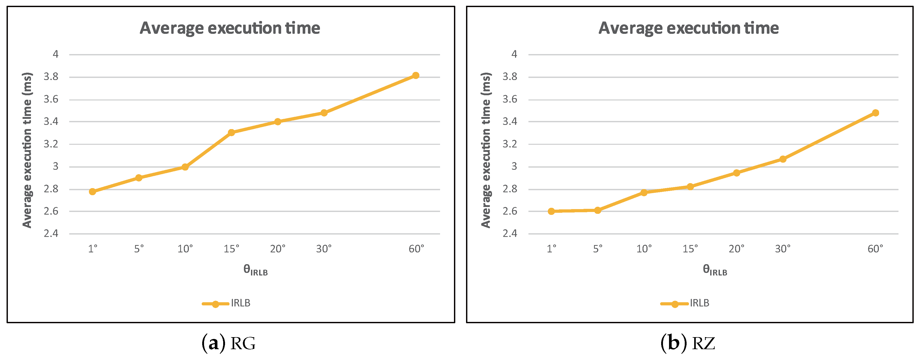
5.8. The Effect of the Slitting Angle $({\theta }_{IRLB})$

Continuing with the previous experiment, with a fixed value of ${\theta }_{\mathcal{S}}$ = ${10}^{\circ }$, we keep investigating the effect of ${\theta }_{IRLB}$. Since ${\theta }_{IRLB}$ is only related to IRLB, we only plot the performance of IRLB in Figure 30. We find that the average execution time of IRLB increased as ${\theta }_{IRLB}$ increased. This is mainly because as ${\theta }_{IRLB}$ became larger, the probability that a region was fully blocked by obstacles became lower. This means that less data objects can be pruned in advance and have to be further examined by DI. With the computational cost of visibility checking increasing, the execution efficiency of IRLB became less effective.

6. Conclusions and Future Work

In this paper, we proposed algorithms for processing V2-kNN queries, which retrieve k visible data objects in the presence of obstacles within user’s view field. Two factors affect the visibility of data objects: (1) the view field and (2) physical obstacles (e.g., buildings, or hills). This paper represents a first attempt at considering both factors in finding the solutions. To make V2-kNN more efficient, we utilized a grid index structure to index data objects and obstacles. Based on the index, we designed four algorithms (i.e., baseline, IC, DI, and IRLB) to process V2-kNN queries. Baseline is the basis for the remaining three algorithms. Baseline uses the grid index to access only cells that overlap with the view field. The core idea of the baseline algorithm is to visit cells from near to the distant according to their distance to q. Without having any pruning heuristics, this algorithm resulted in a quite high execution cost. The IC algorithm extends the baseline algorithm by exploiting the fact that obstacles affecting the visibility of p can only exist in the cells intersecting with $\overline{qp}$ (i.e., the line segment connecting q and p). Thus, IC only checks the cells overlapping $\overline{qp}$. This strategy greatly reduced the number of accessed obstacles, leading to a much more acceptable performance. In the DI algorithm, we devised the “direction index” to index the obstacles within a view field. Based on the direction index, we proved that for p, only obstacles falling within a certain angle may affect the visibility of p (this angle is relative to q). In IRLB, we designed a light-weight data structure to index the invisible areas in the view field. Data objects that fall in the invisible areas cannot be the answer. We used the index structure to discard those invisible data objects quickly when processing a V2-kNN query. Consequently, only a small number of data objects required further processing. Our experiments have demonstrated that all proposed algorithms can achieve our goal, that is finding visible kNN objects in the presence of obstacles within a user’s view field. The results also showed that IC, DI, and IRLB were better than baseline. This proves that the pruning strategies indeed significantly reduced the number of accessed obstacles and data objects. In addition, IRLB performed the best among all the algorithms, manifesting that the angle-based pruning strategy and the two-phase searching scheme were effective, as expected, in cutting down the size of the search space.

This work opens several promising directions. First, the Euclidean distance can be extended to the road network distance, which will require our algorithm to be redesigned to meet the need of road-network applications. Second, it would be interesting to take the dynamic environment into consideration, meaning that data objects and the query point may move and change their direction of movement. Third, as the obstacles are irregular in shape in the real world, we will investigate an efficient approach to check the visibility of objects under such conditions to make the solutions better meet the needs of real life.