Abstract
Uncontrolled and continuous urbanization is an important problem in the metropolitan cities of developing countries. Urbanization progress that occurs due to population expansion and migration results in important changes in the land cover characteristics of a city. These changes mostly affect natural habitats and the ecosystem in a negative manner. Hence, urbanization-related changes should be monitored regularly, and land cover maps should be updated to reflect the current situation. This research presents a comparative evaluation of two classification algorithms, pixel-based support vector machine (SVM) classification and decision-tree-oriented geographic object-based image analysis (GEOBIA) classification, in producing a dynamic land cover map of the Istanbul metropolitan city in Turkey between 2013 and 2017 using Landsat 8 Operational Land Imager (OLI) multi-temporal satellite images. Additionally, the efficiencies of the two data dimension reduction methods are evaluated as part of this research. For dimension reduction, built-up index (BUI) and principal component analysis (PCA) data were calculated for five images during the mentioned period, and the classification algorithms were applied on data stacks for each dimension reduction method. The classification results indicate that the GEOBIA classification of the BUI data set provided the highest accuracy, with a 91.60% overall accuracy and 0.91 kappa value. This combination was followed by the GEOBIA classification of the PCA data set, which highlights the overall efficiency of the GEOBIA over the SVM method. On the other hand, the BUI data set provided more reliable and consistent results for urban expansion classes due to representing physical responses of the surface when compared to the data set of the PCA, which is a spectral transformation method.
1. Introduction
The increase in urbanization and residential areas has been an inevitable process due to economic development and rapid population growth throughout human history [1]. Extreme urbanization, especially in metropolitan cities, causes significant changes in land cover (LC) characteristics [2]. The increase in urbanization also leads to negative consequences, such as ecological deterioration and global warming due to the rapid consumption of natural resources [3,4]. Therefore, the regular follow-up of the current LC and changes in the LC is important for environmental and urban management and planning processes [5].
With developments in satellite systems and technologies in the last 20 years, satellite image based analysis has become an alternative to the classic terrestrial measurements in determining the LC and changes in LC. Moderate and high-spatial-resolution satellite images, which are available free of charge, have become advantageous for terrestrial measurements considering high labor requirements, costs, and temporal burdens [6,7,8]. Specifically, since the 1990s, there have been significant improvements in accessibility and the spectral and spatial resolutions of remote sensing data. Consistent with these developments, important studies have been carried out to determine the LC status in heterogeneous areas [9,10,11,12]. On the other hand, the proposed methods and analyses vary according to the resolution characteristics of the satellite images and the complexity of the targeted LC classes. For this reason, standardized and simplified methods need to be developed to determine the status and changes in LC using remote sensing data in densely populated areas where complex surfaces are present [13].
Pixel-based classification algorithms are frequently used to determine the status of LC from satellite images. Among these algorithms, there are studies indicating that machine learning-based methods, such as support vector machine (SVM), random forest (RF), k-nearest neighbor (kNN), and decision tree (DT) methods, which have increased in usage rate in recent years, provide higher accuracies than traditional algorithms due to their non-parametric structure [14,15,16,17,18,19,20]. Comparative evaluations of machine learning algorithms in LC mapping report similar accuracies for the SVM and RF methods, which outperform other algorithms [18,19,20]. In addition, according to Tanh Noi and Kappas (2018) and Maulik and Chakraborty (2017), the SVM method converges with acceptable accuracy values much faster and with less memory requirement compared to other machine learning-based classifiers for imbalanced data sets, where the amount of training samples is very limited when compared to the whole dataset, similar to the image classification situation [20,21].
In recent years, geographic object-based image analysis (GEOBIA) has become an extensively used classification algorithm, especially after the widespread use of very high-resolution satellite images. The use of this method in the classification of moderate spatial resolution data, such as Landsat, with high accuracy has also become widespread [22,23,24,25]. The main advantage gained by the object-based classification is the segmentation of pixels to form objects, which reduces the within-object heterogeneity problem faced in pixel-based classification methods due to spectral variations in pixels that constitute a single object [26]. In addition, the GEOBIA method enables the use of the non-metric decision tree approach, which takes into account the statistical, geometric, textural, and spectral properties [27].
When the investigation of LC change is of concern, most studies—even recent ones—mainly focused on separately performing the classification of images with different dates and performing a change detection analysis on the thematic maps produced by the classification [28,29,30]. On the other hand, Wulder et al. (2018) [31] pointed out the expansion on the availability of freely available and spatially and spectrally compatible satellite images with Landsat and Sentinel missions, which triggers high temporal and multi-sensor data analysis. With respect to the abovementioned developments in remotely sensed data availability, they proposed a new concept, called “Land Cover 2.0”, which integrates the land change information into the land cover maps by processing dense time series of multispectral data.
The critical issue that should be taken into account when dealing with high temporal satellite image data is the nonlinear and highly correlated structure of such a dataset. Multispectral satellite sensors record electromagnetic radiation from different portions of the spectrum and thus provide high dimensional data with several image bands [32]. Despite the advantages of high dimensional data, the high correlation of pixel values in nearby bands brings out difficulties in classification due to undesired, highly correlated data; high processing time; and high storage needs. Additionally, high dimensionality of the feature space when compared to the limited training samples results in low classification accuracies, which is known as the Hughes effect in the literature [33]. These drawbacks become more evident, when multi-temporal analysis is of concern, due to the increased number of image bands included in the process [34].
At this point, several dimension reduction methods can be used to reduce the number of inputs while keeping the separation capacity of the data at an acceptable level. Spectral index analysis is one of the basic methods used to simplify the complex spectral characteristics of surface coverage types and emphasize specific features. Spectral indices are designed to be sensitive to a particular type of surface cover, such as the vegetation index, built-up index, and water index. In the literature, successful results were obtained with index-based classification approaches for the determination of settlement areas [35,36]. Another way to reduce the data dimension is to apply spectral transformation methods, such as the principal components analysis (PCA) and independent component analysis (ICA), to remove the correlations and higher order dependencies in the image bands and use the produced components as input data for classification [37,38].
The main objective of this research is to produce a land cover map of the Istanbul metropolitan city in Turkey, which shows heterogeneous surface characteristics and faces extensive LC changes due to urbanization and industrial development. This research specifically focusses on introducing a method for the determination of dynamic change classes in addition to static LC classes in a single classification process with the use of multi-temporal satellite images. The critical advantage gained by multi-temporal data is the inclusion of temporal responses of the surface in addition to spectral, textural, and contextual information. Within this context, the performances of two classification algorithms, pixel-based SVM classification and non-parametric decision tree GEOBIA classification, were evaluated. Additionally, this research evaluates the effect of spectral index-based and spectral transformation-based dimension reduction methods, namely, the built-up index and PCA transformation, on the classification process.
2. Study Area and Data
Istanbul is a metropolitan city that has been exposed to continuous urbanization, with a prominent position that connects the European and Asian continents economically and culturally. It is the most crowded city in Turkey and one of the largest metropolitan areas in Europe. The city covers an area of 5500 square kilometers, and according to the national population statistics released in 2017, it hosts 15 million residents, which corresponds to 18% of the country [39].
Specifically, in the second half of the 20th century, industrial development and uncontrolled urbanization due to migration resulted in extensive changes in the land cover structure and morphology of the city [40]. Increasing urbanization in Istanbul and the related changes in LC since the beginning of the 2000s attracted the attention of many researchers.
Many studies have been carried out to determine the current LC situation and changes in LC using satellite images. These studies, which were performed with use of pixel-based classification algorithms, indicate that there has been a significant decrease in natural surface cover types due to the intense increase in residential areas [8,41,42,43].
Within the last decade, three important infrastructures have been constructed, which are the Yavuz Sultan Selim Bridge, the Black Sea Highway, and the Istanbul International Airport, to strengthen the transportation network. These constructions have direct and indirect impacts on the ecosystem by increasing the number of impervious surfaces and making their surroundings a center of attraction for new settlements, respectively. Specifically, the northern part of the city is affected negatively by this phenomenon due to decrease in forest and natural lands (Figure 1).
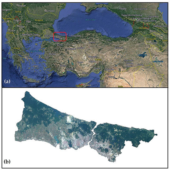
Figure 1.
Study sites and overview of the images used in this research: (a) Geographic location of Turkey (Google Earth©). (b) Overview of Istanbul city from 2017-dated Landsat 8 data.
The Landsat 8 satellite images that cover the administrative borders of the city, which were acquired between 2013 and 2017, were used in this research. The selected images were acquired in the summer and early fall seasons to minimize seasonal effects and ensure the regularity of the temporal interval. The OLI sensor onboard the Landsat 8 satellite provides eight spectral channels with a 30 m spatial resolution and a single panchromatic channel with a 15 m spatial resolution. Additionally, two thermal channels are provided from the TIRS sensor, which are acquired with a 100 m native resolution and resampled to 30 m. The spatial coverage of the images acquired by the satellite is 170 × 183 km [44]. The images are distributed by USGS at the L1TP processing level, which includes basic radiometric calibration and orthorectification steps. In the orthorectification step, ground control points and the Global Land Survey (GLS) 2000 digital elevation model are used to ensure high positional accuracy and accurate terrain correction. The properties of the satellite images used in this research are presented in Table 1.

Table 1.
Specifications of the Landsat 8 OLI satellite images used in this study.
Google Earth was used for reference data in the training data selection and accuracy assessment steps, as it provides very high-resolution imagery of a region at the required time interval.
3. Methodology
3.1. Preprocessing of the Satellite Images
The Landsat 8 image pixels are delivered as quantized digital numbers (DNs), which represent the brightness values. Within the context of multi-temporal satellite image analysis, it is necessary to convert the values from brightness values to top of atmosphere (ToA) values to minimize the differences in the illumination and reflectance properties that occur due to the image detection date and to perform analyses at the equivalent radiometric scale [45]. This conversion was performed using parameters provided with the metadata file of the Landsat 8 satellite images and the following formula set [46]:
where
ρλ′ = MρQcal + Aρ
- ρλ′ = ToA planetary spectral reflectance without correction for the solar angle (unitless)
- Mρ = Reflectance multiplicative scaling factor for the band
- Aρ = Reflectance additive scaling factor for the band
- Qcal = L1 pixel value in the DN
This process does not include correction for the solar elevation angle. The following additional formula is used to obtain the true ToA reflectance:
where
ρλ = ρλ′/sin(ƟSE)
- ρλ = ToA Planetary Reflectance (unitless)
- ƟSE = Solar Elevation Angle
After the radiometric calibration process, the ToA images are recorded as float data.
The second step of pre-processing is pan-sharpening of the Landsat 8 images. For this purpose, the Gram–Schmidt spectral pan-sharpening algorithm was used. In this algorithm, an artificial panchromatic channel is derived from the low-spatial-resolution multispectral channels in the first stage. In the second stage, the Gram–Schmidt transformation is applied to the artificial panchromatic channel and multispectral channels. In the third stage, the first Gram–Schmidt channel is displaced with high-spatial-resolution panchromatic data. In the last stage, the inverted Gram–Schmidt transform is applied to the data set to obtain pan-sharpened spectral channels [47]. The main advantage of the algorithm lies behind the procedure, which performs orthogonalization after weighting each multispectral image channel based on its spectral formation with panchromatic data, thus allowing all of the low-resolution multispectral image channels, including the shortwave infrared (SWIR) channel, to be included in the process. In the last step, pan-sharpened images were clipped with administrative boundary vector data of the Istanbul metropolitan city.
3.2. Dimension Reduction
The first approach that was evaluated in this research is the spectral index-based method. As this research mainly concentrated on evaluating the LC changes due to urbanization, the built-up index-based approach was adopted. The normalized difference built-up index (NDBI) is one of the first introduced indexes [48]. The NDBI was modified by integration of the normalized difference vegetation index (NDVI), which is referred to as the built-up index (BUI). Previous studies with BUI data reported that this index improves the separation between urban areas and bare lands [49]. Equation (3) provides the calculation of the BUI.
where SWIR corresponds to the shortwave infrared band, NIR corresponds to the near infrared band and RED corresponds to the red image band.
BUI = ((SWIR − NIR)/(SWIR + NIR) − ((NIR − RED)/(NIR + RED))
BUI data were calculated from the satellite images and stored as a single band.
The second approach evaluated in this research is the principal component analysis (PCA)-based spectral transformation method. This method performs a rotation of the axes of the original feature space coordinate system to new orthogonal axes called principle axes, which maximizes the data variance [50]. In general, 90% of the variance is stored in the first three axes, and variance reduces with increasing axis number [51]. In this research, the first component is calculated for each satellite image and stored as a single data layer.
After dimension reduction, the BUI and PCA data were layer-stacked according to the date order and recorded as unsigned 8-bit data (Figure 2).

Figure 2.
Red/Green/Blue (RGB) view of the dimension reduction results: (a) built-up index (BUI) layer stack and (b) principal component analysis (PCA) layer stack (R: 2013/G: 2015/B: 2017).
3.3. Land Cover Classes
The LC classes used in this research were defined by taking the Anderson (1976) LC legend as the basis and by taking into account the resolving capacity of the Landsat 8 OLI images with a 15 m resolution [52]. Additionally, two change classes were included to define classes, with inspiration from the “Land Cover 2.0” concept introduced by Wulder et al. (2018), in which dynamic change classes are evaluated together with the main LC classes in a single classification [31]. In this context, the classes and their definitions are given in Table 2.
Table 2.
Definitions of the land cover classes mapped in this research.
3.4. Classification
This research evaluated two state of the art classification methods for mapping the current LC and its changes during a 5-year period. The first method used in this study was based on pixel-based supervised implementation of the SVM algorithm. The SVM uses an iterative learning process to define linear hyperplanes for separation between classes [53]. The initial implementation of the SVM was working as a binary classifier, and a pairwise classification approach was developed to cope with multiclass processing requirements, such as satellite image classification [54]. Additionally, the SVM algorithm provides better results than the traditional classifiers, such as the maximum likelihood classifier, when the input data are non-Gaussian, such as in satellite images, due to its non-parametric structure [55]. Moreover, the SVM algorithm requires less training data than other machine learning classifiers, which require intensive training samples for high-dimensional input data [56]. The learning of hyperplanes in a higher dimensional space is achieved by kernel-based transformation. This research uses the radial basis function (RBF) kernel due to its reported higher performance with non-linear datasets and lower computational complexity [57,58].
The training samples were selected manually within the stacked images, with a simultaneous check from Google Earth. The number of training samples was decided simply according to the areal coverage and fuzziness of the LC class. The distribution of the training samples is summarized as follows: Built-up Lands (657 polygons—95,705 pixels), Agricultural Lands (105 polygons—131,192 pixels), Forests (298 polygons—90,131 pixels), Bare and Semi-Natural Lands (51 polygons—12,964 pixels), Water Bodies (68 polygons—42,000 pixels), Urban Expansion 1 (314 polygons—21,755 pixels), and Urban Expansion 2 (210 polygons—17,143 pixels). The spectral separability of the training samples across different classes is an important metric that represents how well the selected samples pair statistically. The tool included in the ENVI@ software calculates the pairwise separation metric based on both the Jeffries–Matusita and transformed divergence separability measures [51,59]. This metric can take values between 0 and 2, where values greater than 1.5 indicate good separation. Table A1 provides the pairwise separation values calculated for the BUI and PCA data sets for all possible class combinations. Additionally, Table 3 provides detailed parameter values for the SVM classification applied to the stacked datasets. The first two parameters given in the Table 3 are generic parameters of the SVM algorithm, while the remaining ones belong to software specific parameters of the classification process. The Gamma parameter is calculated as the inverse of the number of image bands. The penalty parameter is set to 100 to avoid misclassification at the training step. The classification probability threshold ensures that all of the pixels are assigned to a class when set to a value of 0. A pyramid level value greater than 0 allows for classification to be performed on a low-resolution pyramid image, and if the class probability of a pixel is lower than the pyramid reclassification threshold, the pixel will be reclassified at a finer resolution [60].
Table 3.
Definition of the parameters used for SVM classification in ENVI@ software.
The second classification method evaluated in this research is the threshold-based decision tree GEOBIA approach. The adaptation of the non-parametric statistical decision tree technique to object-based classification has been performed successfully to determine LC mapping in past decades [20,61,62,63].
The GEOBIA classification consists of two steps. In the first step, segmentation of the multi-layered data set produces segments that represent a meaningful Earth object either alone or in groups. In the segmentation process, scale, color, shape, and texture parameters are considered [64,65,66]. In the second step, hierarchical or relational class definitions are structured according to the reflectance, shape and texture characteristics of the segments [67,68].
The multiresolution segmentation algorithm implemented via eCognitionTM software was used in this research. The algorithm aims to determine the most appropriate scale parameter for the whole area based on the necessity of expressing different objects at different scales in line with the size and texture characteristics. The scale parameter controls the amount of spectral variation in the pixel group to create the object and resulting segment size. The first of the two complementary parameter sets in the segmentation process is the Shape—Color component. Shape and color are defined to complement each other at a value of 1, and the importance of these parameters in determining the object boundaries is determined by this weighting. The shape features are determined by the sub-complementary parameters, which are compactness and smoothness [69]. Different parameter combinations were experimented on the BUI and PCA datasets, and the parameters producing the objects, in which the surface cover types were significantly represented, were determined. In this context, the most appropriate segmentation is provided by the following parameter set: scale factor: 20; shape: 0.2; and compactness: 0.5.
The second step of the process is to determine the thresholds for class definitions based on the spectral, textural and temporal characteristics of the segments and to build hierarchical relationships of the classes. The thresholds were defined using the mean values for each data layer, the maximum difference, grey level co-occurrence (GLCM) homogeneity and GLCM dissimilarity parameters, which were obtained from image segments and variations in these parameters through the temporal domain. The detailed calculation steps of the GLCM texture parameters can be found in the work performed by Haralick et al. in 1973 [70].
The thresholds were defined by examining the abovementioned segment parameters at approximate locations of the training dataset used in the SVM approach with a simultaneous check from Google Earth. Then, iterative fine-tuning was performed on the thresholds by visual inspection of class coverage across the whole dataset. The final class definitions and decision tree structures for the BUI and PCA datasets are presented in Figure A1 and Figure A2, respectively.
3.5. Accuracy Assessment
An accuracy assessment of the classification results was performed with two different assessment approaches. In the first approach, a point-based traditional accuracy assessment procedure was performed by use of 250 stratified random points. The distribution of points was determined by taking into account class coverage and class heterogeneity [71]. The error matrix was created by means of class labels and corresponding reference labels [72]. User and producer accuracy measures and kappa statistics are derived from these matrices [73,74].
As a second assessment method, the intersection of the area relative to the reference polygon was used. This method performs an area-based ratio calculation between the intersected area from the results to the reference polygon area (Aint/Aref) [75,76]. This method is used for evaluating the segmentation accuracy and can be implemented on the classification accuracy simply by converting the classification results into vector data and extracting the intersection with reference polygons. For this purpose, 25 reference polygons were extracted for each class from Google Earth, and these polygons were intersected with the classification vector. The ratio can take values from 0 (where the pixels or segment under the reference polygon is completely misclassified) to 1 (where the pixels or segment under the reference is completely true). After the ratio calculation, the mean and standard deviation metrics were provided for each class and for all classification method—dimension reduction method combinations.
4. Results and Discussion
4.1. Experimental Results
The LC maps produced by GEOBIA and SVM classification of the BUI and PCA datasets are presented in Figure A3, Figure A4, Figure A5 and Figure A6. Moreover, the point-based accuracy assessment results are presented in Table 4. When these results are evaluated, it can be seen that the GEOBIA method produced thematically homogenous maps when compared to the SVM method for both datasets. The SVM method especially suffered from the misclassification of uncultivated agricultural lands as built-up areas, which is observable in the western part of the province. Nevertheless, the overall accuracies achieved with the SVM classification results are within the same ranges as those in previous studies, such as Tanh Noi and Kappas [20]. The GEOBIA method takes advantage of including textural information from these regions (homogeneity for BUI—homogeneity, dissimilarity and homogeneity for PCA), where reduced spectral information was similar. Moreover, the segmentation process in the GEOBIA enables higher quality object boundary definition that reduces within object heterogeneity, thus provides better thematic object representation.
Table 4.
Point-based accuracy results (PA: Producer Accuracy; UA: User Accuracy; K: Kappa).
When the dimension reduction methods were evaluated, the classification results from the BUI dataset provided higher accuracies when compared to the PCA dataset, except for the water body class. The lower accuracy of the water body class occurred due to similar multi-temporal responses of shallow water areas and urban areas, which could be partially solved in the GEOBIA method by adding the homogeneity parameter to the class definition but remained a problem in the SVM classification. In addition, the higher accuracies obtained for urban expansion classes with the BUI dataset indicate superiority of the BUI dimension reduction method over the PCA method, especially when change detection is the main concern. The main concern with the BUI-based method was its efficiency to differentiate different land cover classes, as it was initially designed to determine built-up areas. However, its stable and meaningful responses to different land cover types through the time domain pointed out the effective usage in land cover mapping when multi-temporal satellite images are available.
Although point-based accuracy metrics are well-known and intensely used parameters for evaluating the accuracy of image classifications, information about the thematic representation quality of land objects cannot be retrieved with these metrics. Thus, a polygon-based evaluation can be more useful to derive the thematic accuracy of object representation. According to the polygon-based accuracy analysis presented in Table 5, it can be seen that the GEOBIA-based classification results provided higher accuracies in object representation, with higher mean values and comparatively lower standard deviations. Additionally, the number of polygons with representation ratios below 50% was smaller for the GEOBIA results when compared to the SVM results. The GEOBIA classification of the BUI dataset provided the highest ratios for all classes, and the ratio ranges across classes were mostly stable. The PCA-GEOBIA combination was ranked second, which was followed by the BUI-SVM and PCA-SVM combinations. These results are consistent with the point-based accuracy analysis.
Table 5.
Polygon-based accuracy results (Mean: Mean value of Aint/Aref; Std: Standard deviation of Aint/Aref; C: Count for Aint/Aref ≤ 0.50).
The areal statistics were extracted from the classification results, and relative differences were calculated by taking the BUI-GEOBIA classification as the reference, due to its highest point-based and polygon-based accuracy metrics (Table 4 and Table 5). According to this comparison, GEOBIA classification of the PCA dataset provided similar areal information, with relative differences below 10%; however, the SVM classification of both datasets provided over 10% differences specific to agricultural land, water body and urban expansion classes (Table 6).
Table 6.
Areal statistics and relative differences calculated from the classification results.
Evaluations on the current areal status of LC and urban expansion classes from the BUI-GEOBIA classification results (Table 6), inform that a total urban expansion of 14,427.97 ha that occurred during a five-year period corresponded to a 14.43% increase in urban areas when the built-up lands class is taken as the reference. In addition, this expansion amount corresponds to 2.7% of the total province area, which can be considered as an important urbanization process for a short time period. The forests cover 41.5% of the province area and are located in the northern part of the province, while extensive built-up lands and agricultural lands mostly cover the southern part of the province.
Urban expansion that occurred during the analysis period mainly originated from the construction of the Istanbul International Airport, Yavuz Sultan Selim Bridge, Black Sea Transit Highway and connection roads to these transportation facilities. It is crucial that all of these constructions are located along the northern axis of the province, where forests and natural lands exist. There is a need for the continuous monitoring and management of lands near these facilities, as these regions are candidates for uncontrolled urbanization.
4.2. Discussion on Possible Limitations and Error Sources
When the results are evaluated, it can be strongly suggested that GEOBIA-based non-parametric classification method provided higher accuracies in both BUI and PCA datasets, due to the capability of including textural parameters in addition to spectral information. On the other hand, it should be noted that the segmentation process directly affects the thematic accuracy of the GEOBIA-based classification. The segmentation accuracy was not evaluated directly on this research; however, the polygon-based accuracy assessment results demonstrated higher accuracies for the GEOBIA classification results, which may indicate acceptable performance of segmentation in object representation.
Another challenging step in the non-metric GEOBIA-based classification approach was determining the parameter thresholds for class definitions. During this process, several segments belonging to specific classes were determined with validation from Google Earth reference data, and parameter thresholds were examined through these sample segments. At this point, the threshold definition from the BUI dataset was less complicated, as the BUI represents normalized physical responses of the surface reflectance characteristics, while the PCA provides a statistical dissimilarity measure of the pixels throughout the image domain. In addition, although the BUI is mainly focused on highlighting urban areas, the responses of the BUI dataset for other classes in the time domain also provided more understandable and robust characteristics than the PCA dataset. The only drawback of the BUI dataset was similar spectral responses of shallow water bodies and urban areas, which was overcome by the use of the homogeneity parameter in the GEOBIA classification. Additionally, the PCA dataset generally required more complex class definitions with the implementation of more GLCM textural parameters.
The main constraint observed in the pixel-based SVM classification process is that only the spectral features derived from the dimension reduction process can be included in the process. The similarity of the responses from different LC surfaces, both in the scene and time domains, had a direct effect on the classification accuracy. The separation metrics calculated from the training samples (Table A1) provided a positive correlation with the accuracy assessment results, which indicated that they can be used as pre-estimators of the classification efficiency before performing the whole process.
Specifically, the mixed responses of shallow water and urban areas in the BUI dataset were evident in the SVM classification and resulted with the false classification of shallow water areas as urban class areas, especially over the coasts of lakes. Second, the mixed response of built-up areas and agricultural lands resulted with the misclassification of some agricultural lands as built-up areas in the midwest part of the study area.
5. Conclusions
The results of the study show that the Istanbul province has been exposed to LC changes in the form of urban expansion during the last five years. The main source of urban expansion is the constructions of the new airport, new bridge and new connection highways to these transportation facilities. In addition, the construction of new settlements also contributes to the expansion of urban areas. This change causes the destruction of forest areas and natural areas, especially in the northern half of Istanbul. This amount of change has a high potential for generating negative impacts on the natural environment and ecosystem. The findings of this research and the proposed non-parametric decision-tree-based GEOBIA classification approach can be useful in providing a periodically updated geospatial LC database, which can be used in the management activities of decision makers, thanks to its capacity to detect time-dependent changes in a fast and reliable manner. Additional studies plan to enhance this research by the use of images from different satellites, such as Sentinel 2, which provide higher spatial, spectral and temporal resolutions and the evaluation of different dimension reduction techniques to improve the accuracy and reliability of dynamic LC maps produced from satellite images.
Author Contributions
Formal analysis, Ugur Alganci; Methodology, Ugur Alganci; Validation, Ugur Alganci; Visualization, Ugur Alganci; Writing—original draft, Ugur Alganci.
Funding
This research received no external funding.
Acknowledgments
The author acknowledges the support of the Istanbul Technical University—Center for Satellite Communications and Remote Sensing (ITU-CSCRS) for providing the licensed software and computing environment and the United States Geological Survey (USGS) for providing the Landsat 8 satellite images free of charge. The author thanks the anonymous reviewers, who helped improve the quality of this research with their valuable comments.
Conflicts of Interest
The authors declare no conflict of interest.
Appendix A

Figure A1.
Threshold-based decision tree structure for the BUI dataset.

Figure A2.
Threshold-based decision tree structure for the PCA dataset.

Figure A3.
GEOBIA classification results of the BUI dataset.

Figure A4.
GEOBIA classification results of the PCA dataset.

Figure A5.
SVM classification results of the BUI dataset.

Figure A6.
SVM classification results of the PCA dataset.
Table A1.
Separation metrics derived from training samples for the BUI and PCA datasets.
Table A1.
Separation metrics derived from training samples for the BUI and PCA datasets.
| BUI | PCA | ||
|---|---|---|---|
| Pair Separation (Least to Most) | Value | Pair Separation (Least to Most) | Value |
| Built-up Lands and Water Bodies | 1.15 | Built-up Lands and Agricultural Lands | 1.31 |
| Agricultural Lands and Urban Expansion 1 | 1.70 | Agricultural Lands and Bare and Semi-Natural Lands | 1.51 |
| Built-up Lands and Agricultural Lands | 1.72 | Built-up Lands and Bare and Semi-Natural Lands | 1.55 |
| Water Bodies and Agricultural Lands | 1.75 | Agricultural Lands and Urban Expansion 1 | 1.65 |
| Agricultural Lands and Bare and Semi-Natural Lands | 1.85 | Built-up Lands and Urban Expansion 2 | 1.66 |
| Water Bodies and Urban Expansion 1 | 1.85 | Agricultural Lands and Urban Expansion 2 | 1.66 |
| Built-up Lands and Urban Expansion 1 | 1.88 | Forests and Urban Expansion 2 | 1.67 |
| Urban Expansion 2 and Bare and Semi-Natural Lands | 1.89 | Urban Expansion 2 and Bare and Semi-Natural Lands | 1.72 |
| Built-up Lands and Bare and Semi-Natural Lands | 1.93 | Built-up Lands and Urban Expansion 1 | 1.82 |
| Urban Expansion 1 and Urban Expansion 2 | 1.94 | Urban Expansion 1 and Urban Expansion 2 | 1.82 |
| Agricultural Lands and Urban Expansion 2 | 1.95 | Forests and Agricultural Lands | 1.94 |
| Forests and Urban Expansion 2 | 1.95 | Forests and Built-up Lands | 1.95 |
| Built-up Lands and Urban Expansion 2 | 1.96 | Urban Expansion 1 and Bare and Semi-Natural Lands | 1.96 |
| Urban Expansion 1 and Bare and Semi-Natural Lands | 1.98 | Forests and Urban Expansion 1 | 1.98 |
| Water Bodies and Bare and Semi-Natural Lands | 1.99 | Built-up Lands and Water Bodies | 1.98 |
| Forests and Built-up Lands | 2.00 | Water Bodies and Urban Expansion 2 | 2.00 |
| Water Bodies and Urban Expansion 2 | 2.00 | Forests and Bare and Semi-Natural Lands | 2.00 |
| Forests and Agricultural Lands | 2.00 | Water Bodies and Urban Expansion 1 | 2.00 |
| Forests and Urban Expansion 1 | 2.00 | Forests and Water Bodies | 2.00 |
| Forests and Bare and Semi-Natural Lands | 2.00 | Water Bodies and Agricultural Lands | 2.00 |
| Forests and Water Bodies | 2.00 | Water Bodies and Bare and Semi-Natural Lands | 2.00 |
References
- Shalaby, A.; Aboel Ghar, M.; Tateishi, R. Desertification impact assessment in Egypt using low resolution satellite data and GIS. Int. J. Environ. Stud. 2004, 61, 375–384. [Google Scholar] [CrossRef]
- Yuan, F.; Sawaya, K.E.; Loeffelholz, B.C.; Bauer, M.E. Land cover classification and change analysis of the Twin Cities (Minnesota) Metropolitan Area by multi-temporal Landsat remote sensing. Remote Sens. Environ. 2005, 98, 317–328. [Google Scholar] [CrossRef]
- Finkl, C.W.; Charlier, R.H. Sustainability of subtropical coastal zones in southeastern Florida: Challenges for urbanized coastal environments threatened by development, pollution, water supply, and storm hazards. J. Coast. Res. 2003, 19, 934–943. [Google Scholar]
- Shi, H.; Singh, A. Status and interconnections of selected environmental issues in the global coastal zones. AMBIO 2003, 32, 145–152. [Google Scholar] [CrossRef] [PubMed]
- Niemi, G.; Wardrop, D.; Brooks, R.; Anderson, S.; Brady, V.; Paerl, H.; Rakocinski, C.; Brouwer, M.; Levinson, B.; McDonald, M. Rationale for a new generation of ecological indicators for coastal waters. Environ. Health Perspect. 2004, 112, 979–986. [Google Scholar] [CrossRef] [PubMed]
- Wardell, D.A.; Reenberg, A.; Tøttrup, C. Historical footprints in contemporary land use systems: Forest cover changes in savannah woodlands in the Sudano-Sahelian zone. Glob. Environ. Chang.-Hum. Policy Dimens. 2003, 13, 235–254. [Google Scholar] [CrossRef]
- Ruiz-Luna, A.; Berlanga-Robles, C.A. Land use, land cover changes and coastal lagoon surface reduction associated with urban growth in northwest Mexico. Landsc. Ecol. 2003, 18, 159–171. [Google Scholar] [CrossRef]
- Kaya, S.; Curran, P. Monitoring urban growth on the European side of the Istanbul metropolitan area: A case study. Int. J. Appl. Earth Obs. 2006, 8, 18–25. [Google Scholar] [CrossRef]
- Barnsley, M.J.; Barr, S.L. Inferring urban land use from satellite sensor images using kernel based spatial reclassification. Photogramm. Eng. Remote Sens. 1996, 62, 949–958. [Google Scholar]
- Herold, M.; Liu, X.; Clarke, K.C. Spatial metrics and image texture for mapping urban land use. Photogramm. Eng. Remote Sens. 2003, 69, 991–1002. [Google Scholar] [CrossRef]
- O’Hara, C.G.; King, J.S.; Cartwright, J.H.; King, R.L. Multitemporal land use and land cover classification of urbanized areas within sensitive coastal environments. IEEE Trans. Geosci. Remote Sens. 2003, 41, 2005–2014. [Google Scholar] [CrossRef]
- Schmidt, K.S.; Skidmore, A.K.; Kloosterman, E.H.; Van Oosten, H.; Kumar, L.; Jannsen, J.A.M. Mapping coastal vegetation using an expert system and hyperspectral imagery. Photogramm. Eng. Remote Sens. 2004, 70, 703–715. [Google Scholar] [CrossRef]
- Campbell, J.B. Introduction to Remote Sensing, 3rd ed.; Guiford Press: New York, NY, USA, 2002. [Google Scholar]
- Bruzzone, L.; Persello, C. A novel context-sensitive semisupervised SVM classifier robust to mislabeled training samples. IEEE Trans. Geosci. Remote Sens. 2009, 47, 2142–2154. [Google Scholar] [CrossRef]
- Mountrakis, G.; Im, J.; Ogole, C. Support vector machines in remote sensing: A review. ISPRS J. Photogramm. Remote Sens. 2011, 66, 247–259. [Google Scholar] [CrossRef]
- Shao, Y.; Lunetta, R.S. Comparison of support vector machine, neural network, and CART algorithms for the land-cover classification using limited training data points. ISPRS J. Photogramm. Remote Sens. 2012, 70, 78–87. [Google Scholar] [CrossRef]
- Khatami, R.; Mountrakis, G.; Stehman, S.V. A meta-analysis of remote sensing research on supervised pixel-based land cover image classification processes: General guidelines for practitioners and future research. Remote Sens. Environ. 2016, 177, 89–100. [Google Scholar] [CrossRef]
- Adam, E.; Mutanga, O.; Odindi, J.; Abdel-Rahman, E.M. Land-use/cover classification in a heterogeneous coastal landscape using RapidEye imagery: Evaluating the performance of random forest and support vector machines classifiers. Int. J. Remote Sens. 2014, 35, 3440–3458. [Google Scholar] [CrossRef]
- Ghosh, A.; Joshi, P.K. A comparison of selected classification algorithms for mapping bamboo patches in lower Gangetic plains using very high resolution WorldView 2 imagery. Int. J. Appl. Earth Obs. Geoinf. 2014, 26, 298–311. [Google Scholar] [CrossRef]
- Thanh Noi, P.; Kappas, M. Comparison of Random Forest, k-Nearest Neighbor, and Support Vector Machine Classifiers for Land Cover Classification Using Sentinel-2 Imagery. Sensors 2018, 18, 18. [Google Scholar] [CrossRef]
- Maulik, U.; Chakraborty, D. Remote Sensing Image Classification: A survey of support-vector-machine-based advanced techniques. IEEE Geosci. Remote Sens. Mag. 2017, 5, 33–52. [Google Scholar] [CrossRef]
- Kim, M.; Madden, M.; Warner, T.A. Forest type mapping using object-specific texture measures from multispectral Ikonos Imagery: Segmentation quality and image classification issues. Photogramm. Eng. Remote Sens. 2009, 75, 819–829. [Google Scholar] [CrossRef]
- Tansey, K.; Chambers, I.; Anstee, A.; Denniss, A.; Lamb, A. Object-oriented classification of very high resolution airborne imagery for the extraction of hedgerows and field margin cover in agricultural areas. Appl. Geogr. 2009, 29, 145–157. [Google Scholar] [CrossRef]
- Chaofan, W.; Jinsong, D.; Ke, W.; Ligang, M.; Tahmassebi, A.R.S. Object-based classification approach for greenhouse mapping using Landsat-8 imagery. Int. J. Agric. Biol. Eng. 2016, 9, 79–88. [Google Scholar]
- Minaei, M.; Kainz, W. Watershed Land Cover/Land Use Mapping Using Remote Sensing and Data Mining in Gorganrood, Iran. ISPRS Int. J. Geo-Inf. 2016, 5, 57. [Google Scholar] [CrossRef]
- Alganci, U.; Sertel, E.; Ozdogan, M.; Ormeci, C. Parcel-Level Identification of Crop Types Using Different Classification Algorithms and Multi-Resolution Imagery in Southeastern Turkey. Photogramm. Eng. Remote Sens. 2013, 79, 1053–1065. [Google Scholar] [CrossRef]
- Duveiller, G.; Defourny, P. A conceptual framework to define the spatial resolution requirements for agricultural monitoring using remote sensing. Remote Sens. Environ. 2010, 114, 2637–2650. [Google Scholar] [CrossRef]
- Subasinghe, S.; Estoque, R.C.; Murayama, Y. Spatiotemporal Analysis of Urban Growth Using GIS and Remote Sensing: A Case Study of the Colombo Metropolitan Area, Sri Lanka. ISPRS Int. J. Geo-Inf. 2016, 5, 197. [Google Scholar] [CrossRef]
- Zhang, J.; Mei, Y. Integrating Logistic Regression and Geostatistics for User-Oriented and Uncertainty-Informed Accuracy Characterization in Remotely-Sensed Land Cover Change Information. ISPRS Int. J. Geo-Inf. 2016, 5, 113. [Google Scholar] [CrossRef]
- Wang, J.; Maduako, I.N. Spatio-temporal urban growth dynamics of Lagos Metropolitan Region of Nigeria based on Hybrid methods for LULC modeling and prediction. Eur. J. Remote Sens. 2018, 51, 251–265. [Google Scholar] [CrossRef]
- Wulder, M.A.; Coops, N.C.; Roy, D.P.; White, J.C.; Hermosilla, T. Land cover 2.0. Int. J. Remote Sens. 2018, 39, 4254–4284. [Google Scholar] [CrossRef]
- Landgrebe, D.A. Signal Theory Methods in Multispectral Remote Sensing; Wiley: Hoboken, NJ, USA, 2003. [Google Scholar]
- Hughes, G. On the mean accuracy of statistical pattern recognizers. IEEE Trans. Inf. Theory 1968, 14, 55–63. [Google Scholar] [CrossRef]
- Abd El-Kawy, O.R.; Rød, J.K.; Ismail, H.A.; Suliman, A.S. Land use and land cover change detection in the western Nile delta of Egypt using remote sensing data. Appl. Geogr. 2011, 31, 483–494. [Google Scholar] [CrossRef]
- Chen, X.-L.; Zhao, H.-M.; Li, P.-X.; Yin, Z.-Y. Remote sensing image-based analysis of the relationship between urban heat island and land use/cover changes. Remote Sens. Environ. 2006, 104, 133–146. [Google Scholar] [CrossRef]
- Zhou, Y.; Yang, G.; Wang, S.; Wang, L.; Wang, F.; Liu, X. A new index for mapping built-up and bare land areas from Landsat-8 OLI data. Remote Sens. Lett. 2014, 5, 862–871. [Google Scholar] [CrossRef]
- Deng, J.S.; Wang, K.; Deng, Y.H.; Qi, G.J. PCA-based land-use change detection and analysis using multitemporal and multisensor satellite data. Int. J. Remote Sens. 2008, 29, 4823–4838. [Google Scholar] [CrossRef]
- Ozdogan, M. The spatial distribution of crop types from MODIS data: Temporal unmixing using Independent Component Analysis. Remote Sens. Environ. 2010, 114, 1190–1204. [Google Scholar] [CrossRef]
- Turkish Statistical Institute (TurkStat). Available online: www.turkstat.gov.tr/ (accessed on 30 June 2018).
- Kaya, S. Multitemporal analysis of rapid urban growth in Istanbul using remotely sensed data. Environ. Eng. Sci. 2007, 24, 228–233. [Google Scholar] [CrossRef]
- Goksel, C.; Kaya, S.; Musaoglu, N. Using satellite data for land use change detection: A case study for Terkos water basin. In Proceedings of the 21st EARSeL Symposium, Paris, France, 14–16 May 2001; Balkema, A.A., Ed.; pp. 299–302. [Google Scholar]
- Coskun, H.G.; Alganci, U.; Usta, G. Analysis of Land Use Change and Urbanization in the Kucukcekmece Water Basin (Istanbul, Turkey) with Temporal Satellite Data using Remote Sensing and GIS. Sensors 2008, 8, 7213–7223. [Google Scholar] [CrossRef] [PubMed]
- Canaz, S.; Aliefendioglu, Y.; Tanrivermis, H. Change detection using Landsat images and an analysis of the linkages between the change and property tax values in the Istanbul Province of Turkey. J. Environ. Manag. 2017, 200, 446–455. [Google Scholar] [CrossRef] [PubMed]
- Barsi, J.A.; Lee, K.; Kvaran, G.; Markham, B.L.; Pedelty, J.A. The spectral response of the Landsat-8 Operational Land Imager. Remote Sens. 2014, 6, 10232–10251. [Google Scholar] [CrossRef]
- Song, C.; Woodcock, C.E.; Seto, K.C.; Lenney, M.P.; Macomber, S.A. Classification and change detection using Landsat TM data: When and how to correct atmospheric effect? Remote Sens. Environ. 2001, 75, 230–244. [Google Scholar] [CrossRef]
- Landsat Handbook. Landsat 8 (L8) Data Users Handbook; LSDS-1574 Version 2.0; USGS-EROS: Sioux Falls, SD, USA, 2016.
- Laben, C.A.; Brower, B.W. Process for Enhancing the Spatial Resolution of Multispectral Imagery Using Pan-Sharpening. US Patent 6,011,875, 4 January 2000. [Google Scholar]
- Zha, Y.; Gao, J.; Ni, S. Use of normalized difference built-up index in automatically mapping urban areas from TM imagery. Int. J. Remote Sens. 2003, 24, 583–594. [Google Scholar] [CrossRef]
- He, C.; Shi, P.; Xie, D.; Zhao, Y. Improving the normalized difference built-up index to map urban built-up areas using a semiautomatic segmentation approach. Remote Sens. Lett. 2010, 1, 213–221. [Google Scholar] [CrossRef]
- Jolliffe, I.T. Principal Component Analysis, 2nd ed.; Springer: New York, NY, USA, 2002. [Google Scholar]
- Richards, J.A.; Jia, X. Remote Sensing Digital Image Analysis, 4th ed.; Springer: Berlin/Heidelberg, Germany, 2006. [Google Scholar]
- Anderson, J.R.; Hardy, E.E.; Roach, J.T.; Witmer, R.E. A Land Use and Land Cover Classification System for Use with Remote Sensor Data; Professional Paper 964; US Geological Survey Government Printing Office: Washington, DC, USA, 1976.
- Eggen, M.; Ozdogan, M.; Zaitchik, B.F.; Simane, B. Land Cover Classification in Complex and Fragmented Agricultural Landscapes of the Ethiopian Highlands. Remote Sens. 2016, 8, 1020. [Google Scholar] [CrossRef]
- Wu, T.F.; Lin, C.J.; Weng, R.C. Probability estimates for multi-class classification by pairwise coupling. J. Mach. Learn. Res. 2004, 5, 975–1005. [Google Scholar]
- Huang, C.; Davis, L.S.; Townshend, J.R.G. An assessment of support vector machines for landcover classification. Int. J. Remote Sens. 2002, 23, 725–749. [Google Scholar] [CrossRef]
- Dixon, B.; Candade, N. Multispectral landuse classification using neural networks and support vector machines: One or the other, or both? Int. J. Remote Sens. 2008, 29, 1185–1206. [Google Scholar] [CrossRef]
- Mitra, P.; Shankar, B.U.; Pal, S.K. Segmentation of multispectral remote sensing images using active support vector machines. Pattern Recogn. Lett. 2004, 25, 1067–1074. [Google Scholar] [CrossRef]
- Su, L.; Chopping, M.J.; Rango, A.; Martonchik, J.V.; Peters, D.P.C. Support vector machines for recognition of semi-arid vegetation types using MISR multi-angle imagery. Remote Sens. Environ. 2007, 107, 299–311. [Google Scholar] [CrossRef]
- Jeffreys, H. An Invariant for the Prior Probability in Estimation Problems. Proc. R. Soc. A 1946, 186, 454–461. [Google Scholar]
- ENVI Documentation Center. Support Vector Machine. Available online: https://www.harrisgeospatial.com/docs/SupportVectorMachine.html (accessed on 11 September 2018).
- Thomas, N.; Hendrix, C.; Congalton, R.G. A comparison of urban mapping methods using high-resolution digital imagery. Photogramm. Eng. Remote Sens. 2003, 69, 963–972. [Google Scholar] [CrossRef]
- Laliberte, A.S.; Fredrickson, E.L.; Rango, A. Combining decision trees with hierarchical object-oriented image analysis for mapping arid rangelands. Photogramm. Eng. Remote Sens. 2007, 73, 197–207. [Google Scholar] [CrossRef]
- Chen, Y.; Su, W.; Li, J.; Sun, Z. Hierarchical object-oriented classification using very high resolution imagery and LIDAR data over urban areas. Adv. Space Res. 2009, 43, 1101–1110. [Google Scholar] [CrossRef]
- Benz, U.C.; Hofmann, P.; Willhauck, G.; Lingenfelder, I.; Heynen, M. Multi-resolution, object-oriented fuzzy analysis of remote sensing data for GIS ready information. ISPRS J. Photogramm. Remote Sens. 2004, 58, 239–258. [Google Scholar] [CrossRef]
- Frauman, E.; Wolff, E. Segmentation of very high spatial resolution satellite images in urban areas for segments-based classification. In Proceedings of the International Symposium Remote Sensing and Data Fusion over Urban Areas and 5th International Symposium Remote Sensing of Urban Areas, Tempe, Arizona, 14–16 March 2005. [Google Scholar]
- Blaschke, T. Object based image analysis for remote sensing. ISPRS J. Photogramm. Remote Sens. 2010, 66, 2–16. [Google Scholar] [CrossRef]
- Herold, M.; Scepan, J. Object-oriented mapping and analysis of urban land use/cover using Ikonos data. In Proceedings of the 22nd EARSEL Symposium Geoinformation for Europeanwide Integration, Prague, Czech Republic, 4–6 June 2002. [Google Scholar]
- Bhaskaran, S.; Paramananda, S.; Ramnarayan, M. Per-pixel and object-oriented classification methods for mapping urban features using Ikonos satellite data. Appl. Geogr. 2010, 30, 650–665. [Google Scholar] [CrossRef]
- Baatz, M.; Schape, A. Multiresolution segmentation: An optimization approach for high quality multi-scale image segmentation. In Angewandte Geographische Informations-Verarbeitung XII; Strobl, J., Blaschke, T., Griesbner, G., Eds.; Wichmann-Verlag: Heidelberg, Germany, 2000; pp. 12–23. [Google Scholar]
- Haralick, R.; Shanmugan, K.; Dinstein, I. Textural features for image classification. IEEE Trans. Syst. Man Cybern. 1973, 3, 610–621. [Google Scholar] [CrossRef]
- Van Deusen, P.C. Unbiased estimates of class proportions from thematic maps. Photogramm. Eng. Remote Sens. 1996, 62, 409–412. [Google Scholar]
- Foody, G.M. Status of land cover classification accuracy assessment. Remote Sens. Environ. 2002, 80, 185–201. [Google Scholar] [CrossRef]
- Story, M.; Congalton, R.G. Accuracy assessment: A user’s perspective. Photogramm. Eng. Remote Sens. 1986, 52, 397–399. [Google Scholar]
- Cohen, J. A coefficient of agreement for nominal scales. Educ. Psychol. Meas. 1960, 20, 37–46. [Google Scholar] [CrossRef]
- Holt, A.C.; Seto, E.Y.W.; Rivard, T.; Gong, P. Object-based detection and classification of vehicles from high-resolution aerial photography. Photogramm. Eng. Remote Sens. 2009, 75, 871–880. [Google Scholar] [CrossRef]
- Liu, X.; Bo, Y. Object-based crop species classification based on the combination of airborne hyperspectral images and LiDAR data. Remote Sens. 2015, 7, 922–950. [Google Scholar] [CrossRef]
© 2019 by the author. Licensee MDPI, Basel, Switzerland. This article is an open access article distributed under the terms and conditions of the Creative Commons Attribution (CC BY) license (http://creativecommons.org/licenses/by/4.0/).