Large-Scale Station-Level Crowd Flow Forecast with ST-Unet


Abstract
:1. Introduction
2. Overview
2.1. Preliminaries & Problem Definition
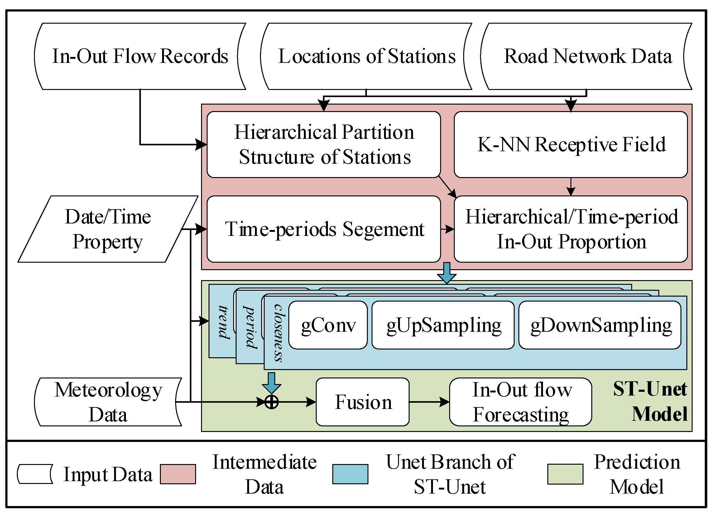
2.2. Framework
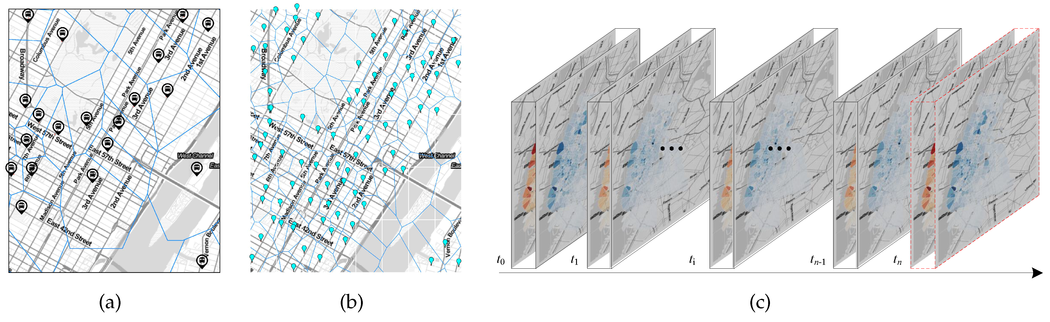
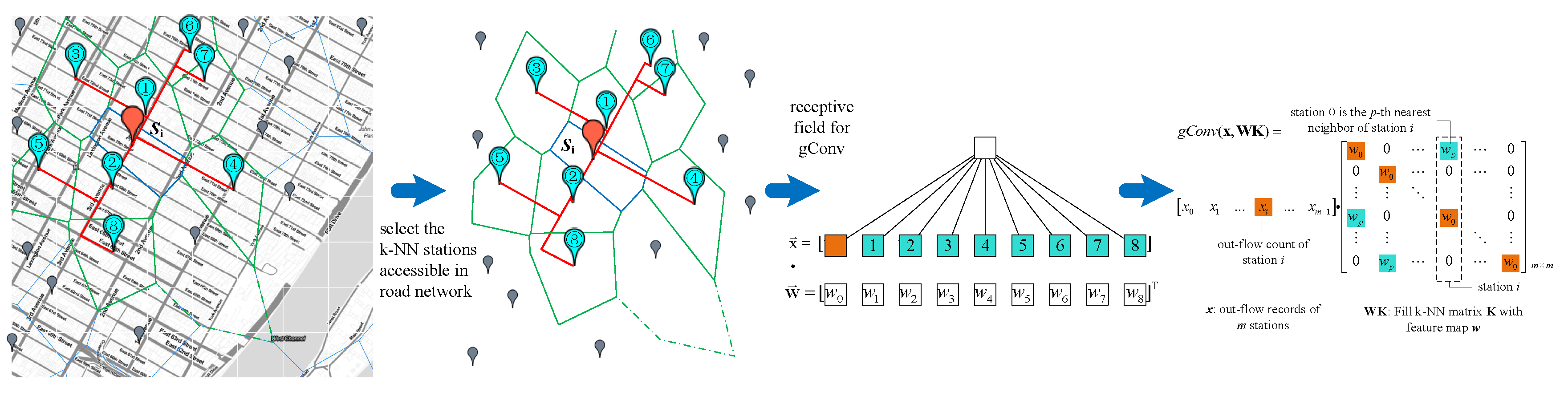
- k-NN (nearest neighbor) Receptive Field of Each Station. The receptive field of CNNs of each entry in regular grid data is its 8 or 24 neighbor grids (when using 3 × 3 or 5 × 5 feature maps, respectively). However, because the stations are scattered irregularly, the k-NN receptive field of each station should be redefined. Inspired by graph-CNNs utilizing graph labelings to impose an order on nodes [19], we define and figure out each station’s receptive field with its k ordered nearest neighbor stations reachable in the road network (See Section 3.3).
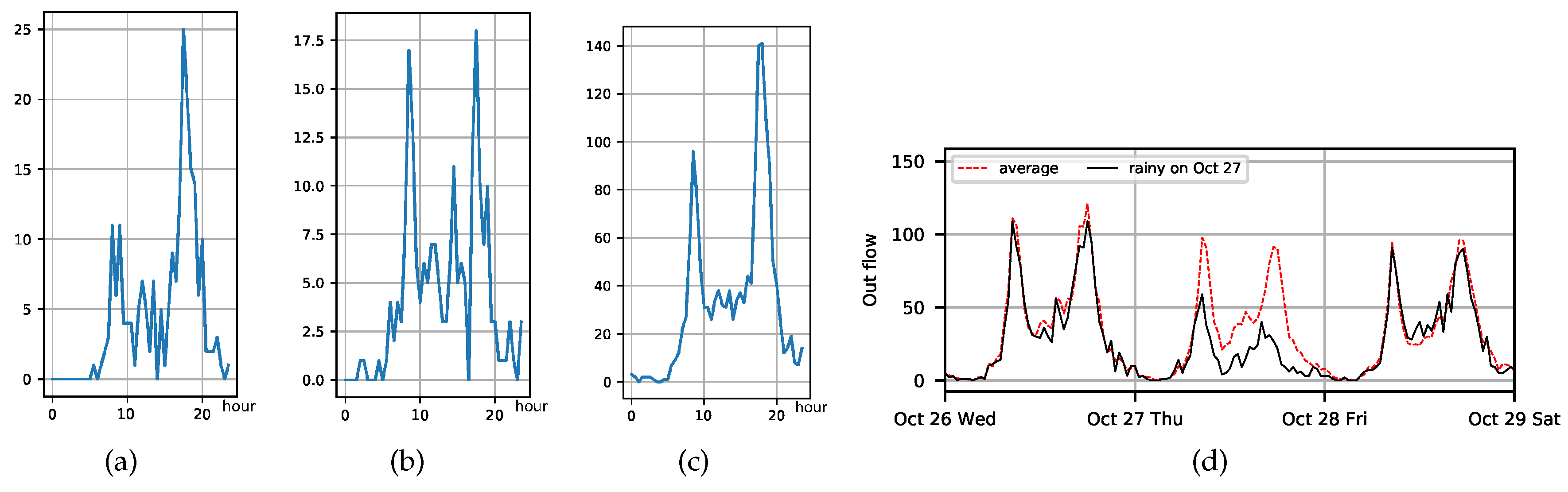
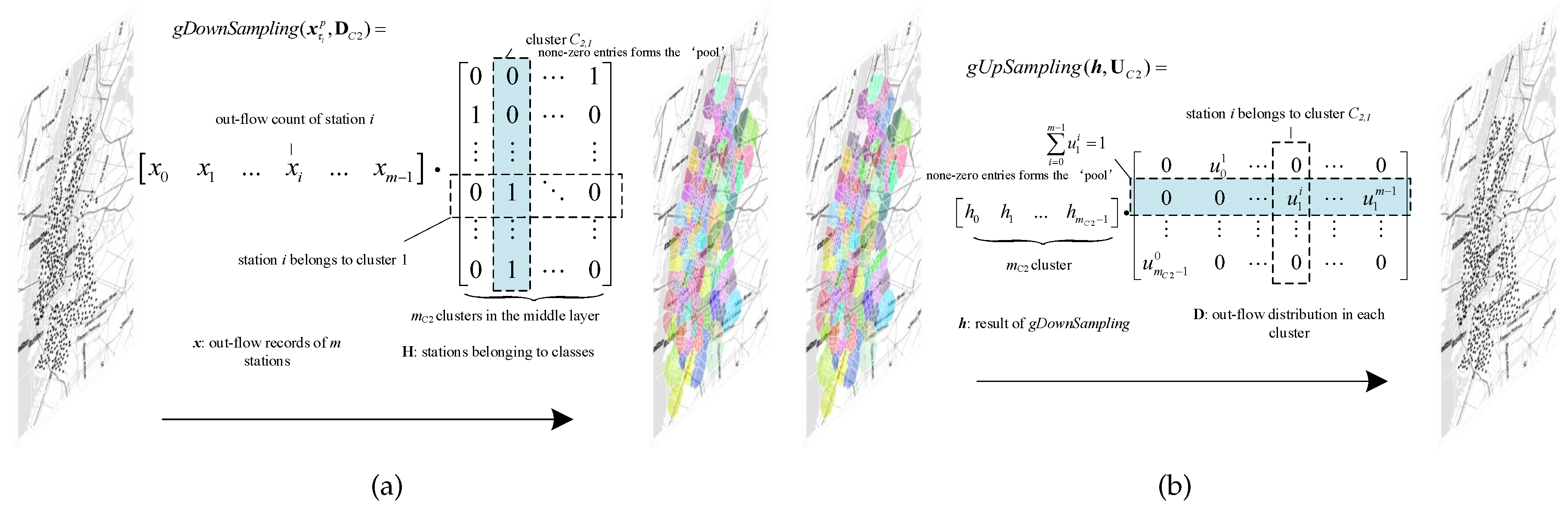
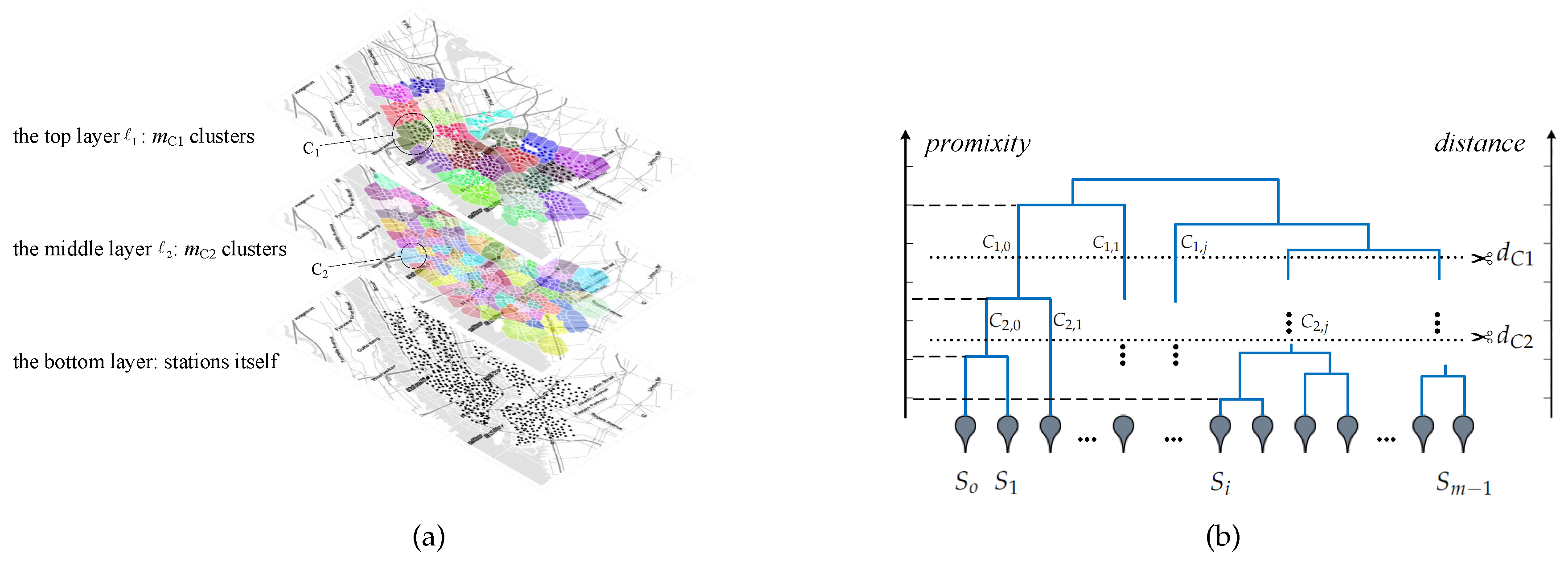
- Hierarchical Structure of Stations. From the view of one individual station, the changing regularity of in–out flow is difficult to determine because of its fluctuation, as shown in Figure 3a,b. However, it is much more robust and regular from the view of a region with several stations, as shown in Figure 3. Thus, we employ an agglomerative clustering algorithm to construct the hierarchical structure of the stations, which is based on the stations’ geo-locations and historical in–out flow data. This is used as auxiliary information to determine the ‘pools’ of downsampling/upsampling layers in ST-Unet, which enhance the forecasting stability (See Section 3.4).
- Time-periods Segmentation. Considering the temporal heterogeneity of crowd flow, we categorize according to seven time periods: 1. 7:00 a.m.–11:00 a.m. (morning rush hours); 2. 11:00 a.m.–4:00 p.m. (day hours); 3. 4:00 p.m.–9:00 p.m. (evening rush hours); and 4. 9:00 p.m.–7:00am (night hours); and 5. 0:00 a.m.–9:00 a.m. (night hours); 6. 9:00 a.m.–7:00 p.m. (trip hours); and 7. 7:00 p.m.–12:00 p.m. (evening hours) on weekends/holidays. Each time slot is labelled with a property field ‘’ indicating what kind of time periods it belongs to, i.e., .
- Hierarchical/Time-period In–Out proportion. According to the hierarchical structure of stations and different time periods, the maximum likelihood estimation method is used to estimate each station’s in–out flow proportion within its cluster. Such information is used to correct the up-sampling operation, replacing the usual adopted method—padding (See Section 3.4).
3. ST-Unet
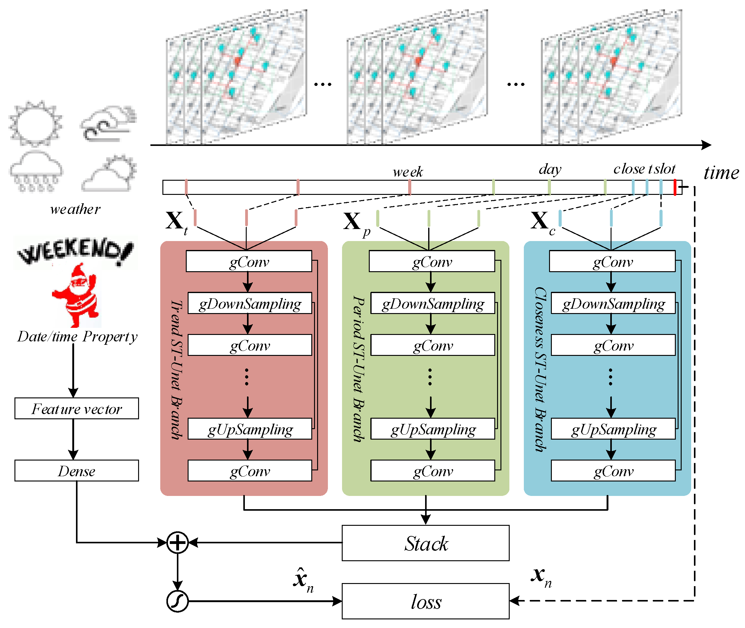
3.1. Overview
3.2. Unet Branch of ST-Unet
3.3. gConv
3.4. gDownSampling and gUpSampling
4. Experiments
4.1. Datasets
4.2. Hyperparameters Selection of ST-Unet
- Observing time unit : 30 min.
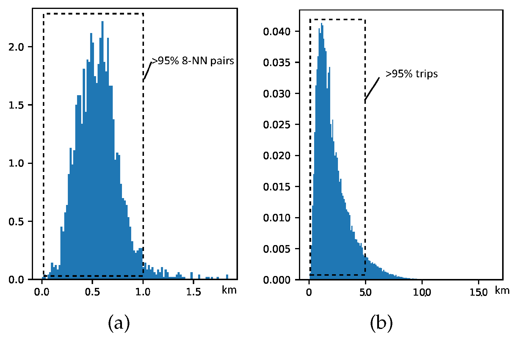
- k nearest neighbor stations: 4.
- The length l of time slots chosen to stack in the input of each Unet branch: 4.
- Constraints and to limit the size of each cluster of layer , : 2.5 km and 1.5 km (10.0 km and 5.0 km for Taxi dataset).
- , , in each Unet: 16, 16, 16.
- Activation function of gConv, gDownSampling, gUpSampling: relu.
- Loss function: as the metric MAE depicted in Section 4.3.
- Optimizer: Adam-optimizer [24].
- Terminated condition: The training reaches 400 iterations, or when the model does not achieve further improvement for 25 consecutive iterations on the validating data.
4.3. Baselines & Metric
- XGB: XGB, short for eXtreme Gradient Boosting, is an implementation of GBRT (gradient boosted decision trees) [25]. All input features are the same as ST-Unet.
- Ensemble: The ensembles of three predictive models proposed in Reference [13]: ARIMA, time-varying Poisson model, weighted time-varying Poisson model.
- VARIMA: Vector-ARIMA extends ARIMA to the multivariate case, which can capture the pairwise relations among the multi-time series.
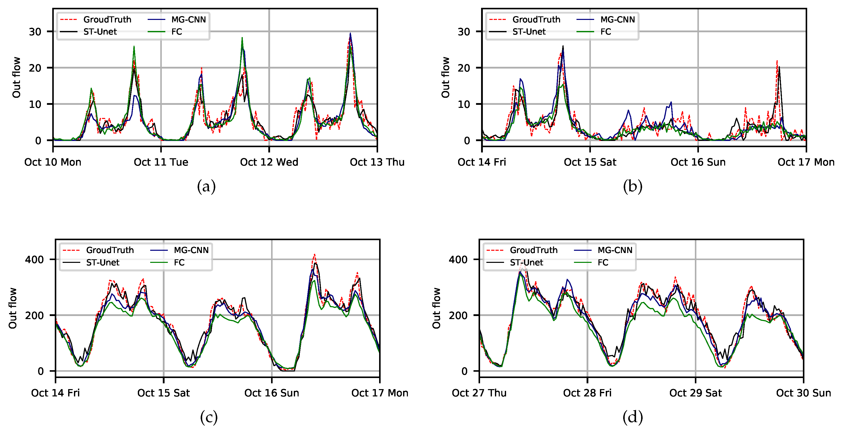
- FC: A three-layers of Full-Connected neural networks is built. Its output is the forecast of all stations’ in–out crowd flow. All input features are the same as ST-Unet.
- MG-CNN: Multi-graph convolutional networks, a deep neural network model with multiple graphs fusing CNNs for station-level future bike flow forecast [17]. The past six time slots history data are used to forecast the flow in the next time slot.
- Unet: Forecasting with only the closeness Unet branch (see Section 3.1).
- ST-net: Neither gDownSampling or gUpSampling are in the Unet branches, being replaced by gConv.
4.4. Results
5. Conclusions and Discussion
Author Contributions
Funding
Acknowledgments
Conflicts of Interest
Abbreviations
| SLCFF | Station-Level Crowd Flow Forecast |
| MSVR | Multi-output Support Vector Regression |
| ARIMA | Auto-Regressive Moving Average |
| VARIMA | Vector Auto-Regressive Integrated Moving Average |
| CNNs | Convolutional Neural Networks |
| LSTM | Long Short Term Memory neural networks |
References
- Hoang, M.X.; Zheng, Y.; Singh, A.K. FCCF: Forecasting citywide crowd flows based on big data. In Proceedings of the The ACM Sigspatial International Conference, Burlingame, CA, USA, 31 October–3 November 2016; pp. 1–10. [Google Scholar]
- Zhang, J.; Zheng, Y.; Qi, D. Deep Spatio-Temporal Residual Networks for Citywide Crowd Flows Prediction. In Proceedings of the Thirty-First AAAI Conference on Artificial Intelligence, San Francisco, CA, USA, 4–10 February 2017; pp. 1655–1661. [Google Scholar]
- Alexander, L.; Jiang, S.; Murga, M.; González, M.C. Origin–destination trips by purpose and time of day inferred from mobile phone data. Transp. Res. Part C Emerg. Technol. 2015, 58, 240–250. [Google Scholar] [CrossRef]
- Scholz, R.W.; Lu, Y. Detection of dynamic activity patterns at a collective level from large-volume trajectory data. Int. J. Geogr. Inf. Sci. 2014, 28, 946–963. [Google Scholar] [CrossRef]
- Kung, K.S.; Greco, K.; Sobolevsky, S.; Ratti, C. Exploring universal patterns in human home-work commuting from mobile phone data. PLoS ONE 2014, 9, e96180. [Google Scholar] [CrossRef] [PubMed]
- Zheng, K.; Zheng, Y.; Yuan, N.J.; Shang, S.; Zhou, X. Online discovery of gathering patterns over trajectories. IEEE Trans. Knowl. Data Eng. 2014, 26, 1974–1988. [Google Scholar] [CrossRef]
- Borchani, H.; Varando, G.; Bielza, C.; Larrañaga, P. A survey on multi-output regression. Wiley Interdiscip. Rev. Data Min. Knowl. Discov. 2015, 5, 216–233. [Google Scholar] [CrossRef]
- Cheng, X.; Ren, L.; Cui, J.; Zhang, Z. Traffic Flow Prediction with Improved SOPIO-SVR Algorithm. In Proceedings of the Monterey Workshop on Challenges and Opportunity with Big Data, Beijing, China, 8–11 October 2016; pp. 184–197. [Google Scholar]
- Feng, S.; Hao, C.; Du, C.; Li, J.; Ning, J. A Hierarchical Demand Prediction Method with Station Clustering for Bike Sharing System. In Proceedings of the IEEE Third International Conference on Data Science in Cyberspace, Guangzhou, China, 18–21 June 2018. [Google Scholar]
- Hong, W.C.; Dong, Y.; Zheng, F.; Lai, C.Y. Forecasting urban traffic flow by SVR with continuous ACO. Appl. Math. Model. 2011, 35, 1282–1291. [Google Scholar] [CrossRef]
- Liu, J.; Sun, L.; Li, Q.; Ming, J.; Liu, Y.; Xiong, H. Functional zone based hierarchical demand prediction for bike system expansion. In Proceedings of the 23rd ACM SIGKDD International Conference on Knowledge Discovery and Data Mining, Halifax, NS, Canada, 13–17 August 2017; pp. 957–966. [Google Scholar]
- Li, Y.; Zheng, Y.; Zhang, H.; Chen, L. Traffic prediction in a bike-sharing system. In Proceedings of the 23rd SIGSPATIAL International Conference on Advances in Geographic Information Systems, Seattle, WA, USA, 3–6 November 2015; p. 33. [Google Scholar]
- Moreira-Matias, L.; Gama, J.; Ferreira, M.; Mendes-Moreira, J.; Damas, L. Predicting taxi—Passenger demand using streaming data. IEEE Trans. Intell. Transp. Syst. 2013, 14, 1393–1402. [Google Scholar] [CrossRef]
- Zhan, X.; Zheng, Y.; Yi, X.; Ukkusuri, S.V. Citywide traffic volume estimation using trajectory data. IEEE Trans. Knowl. Data Eng. 2017, 272–285. [Google Scholar] [CrossRef]
- Min, W.; Wynter, L. Real-time road traffic prediction with spatio-temporal correlations. Transp. Res. Part C Emerg. Technol. 2011, 19, 606–616. [Google Scholar] [CrossRef]
- Asif, M.T.; Dauwels, J.; Goh, C.Y.; Oran, A.; Fathi, E.; Xu, M.; Dhanya, M.M.; Mitrovic, N.; Jaillet, P. Unsupervised learning based performance analysis of n-support vector regression for speed prediction of a large road network. In Proceedings of the 15th International IEEE Conference on the IEEE Intelligent Transportation Systems (ITSC), Anchorage, AK, USA, 16–19 September 2012; pp. 983–988. [Google Scholar]
- Chai, D.; Wang, L.; Yang, Q. Bike flow prediction with multi-graph convolutional networks. In Proceedings of the 26th ACM SIGSPATIAL International Conference on Advances in Geographic Information Systems (ACM), Seattle, WA, USA, 6–9 November 2018; pp. 397–400. [Google Scholar]
- Tian, Y.; Pan, L. Predicting short-term traffic flow by long short-term memory recurrent neural network. In Proceedings of the IEEE International Conference on Smart City/SocialCom/SustainCom (SmartCity), Chengdu, China, 19–21 December 2015; pp. 153–158. [Google Scholar]
- Niepert, M.; Ahmed, M.; Kutzkov, K. Learning convolutional neural networks for graphs. In Proceedings of the International Conference on Machine Learning, New York, NY, USA, 17 May 2016; pp. 2014–2023. [Google Scholar]
- Ronneberger, O.; Fischer, P.; Brox, T. U-net: Convolutional networks for biomedical image segmentation. In Proceedings of the International Conference on Medical Image Computing and Computer-Assisted Intervention, Munich, Germany, 5–9 October 2015; pp. 234–241. [Google Scholar]
- Tobler, W.R. A computer movie simulating urban growth in the Detroit region. Econ. Geogr. 1970, 46, 234–240. [Google Scholar] [CrossRef]
- Defferrard, M.; Bresson, X.; Vandergheynst, P. Convolutional neural networks on graphs with fast localized spectral filtering. In Proceedings of the Advances in Neural Information Processing Systems, Barcelona, Spain, 5–10 December 2016; pp. 3844–3852. [Google Scholar]
- Berkhin, P. A survey of clustering data mining techniques. In Grouping Multidimensional Data; Springer: Berlin/Heidelberg, Germany, 2006; pp. 25–71. [Google Scholar]
- Kingma, D.P.; Ba, J. Adam: A method for stochastic optimization. arXiv, 2014; arXiv:1412.6980. [Google Scholar]
- Chen, T.; Guestrin, C. Xgboost: A scalable tree boosting system. In Proceedings of the 22nd ACM Sigkdd International Conference on Knowledge Discovery and Data Mining, San Francisco, CA, USA, 13–17 August 2016; pp. 785–794. [Google Scholar]


| Data Source | Citi | DC | Divvy | Taxi |
|---|---|---|---|---|
| Time Span | 1 April–30 October, 2016 | 1 April–30 October, 2017 | ||
| Stations | 572 | 367 | 469 | 263 * |
| Records | 9,796,166 | 2,343,044 | 2,853,665 | 65,235,951 |
| Cities | Rainy Dates | Foggy Dates |
|---|---|---|
| NYC | 21/10/2016, 27/10/2016, 29/10/2017 | 21/10/2016, 27/10/2016, 30/10/2016, 29/10/2017 |
| Chicago | 16/10/2016 | 26/10/2016, 27/10/2016 |
| DC | - | 12/10/2016, 13/10/2016, 17/10/2016 |
| Dataset | Methods | XGB | Ensemble | VARIMA | FC | MG-CNN | Unet | ST-net | ST-Unet |
|---|---|---|---|---|---|---|---|---|---|
| CITI | whole | 1.057 | 1.067 | 1.247 | 1.077 | 1.023 | 1.028 | 1.103 | 0.98 |
| workday | 1.088 | 1.044 | 1.301 | 1.126 | 1.074 | 1.061 | 1.145 | 1.019 | |
| weekend | 0.979 | 1.125 | 1.112 | 0.955 | 0.896 | 0.946 | 0.998 | 0.883 | |
| holiday | 1.072 | 1.07 | 1.279 | 1.097 | 1.006 | 1.101 | 1.14 | 1.046 | |
| rainy | 0.98 | 1.111 | 0.86 | 0.974 | 0.918 | 0.841 | 0.897 | 0.822 | |
| foggy | 0.988 | 1.103 | 0.913 | 0.93 | 0.926 | 0.887 | 0.932 | 0.843 | |
| DC | whole | 0.489 | 0.519 | 0.46 | 0.497 | 0.501 | 0.493 | 0.472 | 0.425 |
| workday | 0.481 | 0.479 | 0.451 | 0.487 | 0.494 | 0.493 | 0.471 | 0.428 | |
| weekend | 0.509 | 0.619 | 0.483 | 0.522 | 0.519 | 0.493 | 0.475 | 0.418 | |
| holiday | 0.515 | 0.487 | 0.471 | 0.48 | 0.505 | 0.498 | 0.479 | 0.419 | |
| rainy | - | - | - | - | - | - | - | - | |
| foggy | 0.499 | 0.468 | 0.48 | 0.512 | 0.49 | 0.502 | 0.482 | 0.443 | |
| DIVVY | whole | 0.442 | 0.448 | 0.417 | 0.404 | 0.422 | 0.442 | 0.489 | 0.39 |
| workday | 0.439 | 0.43 | 0.412 | 0.401 | 0.411 | 0.43 | 0.475 | 0.392 | |
| weekend | 0.45 | 0.493 | 0.43 | 0.412 | 0.45 | 0.472 | 0.524 | 0.385 | |
| holiday | 0.514 | 0.533 | 0.494 | 0.488 | 0.524 | 0.545 | 0.644 | 0.517 | |
| rainy | 0.43 | 0.438 | 0.4 | 0.387 | 0.433 | 0.426 | 0.399 | 0.364 | |
| foggy | 0.342 | 0.324 | 0.284 | 0.298 | 0.321 | 0.335 | 0.318 | 0.285 | |
| TAXI | whole | 3.552 | 3.786 | 4.372 | 4.601 | 3.642 | 3.731 | 3.422 | 3.23 |
| workday | 3.463 | 3.478 | 4.287 | 4.54 | 3.463 | 3.613 | 3.37 | 3.142 | |
| weekend | 3.775 | 4.556 | 4.585 | 4.754 | 4.09 | 4.026 | 3.552 | 3.45 | |
| holiday | - | - | - | - | - | - | - | - | |
| rainy | 4.411 | 4.599 | 4.29 | 4.684 | 4.438 | 4.348 | 4.081 | 4.043 | |
| foggy | 4.411 | 4.599 | 4.29 | 4.684 | 4.438 | 4.348 | 4.081 | 4.043 |
© 2019 by the authors. Licensee MDPI, Basel, Switzerland. This article is an open access article distributed under the terms and conditions of the Creative Commons Attribution (CC BY) license (http://creativecommons.org/licenses/by/4.0/).
Share and Cite
Zhou, Y.; Chen, H.; Li, J.; Wu, Y.; Wu, J.; Chen, L. Large-Scale Station-Level Crowd Flow Forecast with ST-Unet. ISPRS Int. J. Geo-Inf. 2019, 8, 140. https://doi.org/10.3390/ijgi8030140
Zhou Y, Chen H, Li J, Wu Y, Wu J, Chen L. Large-Scale Station-Level Crowd Flow Forecast with ST-Unet. ISPRS International Journal of Geo-Information. 2019; 8(3):140. https://doi.org/10.3390/ijgi8030140
Chicago/Turabian StyleZhou, Yirong, Hao Chen, Jun Li, Ye Wu, Jiangjiang Wu, and Luo Chen. 2019. "Large-Scale Station-Level Crowd Flow Forecast with ST-Unet" ISPRS International Journal of Geo-Information 8, no. 3: 140. https://doi.org/10.3390/ijgi8030140
APA StyleZhou, Y., Chen, H., Li, J., Wu, Y., Wu, J., & Chen, L. (2019). Large-Scale Station-Level Crowd Flow Forecast with ST-Unet. ISPRS International Journal of Geo-Information, 8(3), 140. https://doi.org/10.3390/ijgi8030140