An Urban Road-Traffic Commuting Dynamics Study Based on Hotspot Clustering and a New Proposed Urban Commuting Electrostatics Model

Abstract

With the recent rapid development of cities, the dynamics of urban road-traffic commuting are becoming more and more complex. In this research, we study urban road-traffic commuting dynamics based on clustering analysis and a new proposed urban commuting electrostatics model. As a case study, we investigate the characteristics of urban road-traffic commuting dynamics during the morning rush hour in Beijing, China, using over 1.3 million Global Positioning System (GPS) data records of vehicle trajectories. The hotspot clusters are identified using clustering analysis, after which the urban commuting electric field is simulated based on an urban commuting electrostatics model. The results show that the areas with high electric field intensity tend to have slow traffic, and also that the vehicles in most areas tend to head in the same direction as the electric field. The results above verify the validity of the model, in that the electric field intensity can reflect the traffic pressure of an area, and that the direction of the electric field can reflect the traffic direction in that area. This new proposed urban commuting electrostatics model helps greatly in understanding urban road-traffic commuting dynamics and has broad applicability for the optimization of urban and traffic system planning.

1. Introduction

Urban agglomerations are the result of societal and economic development around the world, and of globalization, regional urbanization, integrated regional economies, and well-developed traffic networks [1]. In May 2016, the journal Science published a series of articles entitled “Rise of The Urban Planet”, in which the authors asserted that over half of the world’s population live in cities, and that this proportion would reach two-thirds by 2050 [2]. In this context, large-scale urban commuting arises due to urban population migration and the development of urban transportation, and such commuting has quickly become a popular research topic. Urban commuting analysis is a type of spatial analysis which seeks to explain patterns of human mobility and its spatial expression in terms of mathematics and geometry [3]. Urban commuting analysis is of great importance, since urban commuting is intimately related to the social environment and urban development [4]. Characterizing and extracting information about urban commuting has been one of the main goals of urban commuting studies. The study of urban commuting currently draws attention from several fields of research, such as urban function planning [5], rural–urban differences [6], the construction environment [7], population distribution [8], traffic states estimation [9], commuting tools, time, cost and distance [10,11], travel patterns [12], public behavior [13], road incident impact evaluation [14] and node ranking of urban networks [15].

Data for urban commuting analysis have become increasingly abundant and diverse. Besides conventional aggregate data, such as censuses, community surveys and questionnaires, the appearance of new technologies offers more types of data about cities. These data are provided by sensors, public or private services, mobile devices, web services, social networks, location-based services and GPS trajectories [16,17]. For instance, Agryzkov et al. compared the data extracted from a social network with data collected from the fieldwork in order to establish the appropriateness of understanding the activity that takes place in Murcia, Spain [16]. Wan et al. tried to simulate traffic commuting patterns in Beijing, China, based on a theory of spatial equilibrium using location-based service (LBS) data [18]. Furthermore, Misra introduced the concept of socio-physical analytics which fused transportation-related data across multiple modalities with social media sensing to identify and characterize urban micro-events [19]. Among all these data, data from GPS trajectories have the characteristics of large sample size, high data density, wide coverage, and high accuracy [20]. Therefore, research on urban commuting using GPS trajectories has been extensively conducted in recent years. For instance, Fu et al. investigated commuting behavior by taxi and studied the spatiotemporal distribution characteristics of urban residents’ travel activities, based on vehicle trajectory data generated by taxi GPS devices [21]. Mao et al. tried to identify potentially meaningful places by using the spatial clustering of taxi Origin-Destination (O-D), identifying threshold values from statistics of the O-D clusters, and then extracting urban jobs housing structures, in order to understand the spatial distribution and temporal trends of the revealed urban structures and implied household commuting behavior [22]. In summary, regarding the study of urban commuting analysis, previous studies mainly focused on and contributed much to detecting urban commuting events and profiling urban commuting characteristics, including the characteristics of commuting generations and the characteristics of commuting dynamics. As a result, in recent years, O-D patterns, the distribution of hotspots, and the distribution of congested segments have been subjected to abundant research based on different methods in recent years.

However, despite plentiful research on urban commuting analysis, insufficient attention has been paid to studying the correlation between urban commuting generations and commuting dynamics, and moreover there are still no effective tools to handle this problem in practice. Some researchers have tried to identify a connection between trip patterns and origins/destinations. For instance, an approach was suggested to synthesize trips and catchment areas between towns in a region based on the gravity model, which introduced an analogy with the law of gravitation to urban commuting analysis [23]. In another study, long-distance communications were characterized by a gravity model, and the authors found that the intensity of communication between two cities was proportional to the products of the two populations divided by the square of the distance between the cities [24]. However, the studies mentioned above estimated urban commuting trips based on the static population data of the towns, instead of directly using the observed trip pattern or dynamical O-D trajectories, which makes the results rough and imprecise [25]. In brief, new methods are needed for the in-depth study of the correlation between urban commuting generations and commuting dynamics. This need motivated the present study. The main objectives of this study were to analyze the characteristics of commuting generations and the characteristics of commuting dynamics separately, and to clarify the correlation between them. In particular, we achieved this purpose by establishing a set of simple, universal, and effective methods, which is also the main contribution of this study.

In this study, clustering analysis based on an O-D hotspot clustering model was first implemented to profile the O-D hotspots in the morning rush hour in Beijing, China. An urban commuting electrostatics model was proposed based on the results of the clustering analysis, and an urban commuting electric field was built in two-dimensional urban space. Next, we chose features of moving vehicles as the characteristics of urban commuting dynamics and clustered the features of vehicles to the same two-dimensional urban space. This allowed the further analysis on the correlation between urban commuting generations and commuting dynamics. The remainder of this paper is organized as follows: Section 2 introduces the method design of this study, including the clustering method and urban commuting electrostatics model; Section 3 presents the study area and details of the taxi trajectory data used in the study; Section 4 reports and discusses the results; and Section 5 concludes the paper with a summary of the main findings.

2. Methodology

The methodology used in this study is consisted by two parts, as shown in Figure 1. First, a clustering analysis was conducted using geographic data and GPS data of vehicle trajectories to profile the pick-up and drop-off hotspot clusters. The practical meaning of hotspot clusters is the areas/zones with concentrated pick-up or drop-off events in a city during a specific period of time. Second, an urban commuting electric field was built based on the urban commuting electrostatics model, using GPS data of vehicle trajectories and the distribution of hotspot clusters. The key connection between the clustering analysis and the urban commuting electrostatics model is the pick-up and drop-off hotspot clusters. The hotspot clusters are the output of the first method and are simultaneously the input for the second model.

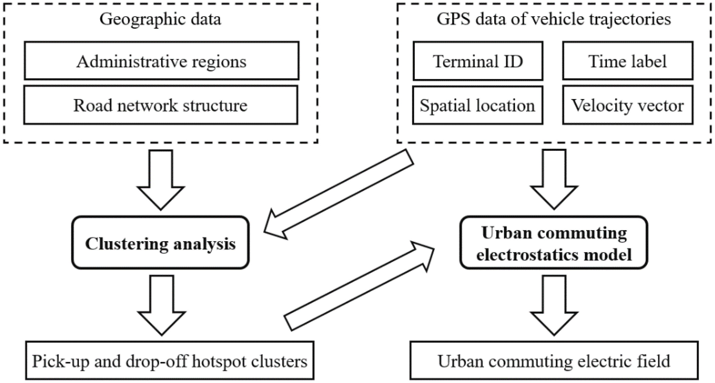
2.1. Origin-Destination (O-D) Hotspot Clustering Model

O-D travel demand is critical information for planning, operating, and analyzing a transportation system in a city [26]. The O-D scattered points in megacities such as Beijing are very dense, even for a short time period, and particularly during rush hour. It takes immense manpower and time to study the huge volume of O-D lines individually. Clustering is an effective method to simplify data processing and hence simplify the problem [27]. The O-D points can be clustered into pick-up clusters or drop-off clusters, and then the O-D lines among these clusters can be studied. Clustering methods can be classified into five main categories: (1) hierarchical methods; (2) partition-based methods; (3) density-based methods; (4) grid-based methods; and (5) model-based methods [27,28,29,30,31]. The K-means algorithm is a widely used partition-based clustering method [32]. The value of the parameter K needs to be artificially set before the clustering process begins and cannot be changed during the process. The classical K-means algorithm is not suitable for O-D hotspot clustering since it is usually difficult to appropriately estimate the number of O-D hotspot clusters for a city. The Iterative Self Organizing Data Analysis Techniques Algorithm (ISODATA) is more suitable for studying the problem, as the cluster number in ISODATA is not decided in advance, which makes the model different from the K-means algorithm. The core idea of ISODATA is very intuitive: when the distance between two cluster centers is less than a threshold, the two clusters will be merged into a single cluster. When the standard deviation of a cluster is greater than a certain threshold, or the number of samples exceeds a certain threshold, this cluster will be split into two clusters. When the number of samples in a cluster is less than a certain threshold, the cluster will be deleted [33,34]. Previously, we proposed an O-D hotspot clustering model based on ISODATA [35]. The parameters of this model are shown in

Table 1. The parameters of the proposed Origin-Destination (O-D) hotspot clustering model.

Parameter	Meaning
$K$	Prospective number of clustering centers in the model
$N_c$	Number of initial clustering centers
$L$	Number of groups that could be merged into one merging step
$I$	Number of iterations in the iteration operation
$S_j$	Collection mark of the clusters, $j=1,2,\dots ,N_C$
$N_j$	Number of samples in the cluster $S_j$, $j=1,2,\dots ,N_C$
${\theta }_N$	Minimum number of samples in a clustering center; the clustering center will be deleted if the number of samples is less than ${\theta }_N$
${\theta }_S$	Standard deviation of the distribution of the between-sample distance in a clustering center
${\theta }_C$	Minimum distance between two clustering centers; the clustering centers will be merged if the distance between them is less than ${\theta }_C$

.

There are several steps in the proposed O-D hotspot clustering model [36].

Normal K-means Step: In this step, $N$ samples are classified into different clusters. This step contains five sub-steps:

(1) Suppose there are initially $N$ samples in a system, sort them into different $S_j, j=1,2,\dots ,N_C$. The samples are denoted by $\{x_1, x_2,\dots ,x_N\}$. Preselect $N_C$ initial clustering centers discretionarily, denoted by $\{z_1,z_2,\dots ,z_{N_C}\}$. The distance between a sample and the clustering center $z_j$ is denoted by $D_j$. If $D_j = \min \{\Vert x-z_j\Vert ,j=1,2,\dots ,N_C\}$, which means $\Vert x-z_j\Vert$ is minimum for all the distances of a sample to the clustering centers, then $x\in S_j$;

(2) If the number of samples in $S_j$ is less than ${\theta }_N$, then delete the cluster, $N_C=N_C-1$. Go to Step 1 and reclassify $N$ samples into different $S_j, j=1,2,\dots ,N_C$;

(3) Revise the clustering centers:

$$z_j=\frac{1}{N_j}{\displaystyle \sum }_{x\in S_j}x, j=1,2,\dots ,N_C$$

(1)

(4) Calculate the mean distance of the samples in a cluster to the clustering center:

$$\overline{D_j}=\frac{1}{N_j}{\displaystyle \sum }_{x\in S_j}\Vert x-z_j\Vert , j=1,2,\dots ,N_C$$

(2)

(5) Calculate the total mean distance of all the samples to their corresponding clustering centers:

$$\overline{D}= \frac{1}{N}{\displaystyle \sum }_{j=1}^N{N}_j\overline{D_j}$$

(3)

Dividing Step: If $N_C\le \frac{K}{2}$ or ($i\%2==0 \mathrm{and} N_C<2K$), the program enters a dividing step, which contains two sub-steps:

(1) Calculate the vector of the standard deviation of each cluster. In the following equations, $i$ denotes the dimension of the eigenvector of samples while $j$ denotes the number of clusters. The maximum component in ${\sigma }_j$ is denoted by ${\sigma }_{jmax}$:

$${\sigma }_j={\left({\sigma }_{1j},{\sigma }_{2j},\dots ,{\sigma }_{nj}\right)}^T, j=1,2,\dots ,N_C$$

(4)

$${\sigma }_{ij}=\sqrt{\frac{1}{N_j}{\displaystyle \sum }_{k=1}^{N_j}{\left(x_{ik}-z_{ij}\right)}^2}, i=1,2,\dots ,n, j=1,2,\dots ,N_C$$

(5)

(2) If any ${\sigma }_{jmax}$ in the collection $\{{\sigma }_{jmax},j=1,2,\dots ,N_c\}$ satisfies ${\sigma }_{jmax}>{\theta }_S$ and (($\overline{D_j}>\overline{D}$ and $N_j>2\left({\theta }_N+1\right)$) or $N_C\le \frac{K}{2}$), divide $S_j$ into two clusters. $N_c=N_c+1$.

Merging Step: If $N_C\ge 2K$ or $i\%2==0$, the program enters a merging step, which contains two sub-steps:

(1) Calculate the distances of different clustering centers:

$$D_{ij}=\Vert z_i-z_j\Vert , i=1,\dots ,N_C-1, j=i+1,\dots ,N_C$$

(6)

(2) Compare the values of $D_{ij}$ and ${\theta }_C$. If $D_{ij}$ is less than ${\theta }_C$, put these $D_{ij}$ into a set and sort them from small to large as $\{D_{i_1}{D}_{j_1},D_{i_2}{D}_{j_2}, \dots ,D_{i_L}{D}_{j_L}\}$. Notice that $L$ is the number of groups that could be merged in one merging step. Merge these clustering centers and obtain a new clustering center.

$$z_k^{*}=\frac{1}{N_{i_k}+N_{j_k}}\left[N_{i_k}·z_{i_k}+N_{j_k}·z_{j_k}\right],k=1,\dots ,L$$

(7)

2.2. Classical Theory of Electrostatics

Coulomb’s law states that oppositely charged particles attract each other while particles with the same charge repel each other with a force that is proportional to the magnitude of each charge and inversely proportional to the square of the distance between the particles, the force being directed along the line joining the particles. If “1” and “2” are two particles with charges $q_1$ and $q_2$, respectively, and are separated by a distance $r_{12}$, the electric force exerted by “1” and “2” as given by Coulomb’s law is:

$$F_{12}=K·\frac{q_1{q}_2}{{r_{12}}^2}=-F_{21},$$

(8)

where $K$ is the constant of proportionality and $F_{12}$ is the force exerted by “2” on “1”. In vector notation, this equation can be written as:

$$\overrightarrow{F_{12}}=K·\frac{q_1{q}_2}{|r_{12}{|}^2}·\widehat{e_r}=K·\frac{q_1{q}_2}{|r_{12}{|}^3}·\overrightarrow{r_{12}},$$

(9)

where $\widehat{e_r}=\overrightarrow{r_{12}}/\left|r_{12}\right|$ is the unit vector along $\overrightarrow{r_{12}}$.

If there are more than two particles with charges, the total force on one particle is the vector sum of the forces it experiences due to all other particles separately; this is known as the principle of superposition. If there are three particles, denoted by “1”, “2”, and “3”, the force on $q_3$ is given by:

$$\overrightarrow{F}=\overrightarrow{F_{13}}+\overrightarrow{F_{23}}=K·\frac{q_1{q}_3}{|r_{13}{|}^3}·\overrightarrow{r_{13}}+K·\frac{q_2{q}_3}{|r_{23}{|}^3}·\overrightarrow{r_{23}}$$

(10)

The force acting on a charge $q_j$ due to a number of other charges is:

$$\overrightarrow{F_{j }}=K{\displaystyle \sum }_{i\ne j}\frac{q_i{q}_j}{|r_{ij}{|}^3}\overrightarrow{r_{ij}}$$

(11)

The electric field at a point $P$ is defined by:

$$\overrightarrow{E\left(r_0\right)}=K\sum \frac{q_i}{{\left|r_0-r_i\right|}^3}\left(\overrightarrow{r_0}-\overrightarrow{r_i}\right),$$

(12)

where $\overrightarrow{r_0}$ is the location vector of the point $P$, and $\overrightarrow{r_i}$ are the location vectors giving the location of the other charges. The strength of the field $\left|E\left(r\right)\right|$ is called the electric field intensity. If a charge $q$ is placed at a point at which the field is $\overrightarrow{E}$, the force acting on the charge is:

$$\overrightarrow{F}=q\overrightarrow{E}$$

(13)

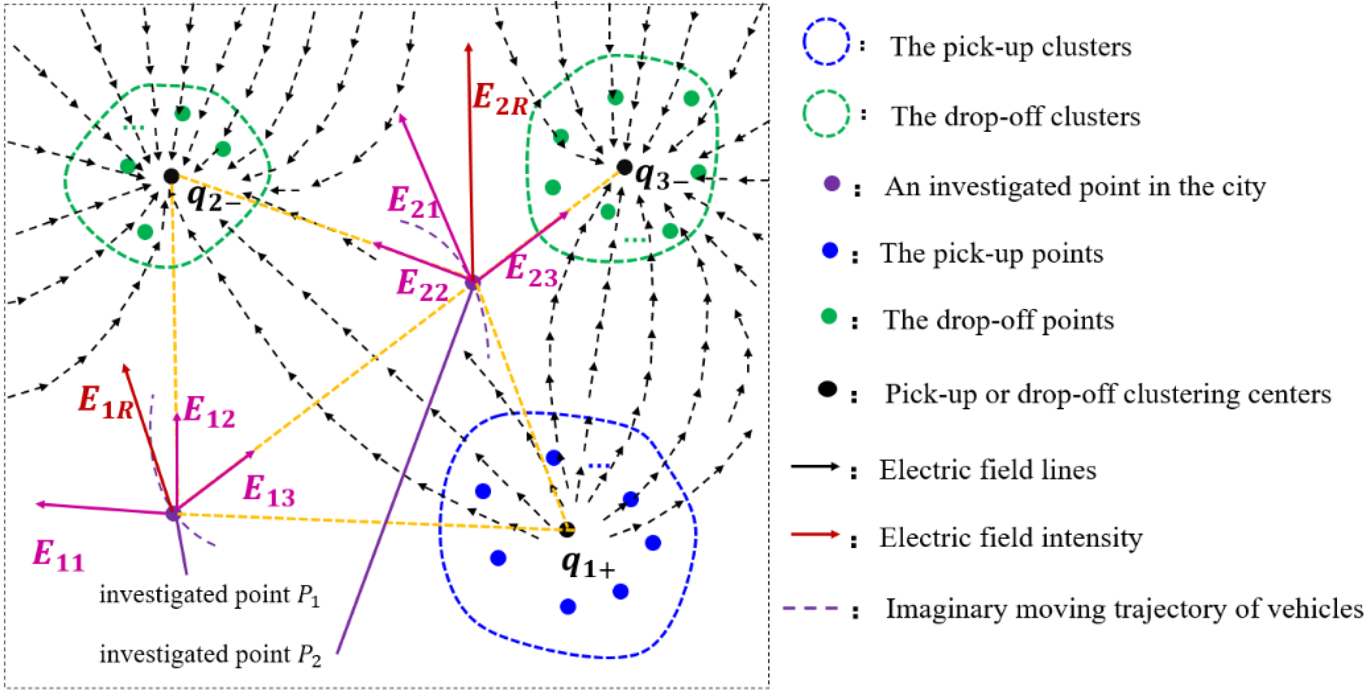
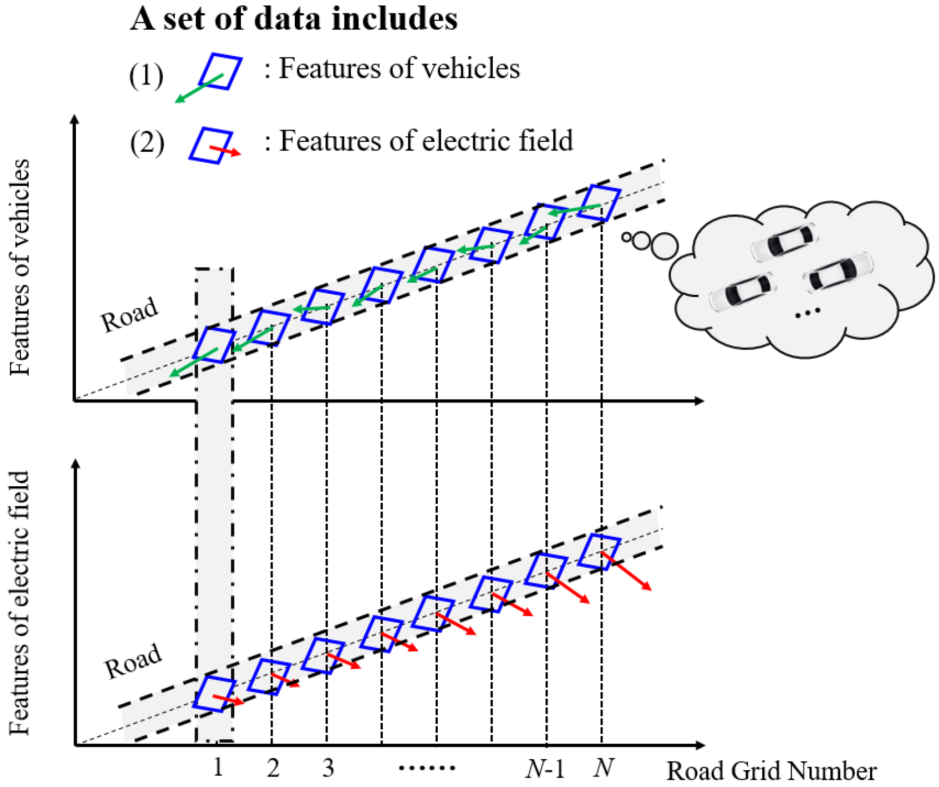
2.3. Urban Commuting Electrostatics Model

There are a large number of spatial migration patterns for people in cities. For example, the patterns of home–work–home, home–education–home, and home–driving children to school-work-picking up children from school-home pattern are especially common [37]. No matter what the spatial migration patterns are, people’s trajectories can be considered to be an O-D line or can be cut into several O-D lines. These O-D lines start from the pick-up origins and end at the drop-off destinations. The spatial migration of people via vehicles can be considered to be the outcome of a repulsion force from the pick-up origin and an attraction force from the drop-off destination. Based on this analogy, a new urban commuting electrostatics model is proposed which analogizes the driving force of people’s migration to the force acting on a charge in an electric field.

In the model, people are considered to be positive charges. With this assumption, the pick-up origins are considered to be static positive charges and the drop-off origins are considered to be static negative charges. Studying the repulsion forces, the attraction forces, and the corresponding spatial migration of people will help to better understand the principle of urban road-traffic commuting. However, it is difficult to directly study people’s trajectories one by one due to the huge amounts of data involved. In this paper, road points are chosen as the study objects. For a specific road point, we can find that there are various vehicles with totally different O-D lines passing through the point. These vehicles are influenced by different pick-up hotspot clusters and drop-off hotspot clusters. From the perspective of big data, the commuting features of the road points in a city are influenced by all the pick-up hotspot clusters and drop-off hotspot clusters. An urban commuting electric field is formed in the city based on the model, despite the fact that the forces on a single vehicle are only exerted by its own pick-up point and drop-off point.

To simplify the problem, we consider that the magnitude of charges is concentrated in the clustering center of each cluster. A diagrammatic view of the urban commuting electrostatics model is shown in Figure 2.

Suppose that there are $N$ pick-up and drop-off hotspot clusters and $M$ road points. The urban commuting electric field can be calculated by Equation (14):

$$\overrightarrow{E\left(r_{ji}\right)}=\{\begin{array}{c}K{\displaystyle \sum _{i=1}^N}\frac{q_i}{{\left|r_j-r_i\right|}^3}·\left(\overrightarrow{r_j}-\overrightarrow{r_i}\right), if \left|r_j-r_i\right|>\Gamma \hfill \\ K{\displaystyle \sum _{i=1}^N}\frac{q_i}{{\Gamma }^2·\left|r_j-r_i\right|}·\left(\overrightarrow{r_j}-\overrightarrow{r_i}\right), if \left|r_j-r_i\right|\le \Gamma \hfill \end{array},i = 1,2,\dots ,N, j=1,2,\dots ,M,$$

(14)

$$\overrightarrow{E\left(r_j\right)}={\displaystyle \sum }_{i=1}^N\overrightarrow{E\left(r_{ji}\right)}, i=1,2,\dots ,N, j=1,2,\dots ,M,$$

(15)

where $\overrightarrow{r_j}$ is the location vector of the road point $j$; $\overrightarrow{r_i}$ are the location vectors giving the location of the pick-up or drop-off hotspot clustering centers; $q_i$ is the charge of cluster $i$, and represents the number of people getting into or getting out of vehicles during the study period. Thus, the unit of $q_i$ is “person”; $K$ is the unit conversion coefficient, and can be set to be 1 m²/person in the SI system of units; and $\Gamma$ is an artificially set boundary value of the distance between a road point and a clustering center. If the road points are too close to a specific clustering center, the electric field intensity $\left|\overrightarrow{E\left(r_{ji}\right)}\right|$ contributed by the clustering center will be too large. The value of $\Gamma$ was set as one kilometer in this study, as this is approximately the distance from the center of one community cell to the neighboring roads in the study area. However, it is easy to adjust the value of $\Gamma$ if needed.

The electric field $\overrightarrow{E}$ has referential significance due to the following two assumptions, which will be quantitatively analyzed in Section 4.3:

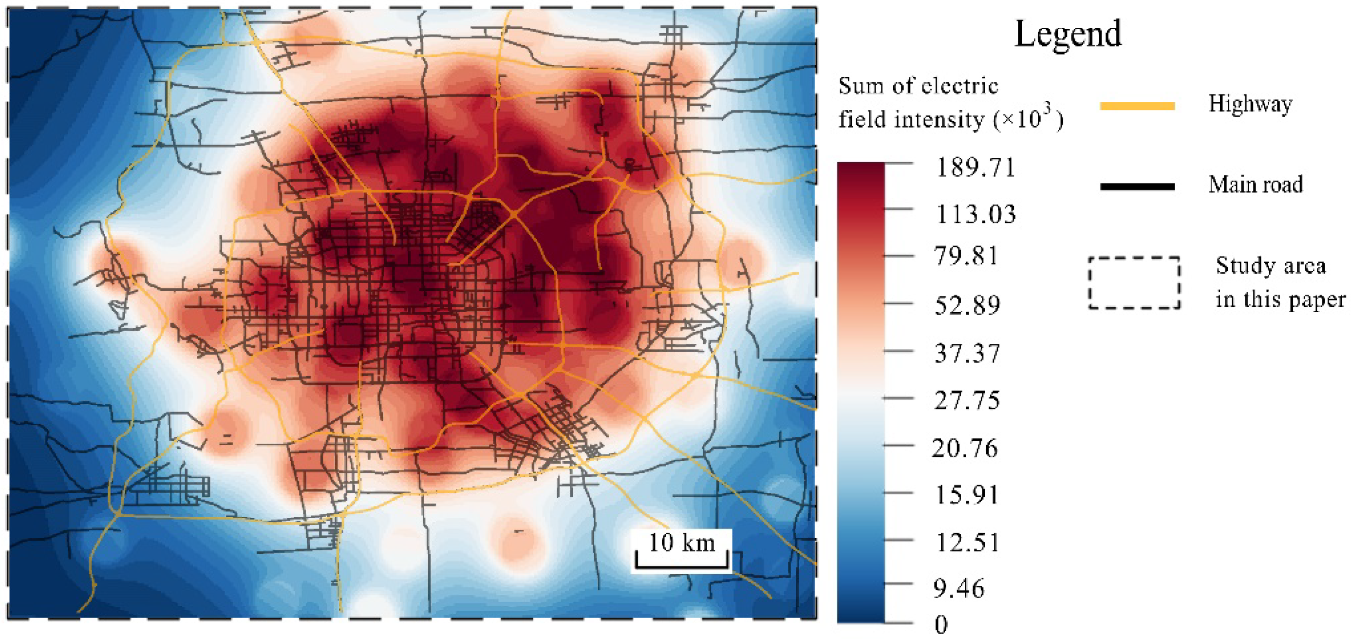
• The sum of the electric field intensities $\sum \left|\overrightarrow{E\left(r_{ji}\right)}\right|$ at a specific road point could reflect the importance of the road point to a certain extent. The road point has a greater probability of being a transportation hub or a transportation hotspot if the sum of the electric field intensities $\sum \left|\overrightarrow{E\left(r_{ji}\right)}\right|$ is bigger, since a bigger sum of the electric field intensities means that the road point is affected by more pick-up and drop-off hotspot clusters at a relatively close distance and bears more traffic-commuting pressure.
• The vector sum of the directions of the electric field $\overrightarrow{E\left(r_j\right)}$ at a road point can reflect the road-traffic commuting direction with the maximum probability at that point. The comprehensive performance of vehicles at a specific road point (denoted by $P_{\chi }$) tends to head in the same direction as the electric field at $P_{\chi }$, since that specific direction represents the direction of the commuting function undertaken by $P_{\chi }$ in the entire urban road-traffic commuting system.

3. Study Area and Data Resources

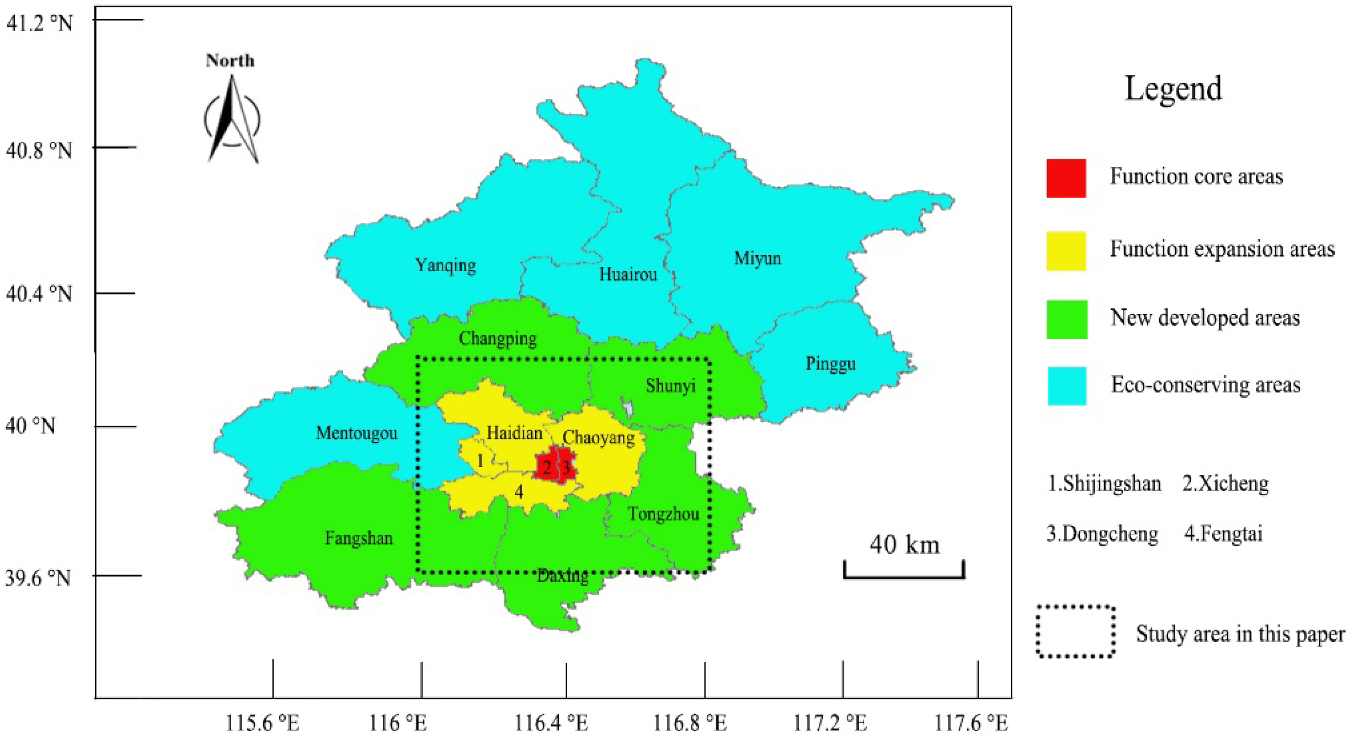
3.1. Study Area

Beijing occupies an area of 16,410 km² and hosts 21.73 million people, giving a population density of 1145 people/km² [38]. Beijing covers 16 administrative regions (Yanqing, Huairou, Miyun, Changping, Shunyi, Pinggu, Mentougou, Haidian, Chaoyang, Shijingshan, Xicheng, Dongcheng, Fengtai, Fangshan, Daxing, and Tongzhou). There is a total of four functional areas: core areas, expansion areas, new developed areas, and eco-conserving areas. As the traffic hotspots are mainly concentrated in the center of Beijing, we chose an area in this location as the study area. The study area is an approximate rectangle spanning 116 to 116.8° E and 39.6 to 40.2° N, and has an area of 4552.99 km². Figure 3 shows a map of Beijing which has been divided into districts according to administrative regions and functional areas [39].

Road traffic plays a critical role in connecting most people’s homes with their places of work or study. In Beijing, by June 2016, there were 21,885 km of public road, of which 982 km were highway. Figure 4 shows the road network of the study area. This figure shows only the highways, including the ring roads, and main roads, as they are the most important components of all the public roads, and typically enable the function of urban road-traffic commuting in a city. While some minor roads and paths may be chosen by pedestrians or cyclists, they do not play important roles in people’s long-distance commuting in a city, since these minor roads and paths mainly exist in communities, Hutongs (a type of narrow street or alley commonly associated with northern Chinese cities, especially Beijing), parks, etc.

3.2. Data Resources

There are two main modes of transport on roads in cities: private cars and public transport [40]. Private cars mainly include civilian vehicles, while public transport mainly includes buses and taxis. According to the Beijing census, there were a total of 5,474,400 civilian vehicles in Beijing in 2016 [38]. Of this number, 5,093,900 were civilian passenger service vehicles, 330,100 were civilian trucks, and 50,300 were other kinds of vehicles. All of these vehicles produce a huge volume of trajectory data at all times, however collecting all of this data is almost impossible due to the privacy restrictions in China. Taxis, another important kind of road-traffic vehicle, play an important role in transporting people. The trajectories of taxis are more flexible than those of buses. There were between 66,000 and 69,000 taxis in Beijing over the last several years, almost all of which are equipped with GPS recorders. According to previous studies, taxi trips represent a significant portion of people’s urban mobility [41]. For this study, we managed to obtain the GPS trajectory data from 66,646 taxis from the Beijing Municipal Commission of Transport. The data are from 30 September to 31 December 2012. The interval between two adjacent data records is one minute or several minutes, depending on the performance of the different GPS recorders. Each data record contains the following information: serial number, vehicle company, terminal ID, time label, WGS84 (World Geodetic System 1984) longitude, WGS84 latitude, mesh longitude, mesh latitude, vehicle speed, vehicle direction, vehicle state, event, and elevation. The most important pieces of information from the data records are terminal ID, time label, WGS84 longitude, WGS84 latitude, vehicle speed, and vehicle direction.

For our case study, we chose a total of 1,308,705 valid data records, i.e., those with no data deficiencies, recorded between 7:00 a.m. and 8:00 a.m. on working days.

4. Results

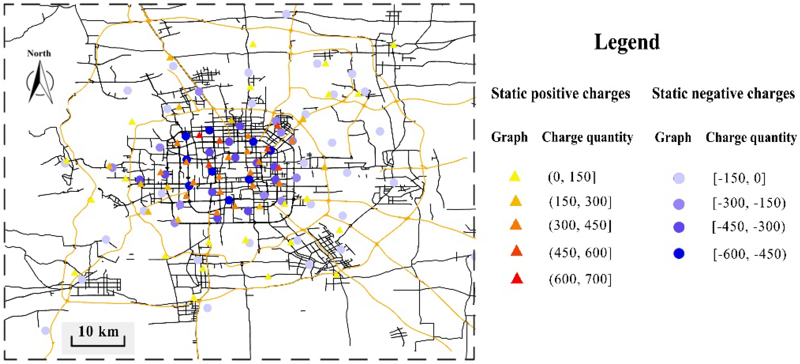
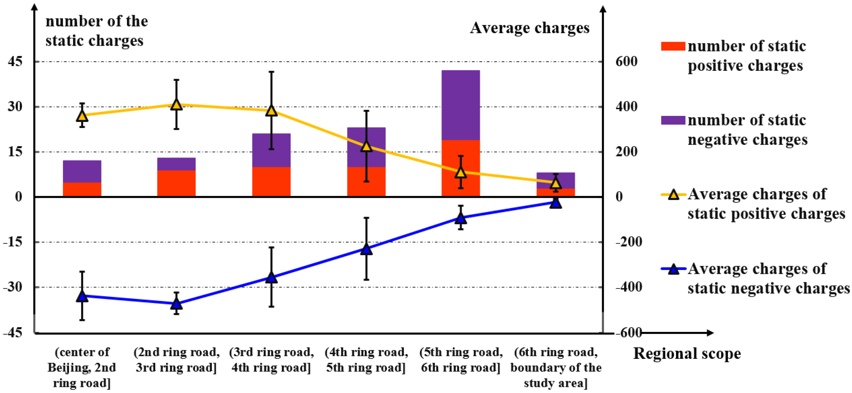
4.1. Features of the Urban Commuting Electric Field

The hotspot clusters can be obtained based on the O-D hotspot clustering model. The distribution of the hotspot cluster centers based on the O-D hotspot clustering model can be found in our previous study [35]. In the present study, the centers of the hotspot clusters are considered to be static charges. The pick-up hotspot clusters are considered to be static positive charges and the drop-off hotspot clusters are considered to be static negative charges. The distribution of the static charges in the case study is shown in Figure 5. The charge magnitude of these static charges is proportional to the number of pick-up or drop-off records in the study time interval.

There is a total of 56 static positive charges and 63 static negative charges in the study area, as shown in Figure 5. Traditionally, Chang’an Avenue, in front of Tiananmen Square, is considered to be the central point of Beijing. There are five ring roads in Beijing: the 2nd ring road to 6th ring roads. These ring roads divide the study area into six regions. The characteristics of static charges are shown in Figure 6. It was found that the number of static charges increases, with the exception of the area between the 6th ring road and the boundary of the study area, while the average charges fall when it is getting closer to the periphery of the city. This means that there are more static charges but fewer large static charges around the periphery of the city. It was found that most of the largest static charges are concentrated inside the 4th ring road. This means that the amount of commuter traffic within this region is the greatest for the same time interval. It was also found that the numbers of static positive charges and static negative charges are similar in each region, which means that job–housing balance has been a characteristic of the spatial distribution in the study area.

According to the assumptions made in Section 2.3, the sum of the electric field intensities $\sum \left|\overrightarrow{E\left(r_{ji}\right)}\right|$ at a specific road point reflects the importance of the road point to a certain extent. To prepare for later use in this study, the distribution of the sums of the electric field intensities $\sum \left|\overrightarrow{E\left(r_{ji}\right)}\right|$ in the study area was calculated. The result is shown in Figure 7. We found that it is easier to form a sub-circular area with a high sum of electric field intensities near the center of the study area. The sum of the electric field intensities is generally lower in the area close to the edge of the study area.

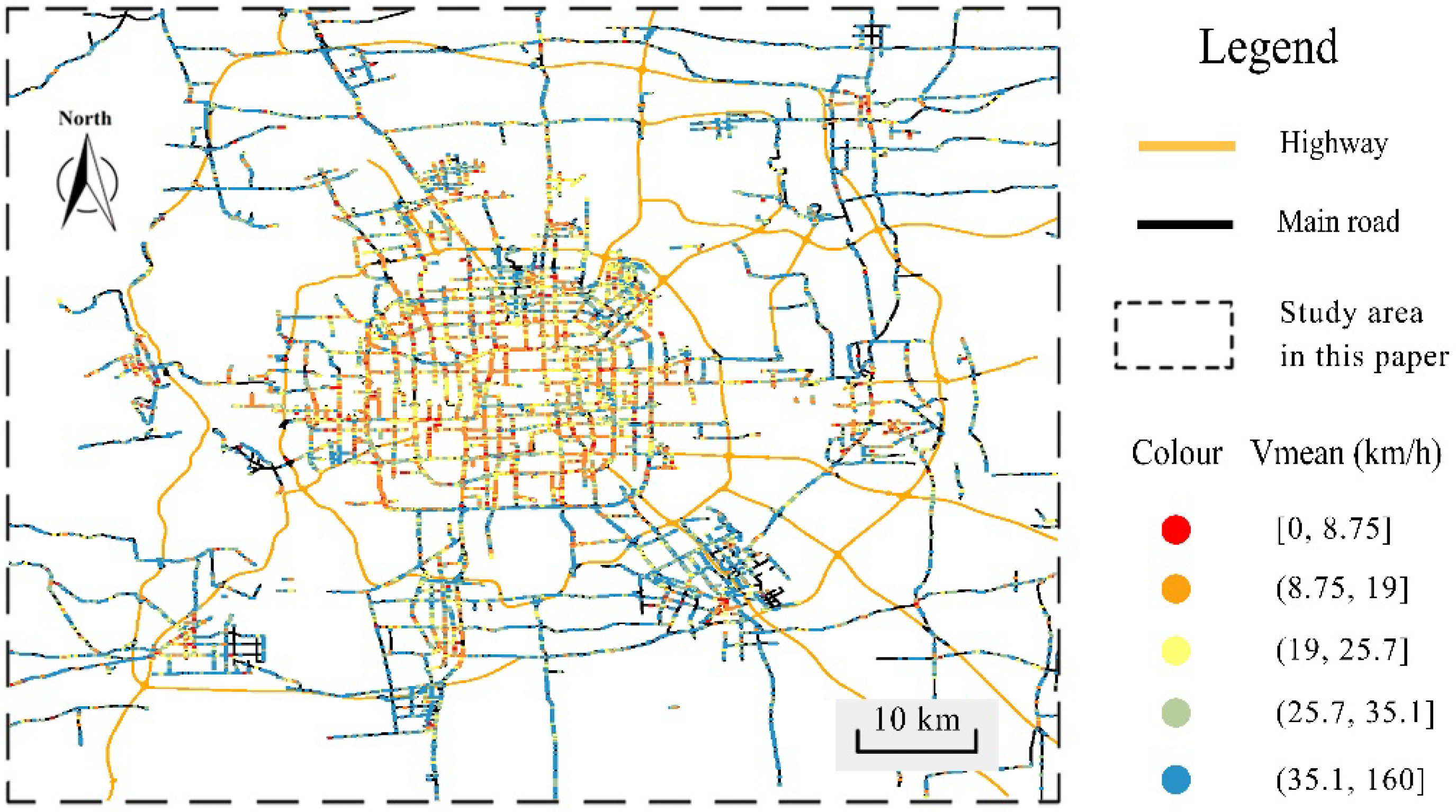
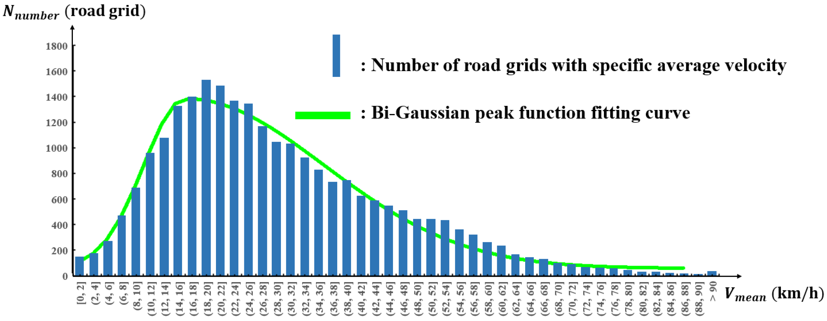
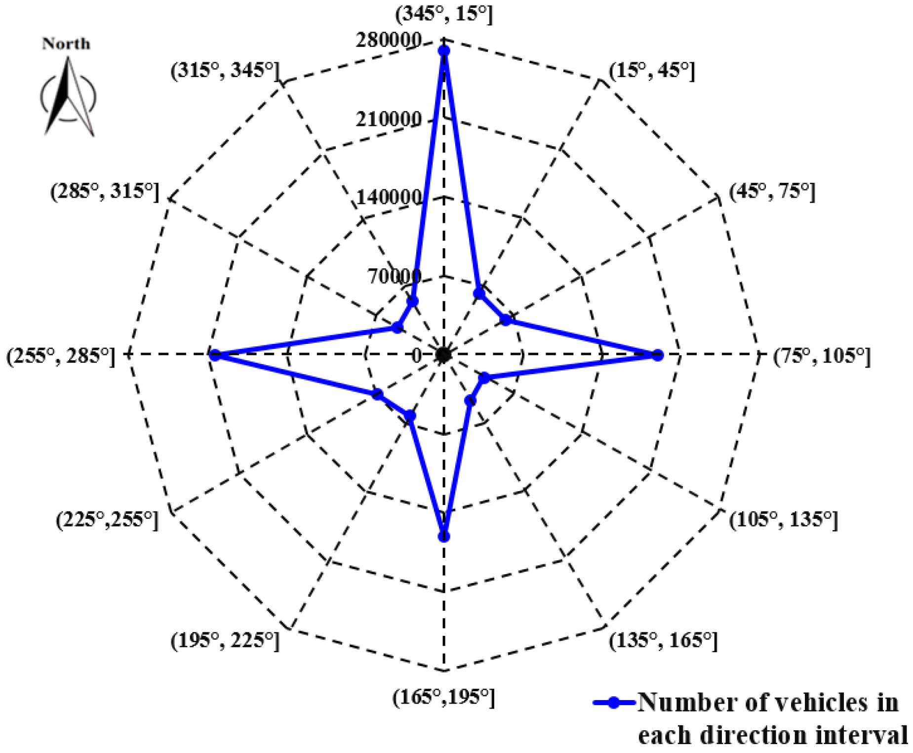
4.2. Features of Urban Road-Traffic Commuting

In this study, we analyzed the features of urban road-traffic commuting in two ways. The first was to individually analyze the statistical characteristics of 1,308,705 GPS data records of vehicle trajectories. The second was to cluster these GPS data records to the data-collection road points and then analyze the statistical characteristics of these road points. The first way can give an overall perspective of the data, however it requires immense computational resources and time. Considering that many GPS data records may have coverage near to the same road point, the second data processing method was a simple and effective way to process and present the data. A series of data-collection road points were set up every 100 meters on the highways and main roads, referred to as road grids. Then, the vehicles on the highways and main roads were clustered into these road grids according to the “nearest neighbor” principle. There was a total of 23,854 valid road grids in the study area.

The mean velocity of vehicles is the most important index for evaluating traffic flow conditions. The mean velocity of the vehicles in each road grid was calculated. The result is shown in Figure 8. In this figure, the intervals of the average velocity are divided into five groups: [0, 8.75], (8.75, 19], (19, 25.7], (25.7, 35.1], and (35.1, 160] (km/h). The widths of the intervals are not equal, in order to ensure that the number of clustered vehicles in each group is the same. Figure 8 also shows that the traffic condition is mainly in accordance with a two-ring structure. The mean velocity of vehicles outside Beijing’s 4th ring road largely falls in the range of (25.7, 160] km/h, with the color of the road grids being mainly green and blue. The mean velocity of vehicles in the core area of Beijing is generally less than 25.7 km/h, and the color of the road grids are mainly yellow, orange, or red.

The correlation between the number of road grids with specific average velocity, $N_{number},$ and the average velocity of vehicles, $V_{mean},$ in each road grid was quantitatively studied. The average velocity of vehicles was divided into 46 groups, with an interval length for the first 45 groups of 2 km/h. The interval of the last group is (90, 160] km/h. The histogram and fitted curve of the Bi-Gaussian peak function are shown in Figure 9. It can be seen that during the morning rush hour in Beijing, most road grids are in a “not fast” state, with a velocity in the interval of (8, 50] km/h. Moreover, there are a total of 8417 road grids with an average velocity in the interval of (14, 26] km/h, accounting for 34.75% of the total road grids—that is, a very high proportion of the road grids are in a “very slow” state.

The quantitative correlation between the number of road grids with specific average velocity $N_{number}$ and the average velocity of vehicles $V_{mean}$ can be very well represented by the following Bi-Gaussian peak function equation:

$$N_{number}\cong \{\begin{array}{c}54.00+1322.59·e^{-\frac{{\left(V_{mean}-16.51\right)}^2}{2} \times {6.11}^2}, V_{mean}<16.51\hfill \\ 54.00+1322.59·e^{-\frac{{\left(V_{mean}-16.51\right)}^2}{2} \times {20.20}^2}, V_{mean}\ge 16.51\hfill \end{array}, R^2=0.981$$

(16)

The direction in which vehicles are heading is another important index for monitoring traffic flow conditions. We calculated the direction of each vehicle from 1,308,705 individual GPS data records. The result is shown in Figure 10. The numbers of vehicles heading in the direction intervals (345°, 15°], (75°, 105°], (165°, 195°], and (255°, 285°] are 269,320, 189,222, 161,221, and 203,597, respectively, accounting for 21.22%, 14.91%, 12.71%, and 16.04% of the total, respectively. These figures show that most vehicles in the study area moved in a north-south and east-west direction. This is in accordance with the road layout in the study area, since most highways and main roads in Beijing are arranged in the north-south and east-west directions.

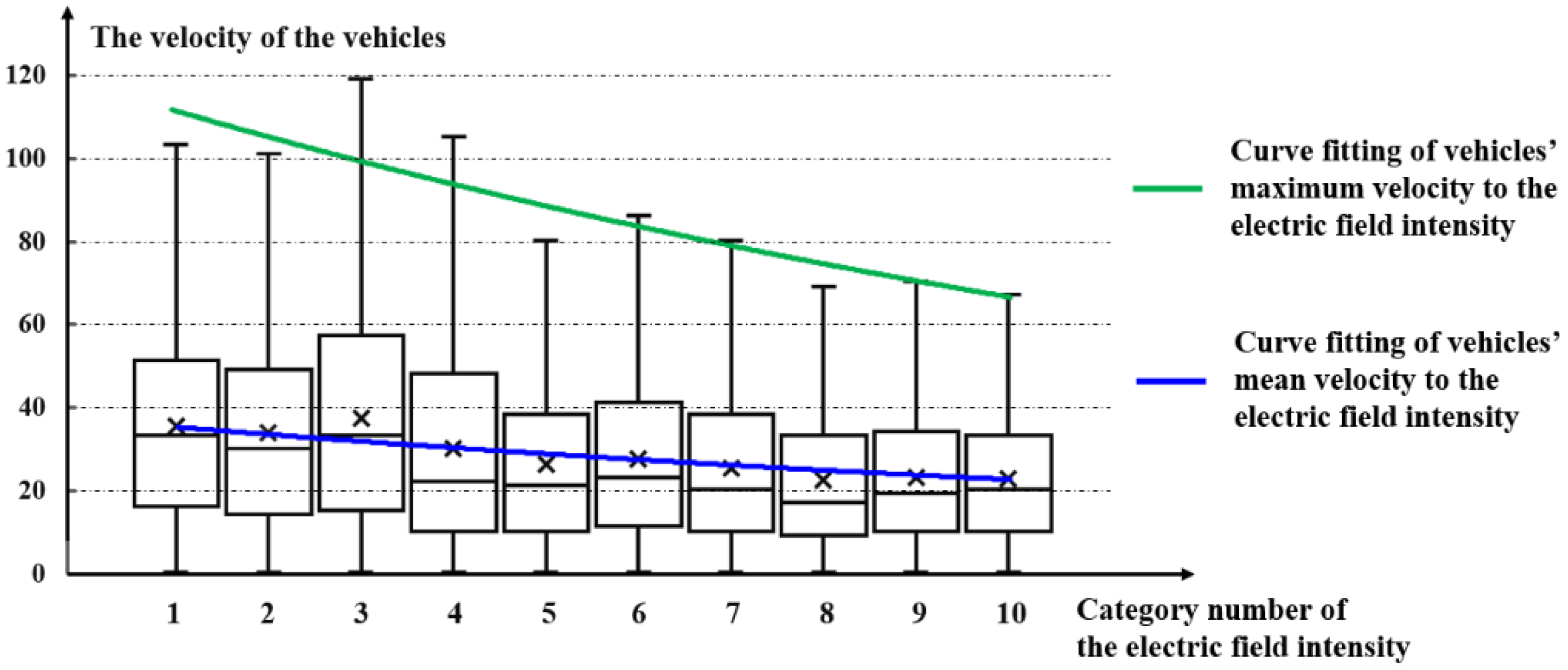
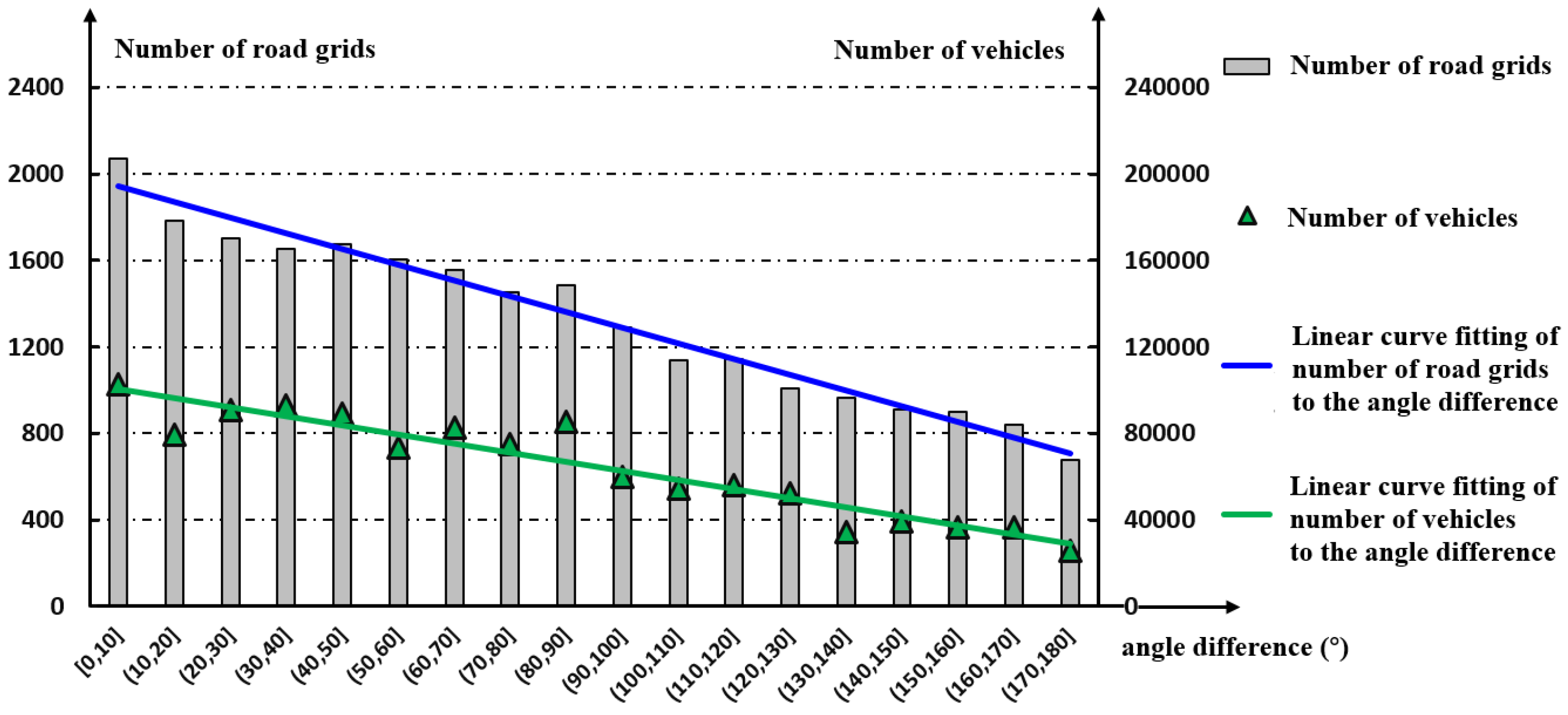
4.3. Correlation between the Urban Commuting Electric Field and Urban Road-Traffic Commuting

To verify the two assumptions made in Section 2.3 and to study any correlation between the urban commuting electric field and the urban road-traffic commuting, the GPS data records of vehicle trajectories were clustered to the road grids (as shown in Figure 11) and the intensities and directions of the urban commuting electric field at these road grids were calculated. From the geographic data of Beijing, we obtained 39,500 road grids from highways and main roads. After data processing, there was a total of 23,854 valid road grids used for this study.

According to the first assumption made in Section 2.3, the sum of the electric field intensities $\sum \left|\overrightarrow{E\left(r_{ji}\right)}\right|$ at a specific road grid usually reflects the importance of the road grid to a certain extent. Some previous studies have proved that there is a physical relationship between the density of traffic and the average speed of vehicles [42]. Therefore, road grids with higher importance will be more likely to have a slow traffic condition, since the bottleneck of the road-traffic network with a high density of traffic usually exists where the centrality of the network is higher. It also follows that the maximum velocity and the mean velocity of vehicles at a road grid with higher importance will be slower. The detailed correlation between the maximum velocity and mean velocity of the vehicles and the sum of the electric field intensities $\sum \left|\overrightarrow{E\left(r_{ji}\right)}\right|$ is shown in Figure 12. According to the results shown in Figure 7, the sums of the electric field intensities $\sum \left|\overrightarrow{E\left(r_{ji}\right)}\right|$ are divided into 10 groups to ensure that the data recorders in each group are the same. The category numbers and the corresponding intervals of $\sum \left|\overrightarrow{E\left(r_{ji}\right)}\right| \left(\times {10}^3\right)$ are as follows: ①$(0, 9.46]$, ②$(9.46, 12.51]$, ③$(12.51, 15.91]$, ④$(15.91, 20.76]$, ⑤$(20.76, 27.75]$, ⑥$(27.75, 37.37]$, ⑦$(37.37, 52.89]$, ⑧$(52.89, 79.81]$, ⑨$(79.81, 113.03]$, ⑩$(113.03, 189.71)$. We found that as the sum of the electric field intensities increases, both the maximum velocity and the mean velocity of vehicles have a significant tendency to decrease. This means that the areas with high electric field intensity calculated by the urban commuting electrostatics model are more likely to be slow traffic areas.

.

According to the second assumption made in Section 2.3, the overall direction that vehicles take tends to be the same as the direction of the electric field. To verify this assumption, we calculated the vector sum of the velocities of vehicles in each valid road grid. As is well known, the vector sum of the velocities of two vehicles traveling at the same speed but in opposite directions is zero. Thus, the vector sum of the velocities of vehicles in the road grids can offset the velocities of some vehicles traveling in the opposite direction, and can reflect the comprehensive direction of the velocities of the vehicles in those grids. The vector sum of the directions of the electric field $\overrightarrow{E\left(r_j\right)}$ at a road point is easy to calculate based on the urban commuting electrostatics model. The angle between the vector sum of the velocities of vehicles at the road grids and the vector sum of the directions of the electric field $\overrightarrow{E\left(r_j\right)}$ at that same road point is denoted by $\left|\delta \theta \right|$. This difference $\left|\delta \theta \right|$ is divided into 18 groups. These intervals are identified by ${⟦|\delta \theta |⟧}_i, i=1,2,\dots ,18$. We studied the detailed correlation between the number of valid road grids and the number of vehicles clustered in the road grids to ${⟦|\delta \theta |⟧}_i \left(i=1,2,\dots ,18\right)$. The results are shown in Figure 13. In Figure 13, ${⟦|\delta \theta |⟧}_1=[0,10],{⟦|\delta \theta |⟧}_i=\left(10\times \left(i-1\right),10\times i\right], i=2,3,\dots ,18$.

The quantitative relationship between the number of road grids and the angle difference interval ${⟦|\delta \theta |⟧}_i$ can be expressed by the following equation, where ${⟦|\delta \theta |⟧}_{i\varpi }$ is the intermediate value of the angle difference interval ${⟦|\delta \theta |⟧}_i$:

$$N_{road grid}\cong -7.24\times {⟦|\delta \theta |⟧}_{i\varpi } +1.98\times {10}^3, R^2=0.971$$

(17)

The quantitative relationship between the number of vehicles and the angle difference interval ${⟦|\delta \theta |⟧}_i$ can be expressed by the following equation:

$$N_{vehicles}\cong -424.01\times {⟦|\delta \theta |⟧}_{i\varpi }+1.03\times {10}^5, R^2=0.971$$

(18)

We found that as the upper limits and the lower limits of the angle difference intervals increase, the number of eligible road grids and the number of eligible vehicles have a significant tendency to decrease. This means that the comprehensive trajectory of vehicles in most road grids tends to be along the direction of the electric field calculated from the urban commuting electrostatics model. With increasing angle difference $\left|\delta \theta \right|$, the number of road grids and that of vehicles decrease.

5. Discussion and Conclusions

The initial aims were how to analyze the characteristics of commuting generations and the characteristics of commuting dynamics using GPS trajectories, and then to clarify the relationship between them. We tried to solve these problems by establishing a set of simple, universal, and effective methods. In this paper, we made an analogy between urban traffic and electrostatics. This set of methods used includes several steps. First, an O-D hotspot clustering model was used to discover the O-D hotspots. Then, the core idea of the methods was introduced, namely that the spatial migration of people by vehicles was considered to be the outcome of a repulsion force from the pick-up origin and an attraction force from the drop-off destination. A two-dimensional urban commuting electric field was built based on this idea. Afterwards, we researched the features of the urban commuting generations, the features of urban road-traffic commuting, and the correlation between them.

As a case study, we chose to study the core area of Beijing, which covers an area of 4552.99 km², based on 1,308,705 valid GPS data records of vehicle trajectories from consecutive work days between the hours of 7:00 a.m. and 8:00 a.m. The models allowed us to obtain some significant findings, including the spatial distribution and characteristics of O-D hotspots, the ring structure of cities, the velocity distribution of vehicles, and the direction distribution of vehicles. Among all the results, the most important conclusion is that as the electric field intensity calculated by the urban commuting electrostatics model increases, both the maximum velocity of vehicles and the mean velocity of vehicles have a significant tendency to decrease. This means that areas with high electric field intensity calculated by the urban commuting electrostatics model are more likely to have slow traffic. We use $\left|\delta \theta \right|$ to denote the angle between the vector sum of the velocities of vehicles at the road grids and the vector sum of the directions of the electric field at that same road point. Another important discovery is that as $\left|\delta \theta \right|$ increases, the number of eligible road grids and the number of eligible vehicles have a significant tendency to decrease. This means that the comprehensive performance of vehicles at most road grids tends to head along the direction of the electric field calculated by the urban commuting electrostatics model.

The results reflect that the models have the advantage of being able to analyze the urban road-traffic commuting dynamics in a unique way. The results above verify that the set of methods, including the proposed model, is valid to be used as a tool for analyzing the urban commuting generations and the features of urban road-traffic commuting, based on which the correlation between them can be clarified. The models proposed in this paper and the corresponding results provide a new perspective for understanding the mechanisms of urban road-traffic commuting. The model can also be used for urban zone and traffic network planning.

Future research could be conducted based on expanded datasets, following which the relationship between urban road-traffic commuting dynamics modeled using taxi trajectories and those modeled using more datasets could be explored in depth.

References

- Tabuchi, T. Urban agglomeration and dispersion: A synthesis of alonso and krugman. J. Urban Econ. 1998, 44, 333–351. [Google Scholar] [CrossRef]
- David, M.; Nicholas, S.W.; Julia, F.; Brad, W. Use our infographics to explore the rise of the urban planet. Science. 2016. Available online: http://www.sciencemag.org/news/2016/05/use-our-infographics-explore-rise-urban-planet (accessed on 14 November 2018). [CrossRef]
- Agryzkov, T.; Oliver, J.L.; Tortosa, L.; Vicent, J.F. Analyzing the commercial activities of a street network by ranking their nodes: A case study in Murcia, Spain. Int. J. Geogr. Inf. Sci. 2014, 28, 479–495. [Google Scholar] [CrossRef]
- Yao, Z.Y.; Kim, C. The Changes of Urban Structure and Commuting: An Application to Metropolitan Statistical Areas in the United States. Int. Reg. Sci. Rev. 2019, 42, 3–30. [Google Scholar] [CrossRef]
- Duarte, C.M.; Fernández, M.T. The Influence of Urban Structure on Commuting: An Analysis for the Main Metropolitan Systems in Spain. In Proceedings of the Urban Transitions Conference, Shanghai, China, 5–9 September 2016. [Google Scholar] [CrossRef]
- Andersson, M.; Lavesson, N.; Niedomysl, T. Rural to urban long-distance commuting in Sweden: Trends, characteristics and pathways. J. Rural Stud. 2018, 59, 67–77. [Google Scholar] [CrossRef]
- Ma, X.L.; Zhang, J.Y.; Ding, C.; Wang, Y.P. A geographically and temporally weighted regression model to explore the spatiotemporal influence of built environment on transit ridership. Comput. Environ. Urban Syst. 2018, 70, 113–124. [Google Scholar] [CrossRef]
- Salas-Olmedo, M.H.; Nogués, S. Analysis of commuting needs using graph theory and census data: A comparison between two medium-sized cities in the UK. Appl. Geogr. 2012, 35, 132–141. [Google Scholar] [CrossRef]
- Hiribarren, G.; Herrera, J.C. Real time traffic states estimation on arterials based on trajectory data. Transp. Res. B 2014, 69, 19–30. [Google Scholar] [CrossRef]
- Cole-Hunter, T.; Donaire-Gonzalez, D.; Curto, A.; Ambros, A.; Valentin, A.; Garcia-Aymerich, J.; Martínez, D.; Braun, L.M.; Mendez, M.; Jerrett, M.; et al. Objective correlates and determinants of bicycle commuting propensity in an urban environment. Transp. Res. D 2015, 40, 132–143. [Google Scholar] [CrossRef]
- Nasri, A.; Zhang, L. Multi-level urban form and commuting mode share in rail station areas across the United States; a seemingly unrelated regression approach. Transp. Policy 2018, 5. [Google Scholar] [CrossRef]
- Ma, X.L.; Liu, C.C.; Wen, H.M.; Wang, Y.P.; Wu, Y.J. Understanding commuting patterns using transit smart card data. J. Transp. Geogr. 2017, 58, 135–145. [Google Scholar] [CrossRef]
- Chae, J.; Thom, D.; Jang, Y.; Kim, S.Y.; Ertl, T.; Ebert, D.S. Public behavior response analysis in disaster events utilizing visual analytics of microblog data Computers & Graphics. Comput. Graph. 2014, 38, 51–60. [Google Scholar] [CrossRef]
- Sun, C.S.; Pei, X.; Hao, J.H.; Wang, Y.W.; Zhang, Z. Role of road network features in the evaluation of incident impacts on urban traffic mobility. Transp. Res. B 2018, 117, 101–116. [Google Scholar] [CrossRef]
- Agryzkov, T.; Oliver, J.L.; Tortosa, L.; Vicent, J.F. An algorithm for ranking the nodes of an urban network based on the concept of PageRank vector. Appl. Math. Comput. 2012, 219, 2186–2193. [Google Scholar] [CrossRef]
- Agryzkov, T.; Marti, P.; Tortosa, L.; Vicent, J.F. Measuring urban activities using Foursquare data and network analysis: A case study of Murcia (Spain). Int. J. Geogr. Inf. Sci. 2017, 31, 100–121. [Google Scholar] [CrossRef]
- Zhang, X.Y.; Li, W.W.; Zhang, F.; Liu, R.Y.; Du, Z.H. Identifying Urban Functional Zones Using Public Bicycle Rental Records and Point-of-Interest Data. ISPRS Int. J. Geo-Inf. 2018, 7, 459. [Google Scholar] [CrossRef]
- Wan, L.; Gao, S.; Wu, C.; Jin, Y.; Mao, M.R.; Yang, L. Big data and urban system model—Substitutes or complements? A case study of modelling commuting patterns in Beijing. Comput. Environ. Urban Syst. 2018, 68, 64–77. [Google Scholar] [CrossRef]
- Misra, A. Using vehicular data to understand urban mobility & events. In Proceedings of the 2017 IEEE 42nd Conference on Local Computer Networks: Workshops, Singapore, 14–17 October 2017. [Google Scholar] [CrossRef]
- Sun, J.P.; Wen, H.M.; Gao, Y.; Hu, Z.W. Metropolitan Congestion Performance Measures Based on Mass Floating Car Data. In Proceedings of the International Joint Conference on Computational Sciences and Optimization, Sanya, China, 24–26 April 2009. [Google Scholar] [CrossRef]
- Fu, X.; Sun, M.P.; Sun, H. Taxi Commute Recognition and Temporal-spatial Characteristics Analysis Based on GPS Data. China J. Highw. Transp. 2017, 30, 134–143. [Google Scholar] [CrossRef]
- Mao, F.; Ji, M.H.; Liu, T. Mining spatiotemporal patterns of urban dwellers from taxi trajectory data. Front. Earth Sci. 2016, 10, 205–221. [Google Scholar] [CrossRef]
- Casey, H.J. Applications to traffic engineering of the law of retail gravitation. Traff. Q. 1955, IX, 23–25. [Google Scholar]
- Krings, G.; Calabrese, F.; Ratti, C.; Blondel, V.D. Scaling behaviors in the communication network between cities. In Proceedings of the 12th IEEE International Conference on Computational Science and Engineering, CSE, Vancouver, BC, Canada, 29–31 August 2009. [Google Scholar] [CrossRef]
- Ortúzar, J.D.; Willumsen, L.G. Trips distribution modelling. In Modelling Transport, 4th ed.; John Wiley & Sons, Ltd.: Hoboken, NJ, USA, 2011; p. 182. [Google Scholar]
- Yang, Y.D.; Fan, Y.Y.; Wets, R.J.B. Stochastic travel demand estimation: Improving network identifiability using multi-day observation sets. Transp. Res. B 2018, 107, 192–211. [Google Scholar] [CrossRef]
- Gao, J.R.; Yu, B.; Pan, D.Z. Accurate lithography hotspot detection based on PCA-SVM classifier with hierarchical data clustering. In Proceedings of the SPIE-The International Society for Optical Engineering, Design-Process-Technology Co-Optimization for Manufacturability VIII, San Jose, CA, USA, 26–27 February 2014. [Google Scholar] [CrossRef]
- Wang, L.; Hu, K.Y.; Ku, T.; Wu, J.W. Urban mobility dynamics based on flexible discrete region partition. Int. J. Distrib. Sens. Netw. 2014, 2014, 782649. [Google Scholar] [CrossRef]
- Zhang, P.D.; Deng, M.; Shi, Y.; Zhao, L. Detecting hotspots of urban residents’ behaviours based on spatio-temporal clustering techniques. GeoJournal 2017, 82, 923–935. [Google Scholar] [CrossRef]
- Schoier, G.; Borruso, G. Spatial data mining for highlighting hotspots in personal navigation routes. Int. J. Data Warehous. 2012, 8, 45–61. [Google Scholar] [CrossRef][Green Version]
- Qin, K.; Zhou, Q.; Wu, T.; Xu, Y.Q. Hotspots detection from trajectory data based on spatiotemporal data field clustering. International Archives of the Photogrammetry. Remote Sens. Spat. Inf. Sci.-ISPRS Arch. 2017, 42, 1319–1325. [Google Scholar] [CrossRef]
- Hussain, S.F.; Haris, M. A k-means based co-clustering (kCC) algorithm for sparse, high dimensional data. Expert Syst. Appl. 2019, 118, 20–34. [Google Scholar] [CrossRef]
- Li, M.C.; Han, S.; Shi, J. An enhanced ISODATA algorithm for recognizing multiple electric appliances from the aggregated power consumption dataset. Energy Build. 2017, 140, 305–316. [Google Scholar] [CrossRef]
- Liu, Q.J.; Zhao, Z.M.; Li, Y.X.; Li, Y.Y. Feature selection based on sensitivity analysis of fuzzy ISODATA. Neurocomputing 2012, 85, 29–37. [Google Scholar] [CrossRef]
- Ni, X.Y.; Huang, H.; Zhou, S.W.; Su, B.N.; Meng, Y.Y.; Huang, Z.L. Spatial data mining and O-D hotspots discovery in cities based on an O-D hotspots clustering model using vehicles’ GPS data—A case study in the morning rush hours in Beijing, China. In Proceedings of the 4th ACM SIGSPATIAL International Workshop on Safety and Resilience 2018, Seattle, WA, USA, 6–9 November 2018. [Google Scholar] [CrossRef]
- Clustering Algorithm-ISODATA Algorithm. Available online: https://www.cnblogs.com/huadongw/articles/4101306.html (accessed on 20 January 2019).
- Zhang, N.; Li, Y.G. A human behavior integrated hierarchical model of airborne disease transmission in a large city. Build. Environ. 2017, 127, 211–220. [Google Scholar] [CrossRef]
- Annual Data of the Province in China. Available online: http://data.stats.gov.cn/easyquery.htm?cn=E0103 (accessed on 1 August 2018).
- Ni, X.Y.; Huang, H.; Du, W.P. Relevance analysis and short-term prediction of PM2.5 concentrations in Beijing based on multi-source data. Atmos. Environ. 2017, 150, 146–161. [Google Scholar] [CrossRef]
- Li, Q.; Liao, F.X.; Timmermans, H.J.P.; Huang, H.; Zhou, J. Incorporating free-floating car-sharing into an activity-based dynamic user equilibrium model: A demand-side model. Transp. Res. B 2018, 107, 102–123. [Google Scholar] [CrossRef]
- Yuan, N.J.; Zheng, Y.; Xie, X.; Wang, Y.Z.; Zheng, K.; Xiong, H. Discovering urban functional zones using latent activity trajectories. IEEE Trans. Knowl. Data Eng. 2015, 27, 712–725. [Google Scholar] [CrossRef]
- Hörcher, D.; Graham, D.J.; Anderson, R.J. Crowding cost estimation with large scale smart card and vehicle location data. Transp. Res. B 2017, 95, 105–125. [Google Scholar] [CrossRef]