Quality Control of “As Built” BIM Datasets Using the ISO 19157 Framework and a Multiple Hypothesis Testing Method Based on Proportions

Abstract

Building information model (BIM) data are digital and geometric-based data that are enriched thematically, semantically, and relationally, and are conceptually very similar to geographic information. In this paper, we propose both the use of the international standard ISO 19157 for the adequate formulation of the quality control for BIM datasets and a statistical approach based on a binomial/multinomial or hypergeometric (univariate/multivariate) model and a multiple hypothesis testing method. The use of ISO 19157 means that the definition of data quality units conforms to data quality elements and well-defined scopes, but also that the evaluation method and conformity levels use standardized measures. To achieve an accept/reject decision for quality control, a statistical model is needed. Statistical methods allow one to limit the risks of the parties (producer and user risks). In this way, several statistical models, based on proportions, are proposed and we illustrate how to apply several quality controls together (multiple hypothesis testing). All use cases, where the comparison of a BIM dataset versus reality is needed, are appropriate situations in which to apply this method in order to supply a general digital model of reality. An example of its application is developed to control an “as-built” BIM dataset where sampling is needed. This example refers to a simple residential building with four floors, composed of a basement garage, two commercial premises, four apartments, and an attic. The example is composed of six quality controls that are considered simultaneously. The controls are defined in a rigorous manner using ISO 19157, by means of categories, scopes, data quality elements, quality measures, compliance levels, etc. The example results in the rejection of the BIM dataset. The presented method is, therefore, adequate for controlling BIM datasets.

1. Introduction

From an informational point of view, a Building information model (BIM) refers to digital model-based geometric information, which is enriched thematically, semantically, and relationally; managed by the right software tools, a BIM allows for the smarter management of buildings and facilities. The cornerstone of BIMs is to understand the relationships between materials, objects, assemblies, and projects [1]. All these elements are managed by a BIM tool as objects, in the same sense as object-oriented programming [2]. This means that materials, objects, assemblies, and projects have properties, methods, events, and relationships. However, objects are not only the way information is handled by database programs; objects are also a way to understand and organize the world. In a BIM, objects carry information about identity, appearance, behavior, use, age, location, components, restrictions, or rules, etc. All this information is managed by the BIM tool as a database. Even though Weigant [1] stated that BIM tools are “little more than a database management system” almost 10 years ago, much has happened since then, enabling designers to work smarter today through improved interoperability, automation, visual programming, simulation, etc. From this point of view, BIM tools are directly linked to advanced Geographic Information Systems (GIS) and BIM data to spatial data (geographic information). In this way, Sun et al. [3] showed that close links exist between spatial data and BIM data, and Song et al. [4] indicated the need for, and potential profits from, the integration of BIM and GIS.

In some countries, there is a legal requirement for the use of BIMs for certain types of investments or public works (e.g., the United Kingdom, Netherlands, Denmark, Finland, and Norway), and for the European Union, it is regulated by Directive 2014/24, EU 2014, which mandates the use of BIM in construction projects financed by EU public funds. Under these regulations, the interchange of BIM datasets between agents (contractors, material manufacturers, producers, architects, end users, asset managers, etc.) will be more relevant and problematic [5]. In this, framework the data quality of BIM datasets is relevant, and the BIM Community (www.bimcommunity.com/) has developed a publication series that includes a guide centered on the quality assurance of BIM projects [6]. This document proposes and develops several quality controls, mainly devoted to checking logical consistency issues (e.g., topological rules, the domain consistency of attributes, format consistency, etc.), and the use of software is proposed for examining clashes between building elements.

Puyan et al. [7] highlight the interest and importance of the quality of BIM data for facility management purposes and present six examples of errors in BIM data that are very similar to those that occur in spatial data. In any case, the most relevant contribution is the proposal of a detailed framework for creating and performing BIM information quality assurance tests for asset and space management purposes. Donato et al. [8] proposed a quality assurance procedure for the architectural design process based on customized checklists and queries. Park et al. [9] executed rule-based and visualization-based checking procedures as a method for quality control centered on resolving building safety issues. Automatic routines for the quality control of BIM have been proposed by Cheng [10] and many other authors. Additionally, several software tools for this purpose have been developed, such as iTWO by RIB [11] and Solibri by Solibri (www.solibri.com); BIM Tree Manager by Agacad (www.aga-cad.com); and Verity by ClearEdge (www.clearedge3d.com). All these controls are based on aspects of logical consistency that, in most cases, can be automated. Therefore, statistical methods based on sampling and statistical tests are not required. However, this is a clear limitation because the aforementioned automated controls are not able to verify the delivery of a BIM database against reality (i.e., the situation “as is”). This BIM database can result from the BIM design process or from a survey of attributes and geometries from existing construction.

Neither of the previously mentioned documents or tools develop or propose a method for statistical quality control, nor is there any mention of quality control standards from the industrial field (e.g., the ISO 2851 or ISO 3851 series). Within this statistical perspective, Cheok et al. [12,13,14] proposed a statistical model adopted by the National Institute of Standards and Technology (NIST) of the United States, which is based on a binomial model. This proposal was created to manage the 3D captures of more than 1600 buildings and the production of BIM models by the General Services Administration [12]. This study only considers measures of the dimensions of elements that are converted to binomial variables by means of the simultaneous application of two criteria. Here, it is interesting to note that the binomial model, which is characteristic of qualitative variables (e.g., non-numerical values as the presence or absence of elements), is applied to quantitative variables (e.g., the numerical values of measurements). This offers greater simplicity in statistical processes. When comparing a dataset against the real world, the control process cannot be automated, and a representative sample from reality is required. Thus, the NIST control method requires an analysis of reality to determine dimensional errors. To execute the control, a random sampling of size $n$ is carried out after the total of the observed items is checked and the total measurements outside tolerance are determined against a value given by tables. If the total observed measurements outside tolerance exceed the value indicated in the tables for a given population and sample size, the specifications are not met. Nevertheless, this method uses a confidence interval perspective and does not use a hypothesis test approach.

The situation described above indicates the existence of several aspects that require research attention. For example, all aspects whose quality must be controlled in BIM datasets must be formalized. Additionally, an appropriate method must be available so that the acceptance/rejection of BIM datasets can be carried out on a statistical basis when sampling is needed (e.g., as a built perspective). In this work, proposals are made in these two categories. Thus, our objective is to propose how to adequately formulate quality control for BIM datasets and how to approach statistical control. In this work, we focus on the case of “as built” models. In this case, quality control based on hypothesis testing and statistical sampling is required. This situation is more complex than performing automated controls on 100% of the elements, so a general statistical model is needed. Considering a model of a building, this work is of interest to both the producers of BIM datasets and the recipients (users of the BIM model), as it offers a framework for the acceptance/rejection of BIM data products.

This paper is organized as follows, after this introduction, the adopted ISO 19157 [15] model for dealing with data quality elements is presented, in which a new data quality element is defined. After this, the fundamentals of quality control (hypothesis testing), based on counting, are presented. Next, we present several explanations to facilitate the applicability of the statistical methods to actual cases where quantitative and qualitative elements are jointly presented, but also where the seriousness of defects and joint controls are a common occurrence. An actual example is then shown, taking into account the most important issues (e.g., the definition of categories of interest, scopes, etc.), where six controls are performed jointly, and three different base statistical models are considered. Finally, the conclusions are presented. Additionally, two appendices are included (A and B). Appendix A shows the statistical models for working with a single category (binomial and hypergeometric models) or with multiple categories (multinomial and multivariate hypergeometric models), depending on whether the population to be controlled can be considered infinite (binomial and multinomial cases) or finite (hypergeometric cases). Appendix B shows a calculation example that is valid for a multivariate hypergeometric case. Finally, a list of acronyms has been added.

2. BIM Data Quality Elements

As indicated by Yang et al. [16], data quality is somewhat difficult to define precisely, as it means different things to different user communities. For this reason, in the field of data quality, there are several models/frameworks used to address different realities. For example, there are several international ISO standards offering different perspectives on data quality. The model established by ISO 8000 standards [17,18] allows the industrial data perspective to be approached, an appropriate perspective for assembly (e.g., in the military, aerospace, or naval industries). ISO/IEC 25012 [19] defines a general data quality model for data within computer systems, and ISO/TR 21707 [20] handles the quality of data being exchanged between the agents of the intelligent transportation system domain. The International Standard ISO 19157 [15] establishes the principles for describing the quality of spatial data.

BIM data are similar to spatial data because they must be integrated into a geographical framework (the actual location of the building), integrated into the environment (the surrounding geographical-topographic reality), and must collect the presence, dimensions, positions, and exact attributes of the elements of interest. This resemblance is both conceptual (data models) and factual (e.g., the capture and processing procedures), and also refers to exploitation (thematic, topological, temporal consultations, modeling, etc.). This proximity facilitates an advantageous approximation since, in the field of geographic information, there is greater emphasis placed on data quality. For instance, Sun et al. [3] showed the close links between spatial data and BIM data and presented a review of the standards and methods currently used for ensuring quality in spatial data and BIM in Sweden (mainly), as well as internationally. For this reason, we adopt this international standard as the basis for our proposal.

The International Standard ISO 19157 establishes the principles for describing the quality of spatial data. This is achieved by defining the data quality elements, data quality measures, and a general procedure for assessing and reporting data quality.

As a way of handling diverse perspectives of data quality, ISO 19157 proposes so-called data quality elements (DQEs). A DQE relates to the specific aspects of data quality that can be measured and evaluated through different measures and methods. DQEs are related to intrinsic data quality cues and can be organized into logically grouped categories (e.g., all DQEs related to logical consistency conform to a category). In accordance with the stated objective of focusing on the control of “as built” cases (that is, the BIM database versus reality), the following proposal is made for categories and DQEs that must be verified against reality:

• Completeness of data: This category (DQ_Completeness) refers to the presence and absence of objects, their attributes, and relationships. Lack of completeness is important when working with data that reflect reality. For example, a door or window cannot be missing in BIM data. In this case, two DQEs can be considered:

  ○

  Commission: The presence of excess data within the BIM Data. This means that some objects appearing in the BIM data do not exist in the real world.

  ○

  Omission: The absence of certain data within the BIM data. This means that some objects not included in the BIM model exist in the real world.

• Metric accuracy: This category name does not appear in ISO 19157, where it appears instead as positional accuracy (DQ_PositionalAccuracy). Our current proposal is broad, however, and allows the scheme developed in ISO 19157 to be generalized. In this case, the following DQEs are proposed:

  ○

  Absolute positional accuracy: The precise location in the geographical space of buildings and civil works is fundamental. We believe that BIMs should be understood as fully integrated with geographic information and geoservices (e.g., spatial data infrastructures, virtual balloons, etc.). This means that absolute positional accuracy is a critical aspect, and a coordinate reference system and projection is required, if necessary. For example, absolute positional accuracy will be a requirement to properly integrate a BIM model with its cadastral plot and place it correctly in virtual balloons.

  ○

  Relative positional accuracy: This DQE means that the BIM data must accurately collect the relative positions between objects or parts of real-world objects (e.g., the distance between a door D and a window W, or the distance between the wall M1 and another wall M2).

  ○

  Accuracy of shapes (fidelity in shape): This DQE does not appear in ISO 19157, but its inclusion is proposed to consider all the geometric aspects related to the object itself, as opposed to the positional relationships between an object and its environment (e.g., absolute or relative positional accuracy). Fidelity in shape includes, among others, manufacturing tolerance. Therefore, depending on the aspect (e.g., roughness, roundness, etc.), different measures can be defined.

• Thematic accuracy: This category of DQEs is proposed to incorporate all aspects of accuracy that have a thematic component, whether quantitative or qualitative. The following elements are proposed in ISO 19157:

  ○

  Classification correction: This refers to the correct assignment of classes to objects in the BIM data.

  ○

  Correction of non-quantitative attributes: This refers to the correction of the values registered as attributes of the objects. Thus, there is an error if the material of a plinth, which is registered as granite, is actually marble and there is no attribute error if you register a RAL (Reichs–Ausschuß für Lieferbedingungen und Gütesicherung) color for a window, and the color matches the one that actually has the window in reality.

  ○

  Accuracy of quantitative attributes: Objects can have quantitative attributes (e.g., thermal or light transmissivity values). This element means that the values that are registered must be as accurate as possible.

ISO 19157 includes DQEs related to logical consistency (conceptual consistency, domain consistency, format consistency, and topological consistency), but these DQEs can be controlled automatically via software routines.

Before executing quality control, the population of the elements of interest must be defined, which is carried out by means of a scope. This scope is a filter based on time, location, classification, attributes, or, in general, any other criteria that establish an element selection rule. The scope is usually defined by a category of elements of interest (e.g., windows, walls, pipes, etc.), but it can also be defined by a set of categories of elements of interest that share some aspect of common interest (e.g., windows, doors and walls, when the interest is correcting the finish’s color). We call each set of categories of elements of interest a “category of interest” (CoI). The combination of one or more CoIs and a DQE is known as a data quality unit (DQU) in the parlance of ISO 19157. Therefore, the same CoI can be linked to different DQEs in order to control several perspectives of data quality (e.g., those for all the DQEs). Additionally, the same DQU can be assessed by different data quality measures (DQM) and by different evaluation methods. ISO 19157 defines more than 70 standardized data quality measures (see Annex D of ISO 19157), but only a general evaluation method. The last is not problematic because ISO 19157 allows the use of whatever evaluation method is considered adequate for the assessment purpose (e.g., ISO 28590 [21], ISO 3951 [22], etc.). Finally, the quality control of a product is a statistical decision on the acceptance or rejection of a product with respect to its specifications; for this purpose, a quality level (QL), or conformity level, must be established. This QL must be expressed using the same methods and units as the DQM used for the DQE under consideration. In this way, quality control is well defined if a DQU (=DQE + scope) and its corresponding QL (=DQM) and evaluation method are properly stablished. These are the elements that must be managed to unequivocally establish quality control when using the ISO 19157 framework.

This part of the proposal is generic and can be applied at any point in the BIM process. In addition, the DQEs are generic and can be combined by means of the usability data quality element defined by ISO 19157, and new DQEs can be defined as needed; for this reason, they are applicable for any possible use case of BIM data. In general, we consider the pertinent DQUs to represent aspects of fitness for use in the data set being analyzed.

3. Count-Based Quality Control

A statistical method for the quality control of BIM data is proposed below. This method is general and is appropriate for cases where sampling is required. These cases include those in which automated control processes are not possible, in which the population sizes are large, or in which complete inspection is not economically possible or viable. Among the many use cases of BIM (see Reference [23]), the comparison of BIM data versus reality is an appropriate situation under which to apply this method. This can be done at the final delivery of the BIM dataset, but it can also be applied under different phases of construction execution (e.g., structures, facilities, etc.). In the field of construction and civil engineering, statistical quality controls are applied to materials such as steel, concrete, etc. This framework is equivalent (only the purpose changes) and is used here to ensure the quality of the data.

Products are defined by their specifications, so nonconformity represents the non-fulfilment of a specified requirement. A defect is considered to be the non-fulfilment of an intended usage requirement. A nonconforming item (or defective item) is an item that carries one or more nonconformities (or defects). Quality control can be focused on defective items or nonconformities. For example, a specification can be the following: 95% of the instances of BIM data must carry the correct attributes with respect to their value in reality. The presence of nonconforming/defective items is then quantified, and a decision is made about the compatibility of this amount with respect to the conformity level. This decision must be made in a statistical context, under which the risks of the parties are controlled. The appropriate statistical tool for this process is a hypothesis testing framework. A hypothesis test is a statistical tool that allows us to make a decision about the validity of a previously raised hypothesis, called a null hypothesis (for more information, see Reference [24]). Thus, adopting a hypothesis (the distribution and value) on the behavior of nonconforming items by taking a sample (of a given sample size n), this statistical technique allows a decision to be made, where the producer’s risk (Type I error) and the user’s risk (Type II error) are controlled. In the industrial field (e.g., the industries of equipment goods, electronics, automobiles, etc.), Type I errors should be in the order of 5% (α) and Type II errors should be in the order of 10% (β).

In the quality control of goods, services, and data, it is commonplace to distinguish between controls by means of variables or attributes. The “by variables” control consists of controlling the values for continuous variables that are assumed to follow normal distributions (e.g., discrepancies in measurements). Control by “attributes” entails controlling the presence or absence of properties by means of counts or proportions (e.g., the number of times that one is outside a given tolerance), for which hypergeometric and binomial distributions are assumed, according to each case. All these elements are applied in the ISO 3951 and ISO 2859 series of international standards, the first of which is dedicated to cases of quantitative variables and the second to cases of attributes or qualitative variables. These standards are widely applied in the control of spatial data [15].

As said before, in our approach, we adopt the criterion of controlling by means of qualitative variables, which also allow the control of quantitative variables if tolerances are established (see Reference [25]). Thus, the statistical proposal involves the realization of a hypothesis contrast based on binomial distribution (see Appendix A). In this way, the null hypotheses H0 and alternative H1 are raised:

Hypothesis 0 (H0). 

The population of elements belonging to the DQU meets the quality level (QL).

Hypothesis 1 (H1). 

The population of elements belonging to the DQU does not meet the quality level (QL).

In order to determine the tests needed to make a decision about the quality of the DQU, two situations can be implemented, depending on the hypothesis to be contrasted.

3.1. Single Proportion

This is the usual case for performing a pass/fail test, which can be considered a quality control test. In this case, the QL must be expressed in terms of the maximum acceptable probability ${\pi }_0$ of nonconforming items in the DQU. In this way, the null and alternative hypotheses can be reformulated in terms of ${\pi }_0$, as expressed in Equation (1):

$$\begin{gathered} \mathrm{H}0: \pi \le {\pi }_0 \\ \mathrm{H}1:\pi >{\pi }_0. \end{gathered}$$

(1)

In this way, the null hypothesis will be rejected when it can be stated, with a fixed Type I error, $\alpha$, that in a sample of observed items, the proportion of non-conforming items is greater than ${\pi }_0$—in other words, the product does not achieve the QL for that DQU. To make this decision, a random sampling of size n is obtained, and the sampling statistics are obtained by counting the number of non-conforming elements in the sample, $T$.

This decision is made using a number called a p-value, which is the probability of obtaining the results at least as extreme as those actually observed during the test. To obtain the p-value, two scenarios have to be considered while taking into account the population size. If the population size $N$ is very high with respect to the sampling size, $n$, the binomial model is adequate. However, if the population is finite, and $N$ is small with respect to $n$, such that the extraction of the sample of size n generates a change in the proportion (probability), a hypergeometric distribution should be used. The choice criterion is given by the sampling fraction

$$F=\frac{n}{N}.$$

(2)

In both cases, the p-value is obtained through adequate distribution by calculating the probability that, under the null hypothesis, the value of the random variable will be greater than or equal to $T$. More details appear in Appendix A.

3.2. Multiple Proportions

The hypothetical test written in Equation (1) implies that we can define a pass/fail model based on an element classified in a binary form. Nevertheless, in many cases, we can determine several tolerances based on scale (very good, good, bad, and unacceptable), such that we can determine the probability of belonging to each class. Therefore, if we fix $k$ categories, we must set $k$ probabilities such that our exigence (null hypothesis) is

$$\begin{gathered} \mathrm{H}0:{\pi }_1\ge {\pi }_{01}; {\pi }_2\le {\pi }_{02};\dots ;{\pi }_k\le {\pi }_{0k }. \\ \mathrm{H}1:\mathrm{At}\mathrm{least}\mathrm{one}\mathrm{of}\mathrm{these}\mathrm{inequalities}\mathrm{is}\mathrm{not}\mathrm{true}. \end{gathered}$$

(3)

Consequently, unlike Equation (1), the null hypothesis is a vector, ${\pi }_0=\left({\pi }_{01},{\pi }_{02},\dots ,{\pi }_{0k}\right)$. For instance, if we compare the designed length of an interior wall with its actual length, we can establish the following classification:

• Good, if its actual length differs by less than ±2% from the design length.
• Acceptable, if its actual length differs by less than ±5% but more than ±2% from the designed length.
• Unacceptable, if its actual length differs by more than ±5% from the designed length.

Following this example, for a previously specified building’s characteristics, we can apply ${\pi }_0=\left(0.80,0.15,0.05\right)$, which means that we expect at least 80% of the elements to be well classified (good), with at most 15% acceptable elements and 5% unacceptable elements. In this case, the sampling size n is obtained, and the test’s statistics are a vector $T=\left(t_1,\dots ,t_k\right)$, where the component $i,t_i$ indicates the number of sampling items that belong to category $i.$ To obtain the p-value, new models must be proposed, both of them based on multivariate extensions of binomial or hypergeometric distributions. This discrimination, as stated before, depends on the sampling fraction given in Equation (2)

• If the population size is infinite (or very high with respect to sample size $n$), the distribution under the null hypothesis given in Equation (3) is a multinomial $\left(M\right)$ distribution, with parameters $\left(n,{\pi }_{01}{}_{},\dots ,{\pi }_{0k}\right)$
• If the population size $N$ is finite, and we assume that each category has a finite size $N_i,N_1+\dots +N_k=N$, the distribution under the null hypothesis given in Equation (3) is a multivariate hypergeometric $\left(MH\right)$ distribution, with parameters $\left(N_{01}{}_{},\dots ,N_{0k}\right)$. We can relate $N_{0i}$ with ${\pi }_{0i}$, considering that, under the null hypothesis, $N_{0i}=N\times {\pi }_{0i}$, so each $N_{0i}$ must be an integer.
• In both cases, the sampling statistics are $T=\left(t_1,\dots ,t_k\right),$ and to obtain the p-value, we use the probability of T and all possible points that are worse than $T$ (in the sense of the alternative hypothesis). For the multinomial case, see References [25,26], and for the multivariate hypergeometric distribution, see Reference [27]. More information is available in Appendix B.

4. Extension of the Method

As indicated above, what has been presented so far is valid only for a single qualitative variable at a time, in order to control the Type I error level. However, not all the characteristics of interest for the nonconforming items of a BIM data-set are qualitative, and not all them are of the same type or have the same importance. Thus, consideration of nonconformity typologies according to their seriousness should be considered. This is a situation that will depend on each specific use case. In addition, there are types of nonconformities that must be controlled independently and should not be mixed when reporting and controlling. For all the above, a method that only allows controlling a single aspect must be modified to conform to a more complex reality, such as the BIM models. Thus, based on the field of quality control for both industry and spatial data, via statistics on multiple tests, this section shows how to address these three issues.

4.1. Control of Quantitative Elements

In BIM data, there are numerous aspects of interest that are collected in the form of measures or dimensions of the elements (e.g., width, length, height, area, etc.)—that is, as quantitative variables. Nevertheless, the application of binomial or hypergeometric models requires that the measurements become qualitative variables. To this end, rules will be applied—that is, criteria must be established that allow each of the measurement records to be converted into a qualitative variable. This idea was applied through the NIST method, as explained above. Further, the studies in References [24,25] show how to develop accuracy controls based on binomial or multinomial statistical models. In this way, counting methods become an effective mechanism to control the quality of BIM data based on reality, both for quantitative and qualitative variables.

4.2. Seriousness of Defects

Defects will generally be classified by their level of seriousness in their categories [28]. For example, it is not the same as in the BIM data if a window is omitted here, or if some attribute of that window is registered inconsistently with respect to reality (e.g., the RAL color of the finishing). Similar to quality control in industry, for data, the following categories of nonconformity can be considered:

• Critical: The defect affects critical functionality or critical data.
• Major: The defect affects major functionality or major data.
• Minor: The defect affects minor functionality or non-critical data.
• Trivial: The defect does not affect functionality or data.

Each of these categories can and should demand a different QL and be independently controlled, which is commonplace when applying standards such as ISO 2859 or ISO 3951. This is achieved by using more exigent QL for those categories with greater seriousness. Another possible option is to work with all categories together, for the reason that each typology should be understood to count/weigh in a different way. For example, each critical case weight is five, the major case weights are three, and the minor case weight is one. This assignment is completely arbitrary and can be modified to express the weight that one wishes to give each category for each specific use case. However, this weight must be known by the parties (those responsible for the data delivery and the ones who receive them). In this way, the control method proposed by GPO [29] is based on a system of demerits in which the categories have different weights according to their typologies and according to whether the product is of greater or lesser quality.

4.3. Joint Control of Several DQU

The aforementioned method is only valid for the non-conforming items of a single DQU (e.g., doors, windows, etc.). Therefore, if we want to apply this method to a joint control to maintain a single level of Type I error for all items analyzed while considering several DQUs, the method must be adapted to the statistical reality. In this case, the binomial distribution is not reproducible for the $p$ parameter [30], so the statistical options valid for this situation must be applied. Thus, if one works with K different DQUs, and all them are independent, each one of the DQUs can be considered as binomial $B_i\left(n_i,p_i\right),$ such that $i\in \left[1,k\right]$, where the values of n and $\pi$ in Equation (A1) (Appendix A) are, respectively, replaced by $n_i$ and ${\pi }_i$ (one for each DQU), and each of them can be different from the rest. Under this scenario, we can apply $k$ independent controls, such as those already presented in Section 3.1—each of them on a binomial variable. To accomplish this and guarantee the global significance level, a multiple hypothesis testing method (MHTM) is needed (e.g., Bonferroni or any other; see Reference [31]). One usually checks the entire model, which includes $k$ independent DQUs, where $k> 1$, each with a different specification, ${\pi }_0^j, j=1\dots , k$, such that the global model meets the joint specification. In this case, the null and alternative hypotheses given in Equation (1) can be analyzed; they appear in Equation (4) as follows:

$$\begin{gathered} \mathrm{H}0:{\pi }^j\le {\pi }_0^j,j=1\dots ,k \\ \mathrm{H}1:{\pi }^j>{\pi }_0^{j}forsomej. \end{gathered}$$

(4)

4.4. Realization of the Global Contrast

For the realization of the global statistical contrast, a p-value, $p_j,$ must be obtained for each independent DQU, using Equation (1) or (4) as appropriate. Since multiple tests are carried out, to ensure that the global Type I error does not exceed the set α value, the final decision of the acceptance/rejection of all specifications will be taken together using an MHTM (for instance, by applying Bonferroni, H0 is rejected if any $p_j$ is less than $\alpha /k$; otherwise, H1 is accepted.

Thus, in summary, the procedure is:

• Take an independent sample for each DQU.
• Count the number of nonconforming items found in the sample of each DQU.
• Calculate the corresponding p-values for each DQU.
• Check whether the global H0 hypothesis is accepted or rejected according to MHTM correction.

5. Example of Application

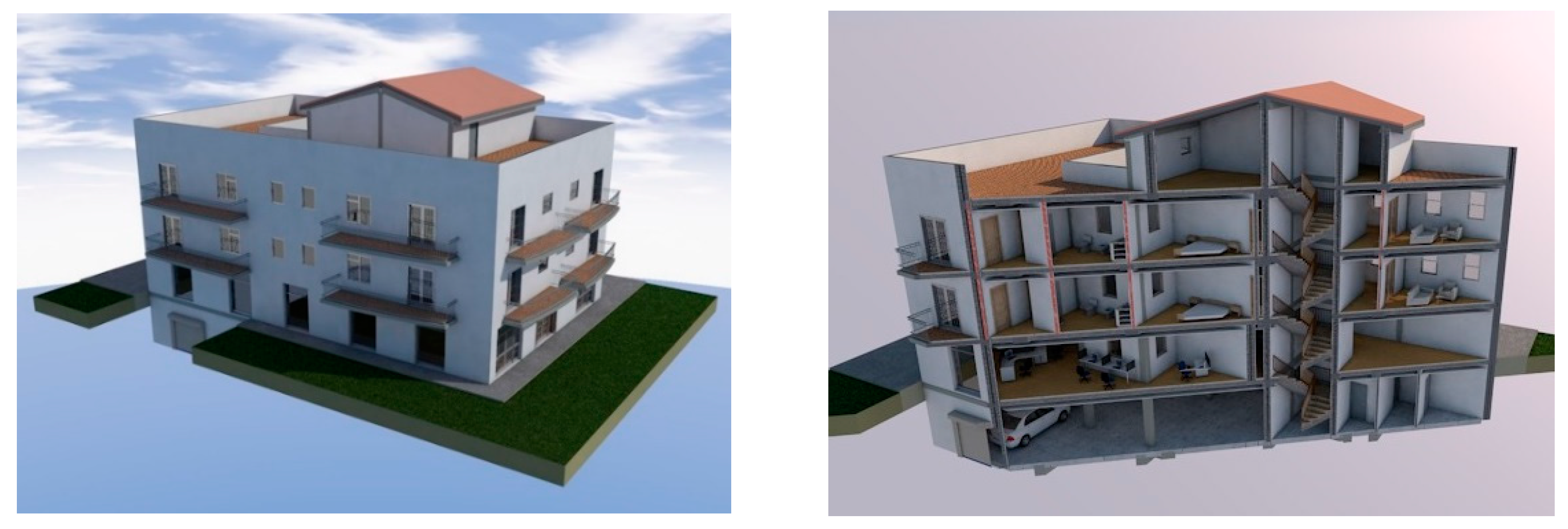
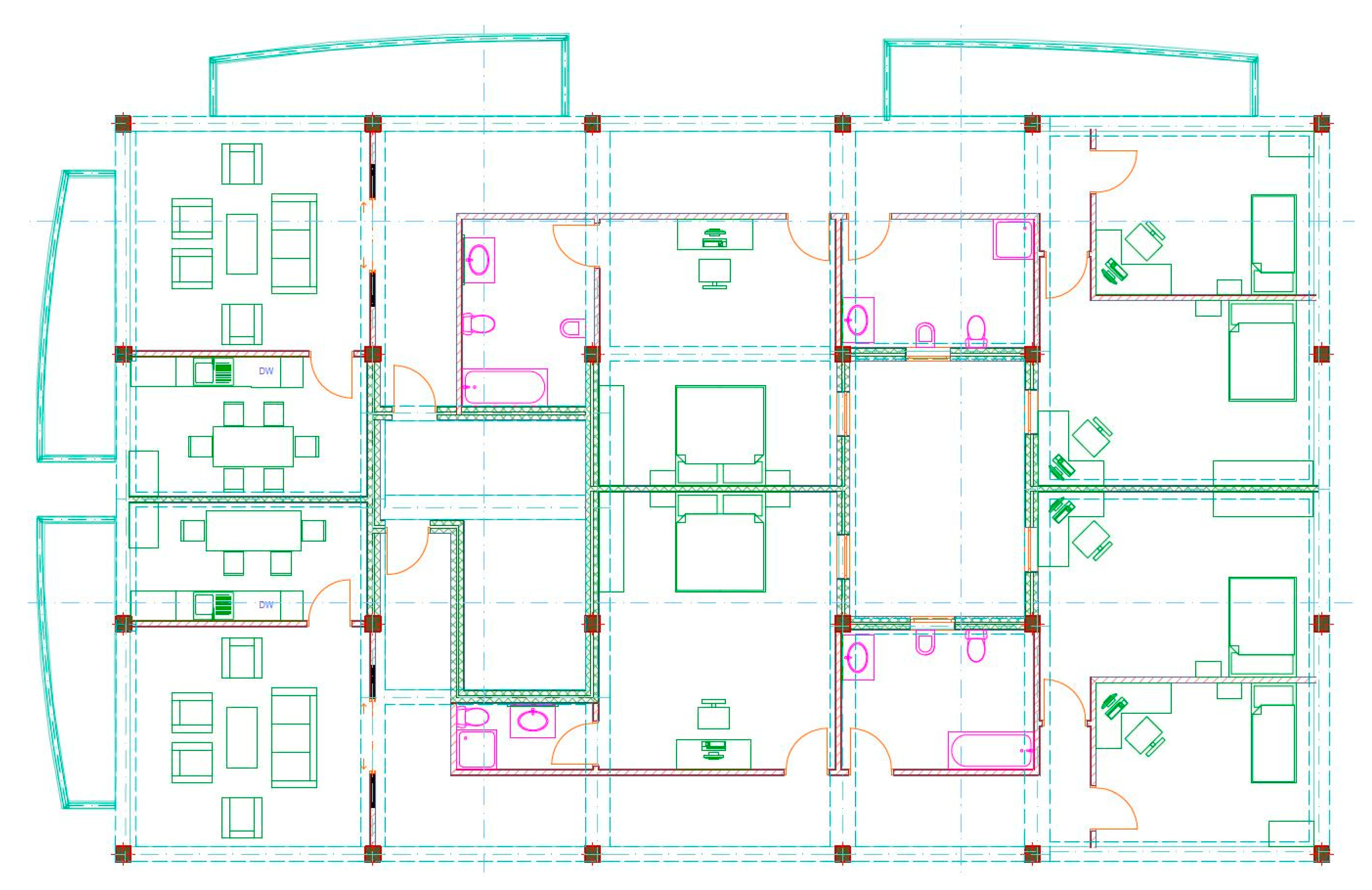
As an example of the application of the proposed method, the case of a BIM data control corresponding to the delivery of a complete project (“as built”) will be considered. This is a building with four floors (basement, F0, F1, and F2) and an attic, with garages in the basement, two commercial premises in F0, and four apartments distributed between F1 and F2—that is, two per floor. Figure 1 presents an overview of the building and Figure 2 illustrates the distribution of F1 and F2, which is the same. This section addresses three contents in relation to the application example—on the one hand, the realization of the theoretical aspects indicated above, on the other, the characterization of the case, and finally, the execution and results of the control.

5.1. Concretions of the Control

First, the aim of the control must be clear. Our interest is to verify whether the content of the BIM data file corresponds to reality, and if that reality is faithfully reflected in the data set. This is what we understand as an “as built” perspective. Thus, the completeness assessment is relevant and means that there are no excess or missing items in the BIM data. This situation means that the sampling for completeness assessment must be carried out in a way that allows both perspectives to be controlled. Thus, if this perspective were controlled exclusively from the BIM data to reality, only commission errors could be controlled, and if it were controlled from reality to the BIM data, only omission errors could be controlled. For a two-way control to be carried out, sampling should be organized in an appropriate manner, which will be proposed later.

If the populations are large, a sampling-based approach for the execution of the control is required. A sample must be representative, and therefore, extracted by simple random sampling (SRS). The SRS should be stratified to better consider the differences within a DQU. The sample will have a size that is adequate to reduce the risks (Type I and Type II errors) (see Section 3.1).

Since the completeness assessment requires both analyses—from the dataset to the reality and from the reality to the dataset—it is proposed that the sampling be executed as follows. A set of randomly distributed positions will be generated in the building; in these positions, we will locate the nearest instances bellowing to the DQU (both in reality and in the BIM data). If, for that position, the instance is the same in reality and in the BIM data, there is neither omission nor commission. If the instance of interest exists only in the BIM data or in reality, it is a commission or omission, respectively.

Once the data completeness assessment has been developed for the items that are correct (neither omissions nor commissions), the rest of the DQEs linked to the same scope can be controlled (e.g., DQEs for the metric accuracy and thematic accuracy categories). Additionally, it should be remembered that we have adopted a nonconforming items perspective (e.g., the door is right or wrong) and not a nonconformities perspective (e.g., the presence of various defects in a door).

5.2. The Case

As indicated, Figure 1 presents an overview of the building. While the reality is not known, there are BIM data that have been formed throughout the execution of the construction project—that is, the BIM data come from the design, but have received several changes and updates during the execution of the project (the construction process). Thus, as an initial hypothesis, we can consider the BIM data to be a good approximation of reality. In this way, the number of elements involved (population size estimation) in each CoI can be directly approximated (

Table 1. Categories of interest in the BIM database.

Group	Categories of Interest	Cases (N)
Elements	C1 = Doors and windows	119
	C2 = Bathrooms and Kitchens	14
	C3 = Balconies and terraces	29
	C4 = Other rooms	18
	C5 = Living rooms and bedrooms	16
	C6 = Common zones	6
	C7 = Enclosures (walls)	179
	C8 = Slabs and paving	25
	C9 = Pillars	105
	C10 = Sales unit	6
	C11 = Interior walls	200
Facilities	C12 = Electricity installation	7
	C13 = Heating and air-conditioned installations	7
	Total	731

). In this control, a significance level $\alpha =5\%$ is adopted as a Type I error for acceptance.

In relation to the DQU for the control,

Table 2. Definition of the data quality units to be considered for the control (cases for the population and sample size).

Data Quality Units	Cases in the Population (N)	Sample Size
DQU1 = Completeness of elements
DQE = Commission + omission	511
CoI = C1 + C2 + ··· + C11		50
DQU2 = Completeness of facilities
DQE = Commission + omission	182
CoI = C12 + C13		40
DQU3 = Shape Fidelity
DQE = Fidelity in shape	1605
CoI = C1 + C2 + ··· + C10		160
DQU4 = Attributes of elements
DQE = Correction of non-quantitative attributes	462
CoI = C1 + C2 + ··· + C10		50
DQU5 = Attributes of installations
DQE = Correction of non-quantitative attributes	491
CoI = C12 + C13		50
DQU6 = Shape Fidelity of walls
DQE = Fidelity in shape	200
CoI = C11		20
Total	3451	350

summarizes the configuration, population, and sample sizes. Considering the future use of this BIM dataset, the determined DQUs represent aspects of fitness whose control is considered to be relevant for use. For example, based on Table 1, the presence/absence of elements (commissions/omissions), the shape fidelity, etc., are considered relevant for the future use of this data set. This relevance is also reflected in the QLs that are established (see

Table 3. Definition of the quality controls by means of the data quality units and the conformity levels.

Quality Control	Data Quality Unit	Data Quality Measure and ID *	Conformity Level (Maximum Proportion of Defects)
QC1	DQU1	Rate of excess items (ID = 3) + Rate of missing items (ID = 7)	1%
QC2	DQU2	Rate of excess items (ID = 3) + Rate of missing items (ID = 7)	3%
QC3	DQU3	Rate of unfaithful items (ID = **)	5%
QC4	DQU4	Rate of incorrect attribute values (ID = 67)	10%
QC5	DQ5	Rate of incorrect attribute values (ID = 67)	10%
QC6	DQ6	Rate of unfaithful items (ID = **)	80%, 15%, 5% ***

(*) The ID is the identifier for this measure given in Annex D of ISO 19157. (**) This measure is not included in Annex D of ISO 19157. (***) These proportions are linked to good, acceptable, and unacceptable cases.

). From a statistical point of view, all the variables considered are of a qualitative type: Presence/absence, right/wrong, and faithful/unfaithful. The sample sizes have been set arbitrarily with the criteria set forth above (≈10%), except for the DQU2 with a larger sample size.

Prior to the control, and by agreement between the parties, QLs must be established. For this example, the specifications are those presented in Table 3. When indicating completeness, we refer to both omissions and commissions, considering both types of errors to be equivalent for error counting purposes. Finally, it should be noted that the QLs are themselves a representation of the importance of the different aspects considered in the joint control, since greater quality is demanded by the most critical elements or CoIs. Naturally, these values must be determined based on experience and the requirements of greater or lesser rigor for the BIM application. In this way, as indicated by Equation (4), the global control of the BIM data means that QC1 passed AND QC2 is passed AND QC3 is passed AND QC4 is passed AND QC5 is passed AND QC6 is passed.

5.3. Execution and Results

The execution consists of applying the steps indicated above. These steps are as follows:

• Generating random sampling positions over which the completeness control is performed.
• Performing the control by visiting the positions of the building that are part of the sampling and where the reality to BIM data and BIM data to reality perspectives are taken into account. In this step, the measurements of quantitative attributes, preferably using a laser distance meter and assessments of qualitative attributes are performed on the correct items (neither omission nor commission). This phase is very important: The data taken here are considered to be the ground truth or reference. Therefore, extreme care is required with the working methods to ensure that the captured data (qualitative and quantitative) are accurate.
• Analyzing the results and making a final acceptance/rejection decision. The defect case counts are computed (

  Table 4. Results of the defective count and p-values by quality control.

  Quality Control	Number of Nonconforming Items	Sample Size (n)	p-Value
  			Binomial	Hypergeometric	Multivariate Hypergeometric
  QC1	0	50	1.000
  QC2	5	40		0.0004
  QC3	11	160	0.179
  QC4	5	50	0.569
  QC5	2	50	0.966
  QC6	7.1 (*)	20			0.0236

  (*) The number of items per class is: 12 (good), 7 (acceptable), 1 (unacceptable).

  ). Based on these counts, and applying the functions “pbinom” and “phyper” of R [32] (indicated in the annexes), the p-values that appear in Table 4 are obtained. As can be seen, the hypergeometric model has been considered for the case QC2, and in the rest of the cases, the binomial model has been applied. Here, a MHTM is needed, so we apply Bonferroni because of its simplicity. Since α = 5% was adopted, the global null hypothesis should be rejected for any p-value less than 0.05/6 = 0.083. Given that the lowest obtained p-value is 0.0004 < 0.083, it is possible to reject the hypothesis that the BIM data complies with the specifications imposed by Table 4, since the observed data provide evidence of this.

5.4. Discussion

An example has been presented based on a relatively simple case that corresponds to a residential building. This situation limits, to some extent, the number of categories that appear and the size of the populations. Additionally, a reduced number of controls (six) have been defined. However, despite these limitations, and given that the main interest of this work is methodological, we consider that this situation is not problematic. Indeed, to present this method, we have searched for a simple and understandable case (a residential building) for most professionals and researchers working with BIM.

The presented case is a non-automatic control process because we must go to the field to carry out checks. Focusing on the statistical elements, the proposed method can be developed by any technician who has training in quality control. A researcher could use statistical programs (e.g., R) and even spreadsheets to perform the necessary statistical calculations (p-values).

We have compared the built situation (as-built) to the designed product (BIM model), but the present method is also adequate to compare a BIM model achieved through surveying and attribute collection methods to an as-is situation.

Interesting aspects, such as compliance levels, methods for measuring, sample size determination, specific details of the samples, etc., are beyond the scope of this work, as this is not an application guide. In any case, the developed example demonstrates that it is possible to work with quantitative and qualitative variables, combine variables, establish very diverse fields, use different measures, etc., and combine all these elements in a global acceptance/rejection dataset.

The present example results in the rejection of the BIM data set. In a situation with real applications, subsequent decisions will be required. For example, in ISO 2859-2, if a batch of products is rejected, those products must be repaired by the producer and will be inspected again. In our case, the decisions to be taken in the case of rejection must also be established. We could, for example, follow the same decisions as the international standards of acceptance controls (e.g., the ISO 2859 series).

One characteristic of the present method is that a single acceptance/rejection function occurs at the end, upon delivery of the building model. In some cases, a lot by lot inspection process may be of interest, like the sequential acceptance processes presented in the international standard ISO 2859-1, but solving this limitation will require further investigation.

6. Conclusions

The quality of BIM data is an issue of great importance. However, so far, it has not acquired appropriate relevance relative to the current increase in its applications. The quality of BIM data is not fully formalized, but directly applicable knowledge can be transferred from the field of geospatial data. In this paper, the framework established by ISO 19157 has been applied to BIM data due to its great similarity with geographical information.

This paper has presented the statistical basis of a method for the global quality control of BIM data with multiple DQUs, which entails different scopes and diverse DQEs. This method has a valid, affordable, and known statistical formulation, as it is based on the known distribution functions that are applied in the field of quality control. The main contributions of this work are two-fold. First, we present a proposal and example of using the ISO 19157 data quality framework for BIM data; second, we use a statistical approach formulation, including an example of how to handle the joint control of several types of errors, each with different quality specifications.

An example of application in a residential building case has been presented. This case uses BIM data of a medium to small size, but represents a very common type of construction. The control developed corresponds to the “as built” perspective—that is, to ensure that the content of the BIM data is a true reflection of reality. An “as built” control is a more complex control than a control based on performing logical check routines on the BIM data, since an “as built” control requires probabilistic sampling. The present example has been developed considering six quality controls, which entails the definition of five DQUs and QLs. The final joint result of the control has been rejected. The definition of the DQU and QL are issues adaptable to each situation and use case.

We consider the application of the proposed method to be affordable for experts based on its quality compared to a conventional statistical framework. The present method is simple, both in its statistical elements (very similar to conventional acceptance testing in industry, for which examples of the functions to be applied in the R program environment are provided [32] R Core Team, 2019), and in terms of its execution, for which we have presented an application example and explained the most relevant issues.

We believe that the method presented here may serve as the basis for the development of BIM data quality controls with an “as built” perspective, but could also be adapted to other perspectives. An interesting future advance would entail the proposal of DQUs and QL based on this method by some professional organizations or regulatory bodies of the building sector. Additionally, statistical control requirements should be established for BIM data deliveries in legal regulations.