Optimized Location-Allocation of Earthquake Relief Centers Using PSO and ACO, Complemented by GIS, Clustering, and TOPSIS

Abstract

After an earthquake, it is required to establish temporary relief centers in order to help the victims. Selection of proper sites for these centers has a significant effect on the processes of urban disaster management. In this paper, the location and allocation of relief centers in district 1 of Tehran are carried out using Geospatial Information System (GIS), the Technique for Order of Preference by Similarity to Ideal Solution (TOPSIS) decision model, a simple clustering method and the two meta-heuristic algorithms of Particle Swarm Optimization (PSO) and Ant Colony Optimization (ACO). First, using TOPSIS, the proposed clustering method and GIS analysis tools, sites satisfying initial conditions with adequate distribution in the area are chosen. Then, the selection of proper centers and the allocation of parcels to them are modelled as a location/allocation problem, which is solved using the meta-heuristic optimization algorithms. Also, in this research, PSO and ACO are compared using different criteria. The implementation results show the general adequacy of TOPSIS, the clustering method, and the optimization algorithms. This is an appropriate approach to solve such complex site selection and allocation problems. In view of the assessment results, the PSO finds better answers, converges faster, and shows higher consistency than the ACO.

1. Introduction

Most of the world’s population lives in areas prone to natural disasters [1]. Iran is located in a seismically active region with relatively high records of earthquakes [2]. Earthquakes often result in severe human loss and intensive economic and social problems [3].

Recent studies on disaster management concentrate on damage possibility as well as the responses to disaster [4]. Planning for response to different natural disasters, including earthquake, has become an important aspect of urban management. From the moment of an earthquake’s occurrence, relief is necessary to respond to the damages. This includes all the measures which are put into action in order to rescue human lives, to maintain property, and to lessen the effects of the disaster. Providing appropriate places to establish relief centers after an earthquake is one of the most important decisions in disaster management and relief planning.

Site selection of service centers is essentially a location-allocation problem, which consists of two elements: The location part means where the facilities should be settled; the allocation part means what customers or requests are to be served by each facility center [5,6,7]. The procedure should provide the best distribution of the centers and allocate all parcels to their closest possible centers. This makes the location-allocation a complex optimization problem [8]. The first cause of complexity is the computationally expensive objective function, which is the total distance of the centers from their allocated parcels. The second reason for the complexity is the width of the search space: Considering the number of candidate sites among which the centers are to be selected, and the large number of possible combinations for the allocation of parcels to centers, the search space is in fact very wide. Solving such a complex problem using mathematical and direct methods is usually very time-consuming. Instead, meta-heuristic methods can find solutions close enough to the real optimum solution, in a reasonable time.

The goal of this study is to use and compare the applicability of PSO and ACO meta-heuristic algorithms for the location-allocation of the relief centers in district 1 of Tehran. To achieve this goal, first of all, the sites having the best initial conditions with adequate distribution in space are chosen, using GIS, the TOPSIS decision making model and a proposed simple clustering method. The main reason for this is to reduce the search space to a limited number of candidate sites. Then, the final centers are selected and parcels are allocated to them using PSO and ACO meta-heuristic algorithms. This is an appropriate approach to solving such complex site selection and allocation problems. Also, in this research, PSO and ACO are compared using different criteria. In the existing literature, no comparison can be seen using these two algorithms for the location-allocation of relief centers.

The first section of this paper introduces the research problem and objectives. The second section reviews the relevant previous research. The basic concepts of PSO, ACO and TOPSIS are described in Section 3. In Section 4, the used methods are briefly presented. This section also introduces the study area and data. In the next section, the implementation steps and results are briefly presented. Finally, conclusion and some suggestions for the continuation of the research are provided in Section 6.

2. Previous Work

2.1. Optimized Location-Allocation of Relief Centers

Due to the importance of the subject, many studies are done on determining the location of the relief centers. Beraldi and Bruni [9] presented a probabilistic model to optimally locate the relief facilities in an uncertain environment. Tzeng, Cheng [10] suggested an exact multi-dimensional model to allocate the relief items to the affected places considering cost, response time and accountability. Balcik and Beamon [11] developed a model to determine the number and position of distribution centers in a relief network, along with the amount of relief items that are to be saved in each distribution center. Hooshangi and Alesheikh [12] presented an approach to improving the task allocation in disaster environments. Mingang, Zeng [13] used a two-stage heuristic algorithm to solve the emergency facilities location problem and emergency resource routing problem. The goal was to minimize the total costs.

2.2. Meta-Heuristic Algorithms

To overcome the limitations of traditional approaches, meta-heuristic algorithms are developed as part of artificial intelligence techniques. They have the ability to solve complex optimization problems in wide and many-dimensional search spaces. Artificial intelligence techniques are widely used and considered in many computing research [14,15]. In a paper by Yi and Kumar [16], provision of the facilities is divided into two phases of determining the vehicle routes and dispatching the relief commodity, which are optimized using the ACO algorithm. Sheu [17] used a phase clustering optimization model for the distribution of emergency facilities. Ohlemüller [18] implemented and compared the two algorithms of Tabu search (TS) and Simulated Annealing (SA) for the linear version of the problem. Brimberg, Hansen [19] compared the capabilities of the Genetic Algorithm (GA), TS and Variable Neighborhood Search (VNS) for the same matter. Zheng, Chen [20] divided the disaster relief operations problems into five classes of general transportation planning problems, facility location problems, routing problems, roadway repair problems and integrated problems. They described the applications of Evolutionary Algorithms (EAs) including GA, PSO and ACO in any of those classes. Similarly, Li, Zhao [21] reviewed the applications of optimization techniques, including meta-heuristics, to the location and planning of emergency response facilities.

So far, various meta-heuristic algorithms are successfully used to solve spatial problems related to disaster management. Yet, continuously new optimization algorithms are developed and proposed (such as Dragonfly algorithm [22], Crow search algorithm [23], the whale optimization algorithm [24], Stochastic fractal search [25], etc.). According to literature, ACO and PSO algorithms are among the most important and popular algorithms used in disaster management and allocation problems. Authors of [16,26,27,28,29,30] used and evaluated PSO and ACO for disaster management. Similarly, Hu, Xu [31] used a modified version of PSO for the allocation of earthquake emergency shelters. In addition, the authors of [6,32,33,34,35,36,37,38,39,40] showed the adequacy of PSO and ACO for the location-allocation related problems. The authors of [41,42,43,44,45,46,47] used PSO, ACO and other algorithms, for some applications different from location-allocation. The results of comparisons were not similar for different applications. Vilovic, Burum [48] and Adrian, Utamima [49] performed similar comparison for applications far different from relief centers. Vilovic, Burum [48] used the two algorithms for the location of WLAN base stations, gaining better results for PSO, whereas, Adrian, Utamima [49] used these algorithms along with GA for optimization of construction site layout. The results showed higher levels of effectiveness for PSO and higher levels of efficiency for ACO.

Considering different results reported in previous work, and their applications, which are different from the location-allocation of relief centers, their results cannot be directly compared with the present research. As mentioned, the characteristic goal of the present study is to compare the capabilities of PSO and ACO meta-heuristic algorithms for the location-allocation of earthquake relief centers.

Saeidian, Mesgari [8] emphasize the necessity of allocating relief centers to the parcels, instead of city blocks. In addition, they recommended the use of multi-criteria decision making methods for filtering and initial selection of relief centers. Therefore, in this study, relief centers are allocated to the parcels. Besides, a proposed clustering method and TOPSIS are used for the initial site selection of the relief centers. Moreover, some further parameters recommended by [8] are considered here. Finally, in this paper, two algorithms of PSO and ACO are used and compared, for the following reasons:

• Although PSO is essentially used for problems with continuous search space, some researchers proposed discrete versions of PSO for discrete location/allocation problems [50,51,52,53]. Therefore, comparison of the adequacy of a discrete PSO with ACO, for the location-allocation of relief center, was raised as the research question of the present study.
• As mentioned earlier, these two algorithms are frequently used for location-allocation problems. However, they are rarely compared when used for such issues. In addition, the results obtained for one application cannot be simply generalized to other applications [54]. As shown in the reviewed literature, no comparison has been made regarding these two algorithms for the location-allocation of relief centers. Therefore, in the present research, these two algorithms are used and compared for the considered new application.

3. Theoretical Background

PSO, ACO and TOPSIS are the main algorithms and methods used in this research. Their basic concepts are explained in the following.

3.1. Swarm Intelligence Algorithm

Swarm Intelligence (SI) is a branch of artificial intelligence. It consists of algorithms inspired by the collective behavior of the decentralized self-organized agents [55]. Although these agents have simple performances and do not follow a central control system, their simple interaction results in a complex behavior of the whole system. The most popular SI algorithms are ACO [56], PSO [57,58] and Bee algorithms [59]. As mentioned, PSO and ACO were selected in this research. Their main concepts are briefly described in this section.

3.1.1. PSO Algorithm

The idea of the PSO algorithm was proposed and developed gradually by different researchers [57,60,61,62,63]. The algorithm is inspired by the swarm movement of birds, fish and insects. The fame of Particle swarm is because of its simplicity. This algorithm, like many other population-based algorithms, is based on the communications among certain elements. These elements are moving toward the positions in space having higher optimization functions. Every particle has a memory, and its movement is a combination of its current movement, the movement toward the best position the particle has ever seen (Personal Best (PB)), and the movement toward the best positions found by other particles (Global Best (GB)) [63].

In PSO, every particle i has a position x_i (representing a solution to the problem at hand) and a velocity v_i (velocity indicates the movement of a particle from a position to another), which are updated in every repetition. The velocity is calculated by Equation (1) [63].

$${\overrightarrow{v}}_i=w{\overrightarrow{v}}_i+c_1{\overrightarrow{\phi }}_{1i}({\overrightarrow{p}}_i-{\overrightarrow{x}}_i)+c_2{\overrightarrow{\phi }}_{2i}\left({\overrightarrow{p}}_g-{\overrightarrow{x}}_i\right),$$

(1)

In the above equation, w is the inertia weight, p_i is the PB of particle and p_g is the GB. The Φ₁ and Φ₂ weights in each step are randomly selected for the particles. c₁ and c₂ are constant positive parameters which are called acceleration coefficients (they determine the maximum value of steps the particles can take). Inertia weight w controls the impacts of the previous velocity [64]. The position of each particle in every step is updated by adding the calculated velocity vector to its position vector (Equation (2)) [63].

$${\overrightarrow{x}}_i={\overrightarrow{x}}_i+{\overrightarrow{v}}_i,$$

(2)

The appropriate choice of inertia weight and acceleration coefficients brings a balance between universal exploration and local exploitation [60,64,65]. The PSO algorithm consists of the following 5 steps [62,63].

• For each particle, making an x position vector and a v velocity vector randomly.
• Assessing the goodness of all particles using an optimization function.
• Updating the best position found by each particle and the best position found so far by the group.
• Updating the velocity and position of each particle using Equations (1) and (2).
• Repeating stages 2 to 4 until reaching the stop condition.

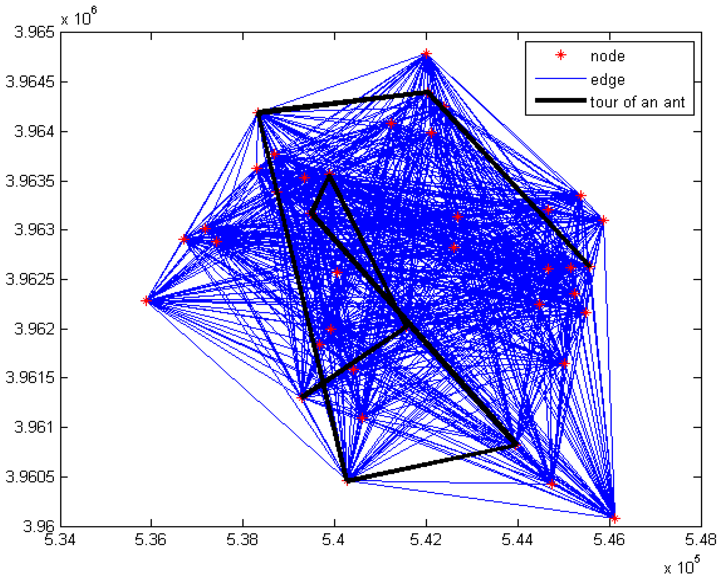
3.1.2. ACO Algorithm

The ACO algorithm is used to solve a wide range of optimization problems [6,56,66,67], in which, a solution is in fact the sequential selection of values for a set of ordered parameters. In other words, a solution (ant) is constructed by initializing all parameters in order (Construct Ant Solution). After constructing all required ants, their objective function values are calculated. Some of the best ants are selected based on their objective functions values. For such a selected ant, the pheromone or bonus of optimality is calculated based on its objective function value. This pheromone is given to the ant (solution) components, i.e., to the relevant values of parameters (update Pheromones). An ant of the next generation chooses the available parameter values with possibilities proportional to their pheromones. The next generation ants are better than the previous ones because they use the experience of the previous ants. In the meantime, around each constructed ant (solution), a local search is done optionally (Apply local search) [6,66,67,68]. The pseudo-code of the ACO algorithm is presented in Algorithm 1.

Algorithm 1 ACO meta-heuristic [68]

Set parameters, initialize pheromone trails

while termination conditions not met do

ConstructAntSolutions

ApplyLocalSearch  [optional]

UpdatePheromones

end while

The steps of the ACO algorithm are [6,66,67,68]:

• Initialize the parameters (pheromone, etc.);
• Insert the origin city for each ant in its forbidden list, in order to prevent it from going back that city;
• Calculate the probability of selecting the next city, at each city, for any ant;
• Adjust the population of cities for the selection of each ant to the forbidden list of the ant;
• Add the selected city of each ant to its forbidden list;
• Determine the best path;
• Update pheromones based on the path quality;
• Evaporate the pheromone;
• Go to step 3 (if the stop condition is not met).

3.2. TOPSIS

In recent decades, Multi-Criteria Decision Models or Methods (MCDM), such as TOPSIS, have attracted the attention of many researchers. In the TOPSIS method, m alternatives are assessed by n criteria, so each problem could be considered as a geometrical system including m points in an n-dimension space. This technique is constructed based on the concept that the selected alternative should have the shortest possible distance to the positive ideal solution (A_i⁺) and the longest distance to the negative ideal solutions (A_i⁻). The TOPSIS method requires the following steps [69]:

• Establishing a decision matrix
• Calculating the normalized decision matrix
• Calculating the weighted normalized decision matrix
• Determining the positive and negative ideal solutions
• Calculating the distances through Euclidean norm
• Calculating the relative closeness to the ideal solution
• Ranking the alternative

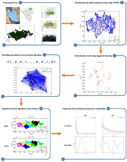
4. Data and Methodology

The main stages and activities of this study and their sequence are represented in Figure 1.

Considering the requirements of the used methods, the data were collected and prepared. Then, the centers were selected in two stages. In the first stage, TOPSIS and the proposed clustering method were used to prioritize the sites and to choose centers with higher priority and an appropriate distribution in the district. Then, meta-heuristic algorithms were used to choose the final centers. The performance of these algorithms for the data of district 1 of Tehran is compared and explained in the following sections.

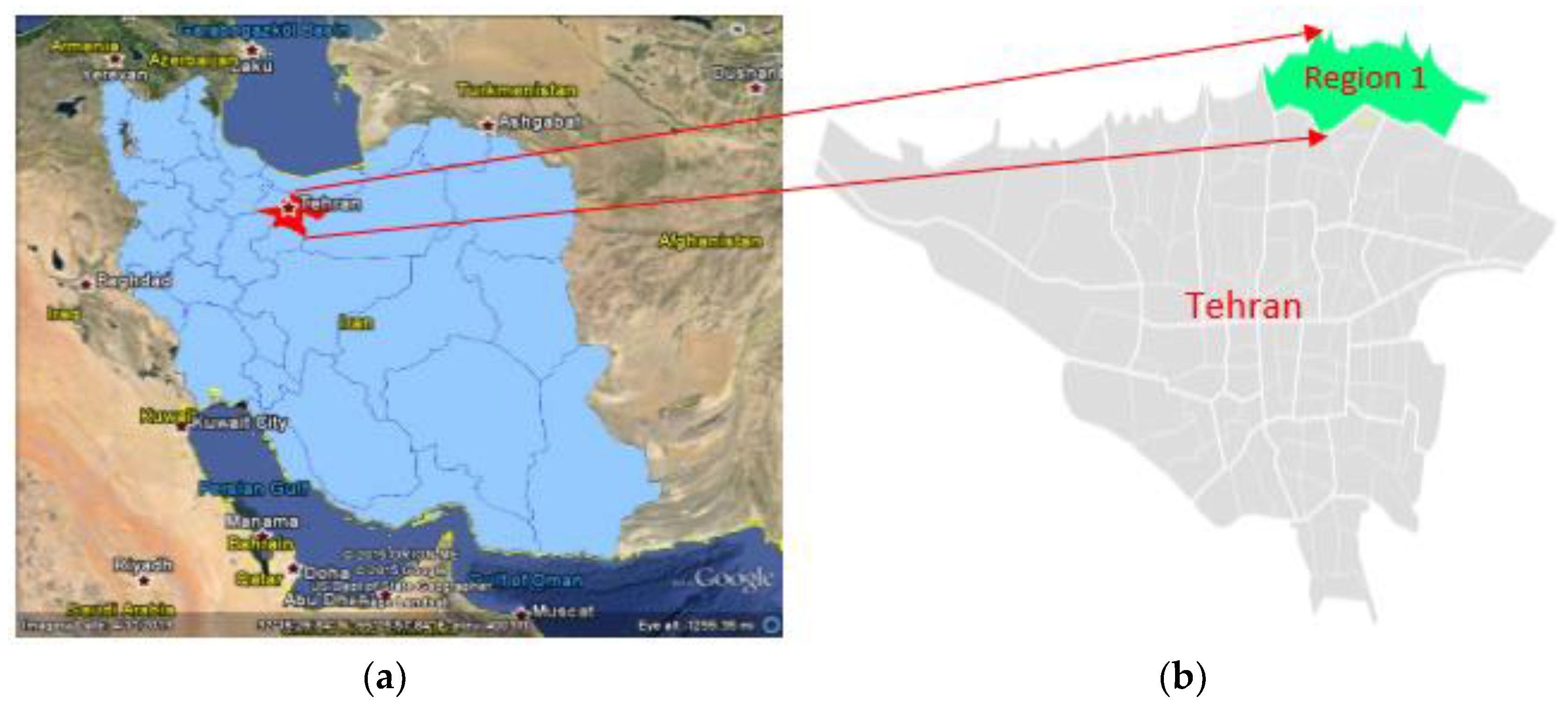
4.1. Application Site

Tehran is an earthquake-prone city with many active fault lines. On the other hand, it is both the political and socio-economic capital of the country. Therefore, district (region) one of Tehran was chosen for the case study, which is close to the fault line of north of Tehran [70]. The position of district 1 in Tehran is shown in Figure 2.

4.2. Data Collection

Data collection and compilation are among the most essential steps in various applications [72,73]. In this stage, all the required data (spatial and non-spatial) were collected. This includes the maps of parcels, fault lines, routes, slope, land use, and urban blocks, along with the area and population information of the blocks. All the required data were collected from the “Ministry of Roads and Urban Development” and their quality were sufficient for the implementation of this research.

4.3. Data Preparation

In this research, GIS was used for the preparation and analyses of the spatial data. In this research, each parcel was supposed to be allocated to its closest relief center. The gravity centers were calculated for the polygons of parcels and the relief centers, using GIS functions. These points were considered as the representatives of the respective polygons. Then, the geographical coordinates of these points were saved in an appropriate format to be entered into the meta-heuristic algorithms.

4.4. Important Parameters in Relief Centers Allocation

As discussed earlier, many parameters can be considered for the selection of the appropriate relief centers from the view point of a disaster relief manager. However, because of the research limitation, such as the availability of the data, the following parameters were considered:

• present land use of the relief centers
• area of the relief centers
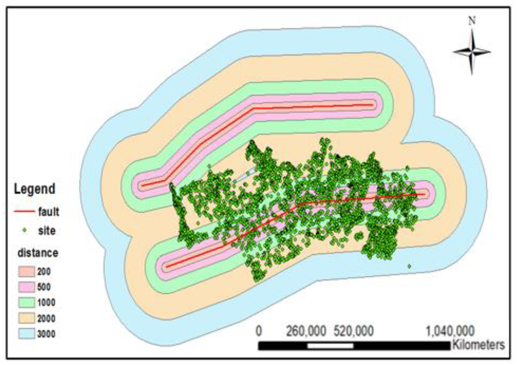
• distance of the relief center from the fault lines
• population
• slope of the relief center
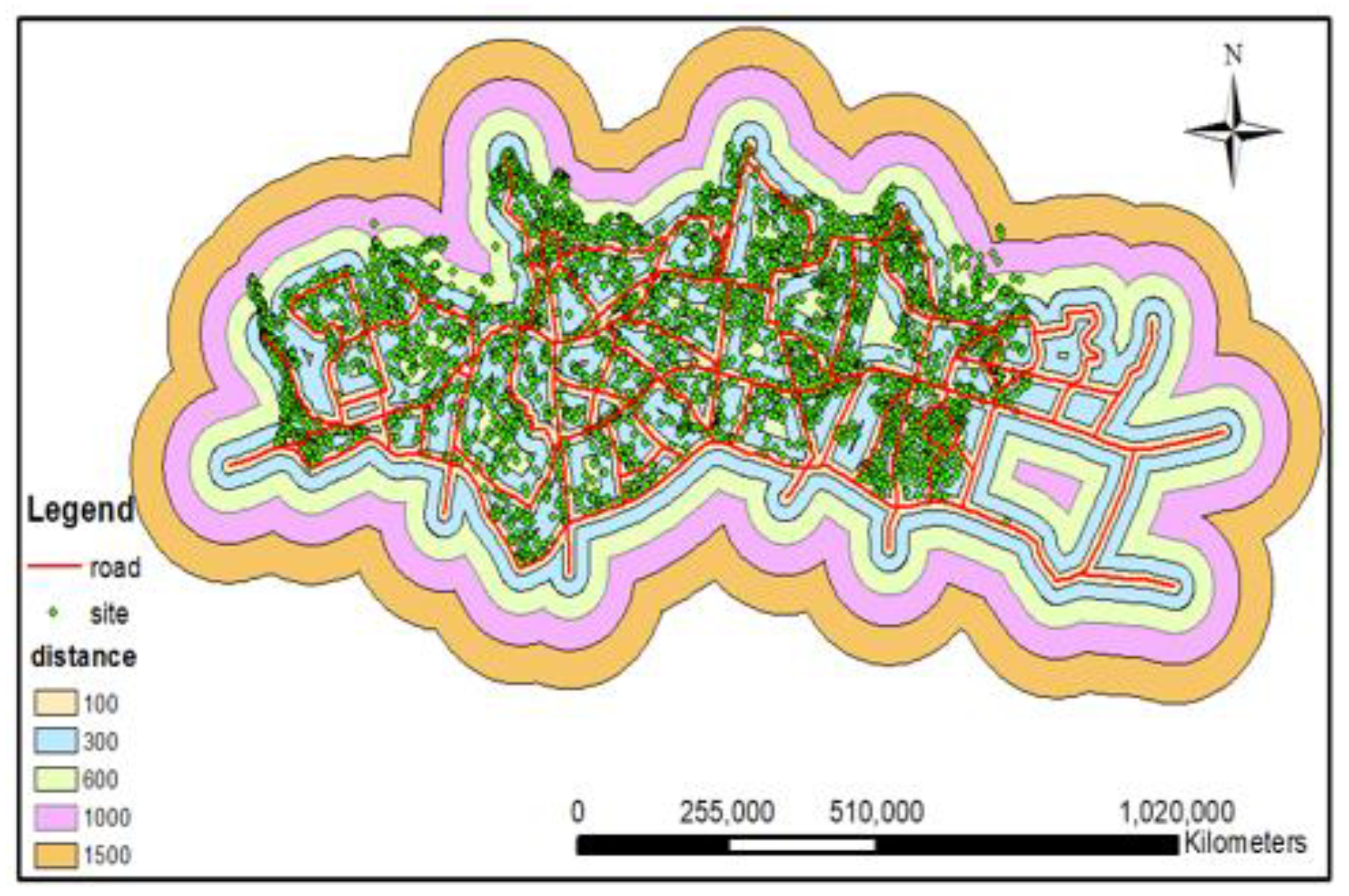
• distance of the relief centers from the routes
• distance of the relief centers from each other
• distance of the parcels from the relief centers

The first six parameters were used by the TOPSIS method for the initial selection of centers. The distance of the relief centers from each other was considered by the proposed clustering method to exclude the sites close to each other. This parameter was supposed to be minimized by the meta-heuristic algorithm. The reason for this stepwise approach was that considering all parameters directly in the optimization process would have resulted in much higher levels of complexity.

In the following, the way each parameter is dealt with is briefly discussed.

● Land use

In this research, it is assumed that open and recreational spaces, unconstructed lands, parks, gardens and villas, and parking lots are suitable for temporary relief center, as they normally have more open space and less constructed parts. To use the land use type in decision modeling, a suitability score, between one and five, is given to each land use type by experts. Higher scores mean better land use types. The scores given by experts to the mentioned land use types are 4, 5, 3, 1 and 2 respectively.

● Area

The more area a site has, the more appropriate it is for the establishment of temporary relief centers after the earthquake.

● Distance from the fault

Considering the damages caused by the earthquake, the relief centers far from existing fault lines are preferred. The distance buffers from the fault lines are shown in Figure 3.

● Population around a site

Relief centers should be preferably established in more populated areas. For each site, the blocks inside a one-kilometer buffer of the site were selected. Then, the population summation of these block was allocated to the sites and considered as the population around the site.

● Slope

The raster slope map of the area was transferred to point features using GIS. Then the slope of the nearest point to each site was considered as its slope.

● The distance of centers from the main routes

The distance of centers from the main routes of district 1 was calculated using GIS and was considered as one of the selection parameters. The distance from the routes, shown as buffers, is represented in Figure 4.

● Distance of the relief centers from each other

It is not appropriate to select relief centers in the vicinity of each other. This parameter was taken into account by the proposed clustering method, as described in Section 4.7.

● Distance of the relief centers from parcels

The parcels are supposed to be mostly allocated to their closest centers. Therefore, centers should be selected such that the sum of their distances from the parcels allocated to them is minimized. This parameter was entered into the PSO and ACO algorithms as an objective function.

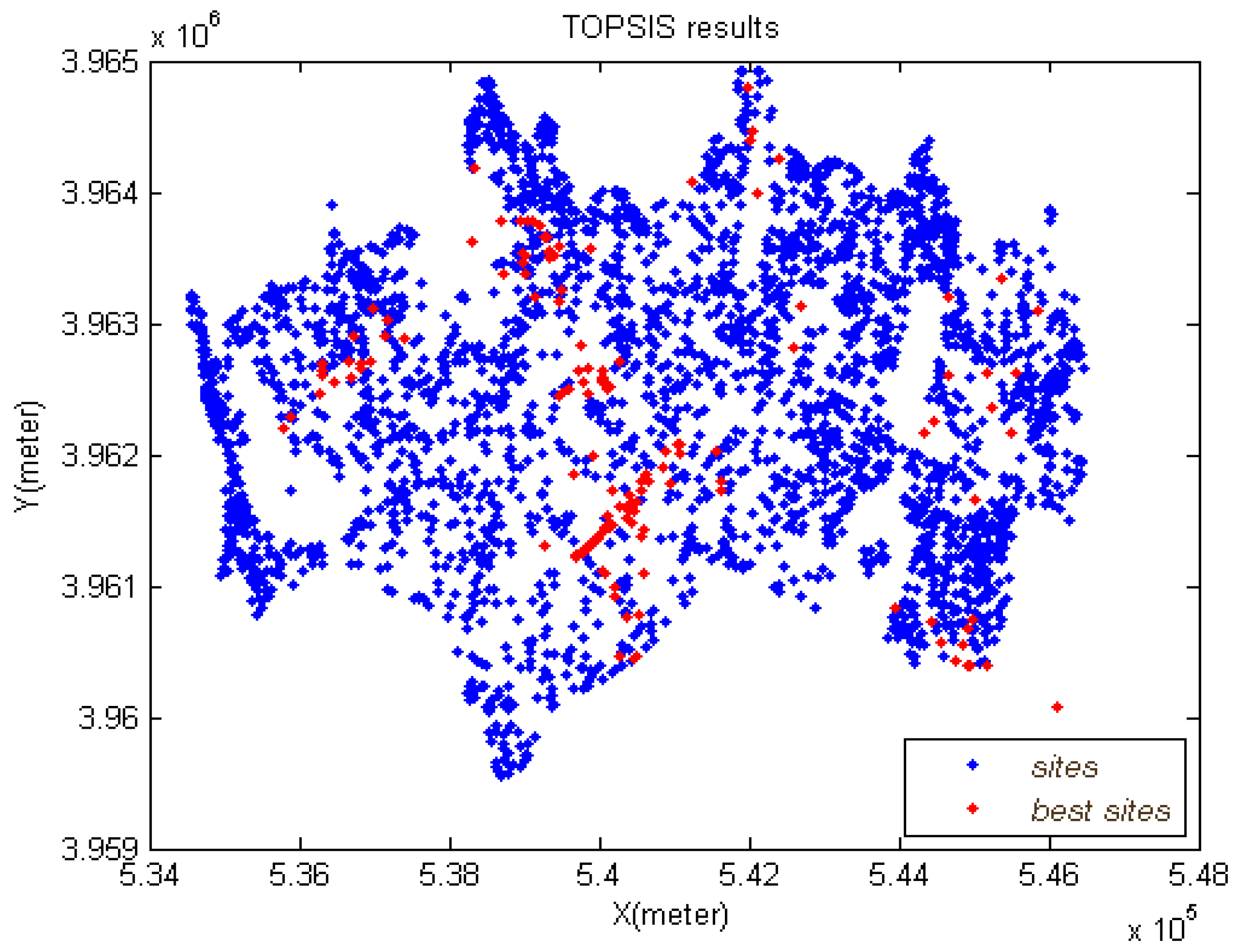
4.5. TOPSIS Implementation

The purpose of this stage is to rank the available 3065 sites according to the first six parameters. Many methods have already been suggested for multi-criteria decision making. Among the most famous methods are AHP (Analytic Hierarchy Process), TOPSIS and VICOR. In this paper, because of the high number of alternatives, AHP and VICOR could not be used. Thus, the TOPSIS method is chosen to be used.

First of all, the decision matrix and weight of each one should be determined. In

Table 1. Decision matrix and weight of criteria.

Wi	0.25	0.15	0.2	0.2	0.05	0.15
Criteria	Land Use Score (C1)	Area (C2)	Distance from Fault (C3)	Population (C4)	Slope (C5)	Istance from Road (C6)
Altern.
1	3	2495.900	1302.500	2799	6.086	73.463
2	3	31.700	1289.880	3279	10.133	265.751
3	3	207.400	1301.798	2799	6.086	49.904
…	…	…	…	…	…	….
3065	5	3991.800	1034.640	9439	10.948	58.597

, decision matrix and weight of criteria are presented. MCDM problems usually include multiple criteria. Determining the relative importance of these criteria, from the decision makers’ point of view, is called criteria weighting. Many methods, such as Direct Rating, Ranking Method, Point Allocation, are already proposed for criteria weighting [74,75]. In this research, considering its simplicity, the point allocation approach is used. In this method, the decision maker divides 100 points among the assumed criteria. The counts of points given to a criterion defines its relative importance. The summation of points given to all criteria should be 100. After the allocation of points, the weights of the criteria are transferred to the 0-1 range [74,75]. In this article, the weights of criteria, related to the site selection of relief centers, are defined by a single disaster-management expert, using the point allocation method.

In this study, criteria of land use (C1), area (C2), distance from the fault lines (C3) and population (C4) are positive; and slope (C5) and distance from the routes (C6) are negative criteria. In TOPSIS, alternatives with larger relative closeness (CL) values, the relative closeness to the ideal solution, are better [69]. In

Table 2. Alternatives ranking.

Rank	Altern.	CL
1	209	0.92239
2	20	0.66403
3	1522	0.22652
4	2547	0.22043
5	842	0.20619
6	77	0.18900
7	283	0.18603
…		…
3059	934	0.06885
3060	773	0.06737
3061	939	0.06434
3062	387	0.05200
3063	447	0.05143
3064	395	0.05142
3065	405	0.05141

, ranking of alternatives is presented based on TOPSIS. By ranking of 3065 alternatives (Table 2), 150 choices having higher priorities were chosen and entered to the next step as input. The position of these sites amongst other sites is shown in Figure 5.

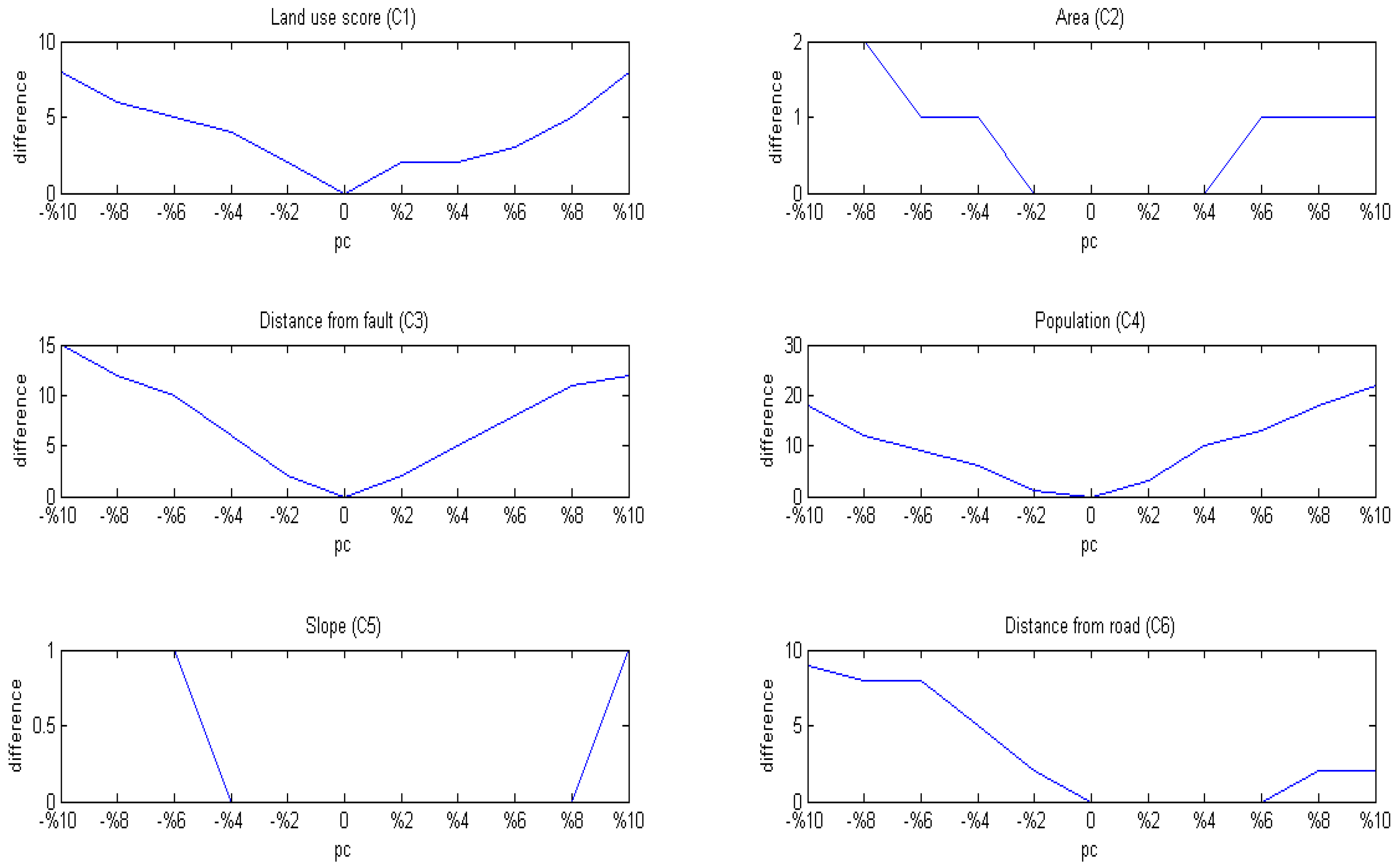
4.6. Sensitivity Analyses

In the TOPSIS method, an important factor in ranking is the criteria weights. Sensitivity analyses can be used to determine the effect of criteria-weights on the TOPSIS ranking. In sensitivity analyses, we defined how much a criterion-weight can be changed without changing the results. In other words, what ranges of a criterion-weight can generate similar results. Having determined such ranges, the sensitivity of the results to different criteria can be defined.

Many methods of sensitivity analyses are available. A popular and simple method is “One at a Time (OAT) method. In OAT, each input factor is changed at a time and its effect on the output is observed, while holding all other factors stable [76]. To start the process, three variables should be defined: the changeable factor, range of percent change (RPC), and increment of percent change (IPC).

In this research, the RPC and IPC were set to ±10% and ±2%, respectively, for all criteria-weights. The result of TOPSIS of 150 sites were selected for earthquake relief centers. The re-emergence of these sites is considered as the base of sensitivity analyses. In other words, the two sets of 150 sites resulted from TOPSIS, before and after changing a criterion-weight, were compared. The count of altered sites is assumed as the sensitivity of TOPSIS to that criterion. Figure 6 shows the count of sites changed due to the changes made in each criterion-weight. The horizontal axis shows the number of changes made to each criterion-weight, and the vertical axis is the count of consequently altered sites.

As shown in Figure 6, the model result is hardly sensitive to the weights of slope and area criteria. That is, changes in the weight of these criteria result in small changes in the 150 selected centers. Thus, the variation between (−4%)–(+8%) on the slope weight, did not change any of the 150 selected centers. After these two, the least sensitivity is related to the distance-from-road criterion weight. The change in the results is very small for a 10% change in that weight and is low for a −10% change in that weight. Having the changes of (−10%)–(+10%) in the slope and area weights, only one and two centers will be changed, respectively. The results (150 selected centers) are more sensitive to the weights of the population and distance from the fault lines. With a 10 percent change in the population and distance-from-faults criteria weights, the number of changed centers will be 20 and 15, respectively. The next most important criterion is the land use. Finally, according to Figure 6, the order of sensitivity of the results to the criteria weights from the highest to the lowest are: population (C4), distance-from-faults (C3), land use (C1), distance-from-road (C6), area (C2) and slope (C5).

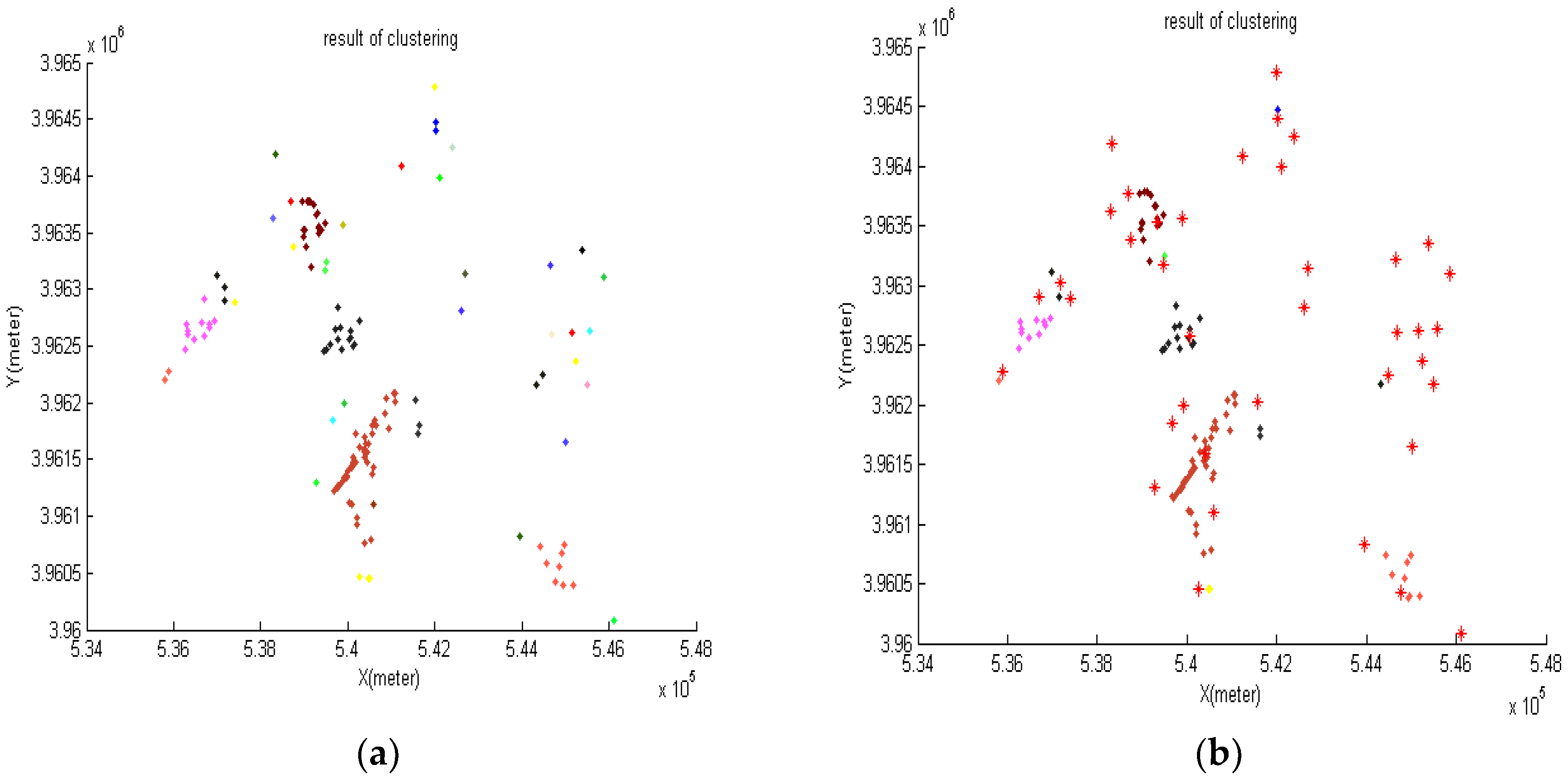
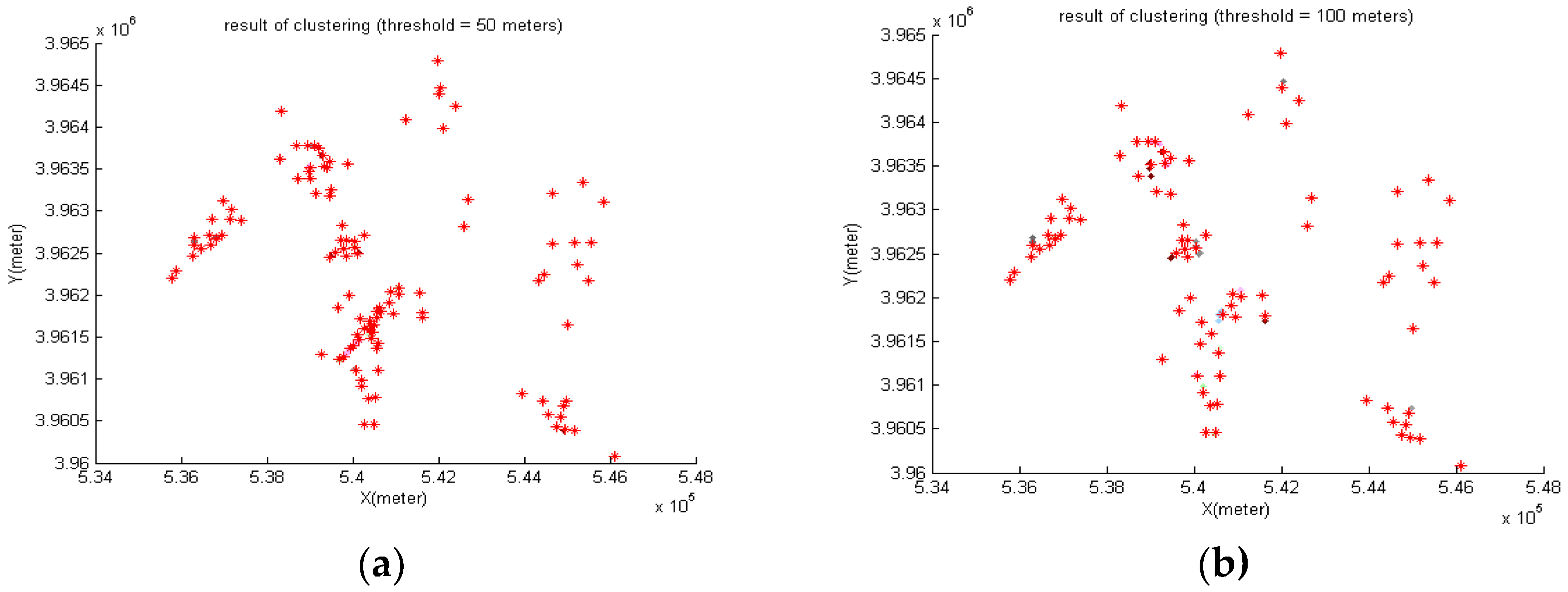
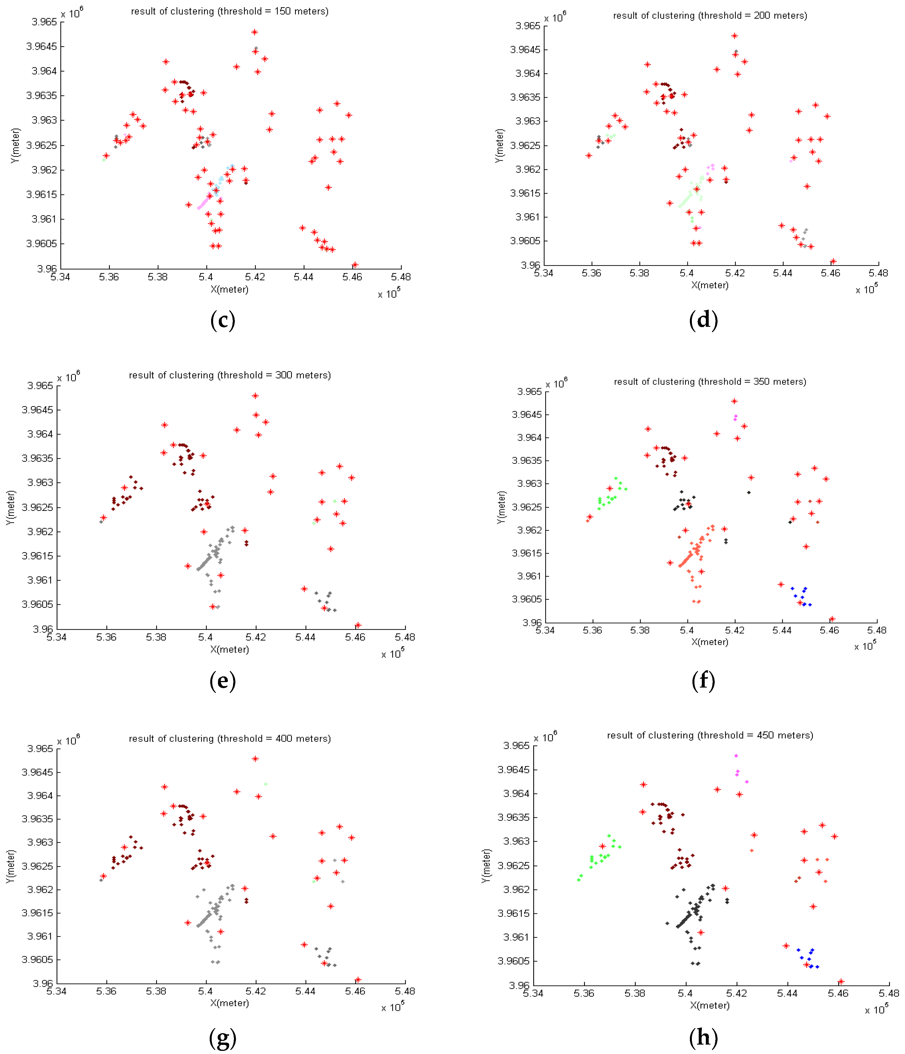
4.7. Reducing the Density of Sites by Clustering

As can be seen in Figure 5, many of the 150 sites are too close to each other. Many of them are so close that selecting any of them would be equivalent with regard to the allocation problem. In other words, having them all in the optimization process would merely increases the calculations. Therefore, clustering is carried out based on distance. Then, in each cluster, the alternative with the highest TOPSIS rank is kept as the representative of that cluster and the rest is removed. The following are the main steps of this process.

• Proximity threshold (limit) is determined.
• Every site is placed in a cluster.
• The distances between all sites are calculated, and if two sites are closer than the threshold, their clusters are merged.
• Clusters having a common site are merged.
• In each cluster, the site having higher TOPSIS rank is kept and the rest are removed.

In this research, the value of the threshold is determined as 250 m by trial and error. In Figure 7, the clustering carried out with this threshold and the final centers achieved by clustering are shown.

As mentioned previously, the output of TOPSIS was 150 candidate sites, many of which are too close to each other. This causes heavy calculations in the next stage. The number of candidate sites should be reduced by clustering. The clustering threshold has a strong effect on the number and spatial distribution of clusters. In this research, this threshold is set to 250 meters, using trial and error. This results in the 39 cluster centers, from which 9 centers with proper spatial distribution are to be selected by optimization.

Having small thresholds will result in the creation of many adjacent clusters. Setting the threshold to 50, 100, 150 and 200 meters creates 112, 83, 63 and 54 cluster centers, respectively. Having so many clusters, the objective of clustering, which is the removal of close centers, is not achieved. On the other hand, higher thresholds such as 300, 350, 400 and 450 meters result in the creation of 31, 27, 25 and 17 cluster centers, respectively. With a few clusters, many distant centers will fall in the same cluster and will be removed. This results in improper spatial distribution of centers, such that some parts of the space are not covered by any center. Figure 8 shows the counts and distribution of cluster centers resulting from different thresholds.

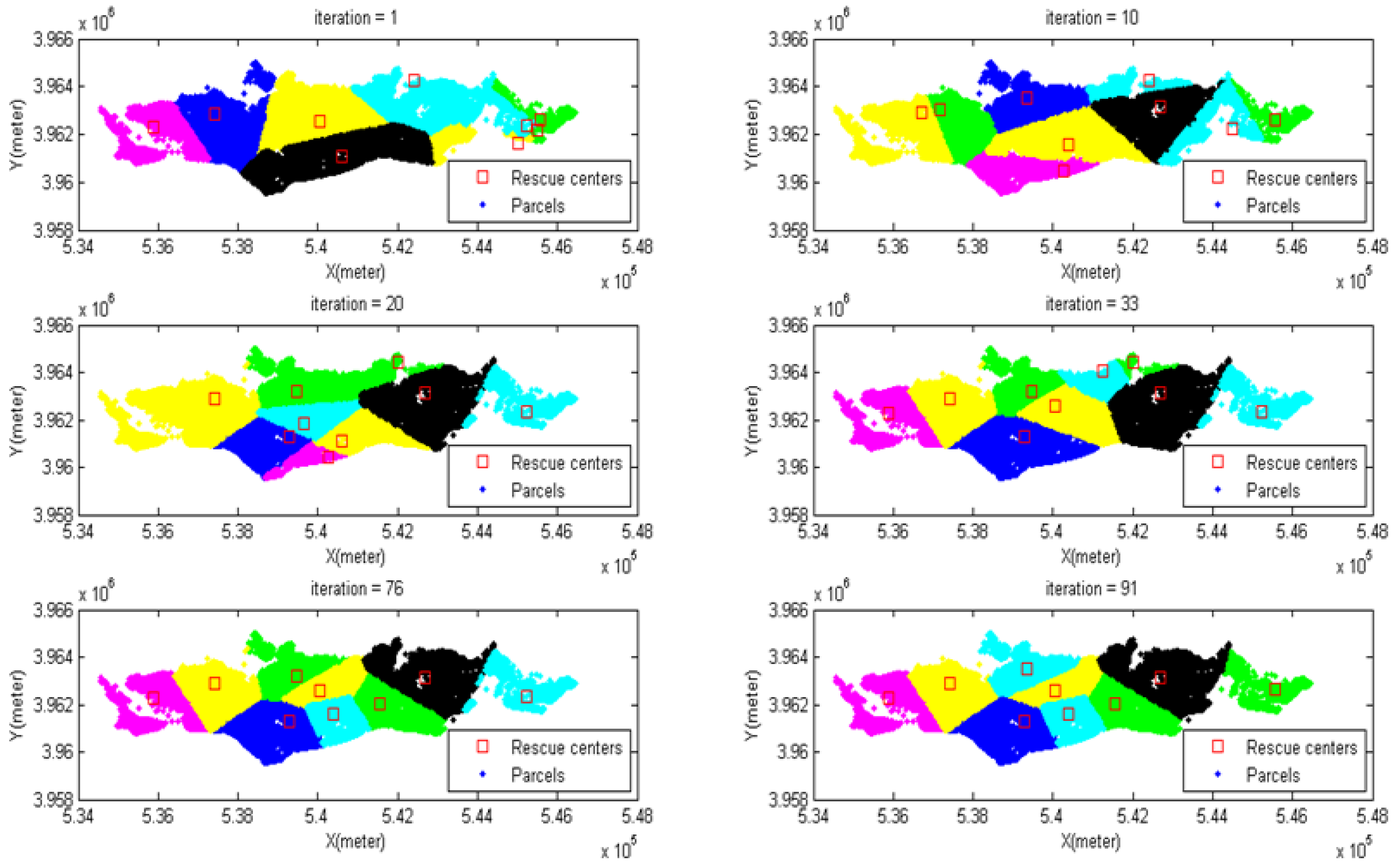
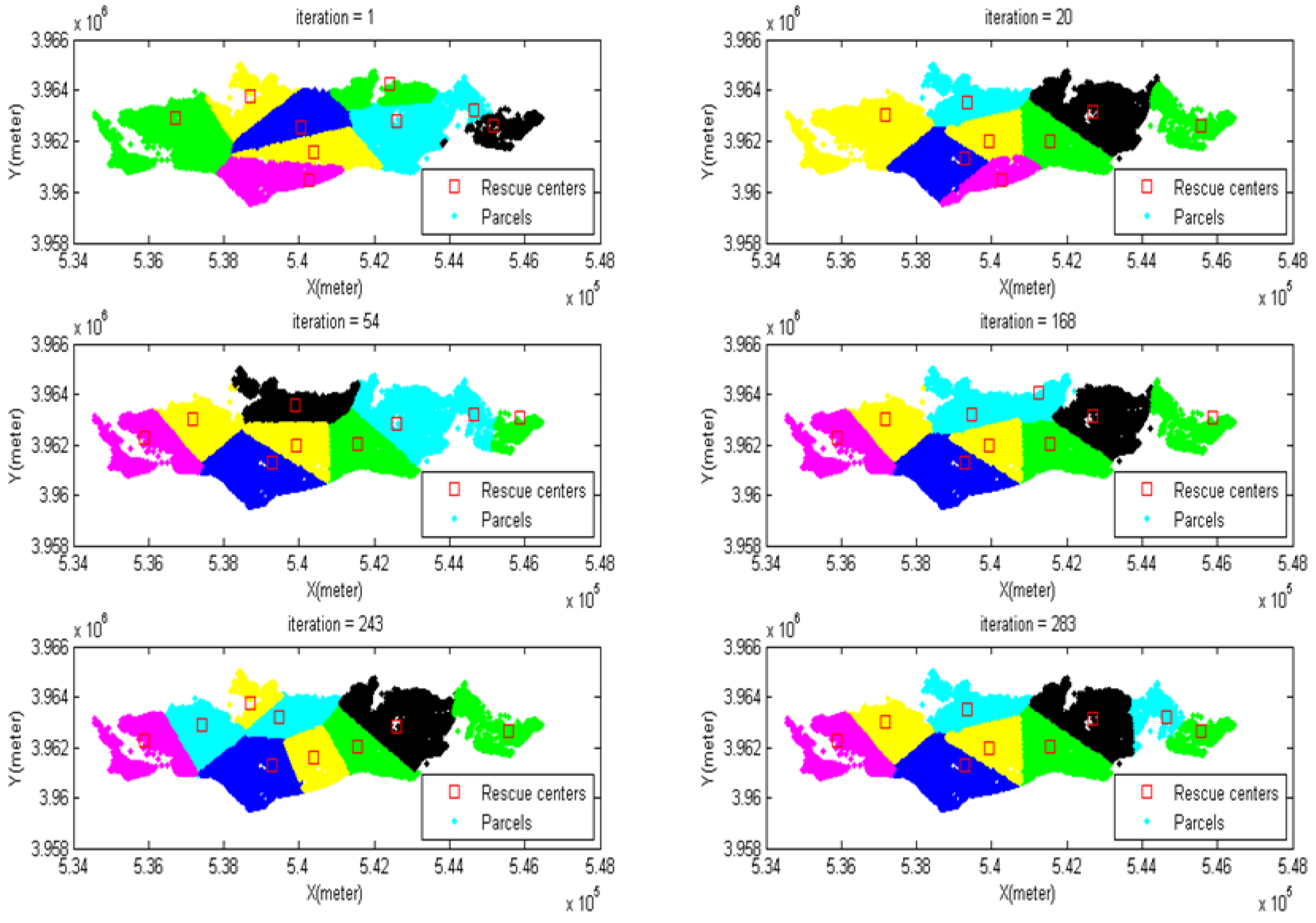
4.8. Modeling the Meta-Heuristic Algorithms

In this section, the way to model the allocation of parcel to the temporary relief centers is explained through PSO and ACO algorithms.

4.8.1. Modeling PSO

Since PSO is originally designed for continuous space, some methods are proposed to implement it for problems in discrete space. In this paper, the binary method proposed by Kennedy and Eberhart [77] is used. In the following, the main steps of implementing this method are described.

● Definition of the problem and fitness function

The purpose of optimization is to find the best combination of centers from the initially selected ones, to cover the district appropriately, with minimum distance from the parcels allocated to them. The fitness function is defined as the reverse of the total distances of parcels to their closest service center. In fact, the allocation of the parcels to the selected centers is carried out based on their distance from the centers. In other words, each parcel is mostly assigned to its closest selected center.

● Particle definition

In binary PSO, the components are 0 and 1 and the position of each particle is a binary vector. Since 9 centers out of 39 centers should be chosen, particle coding is defined as an array of 1 × 39, in which the members related to selected centers are 1 and the rest are zero. In Figure 9, coding of a particle is shown as an example.

It should be mentioned that having 9 as the number of sites is completely arbitrary. This number can be determined according to the availability of the facilities and personnel.

● Making the initial particles

The initial particles are made randomly. To build a particle, 9 digits between 1 and 39 are chosen randomly with no repetition. According to these selected digits, related elements of a 1 × 39 array are assigned as 1 and the rest are assigned as 0.

● Assessing the fitness function and determining the best previous position of particles

The fitness function should be calculated for each particle. The fitness function is considered as the reverse of total distances. If the fitness function of the current position is better than the PB, then it will replace the PB. In the first run, the current position of each particle is considered as its PB. It means that the particle movement is a combination of its previous movement and the movement towards GB.

● Definition of neighborhood to determine the global best

Two types of geographic and social neighborhoods can be defined in PSO. In this case, the social neighborhood is preferred. By definition, when producing the particles, they should be marked (in order of production). According to these ordering marks, some neighborhoods are defined. For example, each five successive particles are one neighborhood. Later, the global best for each particle is determined among its neighbors.

● Updating velocity and position vectors

The velocity for each particle is defined as an array of 1 × 39. Inside each member of this array, the velocity related to the corresponding member of the particle is placed. For example, for particle of Figure 9, the velocity vector is shown as Figure 10.

Now, assume that the particle of Figure 9 wants to move according to the velocity of Figure 10. To do so, a sigmoid function is used. Then, the velocity update means calculating the possibility of changing zero to one, or one to zero. The values of velocity, which are real numbers, should be transformed into probability values between zero and one. In fact, to calculate the possibility that the corresponding component in a particle array changes from zero to one, or vice versa, the sigmoid function (Equation (3)) is used [77].

$$sig(v)=\frac{1}{1+e^{-v}}\in [0,1],$$

(3)

In this equation, v is the velocity of each element from the 1 × 39 velocity array. In fact, the sigmoid function of Equation (3) is applied for every element of the array, and all the elements of this array are transferred to a new space (between zero and one) (Figure 11).

After applying the sigmoid function, the value of each component is defined using Equation (4) [77].

$$\begin{gathered} if\left(rand()<S(v_{id})\right)then x_{id}=1; \\ else x_{id}=0 \end{gathered}$$

(4)

In fact, for each element of every particle, a random number between zero and one is chosen. If this number is smaller than the corresponding sigmoid function (Figure 11), then the value one is given to this element; otherwise it will be zero. According to these values, the position of particles is updated. If the value of each component that was defined using Equation (4) equals 1, then the position of the component (Figure 9) is changed zero to one, or one to zero; otherwise, the position of the component is not changed.

After calculating the value for a particle, there should be nine 1 values and thirty 0 values. If the number of 1 values is less or more than nine, then enough 0 values should randomly be transferred into 1, or vice versa, respectively.

● Stop conditions

The stop condition could be defined as to achieve a predefined accuracy, a specified number of iteration, a time limit, or any combination of these. In this paper, achieving a specified number of iteration is considered as the stopping condition of the algorithm.

4.8.2. Modeling ACO

Different versions of ACO have already been developed. Their main difference comes from the way they update the pheromones. Considering the advantages reported by [78], the Ant System version is used in this study. In this algorithm, the descriptions of the problem, fitness function, fitness function assessment, and stop conditions are exactly the same as the previous algorithm.

● Construction of ant

In this research, a solution (ant) is a sequential selection of 9 centers out of the 39 candidate centers. To solve the optimization problem using the Ant System, solution space could be shown by a connected graph. The nodes are the 39 candidate centers, and there is an edge from every node to all others. First, a pre-specified amount of pheromone is placed on all graph nodes (candidate relief centers). As shown in Figure 12, the ants are constructed by stepwise moving from one node to another [6]. The possibility of moving from node i to node j for k-th ant is calculated by Equation (5) [78].

$$p_{ij}^k(t)=\{\begin{array}{cc}\hfill \frac{{[{\tau }_{ij}(t)]}^{\alpha }.{[{\eta }_{ij}]}^{\beta }}{{{\displaystyle \sum }}_{l\in allowe{d}_k}{[{\tau }_{il}(t)]}^{\alpha }.{[{\eta }_{il}]}^{\beta }},& if j\in allowe{d}_k\hfill \\ \hfill 0,& otherwise\hfill \end{array},$$

(5)

In this equation, allowed_k is the list of nodes that are not already covered by the k-th ant, τ_ij is the pheromone of the edge i-j (or the node j), α and β are controlling parameters and η is the heuristic function [78]. The next nodes are chosen based on the roulette wheel method using the probabilities calculated by Equation (5).

Normally, η is determined by a greedy rule (heuristic) [6]. In this problem, the heuristic function is defined by Equation (6). Here, d_ij is the minimum distance of the node from other nodes not-visited by the ant [78]. The node with smaller d_ij has a higher chance of being selected.

$${\eta }_{ij}=\frac{1}{d_{ij}},$$

(6)

● Pheromone update

After all ants constructed their paths, the pheromone is updated locally and is based on the value of the fitness function, using Equation 7 [6,78].

$${\tau }_{ij}\leftarrow (1-\rho ).{\tau }_{ij}+{{\displaystyle \sum }}_{k=1}^m\Delta {\tau }_{ij}^k,$$

(7)

where ρ is rate of evaporation, m is number of ants, $\Delta {\tau }_{ij}^k$ is the value of pheromone given to the edge i-j by the k-th ant. This value is calculated by Equation 8 [78].

$$\Delta {\tau }_{ij}^k=\{\begin{array}{cc}\hfill \frac{Q}{L_k},& if ant k used edge \left(i,j\right) in its tour\hfill \\ \hfill 0,& otherwise\hfill \end{array}$$

(8)

In this equation Q is a constant, L_k is the cost or the reverse of the fitness function for the k-th ant, which is the total distance of the parcels from their closest service center. For faster convergence of the algorithm, the pheromones are updated only by a small group of ants with the best fitness functions.

5. The Result of Algorithm Implementation

Following the objectives of the study, 39 sites were selected using TOPSIS and the proposed clustering method. Then, the PSO and ACO algorithms were used to select 9 final sites, with optimal allocation of parcels to them.

The values of the parameters for the two algorithms are defined by a regular trial and error process. In

Table 3. The optimized values for the parameter of PSO and ACO.

PSO		ACO
Parameter	Value	Parameter	Value
number of Particle	30	number of Ant	30
w	1	α	1
C1	2	β	0.5
C2	2	Q	10,000
initial velocity	0	evaporate rate (ρ)	0.1
min & max velocity	±4
Φ1 & Φ2	Rand (0,1)

, the optimal values found for those parameter are presented.

The PSO algorithm is executed 10 times and the best execution, regarding the objective function, is selected. Figure 13 shows the convergence of the PSO algorithm towards the optimum solution, in that best execution. In other words, it presents the best solutions found in different iterations of the execution. The minimum value for the total distance of parcels to centers was 27,107,098.169 m.

As is evident in Figure 13, the changes are insignificant from 76 to 91 iterations, and the algorithm converged in iteration number 91. Similarly, Figure 14 shows the convergence of the ACO algorithm in its best execution. Here, the minimum value for the total distance was found as 27,520,651.376 meters. In Figure 14, the changes are insignificant from 168 onwards, and the algorithm converged in implementation number 283.

As can be observed in Figure 13 and Figure 14, the last response related to two algorithms has a high correspondence.

5.1. Results Comparison

To compare the algorithms, the fitness function, convergence rate, constancy repeatability, and complexity of run time are used.

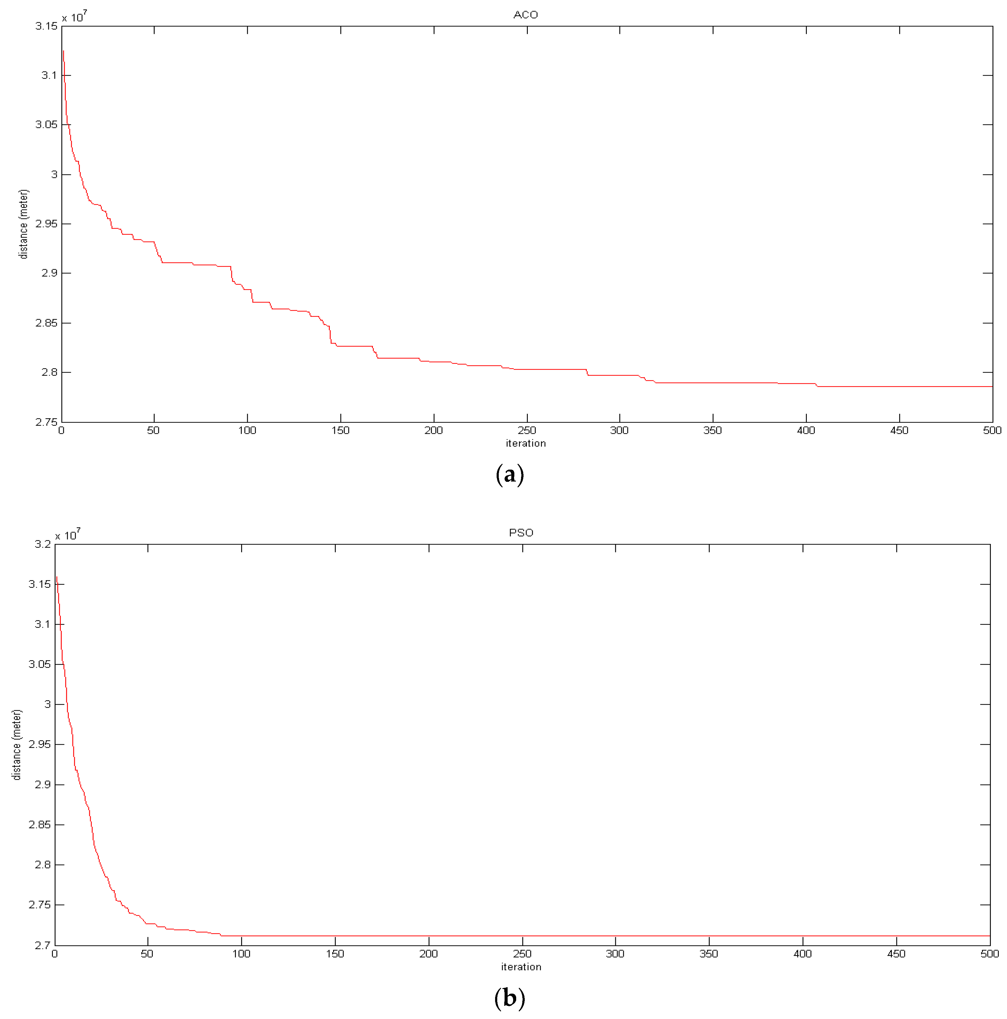
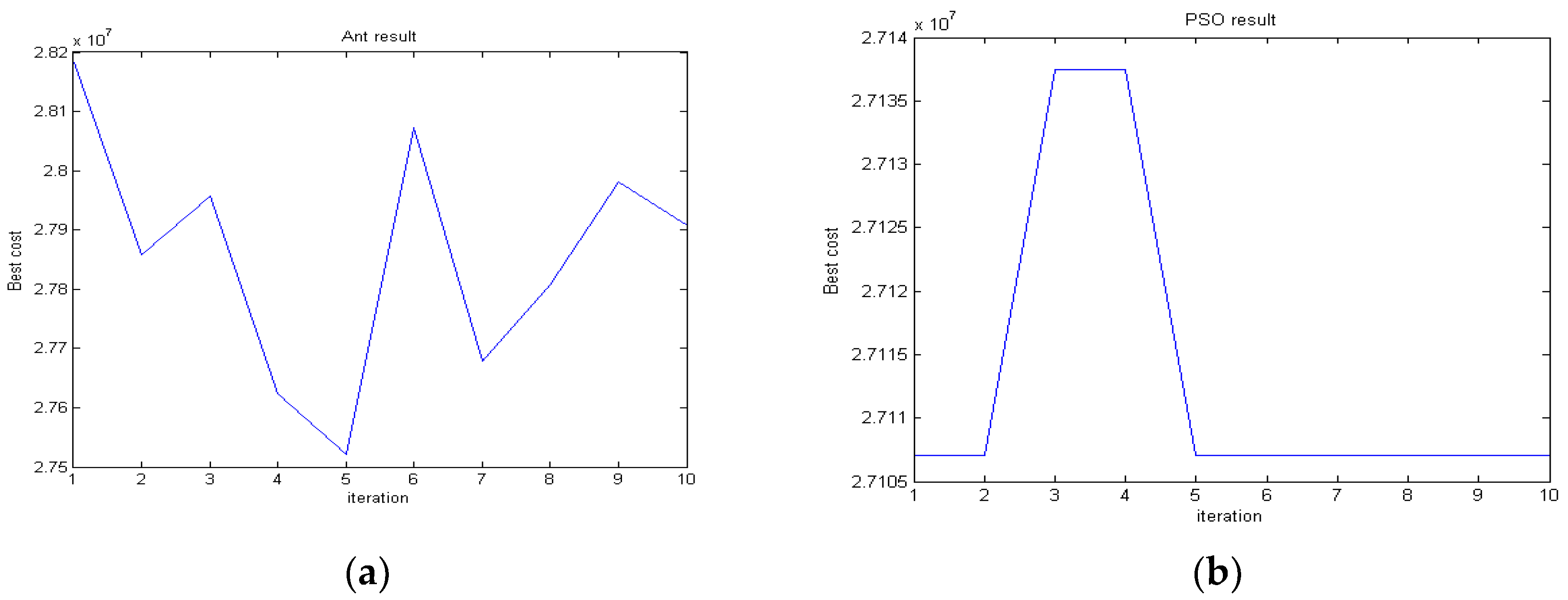
5.1.1. Comparing Fitness Function Values

Considering the implementation results of the algorithms, as shown in Figure 13 and Figure 14, the final responses under which PSO and ACO are converged are 27,107,098.169 and 27,520,651.376 meters, respectively. Thus, the PSO algorithm reached a better answer, with a smaller distance, i.e., 413 km, which means a 1.5 percent improvement.

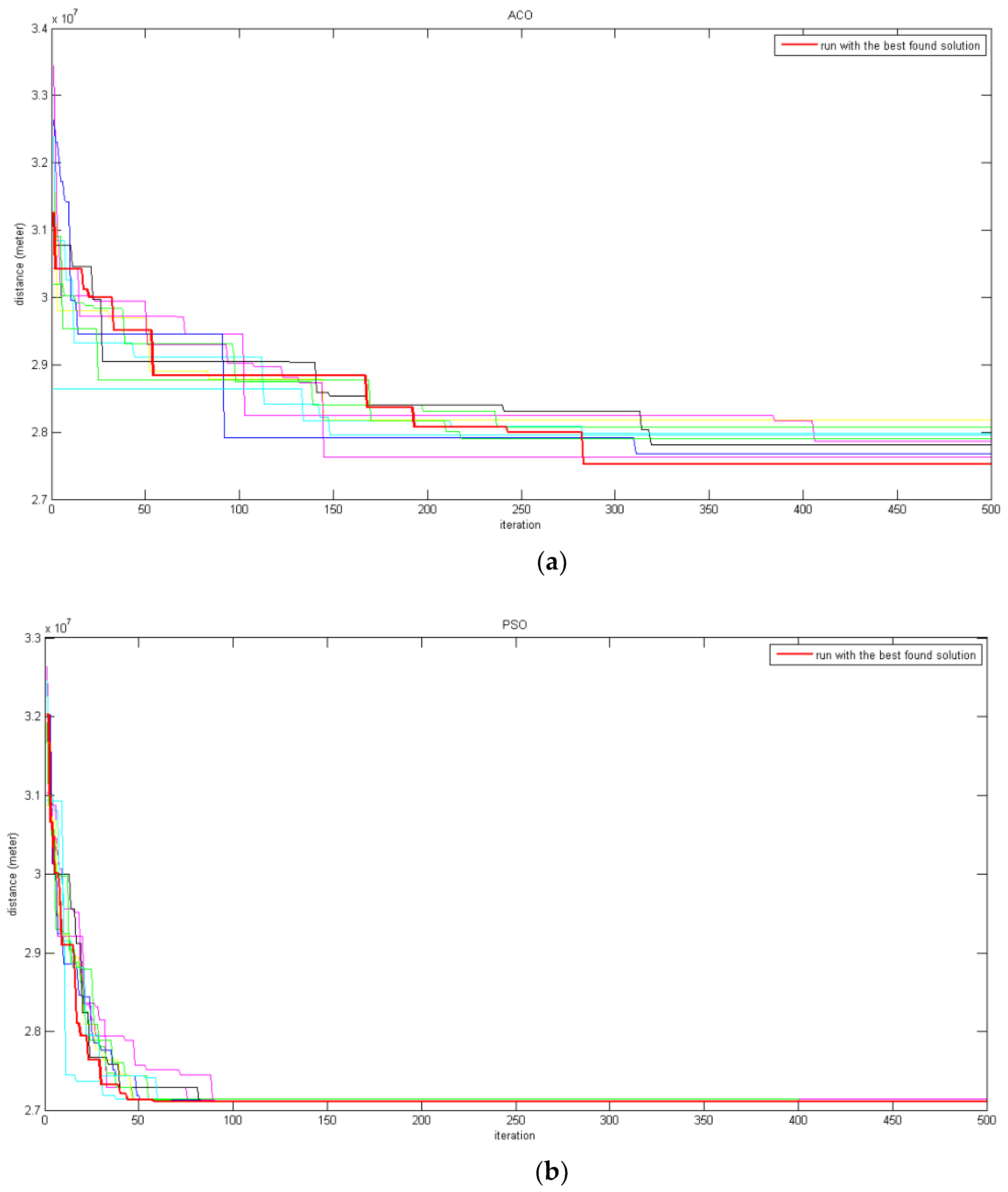
5.1.2. Comparing the Convergence Rate of the Algorithms

Figure 15 presents the convergence rate of the two algorithms for 10 different executions (runs). It shows that the convergence of both algorithms is satisfactory.

Considering the diagrams of Figure 15, the following can be observed:

• The convergence of the PSO is much smoother than that of ACO in all runs. This shows that, in this study, PSO is stronger than ACO in dealing with local optimums.
• The convergence rate is faster in the earlier iterations of both algorithms.
• In general, the convergence rate of PSO is higher (better) than that of ACO. In other words, in all executions including the best ones (presented by red color), PSO convergences to lower values of the objective function much faster than ACO. In addition, the best values found by PSO in iteration 90 are not found by ACO, even in iteration 500.
• In all iterations of the algorithms, the diagrams of PSO are more similar than those of ACO. In other words, the convergence rates of PSO for different executions are more similar than the convergence rates of ACO. Additionally, in the final iterations, any execution of ACO converges to a different value. This means that, apparently PSO is more robust and repeatable than ACO. To examine this further, a repeatability test is carried out and presented in the next section of the article.

In Figure 16, for each iteration, the average of the best values found by 10 different executions is presented.

Figure 16 shows again the smoother and faster convergence of the PSO compared with the ACO. The gradual change and smoothness of the PSO diagram reconfirms its higher repeatability and supremacy in dealing with local optimums. The stability of the PSO diagram, after iteration about 90, shows that many executions converged to the same value at iteration 90, without any fluctuation.

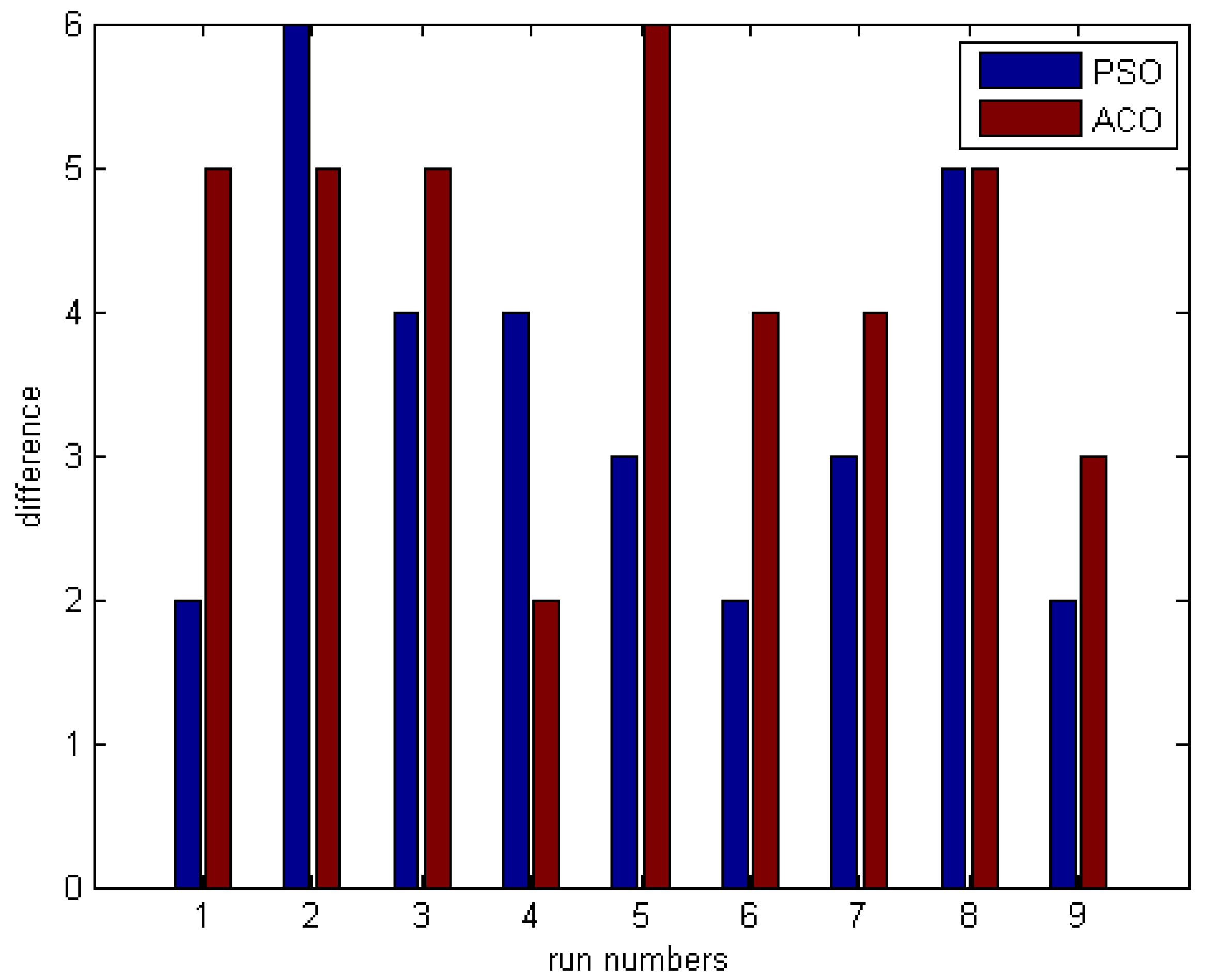
5.1.3. Comparing Algorithm Constancy

A good optimization algorithm is supposed to generate more similar results for different implementations with the same input values. This criterion is called algorithm repeatability. To investigate this parameter, each algorithm was implemented 10 times. Figure 17 shows the result for sequential repetitions of both algorithms.

The results of PSO can be divided into two different groups, with constant results in each group. In comparison, ACO generated more fluctuating results. The standard deviation of the results for PSO and ACO algorithms, as presented in Figure 17, are 12,817.050 and 206,670.896 respectively, which shows the higher (better) repeatability of the PSO.

The analyses and comparisons of the algorithms in the previous sections were related to the objective function. In the following, the final results, i.e., the 9 selected centers, are discussed. The best solutions in 10 executions of PSO and ACO are presented in Figure 13 (iteration 91) and Figure 14 (iteration 283), in that order. The two best solutions have 7 centers in common.

In the following, the results of 10 executions are discussed. The final result of each algorithm in each execution is 9 selected centers. The more these 9 centers are repeated in different executions of the algorithm, the more stable and repeatable the algorithm is. The best execution is selected as the base of comparison. For the other 9 executions, the altered centers, compared with the best execution, are counted. Figure 18 shows such differences, i.e., the count of altered centers.

As shown in Figure 18, the differences of the PSO executions from the PSO’s best execution are less than those of the ACO. The average of the differences for PSO and ACO are 3.4 and 4.3 respectively. This again reconfirms the superiority of PSO with regard to stability and repeatability.

5.1.4. Complexity of Run Time

The two algorithms are similar with regard to the fitness function calculation. Given the equal number of ants and particles, the count of fitness function calculations in each generation (iteration) in both algorithms is 30 (according to Table 3). However, the exact evaluation of the computational volume and complexity of the two algorithms is not an easy task. In this paper, only the run time of the algorithms was studied and compared. For this purpose, each algorithm is executed ten times, with the parameters defined in Table 3. The average time of these 10 runs is used as another criterion for comparing the two algorithms. The average run times of the PSO and ACO algorithms are 9464 and 10,671 s, respectively.

6. Conclusions

Selecting the correct positions for temporary relief centers can affect both the response time and efficiency of the relief activities after the earthquake. So far, different methods have been suggested for this issue. In this research, a very simple clustering method is proposed and used along with TOPSIS to initially select proper candidate centers on the basis of their land use, area, distance from the fault lines and main routes, slope and population. Therefore, the results of these two methods were not evaluated.

The goal was to select a limited number of centers (9 centers) among these sites such that the parcels could be optimally allocated to them. This makes the subject a complex optimization problem with a wide search space. Therefore, the two promising meta-heuristic algorithms of PSO and ACO were selected to be used. As mentioned in the previous work section, the considered location-allocation scenario is essentially a discrete problem, which can be solved by ACO. In contrast, PSO was originally developed for continuous search spaces. Therefore, a discrete version of PSO is used in this research. The results of the implementation confirmed the appropriateness of both algorithms. The PSO algorithm generated much better results. In comparison, the PSO algorithm converges faster. In addition, the results indicate a higher level of repeatability for PSO. In general, it could be concluded that in the location-allocation problem under consideration, the PSO algorithm showed better performance than the ACO algorithm.

Many uncovered aspects of this research can be considered for future work. First, considering the importance of accessibility distance to the post-earthquake relief centers, it is better to minimize the farthest distance for allocation (the farthest distance a parcel has from the center it is assigned to, among all other parcels). Secondly, in this research, six parameters were considered in TOPSIS model for initial selection of the centers. However, it would be more reasonable to incorporate them directly in the optimization. As was mentioned in Section 4.4, including these parameters in optimization makes the modeling too complex due to their number and the difference in the parameters. A solution can be to enter them into the TOPSIS model. Then, the output of TOPSIS, which are the CL values, could also be entered into optimization and be incorporated with the distance-based objective function. It means that the sum of the CL values for all final selected centers should be maximized. Obviously, testing of the capabilities of other meta-heuristic algorithms to solve the problem could also be interesting. As already mentioned, in this study, the point allocation method and the opinions of a single expert are used for defining the criteria-weights in TOPSIS analyses. In the continuation of the research, other methods of criteria weighting, the integration of different experts’ opinion, and group decision making methods can be considered. One of the problems when using TOPSIS is its compensation aspect. It means that a choice with a bad parameter can be selected because that choice is very good regarding other parameters. For example, in this research, the center ‘7’ was among the finally selected ones, since it is appropriate regarding most parameters. However, this center is inappropriate because of its small area (86.200 square meters). This problem could be partly controlled by a pre-process before going to the TOPSIS model. For example, the sites could be removed, where they are in one or more parameters lower than a limit. Another important shortcoming of this research is the allocation of parcels to the centers without considering the center’s capacity. Therefore, the population allocated to a center can be very different from its capacity. To solve this, the difference between each center capacity and parcels allocated to it can be considered as a constraint or even an optimization objective.

References

1. Hualou, L. Disaster prevention and management: A Geographical Perspective. Dis. Adv. 2011, 4, 3–5. [Google Scholar]
2. Saeedy, S.; Shamsipour, A.A.; Fallah, S.; Saeedy, S. Evaluation of Relief and Rescue Operations in Historic Regions (Case of Study: Fahadan District in Yazd City, Iran). Available online: https://www.researchgate.net/profile/Aliakbar_Shamsipour/publication/260136058_Evaluation_of_Relief_and_Rescue_Operations_in_Historic_Regions_Case_of_Study_Fahadan_District_in_Yazd_City_Iran/links/00b4952fb804d64012000000/Evaluation-of-Relief-and-Rescue-Operations-in-Historic-Regions-Case-of-Study-Fahadan-District-in-Yazd-City-Iran.pdf (accessed on 30 May 2018).
3. Soltani, A.; Ardalan, A.; Boloorani, A.D.; Haghdoost, A.; Hosseinzadeh-Attar, M.J. Site selection criteria for sheltering after earthquakes: A systematic review. PLoS Curr. 2014. [Google Scholar] [CrossRef] [PubMed]
4. Bramante, J.F.; Raju, D.K. Predicting the distribution of informal camps established by the displaced after a catastrophic disaster, Port-au-Prince, Haiti. Appl. Geogr. 2013, 40, 30–39. [Google Scholar] [CrossRef]
5. Aras, N.; Orbay, M.; Altinel, I. Efficient heuristics for the rectilinear distance capacitated multi-facility Weber problem. J. Oper. Res. Soc. 2008, 59, 64–79. [Google Scholar] [CrossRef]
6. Arnaout, J.-P. Ant colony optimization algorithm for the Euclidean location-allocation problem with unknown number of facilities. J. Intell. Manuf. 2013, 24, 45–54. [Google Scholar] [CrossRef]
7. Ghosh, A.; Rushton, G. Spatial Analysis and Location-Allocation Models; Van Nostrand Reinhold Company: New York, NY, USA, 1987. [Google Scholar]
8. Saeidian, B.; Mesgari, M.S.; Ghodousi, M. Evaluation and comparison of genetic algorithm and bees algorithm for location–allocation of earthquake relief centers. Int. J. Dis. Risk Reduct. 2016, 15, 94–107. [Google Scholar] [CrossRef]
9. Beraldi, P.; Bruni, M.E. A probabilistic model applied to emergency service vehicle location. Eur. J. Oper. Res. 2009, 196, 323–331. [Google Scholar] [CrossRef]
10. Tzeng, G.-H.; Cheng, H.-J.; Huang, T.D. Multi-objective optimal planning for designing relief delivery systems. Transp. Res. Part E 2007, 43, 673–686. [Google Scholar] [CrossRef]
11. Balcik, B.; Beamon, B.M. Facility location in humanitarian relief. Int. J. Logist. 2008, 11, 101–121. [Google Scholar] [CrossRef]
12. Hooshangi, N.; Alesheikh, A.A. Agent-based task allocation under uncertainties in disaster environments: An approach to interval uncertainty. Int. J. Dis. Risk Reduct. 2017, 24, 160–171. [Google Scholar] [CrossRef]
13. Mingang, Z.; Zeng, M.; Xiaoyan, W. Research on location-routing problem of relief system based on emergency logistics. In Proceedings of the 16th International Conference on Industrial Engineering and Engineering Management, Beijing, China, 21–23 October 2009. [Google Scholar]
14. Memon, I.; Mangi, F.A.; Jamro, D.A. Collision avoidance of intelligent service robot for industrial security system. IJCSI Int. J. Comput. Sci. Issues 2013, 10, 397–401. [Google Scholar]
15. Saeidian, B.; Mesgari, M.S.; Ghodousi, M. Optimum allocation of water to the cultivation farms using Genetic Algorithm. Int. Arch. Photogramm. Remote Sens. Spat. Inf. Sci. 2015, 40, 631–638. [Google Scholar] [CrossRef]
16. Yi, W.; Kumar, A. Ant colony optimization for disaster relief operations. Transp. Res. Part E 2007, 43, 660–672. [Google Scholar] [CrossRef]
17. Sheu, J.-B. An emergency logistics distribution approach for quick response to urgent relief demand in disasters. Transp. Res. Part E 2007, 43, 687–709. [Google Scholar] [CrossRef]
18. Ohlemüller, M. Tabu search for large location-allocation problems. J. Oper. Res. Soc. 1997, 48, 745–750. [Google Scholar] [CrossRef]
19. Brimberg, J.; Hansen, P.; Mladenović, N.; Taillard, E.D. Improvements and comparison of heuristics for solving the uncapacitated multisource Weber problem. Oper. Res. 2000, 48, 444–460. [Google Scholar] [CrossRef]
20. Zheng, Y.-J.; Chen, S.-Y.; Ling, H.-F. Evolutionary optimization for disaster relief operations: A survey. Appl. Soft Comput. 2015, 27, 553–566. [Google Scholar] [CrossRef]
21. Li, X.; Zhao, Z.; Zhu, X.; Wyatt, T. Covering models and optimization techniques for emergency response facility location and planning: A review. Math. Methods Oper. Res. 2011, 74, 281–310. [Google Scholar] [CrossRef]
22. Mirjalili, S. Dragonfly algorithm: A new meta-heuristic optimization technique for solving single-objective, discrete, and multi-objective problems. Neural Comput. Appl. 2016, 27, 1053–1073. [Google Scholar] [CrossRef]
23. Askarzadeh, A. A novel metaheuristic method for solving constrained engineering optimization problems: Crow search algorithm. Comput. Struct. 2016, 169, 1–12. [Google Scholar] [CrossRef]
24. Mirjalili, S.; Lewis, A. The whale optimization algorithm. Adv. Eng. Softw. 2016, 95, 51–67. [Google Scholar] [CrossRef]
25. Salimi, H. Stochastic fractal search: A powerful metaheuristic algorithm. Knowl. Based Syst. 2015, 75, 1–18. [Google Scholar] [CrossRef]
26. Shbib, R.; Zhou, S.; Al-Mosawi, M. Optimal route selection method with ant colony optimization (ACO) for Cognitive network in disaster information network. Available online: https://www.researchgate.net/publication/229088815_Optimal_Route_Selection_Method_with_Ant_Colony_Optimization_ACO_for_Cognitive_Network_in_Disaster_Information_Network (accessed on 30 May 2018).
27. Tian, J.; Ma, W.-Z.; Wang, Y.-L.; Wang, K.-L. Emergency supplies distributing and vehicle routes programming based on particle swarm optimization. Syst. Eng. Theory Pract. 2011, 5, 898–906. [Google Scholar]
28. Yunxiao, Q.L.J.H.L.; Jiayi, H. Mix K-Means Clustering with Ant Colony Optimization Used in City Emergency Rescue Decision-Making; China Public Security: Beijing, China, 2011.
29. Zade, A.-V.; Tugnayat, R.-M. Ant Colony Optimization (ACO) in disaster information network. Int. J. Innov. Eng. Res. Technol. 2014, 1, 1–5. [Google Scholar]
30. Zheng, Y.-J.; Ling, H.-F.; Xue, J.-Y.; Chen, S.-Y. Population classification in fire evacuation: A multiobjective particle swarm optimization approach. IEEE Trans. Evol. Comput. 2014, 18, 70–81. [Google Scholar] [CrossRef]
31. Hu, F.; Xu, W.; Li, X. A modified particle swarm optimization algorithm for optimal allocation of earthquake emergency shelters. Int. J. Geogr. Inf. Sci. 2012, 26, 1643–1666. [Google Scholar] [CrossRef]
32. Chaharsooghi, S.K.; Kermani, A.H.M. An effective ant colony optimization algorithm (ACO) for multi-objective resource allocation problem (MORAP). Appl. Math. Comput. 2008, 200, 167–177. [Google Scholar] [CrossRef]
33. Garg, H.; Sharma, S. Multi-objective reliability-redundancy allocation problem using particle swarm optimization. Comput. Ind. Eng. 2013, 64, 247–255. [Google Scholar] [CrossRef]
34. Gong, Y.-J.; Zhang, J.; Chung, H.S.-H.; Chen, W.-N.; Zhan, Z.-H.; Li, Y.; Shi, Y.-H. An efficient resource allocation scheme using particle swarm optimization. IEEE Trans. Evol. Comput. 2012, 16, 801–816. [Google Scholar] [CrossRef]
35. Liang, Y.-C.; Smith, A.E. An ant colony optimization algorithm for the redundancy allocation problem (RAP). IEEE Trans. Reliab. 2004, 53, 417–423. [Google Scholar] [CrossRef]
36. Saravanan, M.; Slochanal, S.M.R.; Venkatesh, P.; Abraham, P.S. Application of PSO technique for optimal location of FACTS devices considering system loadability and cost of installation. In Proceedings of the International Power Engineering Conference, Singapore, 29 November–2 December 2005. [Google Scholar]
37. Vilovic, I.; Burum, N.; Sipus, Z. Ant colony approach in optimization of base station position. In Proceedings of the 3rd European Conference on Antennas and Propagation, Berlin, Germany, 23–27 March 2009. [Google Scholar]
38. Wang, K.-J.; Lee, C.-H. A revised ant algorithm for solving location–allocation problem with risky demand in a multi-echelon supply chain network. Appl. Soft Comput. 2015, 32, 311–321. [Google Scholar] [CrossRef]
39. Yin, P.-Y.; Wang, J.-Y. Ant colony optimization for the nonlinear resource allocation problem. Appl. Math. Comput. 2006, 174, 1438–1453. [Google Scholar] [CrossRef]
40. Yin, P.-Y.; Wang, J.-Y. A particle swarm optimization approach to the nonlinear resource allocation problem. Appl. Math. Comput. 2006, 183, 232–242. [Google Scholar] [CrossRef]
41. Aghababa, M.P.; Amrollahi, M.H.; Borjkhani, M. Application of GA, PSO, and ACO algorithms to path planning of autonomous underwater vehicles. J. Marine Sci. Appl. 2012, 11, 378–386. [Google Scholar] [CrossRef]
42. Elbeltagi, E.; Hegazy, T.; Grierson, D. Comparison among five evolutionary-based optimization algorithms. Adv. Eng. Inf. 2005, 19, 43–53. [Google Scholar] [CrossRef]
43. Hasan, M.K.; Ismail, A.F.; Islam, S.; Hashim, W.; Ahmed, M.M.; Memon, I. A novel HGBBDSA-CTI approach for subcarrier allocation in heterogeneous network. Telecommun. Syst. 2018. [Google Scholar] [CrossRef]
44. Marinakis, Y.; Marinaki, M.; Doumpos, M.; Zopounidis, C. Ant colony and particle swarm optimization for financial classification problems. Expert Syst. Appl. 2009, 36, 10604–10611. [Google Scholar] [CrossRef]
45. Moussouni, F.; Brisset, S.; Brochet, P. Comparison of two multi-agent algorithms: ACO and PSO for the optimization of a brushless DC wheel motor. In Intelligent Computer Techniques in Applied Electromagnetics; Springer: Berlin, Germany, 2008. [Google Scholar]
46. Selvi, V.; Umarani, D.R. Comparative analysis of ant colony and particle swarm optimization techniques. Int. J. Comput. Appl. 2010, 5. [Google Scholar] [CrossRef]
47. Shakerian, R.; Kamali, S.H.; Hedayati, M.; Alipour, M. Comparative study of ant colony optimization and particle swarm optimization for grid scheduling. J. Math. Comput. Sci. 2011, 2, 469–474. [Google Scholar]
48. Vilovic, I.; Burum, N.; Sipus, Z.; Nad, R. PSO and ACO algorithms applied to location optimization of the WLAN base station. In Proceedings of the 19th International Conference on Applied Electromagnetics and Communications, Dubrovnik, Croatia, 24–26 September 2007. [Google Scholar]
49. Adrian, A.M.; Utamima, A.; Wang, K.-J. A comparative study of GA, PSO and ACO for solving construction site layout optimization. KSCE J. Civ. Eng. 2015, 19, 520–527. [Google Scholar] [CrossRef]
50. Bailey, A.; Ornbuki-Berrnan, B.; Asobiela, S. Discrete pso for the uncapacitated single allocation hub location problem. In Proceedings of the IEEE Symposium on Computational Intelligence in Production and Logistics Systems (CIPLS), Singapore, 16–19 April 2013. [Google Scholar]
51. Guner, A.R.; Sevkli, M. A discrete particle swarm optimization algorithm for uncapacitated facility location problem. J. Artif. Evol. Appl. 2008, 10. [Google Scholar] [CrossRef]
52. Noory, H.; Liaghat, A.; Parsinejad, M.; Bozorg-Haddad, O. Optimizing irrigation water allocation and multicrop planning using discrete PSO algorithm. J. Irrig. Drain. Eng. 2011, 138, 437–444. [Google Scholar] [CrossRef]
53. Yu, X. Facility allocation based on hybrid discrete PSO under emergency. Inf. Technol. J. 2013, 12. [Google Scholar] [CrossRef]
54. Wolpert, D.H.; Macready, W.G. No free lunch theorems for optimization. IEEE Trans. Evol. Comput. 1997, 1, 67–82. [Google Scholar] [CrossRef] [Green Version]
55. Beni, G.; Wang, J. Swarm Intelligence in Cellular Robotic Systems, in Robots and Biological Systems: Towards a New Bionics? Springer: Berlin, Germany, 1993. [Google Scholar]
56. Dorigo, M. Optimization, Learning and Natural Algorithms; Politecnico di Milano: Milan, Italy, 1992. [Google Scholar]
57. Eberhart, R.C.; Kennedy, J. A new optimizer using particle swarm theory. In Proceedings of the 6th International Symposium on Micro Machine and Human Science, Nagoya, Japan, 4–6 October 1995. [Google Scholar]
58. Kennedy, J.; Eberhart, R.C. Particle swarm optimization. In Proceedings of the ICNN’95—International Conference on Neural Networks, Perth, WA, Australia, 27 November–1 December 1995. [Google Scholar]
59. Pham, D.T.; Ghanbarzadeh, A.; Koc, E.; Otri, S.; Rahim, S.; Zaidi, M. The Bees Algorithm; Manufacturing Engineering Centre, Cardiff University: Cardiff, UK, 2005. [Google Scholar]
60. Engelbrecht, A.P. Fundamentals of Computational Swarm Intelligence; Wile: Chichester, UK, 2005. [Google Scholar]
61. Heppner, F.; Grenander, U. A stochastic nonlinear model for coordinated bird flocks. Available online: https://www.researchgate.net/profile/Frank_Heppner/publication/278411001_A_Stochastic_Non-Linear_Model_for_Bird_Flocking/links/5580a02908aea3d7096e4c8a.pdf (accessed on 30 May 2018).
62. Poli, R.; Kennedy, J.; Blackwell, T. Particle swarm optimization. Swarm Intell. 2007, 1, 33–57. [Google Scholar] [CrossRef]
63. Samsami, R. Comparison between Genetic Algorithm (GA), Particle Swarm Optimization (PSO) and Ant Colony Optimization (ACO) Techniques for NO Emission Forecasting in Iran. World Appl. Sci. J. 2013, 28, 1996–2002. [Google Scholar]
64. Eberhart, R.C.; Shi, Y. Comparing inertia weights and constriction factors in particle swarm optimization. In Proceedings of the Congress on Evolutionary Computation. CEC00 (Cat. No.00TH8512), La Jolla, CA, USA, 16–19 July 2000. [Google Scholar]
65. Eberhart, R.C.; Shi, Y. Tracking and optimizing dynamic systems with particle swarms. In Proceedings of the Congress on Evolutionary Computation (IEEE Cat. No.01TH8546), Seoul, Korea, 27–30 May 2001. [Google Scholar]
66. Dorigo, M.; Blum, C. Ant colony optimization theory: A survey. Theor. Comput. Sci. 2005, 344, 243–278. [Google Scholar] [CrossRef]
67. Dorigo, M.; Gambardella, L.M. Ant colonies for the travelling salesman problem. BioSystems 1997, 43, 73–81. [Google Scholar] [CrossRef] [Green Version]
68. Dorigo, M.; Socha, K. An introduction to ant colony optimization. In Handbook of Approximation Algorithms and Metaheuristics; IRIDIA (Institut de Recherches Interdisciplinaires et de Developpements en Intelligence Artificielle): Bruxelles, Belgium, 2006. [Google Scholar]
69. Opricovic, S.; Tzeng, G.-H. Compromise solution by MCDM methods: A comparative analysis of VIKOR and TOPSIS. Eur. J. Oper. Res. 2004, 156, 445–455. [Google Scholar] [CrossRef]
70. Sarvar, H.; Amini, J.; Laleh-Poor, M. Assessment of risk caused by earthquake in region 1 of Tehran using the combination of RADIUS, TOPSIS and AHP models. J. Civ. Eng. Urban 2011, 1, 39–48. [Google Scholar]
71. Wikipedia. District 1 of Tehran municipality. 2017. Available online: https://fa.wikipedia.org/wiki/%D9%85%D9%86%D8%B7%D9%82%D9%87_%DB%B1_%D8%B4%D9%87%D8%B1%D8%AF%D8%A7%D8%B1%DB%8C_%D8%AA%D9%87%D8%B1%D8%A7%D9%86 (accessed on 30 May 2018).
72. Arain, Q.A.; Aslam Uqaili, M.; Deng, Z.; Memon, I.; Jiao, J.; Shaikh, M.A.; Zubedi, A.; Ashraf, A.; Arain, U.A. Clustering based energy efficient and communication protocol for multiple mix-zones over road networks. Wirel. Pers. Commun. 2017, 95, 411–428. [Google Scholar] [CrossRef]
73. Gustav, Y.H.; et al. Velocity similarity anonymization for continuous query location based services. In Proceedings of the International Conference on Computational Problem-Solving (ICCP), Jiuzhai, China, 26–28 October 2013. [Google Scholar]
74. Malczewski, J. GIS and Multicriteria Decision Analysis; John Wiley & Sons: Hoboken, NJ, USA, 1999. [Google Scholar]
75. Zardari, N.H.; Ahmed, K.; Shirazi, S.M.; Yusop, Z.B. Literature Review, in Weighting Methods and Their Effects on Multi-Criteria Decision Making Model Outcomes in Water Resources Management; Springer: Berlin, Germany, 2015. [Google Scholar]
76. Chen, Y.; Yu, J.; Khan, S. Spatial sensitivity analysis of multi-criteria weights in GIS-based land suitability evaluation. Environ. Model. Softw. 2010, 25, 1582–1591. [Google Scholar] [CrossRef]
77. Kennedy, J.; Eberhart, R.C. A discrete binary version of the particle swarm algorithm. In Proceedings of the IEEE International Conference on Systems, Man, and Cybernetics. Computational Cybernetics and Simulation, Orlando, FL, USA, 12–15 October 1997. [Google Scholar]
78. Dorigo, M.; Maniezzo, V.; Colorni, A. Ant system: Optimization by a colony of cooperating agents. IEEE Trans. Syst. Man Cybern. Part B 1996, 26, 29–41. [Google Scholar] [CrossRef] [PubMed]
Figure 1. The main stages of the study.
Ijgi 07 00292 g001
Figure 2. (a) Location of Tehran province in Iran (extracted from Google earth); (b) The position of district 1 of Tehran municipality (adapted from [71]).
Ijgi 07 00292 g002
Figure 3. The distance buffers from two fault lines close to district 1.
Ijgi 07 00292 g003
Figure 4. The distance buffers from the main routes of district 1.
Ijgi 07 00292 g004
Figure 5. Position of 150 sites with higher priority amongst other sites.
Ijgi 07 00292 g005
Figure 6. The result of sensitivity analyses: the count of altered sites (difference) caused by percentage of changes (pc) in the criterion-weight.
Ijgi 07 00292 g006
Figure 7. (a) The clustering carried out with a 250-meter threshold; (b) The final centers were achieved.
Ijgi 07 00292 g007
Figure 8. The counts and distribution of cluster centers resulting from different thresholds. (a) 50 meters; (b) 100 meters; (c) 150 meters; (d) 200 meters; (e) 300 meters; (f) 350 meters; (g) 400 meters; (h) 450 meters.
Ijgi 07 00292 g008aIjgi 07 00292 g008b
Figure 9. Coding a particle in a 1× 39 vector including zero and one.
Ijgi 07 00292 g009
Figure 10. Velocity of a particle.
Ijgi 07 00292 g010
Figure 11. The sigmoid of velocity for the velocity of Figure 10.
Ijgi 07 00292 g011
Figure 12. Shows movement of ants and making of an ant.
Ijgi 07 00292 g012
Figure 13. The result of the location-allocation using PSO with different iterations.
Ijgi 07 00292 g013
Figure 14. The result of the location-allocation using ACO with different iterations.
Ijgi 07 00292 g014
Figure 15. The convergence process of two algorithms for 10 different runs: (a) ACO; (b) PSO.
Ijgi 07 00292 g015
Figure 16. The average of the best values found by 10 executions, for different iterations: (a) for the ACO algorithm; (b) for the PSO algorithm.
Ijgi 07 00292 g016
Figure 17. Algorithm constancy in sequential repetitions: (a) ACO; (b) PSO.
Ijgi 07 00292 g017
Figure 18. The count of altered centers (difference) in the other 9 executions, compared with the best execution.
Ijgi 07 00292 g018