Figure 1.
Estimated coefficients for the pixels in the Airborne Visible/Infrared Imaging Spectrometer (AVIRIS) Indian Pines dataset (about 5% training pixels are used, see
Section 4), the corresponding class labels are included in the parentheses, and all coefficients are ranked in order of the class labels. (
a–
c): Pixel taken from Class C9, and the coefficients of C9 are in the range (219, 221]. (
d–
f): Pixel taken from Class C5, and the coefficients of C5 are in the range (129, 154]. (
g–
i): Pixel taken from Class C11, and the coefficients of C11 are in the range (270, 394]. (
a) KNLS (C9). (
b) KFCLS (C9). (
c) KSRC (C9). (
d) KNLS (C5). (
e) KFCLS (C5). (
f) KSRC (C5). (
g) KNLS (C11). (
h) KFCLS (C11). (
i) KSRC (C11). Notably, alternating direction method of multipliers (ADMM) is used to solve the optimization problems of KNLS and KFLCS, and thus their coefficients are not strictly nonnegative.
Figure 2.
Sum of the estimated coefficients for the pixels in the Airborne Visible/Infrared Imaging Spectrometer (AVIRIS) Indian Pines dataset (about 5% training pixels are used, see
Section 4), the corresponding class labels are included in the parentheses. (
a–
c): Pixel taken from Class C9. (
d–
f): Pixel taken from Class C5. (
g–
i): Pixel taken from Class C11. (
a) KNLS (C9). (
b) KFCLS (C9). (
c) KSRC (C9). (
d) KNLS (C5). (
e) KFCLS (C5). (
f) KSRC (C5). (
g) KNLS (C11). (
h) KFCLS (C11). (
i) KSRC (C11).
Figure 3.
AVIRIS Indian Pines dataset. (a) RGB composite image. (b) Ground reference map.
Figure 3.
AVIRIS Indian Pines dataset. (a) RGB composite image. (b) Ground reference map.
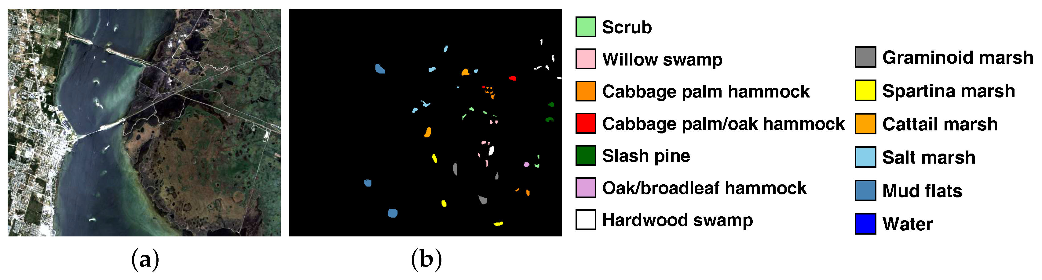
Figure 4.
AVIRIS Kennedy Space Center dataset. (a) RGB composite image. (b) Ground reference map.
Figure 4.
AVIRIS Kennedy Space Center dataset. (a) RGB composite image. (b) Ground reference map.
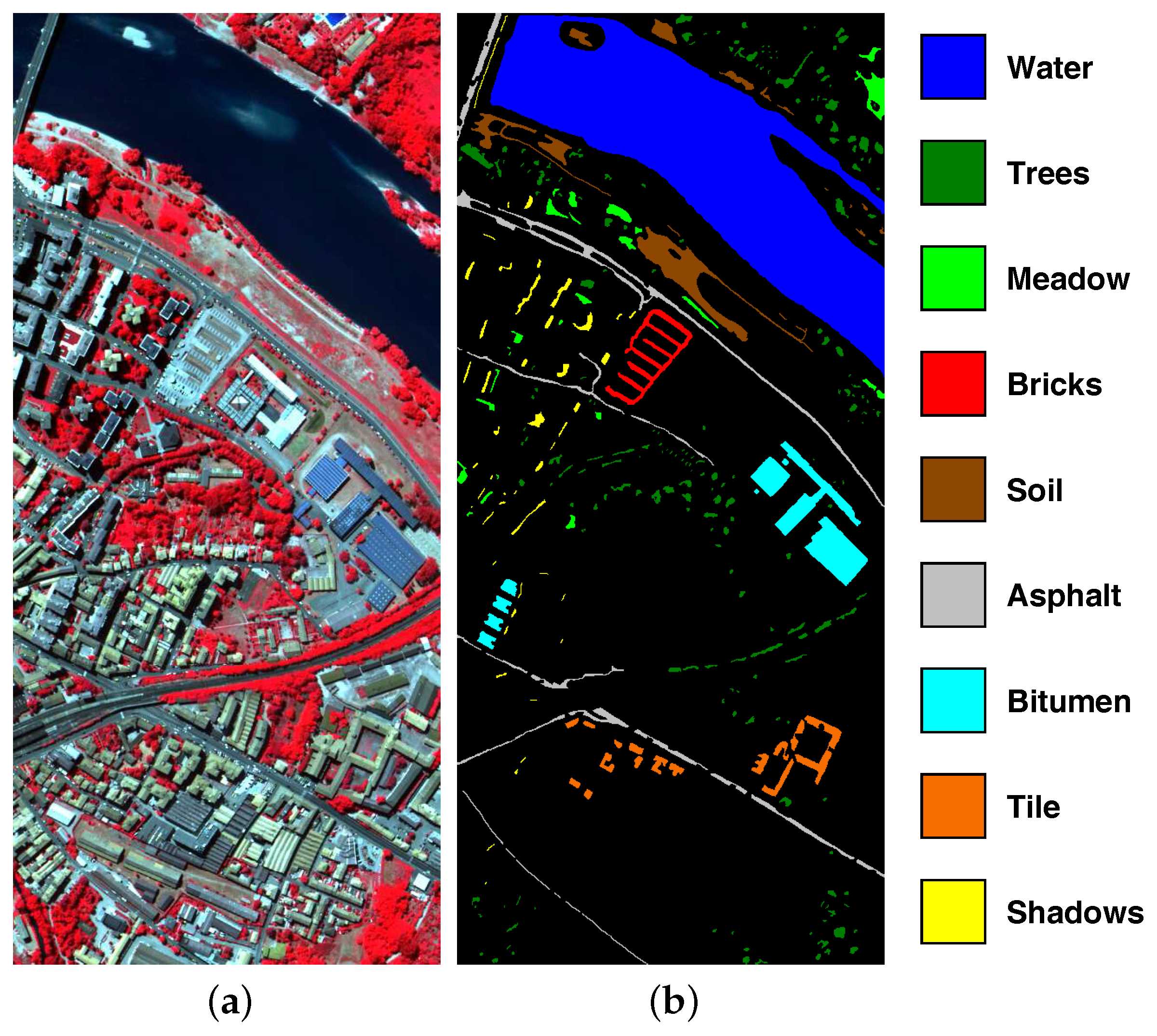
Figure 5.
Reflective Optics System Imaging Spectrometer (ROSIS) University of Pavia dataset. (a) RGB composite image. (b) Ground reference map.
Figure 5.
Reflective Optics System Imaging Spectrometer (ROSIS) University of Pavia dataset. (a) RGB composite image. (b) Ground reference map.
Figure 6.
ROSIS Center of Pavia dataset. (a) RGB composite image. (b) Ground reference map.
Figure 6.
ROSIS Center of Pavia dataset. (a) RGB composite image. (b) Ground reference map.
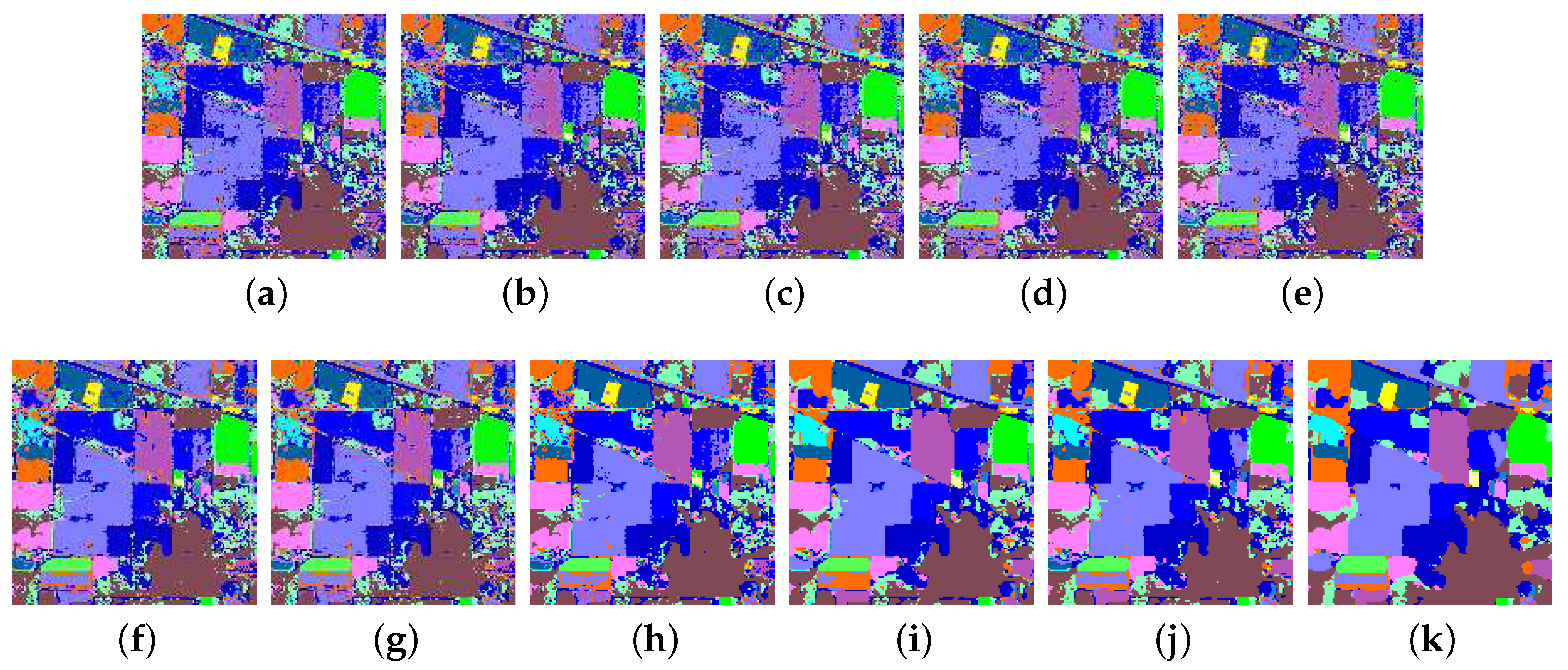
Figure 7.
Classification maps and overall classification accuracy levels (in parentheses) obtained for the AVIRIS Indian Pines dataset using different classification methods. (a) KSRC (81.50), (b) KCRC (79.52), (c) KNLS (81.94), (d) KFCLS-dist (81.91), (e) KFCLS-prob (81.49), (f) JRM-dist (85.54), (g) JRM-prob (86.27), (h) CJRM-dist (89.64), (i) CJRM-prob (92.42), (j) PRM (91.29), (k) CPRM (92.73).
Figure 8.
Classification maps and overall classification accuracy levels (in parentheses) obtained for the AVIRIS Kennedy Space Center dataset using different classification methods. (a) KSRC (89.86), (b) KCRC (88.99), (c) KNLS (89.90), (d) KFCLS-dist (89.97), (e) KFCLS-prob (90.17), (f) JRM-dist (90.59), (g) JRM-prob (90.57), (h) CJRM-dist (95.04), (i) CJRM-prob (95.63), (j) PRM (95.51), (k) CPRM (95.75).
Figure 9.
Classification maps and overall classification accuracy levels (in parentheses) obtained for the ROSIS University of Pavia dataset using different classification methods. (a) KSRC (83.44), (b) KCRC (82.74), (c) KNLS (84.40), (d) KFCLS-dist (84.43), (e) KFCLS-prob (84.19), (f) JRM-dist (90.96), (g) JRM-prob (91.29), (h) CJRM-dist (97.23), (i) CJRM-prob (97.71), (j) PRM (97.98), (k) CPRM (98.57).
Figure 10.
Classification maps and overall classification accuracy levels (in parentheses) obtained for the ROSIS Center of Pavia dataset using different classification methods. (a) KSRC (96.49), (b) KCRC (96.44), (c) KNLS (96.65), (d) KFCLS-dist (96.65), (e) KFCLS-prob (96.65), (f) JRM-dist (97.45), (g) JRM-prob (97.50), (h) CJRM-dist (98.82), (i) CJRM-prob (98.74), (j) PRM (98.84), (k) CPRM (98.93).
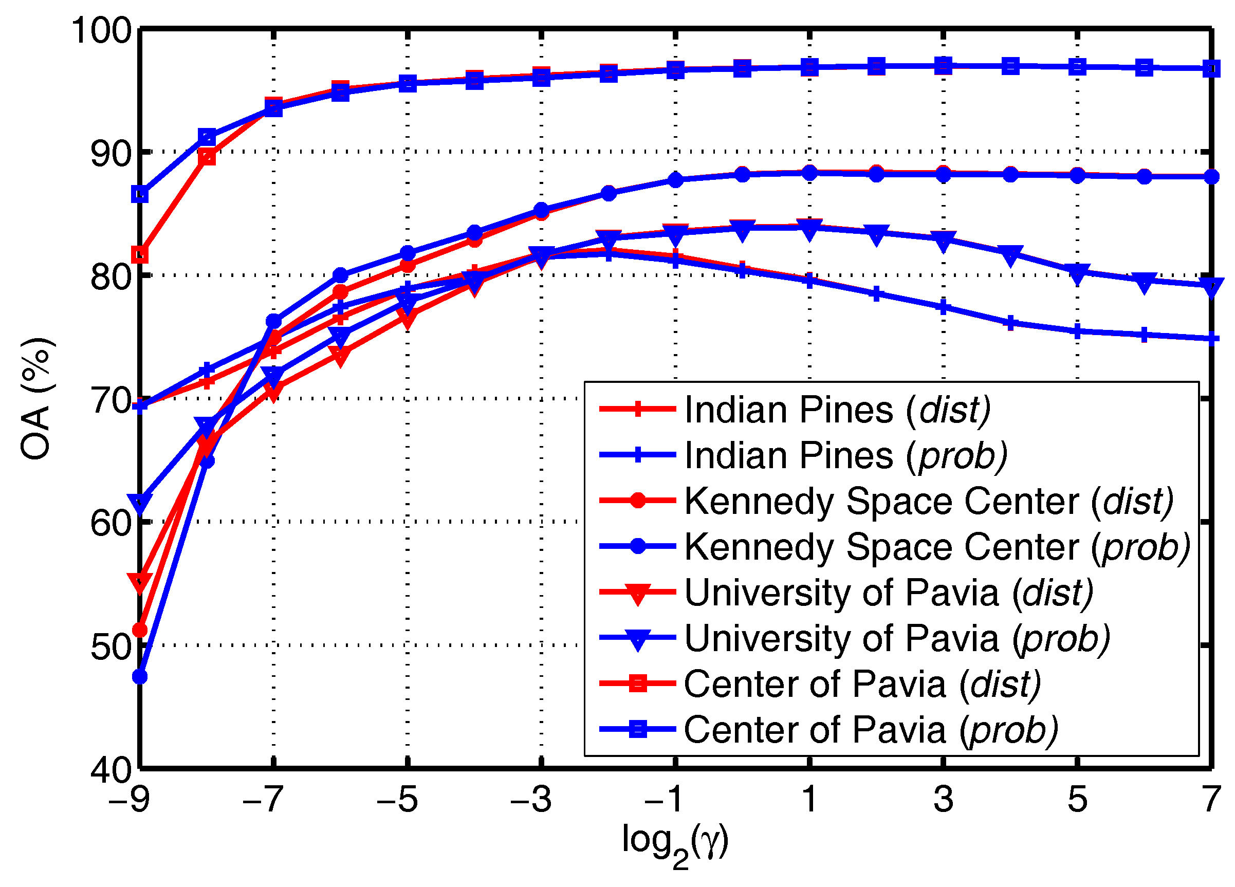
Figure 11.
OA as a function of for KFCLS when applied to the four given datasets.
Figure 11.
OA as a function of for KFCLS when applied to the four given datasets.
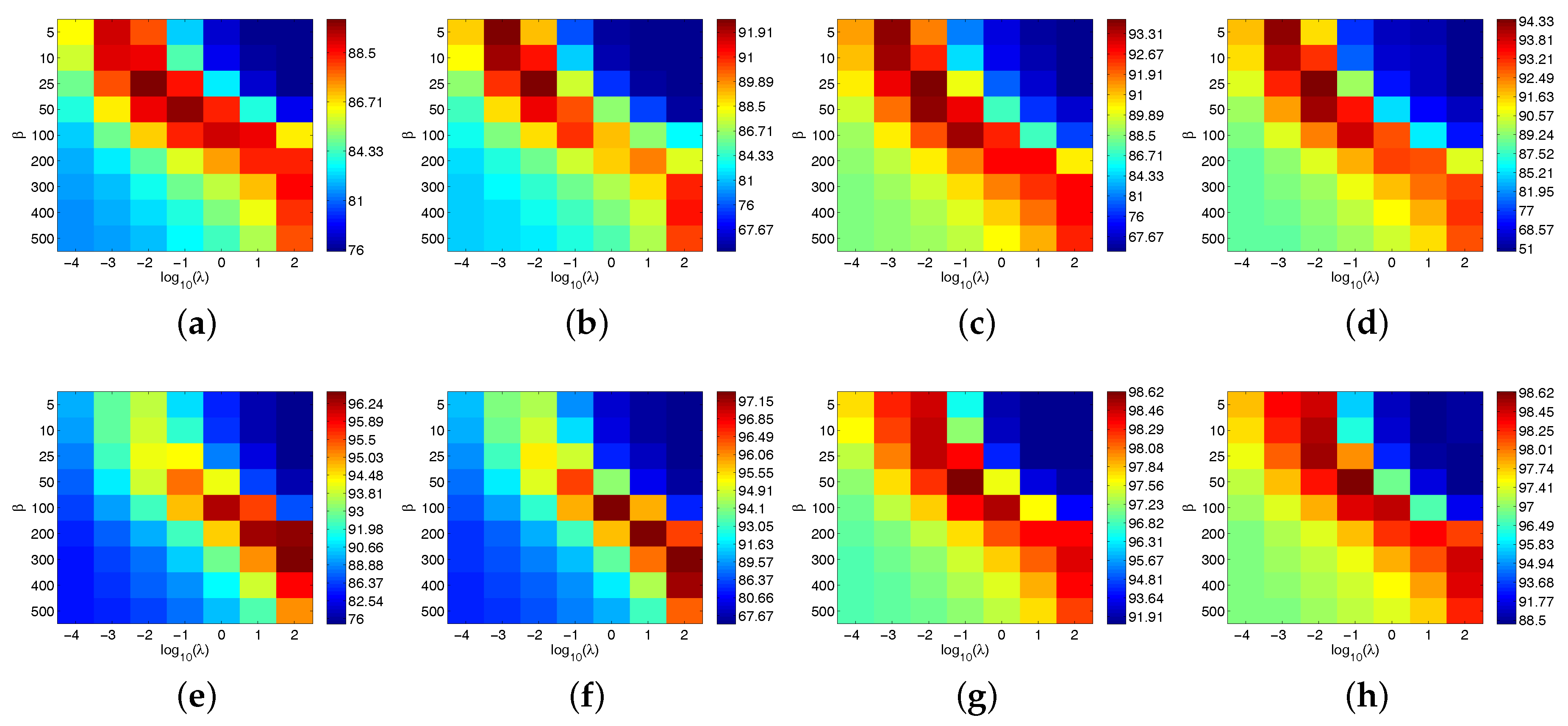
Figure 12.
OA with respect to and for CJRM when applied to the four given datasets. (a) CJRM-dist (Indian Pines), (b) CJRM-prob (Indian Pines), (c) CJRM-dist (Kennedy Space Center), (d) CJRM-prob (Kennedy Space Center), (e) CJRM-dist (University of Pavia), (f) CJRM-prob (University of Pavia), (g) CJRM-dist (Center of Pavia), (h) CJRM-prob (Center of Pavia).
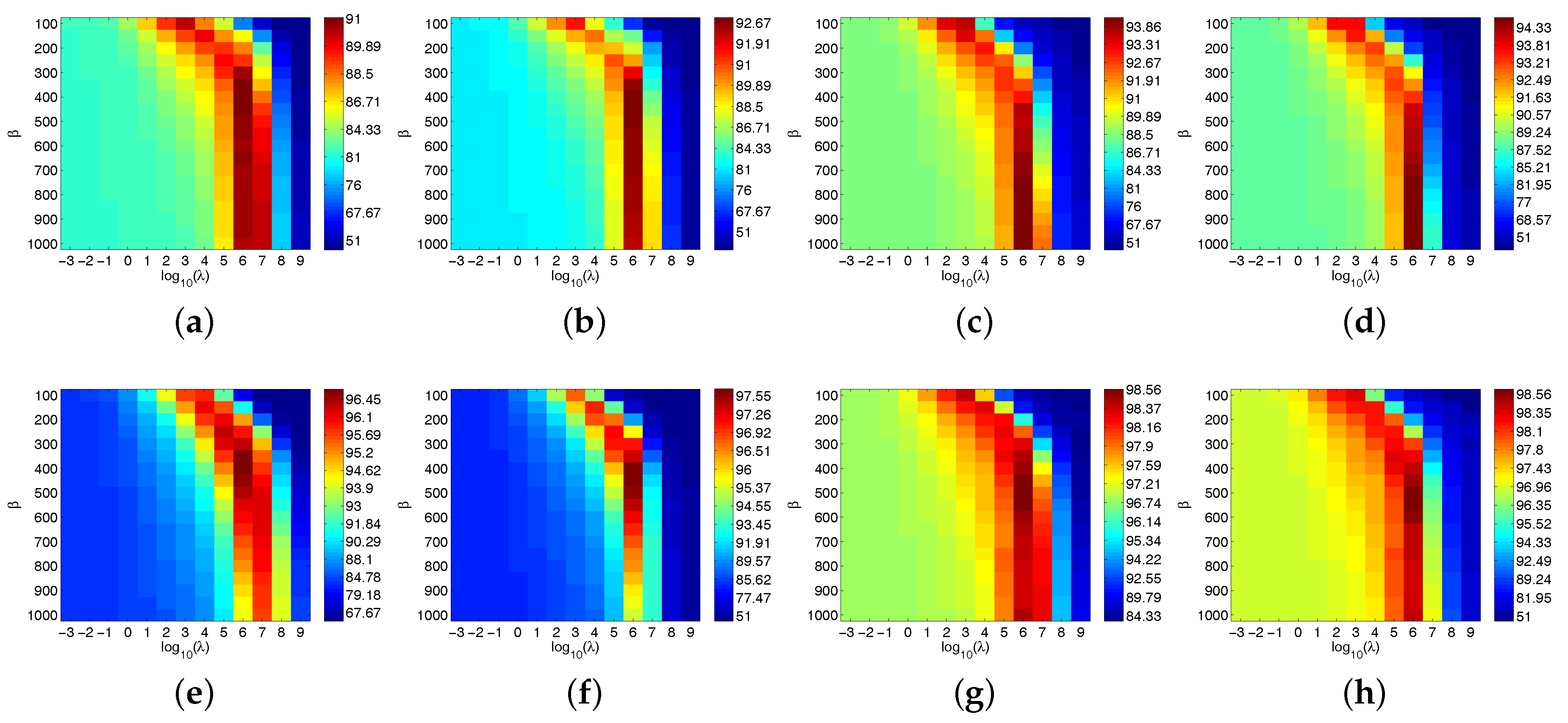
Figure 13.
OA with respect to and for PRM and CPRM when applied to the four given datasets. (a) PRM (Indian Pines), (b) CPRM (Indian Pines), (c) PRM (Kennedy Space Center), (d) CPRM (Kennedy Space Center), (e) PRM (University of Pavia), (f) CPRM (University of Pavia), (g) PRM (Center of Pavia), (h) CPRM (Center of Pavia).
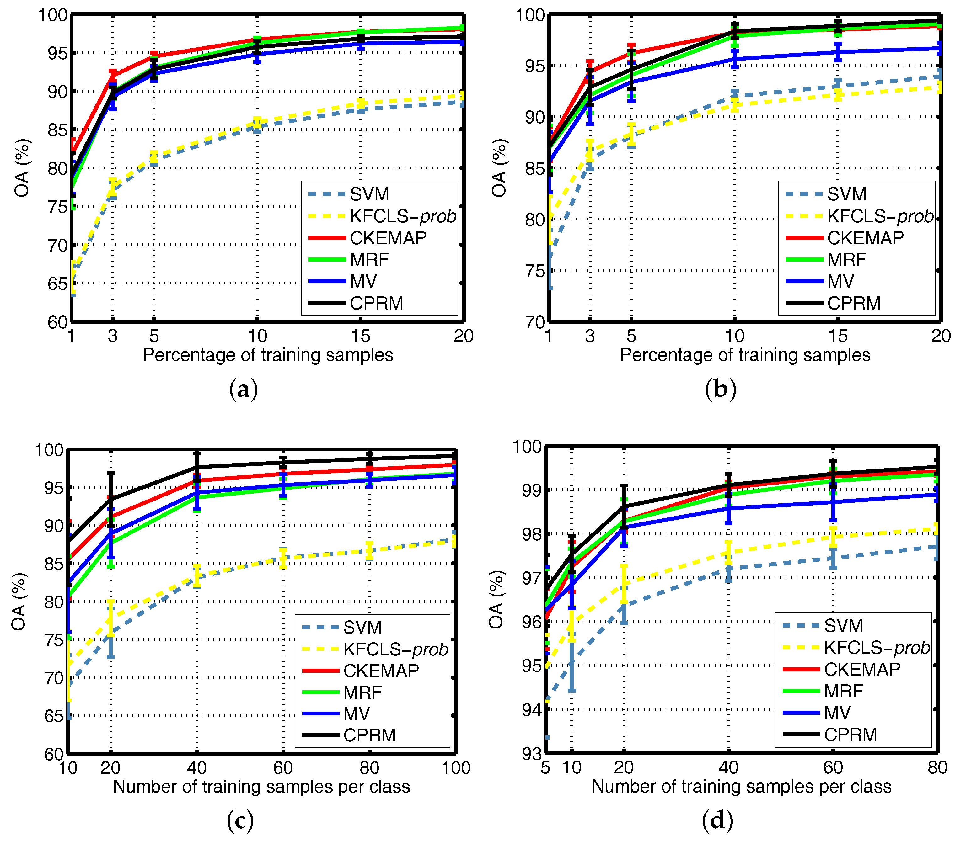
Figure 14.
OA as a function of the number of training pixels when applied to the four given datasets. (a) AVIRIS Indian Pines dataset, (b) AVIRIS Kennedy Space Center dataset, (c) ROSIS University of Pavia dataset, (d) ROSIS Center of Pavia dataset.
Figure 14.
OA as a function of the number of training pixels when applied to the four given datasets. (a) AVIRIS Indian Pines dataset, (b) AVIRIS Kennedy Space Center dataset, (c) ROSIS University of Pavia dataset, (d) ROSIS Center of Pavia dataset.
Table 1.
The ground reference classes in the AVIRIS Indian Pines dataset and the number of training and test pixels used in experiments.
Table 1.
The ground reference classes in the AVIRIS Indian Pines dataset and the number of training and test pixels used in experiments.
| No. | Class Name | Train | Test |
|---|
| C01 | Alfalfa | 3 | 51 |
| C02 | Corn-no till | 72 | 1362 |
| C03 | Corn-min till | 42 | 792 |
| C04 | Corn | 12 | 222 |
| C05 | Grass/pasture | 25 | 472 |
| C06 | Grass/trees | 38 | 709 |
| C07 | Grass/pasture-mowed | 2 | 24 |
| C08 | Hay-windrowed | 25 | 464 |
| C09 | Oats | 2 | 18 |
| C10 | Soybeans-no till | 49 | 919 |
| C11 | Soybeans-min till | 124 | 2344 |
| C12 | Soybean-clean till | 31 | 583 |
| C13 | Wheat | 11 | 201 |
| C14 | Woods | 65 | 1229 |
| C15 | Bldg-grass-tree drives | 19 | 361 |
| C16 | Stone-steel towers | 5 | 90 |
| Total | 525 | 9841 |
Table 2.
The ground reference classes in the AVIRIS Kennedy Space Center dataset and the number of training and test pixels used in experiments.
Table 2.
The ground reference classes in the AVIRIS Kennedy Space Center dataset and the number of training and test pixels used in experiments.
| No. | Class Name | Train | Test |
|---|
| C01 | Scrub | 39 | 722 |
| C02 | Willow swamp | 13 | 230 |
| C03 | Cabbage palm hammock | 13 | 243 |
| C04 | Cabbage palm/oak hammock | 13 | 239 |
| C05 | Slash pine | 9 | 152 |
| C06 | Oak/broadleaf hammock | 12 | 217 |
| C07 | Hardwood swamp | 6 | 99 |
| C08 | Graminoid marsh | 22 | 409 |
| C09 | Spartina marsh | 26 | 494 |
| C10 | Cattail marsh | 21 | 383 |
| C11 | Salt marsh | 21 | 398 |
| C12 | Mud flats | 26 | 477 |
| C13 | Water | 47 | 880 |
| Total | 268 | 4943 |
Table 3.
The ground reference classes in the ROSIS University of Pavia dataset and the number of training and test pixels used in experiments.
Table 3.
The ground reference classes in the ROSIS University of Pavia dataset and the number of training and test pixels used in experiments.
| No. | Class Name | Train | Test |
|---|
| C1 | Asphalt | 40 | 6812 |
| C2 | Meadow | 40 | 18,646 |
| C3 | Gravel | 40 | 2167 |
| C4 | Trees | 40 | 3396 |
| C5 | Metal sheets | 40 | 1338 |
| C6 | Bare soil | 40 | 5064 |
| C7 | Bitumen | 40 | 1316 |
| C8 | Bricks | 40 | 3838 |
| C9 | Shadows | 40 | 986 |
| Total | 360 | 43,563 |
Table 4.
The ground reference classes in the ROSIS Center of Pavia dataset and the number of training and test pixels used in experiments.
Table 4.
The ground reference classes in the ROSIS Center of Pavia dataset and the number of training and test pixels used in experiments.
| No. | Class Name | Train | Test |
|---|
| C1 | Water | 20 | 65,258 |
| C2 | Trees | 20 | 6488 |
| C3 | Meadow | 20 | 2885 |
| C4 | Bricks | 20 | 2132 |
| C5 | Soil | 20 | 6529 |
| C6 | Asphalt | 20 | 7565 |
| C7 | Bitumen | 20 | 7267 |
| C8 | Tile | 20 | 3102 |
| C9 | Shadows | 20 | 2145 |
| Total | 180 | 103,371 |
Table 5.
The optimal combination of parameters for the investigated methods when applied to the four given datasets. JRM: joint regularization model; CJRM: class-level JRM; KCRC: kernel collaborative representation classification; KFCLS: kernel fully constrained least squares; KNLS: kernel nonnegative constrained least squares; KSRC: kernel sparse representation classification; PRM: post-processing regularization model; CPRM: class-level PRM.
| | Pixel-Wise Classification | Spatial-Spectral Classification |
|---|
| | KSRC | KCRC | KNLS | KFCLS | JRM | CJRM | PRM | CPRM |
|---|
| | | – | | | | | | |
| Indian | | | | | | | | |
| Pines | | | – | – | | | | |
| | – | – | – | – | | | | |
| | | – | | | | | | |
| Kennedy | | | | | | | | |
| Space Center | | | – | – | | | | |
| | – | – | – | – | | | | |
| | | – | | | | | | |
| University | | | | | | | | |
| of Pavia | | | – | – | | | | |
| | – | – | – | – | | | | |
| | | – | | | | | | |
| Center | | | | | | | | |
| of Pavia | | | – | – | | | | |
| | – | – | – | – | | | | |
Table 6.
Classification accuracies for the two AVIRIS datasets using different classification methods. For both the pixel-wise classification and spatial-spectral classification, the best results are highlighted in bold, and the second best results are underlined. AA: average accuracy; KA: kappa coefficient of agreement; OA: overall accuracy.
| | Pixel-Wise Classification | Spatial-Spectral Classification |
|---|
| | KSRC | KCRC | KNLS | KFCLS | JRM | CJRM | PRM | CPRM |
|---|
| | dist | prob | dist | prob | dist | prob |
|---|
| Indian Pines |
| C01 | | 43.73 | 55.69 | 55.49 | | 58.24 | 59.61 | 60.59 | 65.88 | | |
| C02 | 78.35 | 73.28 | 78.55 | | | 83.37 | 84.05 | 84.06 | 83.66 | | |
| C03 | 64.31 | 53.03 | | 64.36 | | 71.19 | 72.85 | 79.39 | | 81.10 | |
| C04 | 52.12 | 41.40 | | 52.79 | | 56.98 | 60.18 | 68.06 | | 71.71 | |
| C05 | 89.03 | 86.17 | | | 88.98 | 89.85 | 90.04 | 90.74 | 91.61 | | |
| C06 | 96.46 | | 96.46 | | 95.85 | 97.24 | 97.08 | 98.28 | | 98.91 | |
| C07 | | 54.58 | 74.17 | | 70.42 | 88.33 | 87.92 | 87.08 | 88.33 | | |
| C08 | 98.75 | | 98.86 | | 98.47 | 99.18 | 99.09 | 99.38 | 99.44 | | |
| C09 | 57.78 | 36.11 | 57.78 | | | 67.78 | | 62.78 | | 59.44 | 36.67 |
| C10 | 72.87 | 61.60 | | 72.96 | | 77.60 | 79.34 | | | 87.66 | 88.07 |
| C11 | 82.42 | | 82.53 | | 82.43 | 88.70 | 88.38 | 92.76 | | 93.97 | |
| C12 | 76.76 | 65.04 | 78.16 | | | 85.51 | 88.64 | 92.26 | | 94.34 | |
| C13 | 98.76 | 98.86 | | | 98.51 | 99.00 | 99.05 | 99.25 | 99.30 | | |
| C14 | 95.28 | | | 95.66 | 95.29 | 97.27 | 97.05 | 98.13 | | 98.28 | |
| C15 | 53.80 | 41.94 | | 53.68 | | 52.96 | 56.37 | 62.88 | | 71.33 | |
| C16 | | 79.89 | | 87.33 | 68.78 | | 79.44 | | 80.89 | 86.22 | 85.00 |
| OA(%) | 81.34 | 78.99 | | | 81.46 | 85.53 | 86.15 | 89.49 | | 91.00 | |
| AA(%) | 77.28 | 69.93 | | | 76.42 | 81.23 | 82.20 | 84.40 | | 86.96 | |
| KA(%) | 78.66 | 75.69 | | | 78.80 | 83.44 | 84.17 | 88.00 | | 89.72 | |
| Time(s) | | | 15.89 | 19.50 | 19.19 | 47.26 | 46.95 | | | 20.08 | 19.28 |
| Kennedy Space Center |
| C01 | 95.69 | | 95.80 | | 95.79 | 97.58 | 97.62 | 99.47 | | 99.40 | |
| C02 | 85.09 | 85.04 | | | 84.87 | 85.74 | 85.78 | | | 89.96 | 91.09 |
| C03 | | | 90.08 | 90.08 | 90.29 | 97.16 | 97.20 | 98.11 | 98.19 | | |
| C04 | | 41.88 | 46.15 | 46.40 | | 50.92 | 50.63 | 52.80 | 54.60 | | |
| C05 | 61.64 | 59.14 | 61.64 | | | 70.66 | 70.99 | | | 79.87 | 80.53 |
| C06 | | 34.10 | 44.70 | 44.61 | | 36.27 | 36.36 | | | 61.80 | 61.38 |
| C07 | 83.54 | | 83.94 | 83.84 | | 90.10 | 90.40 | 97.58 | | 96.46 | |
| C08 | | 88.19 | 88.90 | 88.88 | | 93.81 | 93.94 | 97.87 | | 98.34 | |
| C09 | 96.01 | | | 96.30 | 96.28 | 97.96 | 97.96 | | 98.30 | | 98.30 |
| C10 | 95.30 | 94.15 | | | 93.24 | 96.66 | 96.58 | 98.64 | | 98.80 | |
| C11 | 94.30 | | 94.60 | 94.60 | | 95.38 | 95.15 | 97.09 | | 97.49 | |
| C12 | | 87.42 | 87.34 | 87.25 | | 87.25 | 87.48 | 92.01 | | 93.52 | |
| C13 | | | 99.69 | 99.72 | 99.34 | 99.89 | 99.90 | | | | |
| OA(%) | | 87.76 | 88.32 | | 88.29 | 89.97 | 90.00 | 93.56 | | 94.08 | |
| AA(%) | | 81.10 | 82.28 | 82.30 | | 84.57 | 84.61 | 90.04 | | 90.56 | |
| KA(%) | | 86.31 | 86.96 | | 86.94 | 88.80 | 88.83 | 92.81 | | 93.39 | |
| Time(s) | | | 117.8 | 142.0 | 140.3 | 965.5 | 963.1 | | | 156.1 | 155.3 |
Table 7.
Classification accuracies for the two ROSIS datasets using different classification methods. For both the pixel-wise classification and spatial-spectral classification, the best results are highlighted in bold, and the second best results are underlined.
Table 7.
Classification accuracies for the two ROSIS datasets using different classification methods. For both the pixel-wise classification and spatial-spectral classification, the best results are highlighted in bold, and the second best results are underlined.
| | Pixel-Wise Classification | Spatial-Spectral Classification |
|---|
| | KSRC | KCRC | KNLS | KFCLS | JRM | CJRM | PRM | CPRM |
|---|
| | dist | prob | dist | prob | dist | prob |
|---|
| University of Pavia |
| C1 | 73.25 | 72.78 | 74.77 | | | 80.03 | 80.29 | 94.73 | | 95.49 | |
| C2 | 83.24 | 82.61 | 83.55 | | | 87.70 | 88.32 | 96.64 | | 96.55 | |
| C3 | 78.68 | 77.64 | | | 78.52 | 84.72 | 84.63 | 86.77 | 87.08 | | |
| C4 | 91.65 | | | 92.61 | 91.23 | | 94.70 | 94.87 | 94.86 | | 93.37 |
| C5 | | 99.23 | 99.33 | | 98.27 | 99.24 | 98.67 | | 98.36 | 98.94 | |
| C6 | 84.77 | | | 85.48 | 84.72 | 93.04 | 93.17 | 98.78 | | 99.12 | |
| C7 | | | 92.54 | 92.36 | 92.29 | 96.75 | 96.78 | 99.59 | | 99.51 | |
| C8 | 77.99 | | | 78.57 | 78.37 | 87.93 | 87.82 | 95.88 | | | 96.14 |
| C9 | | 99.22 | 99.25 | | 98.80 | 99.29 | 98.92 | 99.37 | | 99.23 | |
| OA(%) | 82.96 | 83.05 | | | 83.39 | 88.45 | 88.71 | 96.13 | | 96.60 | |
| AA(%) | 86.77 | | | 87.20 | 86.79 | 91.52 | 91.48 | 96.21 | 96.75 | | |
| KA(%) | 78.21 | 78.37 | | | 78.72 | 85.16 | 85.47 | 94.94 | | 95.57 | |
| Time(s) | | | 101.7 | 119.1 | 117.2 | 344.1 | 342.1 | | | 124.5 | 119.0 |
| Center of Pavia |
| C1 | 99.67 | | 99.69 | 99.69 | | 99.86 | 99.90 | | | | |
| C2 | 91.09 | | 91.16 | | 91.07 | 91.71 | 91.67 | | | 95.86 | 96.62 |
| C3 | | | 89.60 | 89.59 | 89.25 | | 90.10 | 83.58 | 81.81 | | 88.72 |
| C4 | | 88.84 | 88.99 | | 88.72 | 90.85 | 90.78 | 99.38 | 99.09 | | |
| C5 | 87.95 | | 89.16 | 89.07 | | 93.21 | 93.39 | | | 95.54 | 96.23 |
| C6 | 96.84 | | 96.93 | 96.94 | | 97.95 | 98.01 | 99.55 | 99.50 | | |
| C7 | 86.29 | 85.52 | | | 86.23 | 88.78 | 88.64 | | | 93.25 | 93.44 |
| C8 | 98.83 | 98.76 | | | 98.83 | 99.22 | 99.15 | 96.94 | 96.66 | | |
| C9 | | 99.97 | 99.98 | | 99.97 | | | 95.96 | 95.20 | 94.04 | 93.69 |
| OA(%) | 96.74 | | 96.84 | 96.84 | | 97.56 | 97.56 | 98.56 | 98.52 | | |
| AA(%) | 93.31 | | | 93.44 | 93.40 | 94.72 | 94.63 | 96.01 | 95.73 | | |
| KA(%) | 94.40 | | 94.58 | 94.57 | | 95.80 | 95.80 | 97.52 | 97.45 | | |
| Time(s) | | | 91.89 | 109.3 | 106.9 | 462.3 | 460.6 | | | 116.8 | 110.7 |
Table 8.
OA as a function of the number of training pixels per class for different classification methods when applied to the two AVIRIS datasets. The standard deviation (in parentheses) of the ten random tests is also reported in each case. For both the pixel-wise classification and spatial-spectral classification, the best results are highlighted in bold, and the second-best results are underlined.
| | Pixel-Wise Classification | Spatial-Spectral Classification |
|---|
| | KSRC | KCRC | KNLS | KFCLS | JRM | CJRM | PRM | CPRM |
|---|
| | dist | prob | dist | prob | dist | prob |
|---|
| Indian Pines |
| 1% | | 66.12 | | 66.36 | 65.83 | 69.96 | 70.53 | 72.28 | 74.98 | | |
| (1.83) | (1.83) | (1.78) | (1.80) | (1.95) | (2.18) | (2.04) | (2.36) | (2.73) | (2.82) | (2.80) |
| 3% | 77.59 | 75.67 | | | 77.55 | 82.17 | 82.89 | 85.49 | | 87.49 | |
| (1.12) | (1.10) | (1.21) | (1.00) | (1.00) | (0.93) | (0.81) | (0.69) | (0.71) | (0.59) | (0.72) |
| 5% | 81.34 | 78.99 | | | 81.46 | 85.53 | 86.15 | 89.50 | | 91.00 | |
| (0.52) | (0.75) | (0.56) | (0.42) | (0.57) | (0.36) | (0.33) | (0.81) | (1.34) | (0.79) | (1.18) |
| 10% | 85.92 | 83.25 | | | 85.93 | 90.40 | 90.98 | 93.27 | 93.85 | | |
| (0.59) | (0.63) | (0.57) | (0.58) | (0.51) | (0.64) | (0.62) | (0.77) | (0.84) | (0.74) | (0.76) |
| 15% | 88.38 | 85.98 | | | 88.40 | 92.47 | 92.88 | 95.54 | | 95.98 | |
| (0.28) | (0.20) | (0.30) | (0.31) | (0.41) | (0.60) | (0.58) | (0.48) | (0.37) | (0.53) | (0.31) |
| 20% | 89.41 | 86.81 | | | 89.41 | 93.17 | 93.50 | 96.05 | | 96.29 | |
| (0.41) | (0.46) | (0.43) | (0.41) | (0.36) | (0.44) | (0.49) | (0.26) | (0.45) | (0.28) | (0.21) |
| Kennedy Space Center |
| 1% | | | 80.16 | 80.10 | 79.97 | 82.37 | 82.49 | 84.71 | 85.19 | | |
| (2.03) | (2.18) | (2.09) | (2.09) | (2.30) | (2.32) | (2.43) | (2.54) | (2.76) | (2.40) | (2.67) |
| 3% | 86.61 | 86.04 | | | 86.69 | 88.31 | 88.58 | 91.79 | 92.29 | | |
| (0.89) | (1.09) | (0.78) | (0.78) | (0.97) | (1.50) | (1.53) | (1.56) | (1.80) | (1.69) | (1.71) |
| 5% | | 87.76 | 88.32 | | 88.29 | 89.97 | 90.00 | 93.56 | | 94.08 | |
| (0.93) | (0.85) | (1.02) | (1.02) | (0.97) | (1.52) | (1.56) | (2.08) | (2.17) | (1.83) | (1.86) |
| 10% | 91.00 | 89.88 | 91.12 | | | 92.93 | 93.07 | 96.70 | 97.16 | | |
| (0.57) | (0.33) | (0.50) | (0.51) | (0.53) | (0.57) | (0.56) | (1.42) | (1.48) | (0.60) | (0.69) |
| 15% | 91.98 | 90.63 | | | 92.12 | 94.31 | 94.40 | 98.28 | | 98.49 | |
| (0.53) | (0.41) | (0.45) | (0.44) | (0.44) | (0.56) | (0.57) | (0.59) | (0.56) | (0.47) | (0.48) |
| 20% | 92.72 | 91.21 | | 92.84 | | 95.09 | 95.18 | 99.23 | | 99.18 | |
| (0.40) | (0.44) | (0.52) | (0.50) | (0.47) | (0.62) | (0.58) | (0.33) | (0.30) | (0.26) | (0.24) |
Table 9.
OA as a function of the number of training pixels per class for different classification methods when applied to the two ROSIS datasets. The standard deviation (in parentheses) of the ten random tests is also reported in each case. For both the pixel-wise classification and spatial-spectral classification, the best results are highlighted in bold, and the second-best results are underlined.
| | Pixel-Wise Classification | Spatial-Spectral Classification |
|---|
| | KSRC | KCRC | KNLS | KFCLS | JRM | CJRM | PRM | CPRM |
|---|
| | dist | prob | dist | prob | dist | prob |
|---|
| University of Pavia |
| 10 | 71.50 | 72.33 | | | 71.52 | 76.57 | 76.62 | 84.38 | | 85.59 | |
| (4.17) | (4.21) | (4.39) | (4.48) | (4.56) | (5.41) | (5.39) | (5.48) | (5.96) | (6.91) | (5.69) |
| 20 | 77.50 | 77.81 | | | 77.78 | 83.11 | 83.21 | 91.30 | | 91.97 | |
| (2.33) | (2.14) | (2.24) | (2.25) | (2.24) | (2.92) | (2.90) | (2.71) | (3.61) | (3.44) | (3.49) |
| 40 | 82.96 | 83.05 | | | 83.39 | 88.45 | 88.71 | 96.13 | | 96.60 | |
| (1.05) | (1.14) | (1.17) | (1.19) | (1.30) | (1.84) | (1.92) | (1.64) | (1.47) | (2.07) | (1.80) |
| 60 | 85.42 | 85.43 | | | 85.63 | 90.80 | 90.93 | 96.63 | | 97.16 | |
| (1.26) | (1.43) | (1.23) | (1.25) | (1.15) | (1.39) | (1.40) | (1.02) | (1.03) | (0.76) | (0.64) |
| 80 | 86.38 | 86.26 | | | 86.68 | 91.33 | 91.37 | 97.80 | | 98.17 | |
| (0.75) | (0.97) | (0.91) | (0.91) | (0.99) | (0.79) | (0.86) | (0.83) | (0.74) | (0.62) | (0.63) |
| 100 | 87.70 | 87.54 | | | 87.90 | 92.34 | 92.41 | 98.12 | 98.40 | | |
| (0.82) | (0.89) | (0.68) | (0.68) | (0.61) | (0.90) | (0.89) | (0.56) | (0.49) | (0.70) | (0.24) |
| Center of Pavia |
| 5 | 94.46 | 94.71 | | 94.79 | | 95.97 | 96.14 | 96.43 | | 96.60 | |
| (0.99) | (0.95) | (0.74) | (0.75) | (0.76) | (0.74) | (0.69) | (0.74) | (0.71) | (0.83) | (0.81) |
| 10 | 95.50 | | 95.89 | 95.88 | | 96.86 | 96.93 | 97.50 | 97.49 | | |
| (0.53) | (0.41) | (0.46) | (0.47) | (0.38) | (0.47) | (0.45) | (0.31) | (0.32) | (0.43) | (0.41) |
| 20 | 96.74 | | 96.84 | 96.84 | | 97.56 | 97.56 | 98.56 | 98.52 | | |
| (0.42) | (0.43) | (0.38) | (0.38) | (0.41) | (0.48) | (0.51) | (0.44) | (0.47) | (0.49) | (0.48) |
| 40 | 97.56 | 97.55 | | | 97.57 | 98.11 | 98.11 | 98.77 | 98.25 | | |
| (0.21) | (0.16) | (0.22) | (0.22) | (0.24) | (0.24) | (0.24) | (0.26) | (0.39) | (0.24) | (0.26) |
| 60 | 97.91 | 97.80 | | | 97.92 | 98.42 | 98.41 | 99.07 | 98.99 | | |
| (0.19) | (0.20) | (0.21) | (0.21) | (0.20) | (0.25) | (0.25) | (0.30) | (0.32) | (0.30) | (0.29) |
| 80 | 98.10 | 97.91 | | | 98.11 | 98.55 | 98.54 | 99.22 | 99.11 | | |
| (0.12) | (0.17) | (0.11) | (0.11) | (0.10) | (0.17) | (0.17) | (0.17) | (0.21) | (0.13) | (0.16) |


